Term Project Report for ME346 – INTRODUCTION TO MOLECULAR SIMULATIONS Instructor: Prof. Wei Cai Stanford University WAVE PROPOGATION IN SOLIDS USING MOLECULAR DYNAMICS SUBMITTED BY AMIRALI KIA ASHISH MITRA CHRIS WEINBERGER Stanford University

Table of Contents Abstract ............................................................................................................................... 3 Introduction......................................................................................................................... 3 Molecular Dynamics Simulation of Phonons ..................................................................... 5 Phonon Dispersion in Molybdenum ................................................................................... 7 Attenuation due to Vacancies ............................................................................................. 8 Nonlinear Vibrations......................................................................................................... 11 Conclusion ........................................................................................................................ 13 Appendix A Sample Script File for Simulation of Longitudinal Wave in a Crystal with Voids ........... 15 Appendix B Sample Script File for Simulation of Nonlinear wave in a Perfect Crystal...................... 17 References......................................................................................................................... 19

Abstract The authors have simulated plane waves in solids using molecular dynamics. The propagation of both transverse and longitudinal waves have been studied in three directions in a crystal and both small as well as large amplitudes have been taken into consideration. Attenuation of the waves due to the presence of a vacancy defect in the crystal was also studied. The simulation results did not show any visible effects on the attenuation of the waves, but on reducing the box size an interesting existence of a beat phenomenon was observed. The authors were successfully able to reproduce the analytical phonon dispersion curve for Mo using Molecular Dynamics simulation. From the nonlinear vibration analysis, the simulation results have shown that the wave splits into waves of a number of frequencies. Another interesting observation of large amplitude vibrations was that at maximum wave number the waves do not split and only a single frequency is seen to propagate. This effect is seen to be dominant until the crystal eventually melts. Introduction Wave propagation in solids is very important phenomenon from bridges to small crystals. In large structures such as bridges, waves have the ability to propagate through the structure and can cause large enough amplitudes to destroy them. Vibrations are important at the atomic scale as well, since very high frequency vibrations are responsible for thermal properties such as thermal conductivity. Just as light is a wave motion that is considered as composed of particles called photons, we can think of the normal modes of vibration in a solid as being particle-like. Quantum of lattice vibration is called a phonon. The easiest wave in a solid to imagine is a plane wave. In this case, a plane of material vibrates together in one direction while the wave passes through. The mathematical formula for a plane wave is u = u0 exp[ i (k x ± ω t) ] (1) where u is the displacement caused by the wave, u0 is the wave amplitude, k is the wave vector, x is the original particle position, t is time, and ω is the angular frequency. There are several models that can be used to predict how plane waves move through solids, the simplest being the continuum model. Continuum theory assumes that a material is continuous with infinitesimal spacing between the particles of the material. The propagation of a plane wave in 1D in solids according to continuum theory is given by [1]:

2

2

22

2 1tu

cxu

∂∂

=∂∂ (2)

3

The solution of this equation gives that the frequency with which a wave will propagate through the solid is directly proportional to the wave number. w = k c where w – frequency of propagation of the wave through the solid k – wave number of the wave c – speed of sound in the material The velocity of a wave through the solid is a constant as it depends on the material properties, namely the Young’s modulus and the density of the material. Hence, as it can be seem from the equation continuum theory predicts a linear relationship between frequency and wave number. In real crystals, there is a finite spacing that exists between the atoms which alters the wave number frequency relationship. One simple model, which can be found in Kittel [2] models atoms as masses connected to each other using springs as shown in the figure 1.

a

Figure 1. Simple Atom-Spring Model of Plane Wave Motion The equations of motion of the waves is given, from [2], as:

)2( 11 ssss uuuC

dtduM −+= −+ (3)

)sin( 214 KaM

C=ω (4) Thus as seen from the above equations, the equation of motion of the waves is a difference equation as opposed to a partial differential equation in the continuum case and its solution gives that the frequency is proportional to the absolute value of the sine of the wave number. Hence there is a nonlinear relationship between the frequency and the wave number. The relationship between the frequency and wave number is called phonon dispersion and their plot is known as the phonon dispersion curve. The phonon dispersion curve for this model as given by equation (4) above is shown in figure 2.

4

Figure 2. Phonon Dispersion Curve for Simple Atom Model

One important feature of the dispersion curve is the periodicity of the function. For unit cell length , the repeat period is , which is equal to the unit cell length in the reciprocal lattice. Therefore the useful information is contained in the waves with wave vectors lying between the limits

ak

aππ

<≤−

This range of wave vectors is called the first Brillouin zone. At the Brillouin zone boundaries the nearest atoms of the chain vibrate in the opposite directions and the wave becomes a standing wave. Also as shown in the curve the straight dotted line represents the dispersion curve as would be predicted by the continuum theory showing a linear relationship between frequency and wave number. The solid line represents the dispersion curve as would be predicted by the simple atomistic theory showing a nonlinear relationship between frequency and wave number towards the edges of the Brillouin zone.

Vibrations in real crystals are much more complicated than what is suggested above. Planes of atoms can vibrate and the waves can propagate in many directions. The direction the wave propagates combined with the spatial wavelength is called its wave vector, k, and the magnitude of the wave vector is the wave number, k. To make notation simpler, the actual wave number is not used but the ratio of the wave number to the wave number at the Brillouin zone. This ratio is referred to as the k-ratio, and is always referred to a crystallographic direction. The amplitude of vibration is also a vector,u0, denoting the direction of the vibration as well as its size.

Molecular Dynamics Simulation of Phonons In order to simulate waves in crystalline solids, first a wave must be introduced into the solid. The simplest wave is a plane wave, which can be represented as u = u0 exp[ i (k x ± ω t) ] (5)

5

This wave can further be simplified by reducing our consideration to one family of plane waves u = u0 cos(k x) cos(ω t) (6)

which is a standing wave. This wave can be thought of the superposition of two plane waves, each of equal amplitude, traveling in opposite directions. The usefulness of choosing a plane wave will become apparent later when measuring output is discussed.

Not every wave vector k can be introduced into a molecular dynamics simulation. Since most MD simulations utilize Periodic Boundary Conditions (PBC), this limits the number of wave vectors studied to be periodic in the box. If the simulation is carried out in a cubic material with equal repeat vectors in each direction of length L, the possible wave vectors that will produce a standing wave are k=2nπ/Lwhere n is an integer. Waves of shorter wavelengths will not represent a simple cosine wave form since the periodic boundary conditions will create imperfect images of the wave in the periodic boxes. The wave vector is specified as an input to an MD simulation; however its relationship to the frequency is unknown. Also, if attenuation of the wave does occur, the amplitude of the wave as a function of time is also unknown. One method of measuring wave frequency and amplitude ratio is by measuring kinetic energy of the simulation of a standing wave. The particle velocity of a wave is simply the derivative of (ref above)

)sin()cos( tdtd ωω kxuu

o−= (7)

The kinetic energy can thus be written as

)(sin)(cos21 2222

0 tuV

ωωρ∫ kx (8)

Carrying out this integration, and noting that the wave vector is periodic in the box

)(sin41 222

0 tuV ωωρ (9)

which can be re-written as

)]2sin(1[81 22

0 tuV ωωρ − (10)

Thus, the kinetic energy is sinusoidal in time with a frequency of twice the frequency of the waveform. The kinetic energy is also proportional to the square of the wave amplitude, enabling attenuation of the wave to be measured through a drop in kinetic energy amplitude.

6

Phonon Dispersion in Molybdenum Phonon Dispersion was studied in Crystal Molybdenum in Molecular Dynamics using the Finnis-Sinclair potential [6]. The simulations are performed using MD++ package [7]. The Mo crystal simulated was a perfect BCC structure repeated 12 times in each direction with periodic boundary conditions. A standing wave was introduced into the solid according to the description of the previous chapter, and the wave frequencies were recorded. All of the simulations were run for 1000 time steps, and the time step was varied according to the frequency, but ranged from 0.5 femto-seconds to 0.125 femto-seconds. The same simulation box was used for every simulation, only the wave vector and time steps were changed. Phonons in crystal Mo travel along the three crystallographic directions that contain planes of atoms. These three directions are the [100], [110], and [111] directions. Only waves that propagate in these three directions were studied.

0

1

2

3

4

5

6

7

8

9

10

0 6 12 18 24 30

K ratio

Freq

uenc

y TH

z

LongitudinalTransverseTransverse 1Transverse2

[100] [111] [110]

0.5 1.0 0.50.0 0.0 0.5

Figure 3. Phonon Dispersion Curve for Mo In the [100] direction, 12 waves were introduced into the solid for the longitudinal and transverse waves. The transverse waves have an amplitude direction of [010] and [001], and they are degenerate. These waves have wave numbers of k = n π / 12 a, where n is an integer from 1 to 12, and a is the lattice constant. The wave number π/a is the edge of the first Brillion zone in the [100] direction. Wave propagation in the [111] direction is very similar to the [100] direction. It has a Brillion zone boundary at π/a√3 and each phonon dispersion curve is simulated with 12 waves with the same wave numbers. The transverse waves are also degenerate, and the chosen amplitude directions are the [1-10] and [11-2] directions.

7

The [110] direction has its first Brillion zone boundary at π/a2√2, and thus only 6 simulations are used. The transverse waves are in the [1-10] and [001] directions, are not degenerate, and the two waveforms propagate with different frequencies. This suggests that a transverse wave in an arbitrary direction with a wave vector in the [110] direction must be a combination of the two waves simulated. The phonon dispersion curves that were simulated are shown together in figure 3 above. The phonon dispersion curve can be calculated analytically using the Finnis-Sinclair potential as shown in figure 4 by [3]. Figure 4 also shows experimental data from Simonelli [4].

0

1

2

3

4

5

6

7

8

9

10

Γ H P Γ N

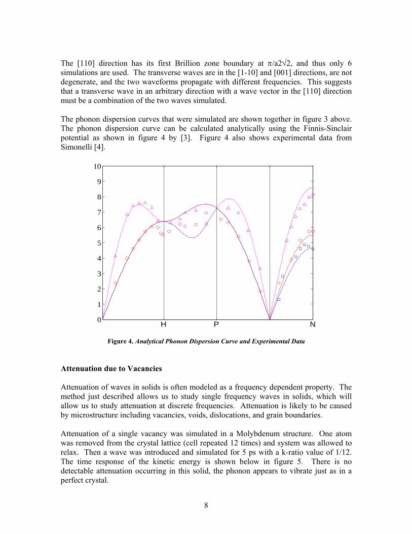
Figure 4. Analytical Phonon Dispersion Curve and Experimental Data Attenuation due to Vacancies Attenuation of waves in solids is often modeled as a frequency dependent property. The method just described allows us to study single frequency waves in solids, which will allow us to study attenuation at discrete frequencies. Attenuation is likely to be caused by microstructure including vacancies, voids, dislocations, and grain boundaries. Attenuation of a single vacancy was simulated in a Molybdenum structure. One atom was removed from the crystal lattice (cell repeated 12 times) and system was allowed to relax. Then a wave was introduced and simulated for 5 ps with a k-ratio value of 1/12. The time response of the kinetic energy is shown below in figure 5. There is no detectable attenuation occurring in this solid, the phonon appears to vibrate just as in a perfect crystal.

8

0 0.5 1 1.5 2 2.5 3 3.5 4 4.5 50

0.02

0.04

0.06

0.08

0.1

0.12

Time (ps)

Kinetic Energy (eV)

Figure 5. Kinetic Energy Plot for Vacancy with k-ratio=1/12

In order to obtain some results, the box size was reduced from 12 repeats to 5 in each direction. The k-ratio of the wave simulated is 1/5, the minimum in the new box. The time response of the kinetic energy is shown below for 5 picoseconds and 50 picoseconds in figures 6 and 7 below.

9

0 0.5 1 1.5 2 2.5 3 3.5 4 4.5 50

0.005

0.01

0.015

0.02

0.025

0.03

0.035

0.04

Time (ps)

Kinetic Energy (eV)

Figure 6. Kinetic Energy Plot for Vacancy and k-ratio 1/5

0 5 10 15 20 25 30 35 40 45 500

0.005

0.01

0.015

0.02

0.025

0.03

0.035

0.04

Time (ps)

Kinetic Energy (eV)

Figure 7. Kinetic Energy Plot of Beat Phenomenon

10

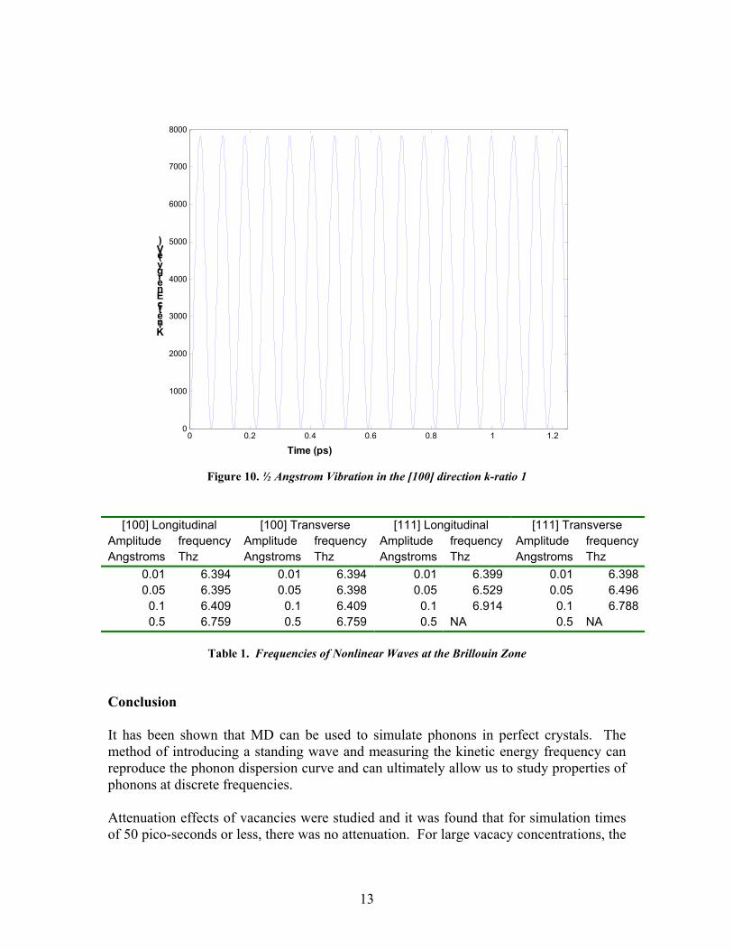
These figures illustrate that there is likely no attenuation occurring in the solid. The time pattern that does occur is called the beat phenomenon [5]. This occurs when the time signal is a sum of two sinusoids that are very near in frequency. Using a least squares best fit of this data, the frequencies of the two signals are 3.99 Thz and 4.06 Thz. The amplitudes of the two signals are not equal, the ratio of the former to the latter is approximately 0.6. The beat pattern may occur in simulation using a crystal repeat of 12, however the second waveform may have such a close frequency and small amplitude such that its effects are unnoticeable. This may suggest that as the vacancy concentration increases, the frequency difference of split waves increases and the amplitude ratio may move closer to unity. From this simulation we do not expect to see any attenuation due to vacancies. One reason attenuation might not occur in the simulation is that the simulated time may be too small. Nonlinear Vibrations Phonon vibrations are assumed to be very low amplitude vibrations of crystalline solids which allows the use of linear force-displacement relations which give rise to sinudoidal waves. If the atoms are displaced far enough the forces and displacements are not linearly related and the vibrations become nonlinear. An interesting point on the phonon dispersion curve is at the end of the Brillouin zone for the [100] and [111] directions. Here, the longitudinal and transverse waves of both directions converge to the same frequency. MD simulations of the nonlinearity show that the vibrations do not have a strong nonlinear behavior. MD simulations were carried out using the simulation box used to create the phonon dispersion curves. The wave vector was set to the maximum, and a time step of 0.125 fs was used. All the simulations were run for 1.25 ps. The results show that the waves at even very high amplitudes (0.5 angstrom) only exhibit single frequency oscillation. Figure 10 shows the time response of the kinetic energy for a longitudinal wave in the [100] direction with a 0.5 angstrom amplitude. All simulations at the Brillouin zone wave number in the [100] and [111] directions showed this type of response, though the frequencies did vary some. To contrast this, figure 8 shows the kinetic energy response of a 0.5 angstrom wave in the [111] direction for a wave number of 1, the minimum for the box size. Table 1 below shows the frequencies of the waves, both longitudinal and transverse, as a function of the wave amplitude for the [100] and [111] directions.

11

0 0.5 1 1.5 2 2.50

50

100

150

200

250

Time (ps)

Kinetic Energy (eV)

Figure 8. ½ Angstrom Vibration in the [111] direction k-ratio 1/12

0 0.2 0.4 0.6 0.8 1 1.20

0.5

1

1.5

2

2.5

3x 104

Time (ps)

Kinetic Energy (eV)

Figure 9. ½ Angstrom Vibration in the [111] direction k-ratio 1

12

0 0.2 0.4 0.6 0.8 1 1.20

1000

2000

3000

4000

5000

6000

7000

8000

Time (ps)

Kinetic Energy (eV)

Figure 10. ½ Angstrom Vibration in the [100] direction k-ratio 1

[100] Longitudinal [100] Transverse [111] Longitudinal [111] Transverse Amplitude frequency Amplitude frequency Amplitude frequency Amplitude frequencyAngstroms Thz Angstroms Thz Angstroms Thz Angstroms Thz

0.01 6.394 0.01 6.394 0.01 6.399 0.01 6.3980.05 6.395 0.05 6.398 0.05 6.529 0.05 6.496

0.1 6.409 0.1 6.409 0.1 6.914 0.1 6.7880.5 6.759 0.5 6.759 0.5 NA 0.5 NA

Table 1. Frequencies of Nonlinear Waves at the Brillouin Zone

Conclusion It has been shown that MD can be used to simulate phonons in perfect crystals. The method of introducing a standing wave and measuring the kinetic energy frequency can reproduce the phonon dispersion curve and can ultimately allow us to study properties of phonons at discrete frequencies. Attenuation effects of vacancies were studied and it was found that for simulation times of 50 pico-seconds or less, there was no attenuation. For large vacacy concentrations, the

13

kinetic energy split into two waves with nearly equal frequencies creating a beat phenomenon. Nonlinear crystal vibrations were also investigated at the end of the Brillion zone for [100] and [111] directions. At this point, it appears that even very high amplitude vibrations occur at single frequencies unlike nonlinear vibrations at lower wave number waves.

14

Appendix A – Sample Script File for Simulation of Longitudinal Wave in a Crystal with Voids # -*-shell-script-*- # mowave_long_voids.script # Chris Weinberger - Wei Cai # ME 346 - Molecular Simulations # # This script creates a perfect BCC Mo crystal # it creates a vacancy by removing 1 atom # relaxes the system using conjugate gradient relaxation # introduces a sinusoidal wave and saves Kinetic Energy # setnolog setoverwrite dirname = runs/mo-example shmsize = 31457280 shmallocate #10MB #-------------------------------------------- #Read in potential file # potfile = ~/Codes/MD++/potentials/mo_pot readpot #------------------------------------------------------------ #Create Perfect Lattice Configuration # latticestructure = body-centered-cubic latticeconst = 3.1472 #(A) for Mo makecnspec = [ 1 0 0 5 0 1 0 5 0 0 1 5 ] makecn finalcnfile = perf.cn writecn #------------------------------------------------------------ #Remove 1 atom # # Remove atoms - 1 In the corner (atom #0) pickfixedatomspec = [ 1 0 ] removepickedatoms # # #------------------------------------------------------------ # Relax after atom is removed # #Conjugate-Gradient relaxation conj_ftol = 1e-4 conj_itmax = 1000 conj_fevalmax = 1000 conj_fixbox = 1 #conj_monitor = 1 conj_summary = 1 relax finalcnfile = relaxed.cn writecn #sleep quit #quit #------------------------------------------------------------- #Initiate a wave form # # Wave Amplitude 0.01 Angstroms (Linear-small Amplitude) # Oscillation Direction [1 0 0] # Wave Vector [1 0 0] in reducec coordinates # # mkwavespec = [ 1 0.01 #wave amplitude in Angstrom

15

1 0 0 #osillation direction (will be normalized) 1 0 0 #wave vector in reduced space 0 #0: no velocity, 1: with velocity ] makewave #------------------------------------------------------------- #Plot Configuration atomradius = 1.0 bondradius = 0.3 bondlength = 0 atomcolor = cyan highlightcolor = purple backgroundcolor = gray bondcolor = red fixatomcolor = yellow energycolorbar = [ 1 -6.8 -6.55 ] highlightcolor = red plot_select = 3 plot_highlight = [ 0 0 1 2 3 4 5 6 7 8 9 ] plotfreq = 10 rotateangles = [ 0 0 0 1.1 ] # win_width = 600 win_height = 600 openwin alloccolors rotate saverot refreshnnlist eval plot #sleep quit #------------------------------------------------------------- #MD setting # scalevelocity = 0 equilsteps = 0 timestep = 0.0005 # (ps) atommass = 95.94 #Mo: Atomic Mass (g/mol) totalsteps = 100000 plotfreq = 50 #saveprop = 0 saveprop = 1 savepropfreq = 10 openpropfile run sleep quit

16

Appendix B – Sample Script File for Simulation of Nonlinear wave in a Perfect Crystal # -*-shell-script-*- # mowave_nonlinear.script # Chris Weinberger - Wei Cai # ME 346 - Molecular Simulations # # This script creates a perfect Mo Lattice # It introduces a sinusoidal wave into the solid # with a large amplitude and records Kintetic Energy # setnolog setoverwrite dirname = runs/mo-example shmsize = 31457280 shmallocate #10MB #-------------------------------------------- #Read in potential file # potfile = ~/Codes/MD++/potentials/mo_pot readpot #------------------------------------------------------------ #Create Perfect Lattice Configuration # latticestructure = body-centered-cubic latticeconst = 3.1472 #(A) for Mo makecnspec = [ 1 0 0 12 0 1 0 12 0 0 1 12 ] makecn finalcnfile = perf.cn writecn #------------------------------------------------------------ #Initiate a wave form # # Nonlinear (large Amplitud) Waveform # Oscillation Direction [1 1 1] # Wave Vector [12 12 12] # mkwavespec = [ 1 0.5 #wave amplitude in Angstrom 1 1 1 #osillation direction (will be normalized) 12 12 12 #wave vector in reduced space 0 #0: no velocity, 1: with velocity ] makewave #------------------------------------------------------------- #Plot Configuration atomradius = 1.0 bondradius = 0.3 bondlength = 0 atomcolor = cyan highlightcolor = purple backgroundcolor = gray bondcolor = red fixatomcolor = yellow energycolorbar = [ 1 -6.8 -6.55 ] highlightcolor = red plot_select = 3 plot_highlight = [ 0 0 1 2 3 4 5 6 7 8 9 ] plotfreq = 10 rotateangles = [ 0 0 0 1.1 ] # win_width = 600 win_height = 600 openwin alloccolors rotate saverot refreshnnlist eval plot #sleep quit #-------------------------------------------------------------

17

#Conjugate-Gradient relaxation conj_ftol = 1e-7 conj_itmax = 1000 conj_fevalmax = 1000 conj_fixbox = 1 #conj_monitor = 1 conj_summary = 1 #sleep quit #quit #------------------------------------------------------------- #MD setting scalevelocity = 0 equilsteps = 0 timestep = 0.00025 # (ps) atommass = 95.94 #Mo: Atomic Mass (g/mol) totalsteps = 10000 plotfreq = 50 #saveprop = 0 saveprop = 1 savepropfreq = 10 openpropfile run sleep quit

18

References

[1] L. Kinsler et al, Fundamentals of Acoustics 4th ed. (Wiley, New York, 1999). [2] C. Kittel, Introduction to Solid State Physics 7th ed. (Wiley, New York, 1995). [3] W. Cai, Unpublished. [4] G. Simonelli, R. Pasianot, and E. J. Savino, Phys. Rev. B 55, 5570 (1997). [5] L. Meirovitch, Elements of vibration analysis 2nd ed. (McGraw-Hill, New

York,1986). [6] M.W. Finnis and J.E. Sinclair, Philos. Mag. A 50, 45 (1984). [7] MD++ Simulation Package, Wei Cai, http://micro.stanford.edu/~caiwei/MD++

19