Embed Size (px)
Citation preview

Modern Reliability and
Maintenance Engineering
for Modern Industry
Piero Baraldi, Francesco Di Maio, Enrico Zio
Politecnico di Milano, Department of Energy, Italy
ARAMIS Srl, Italy

Research & Innovation consulting approach
History
MissionApproach
Main Intervention Areas
RESEARCH INNOVATION MARKET DELIVERY
HIG
HL
OW
IndustryUniversity
PO
SIT
ION
ING
ARAMIS & LASAR : the identity card
Large amount of deployed algorithms
(more than 20yrs R&D)
Advanced Reliability Availability & Maintenance for Industries and Services
Simulation, Modeling, Analysis, Research
for Treasuring Knowledge, Information and Data
SM
AR
T K
ID
Data
Information
Knowledge

The Team
ARAMIS Members (7):
Enrico Zio (President)
Michele Compare (Partner, CEO)
Piero Baraldi (Partner) Francesco Di Maio (Partner) Giovanni Sansavini (Partner)
Francesco Cannarile (Research consultant) Rodrigo Mena (Research consultant)
+ Network of senior experts on specifictechnical areas
LASAR Members (3):
Piero Baraldi (Associate Professor, PhD)
Francesco Di Maio (Assistant Professor, PhD)
Enrico Zio (Full Professor, PhD)
LASAR Post-Docs (3):
Michele Compare (PhD)
Rodrigo Mena (PhD)
Sameer Al Dahidi (PhD)
LASAR PhD students (7):
Marco Rigamonti
Francesco Cannarile
Wei Wang
Zhe Yang
Shiyu Chen
Alessandro Mancuso
Edoardo Tosoni
+ MSc students (10-12/y)
+ Visiting (4-6/y)

Industry 1-2-3-4

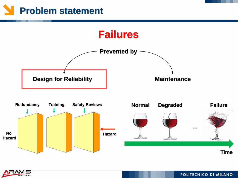
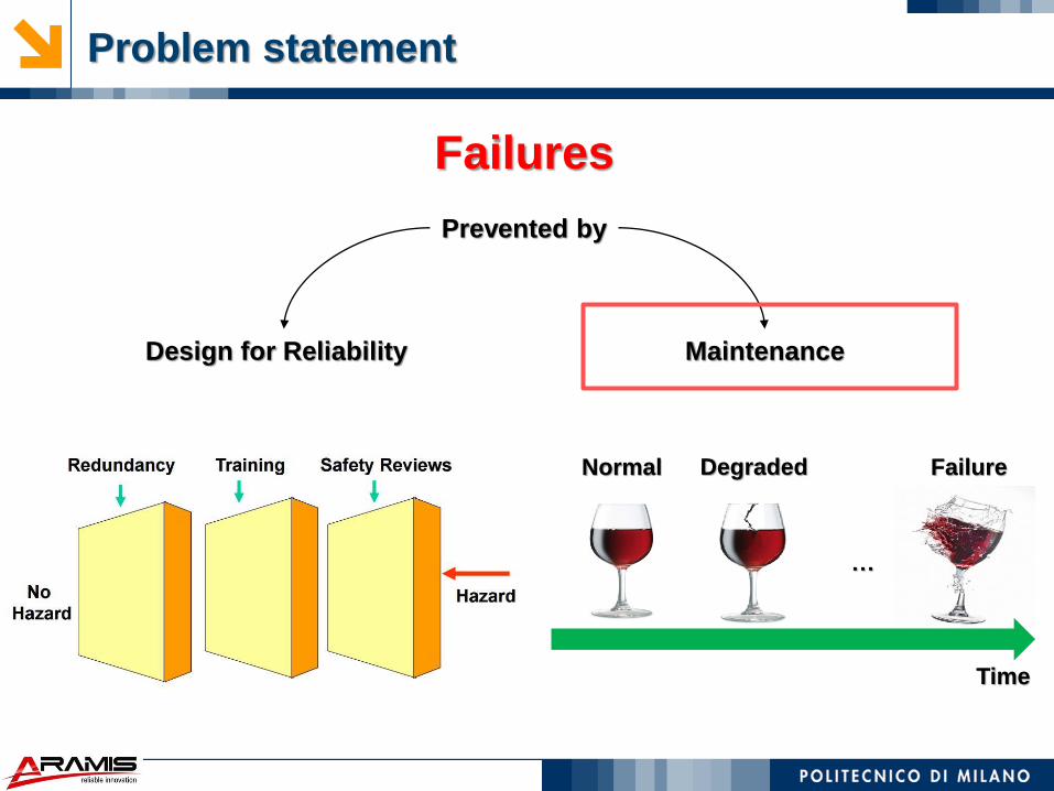
Prevented by
Design for Reliability Maintenance
Time
Normal Degraded Failure
Problem statement
Failures
…

(SMART) Reliability Engineering
Modern Reliability Engineering

The Big KID
Modern (smart) Reliability Engineering

Big Knowledge(ID)
Mathematical
problem
Real world
problem
Mathematical
solution
Real world
solution
formulation
interpretation

Big (K)Information(D)

Big (KI)Data
11101010010100010111001001010110000101010011101110111011101010010100010111001001010110000101010011101110111011101010010100010111001001010110000101010011101110111011101010010100010111001001010110000101110101001010001011100100101011000010101001110111011101110101001010001011100100101011000010101001110111011101110101001010001011100100101011000010

Can the Big KID become SMART for
Reliability Engineering ?
Prevented by
Design for Reliability Maintenance
Time
Normal Degraded Failure
Problem statement
Failures
…
SMART Reliability Engineering
Big KID opportunities
Reliability analysis for Design for Reliability:
From (binary) failure modeling to degradation-to-failure modeling

Failure modelling (binary)
ON OFF
Failure
As Good As New Failed
t
X(t)
100%
0%
System unavailability U(t) = Pr[X (t) <100%]
U(t) = Pr[X (t) =0%]

OFF
Failure
Degradation
state 1
Degradation
state n1
Failure Mode 1
…
Degradation
state 1
Degradation
state nM
Failure Mode M
…
…ON
Multi-state:
t
100%
75%
50%
25%
0%
X(t)
D(t)Demand of system performance
System unavailability U(D,t) = Pr[X (t) < D(t)]
Degradation-to-failure modeling

How to represent and model the item behavior?
OFF
Failure
Degradation
state 1
Degradation
state n1
Failure Mode 1
…
Degradation
state 1
Degradation
state nM
Failure Mode M
…
…ON
Degradation-to-failure modeling
Multi-state:
Integrating physics-of-failure knowledge in reliability models Multi-State Physic-Based Models

ModelKID(Knowledge, Information, Data)
0 20 40 60 800.994
0.995
0.996
0.997
0.998
0.999
1
Year
Reliability
Sufficient failure
data
Physics knowledge
Expert judgment
Field data
Highly reliable
Statistical models
of time to failure
Stochastic process
models
Physics-based
models
Multi-state
models
Reliability ?
SMART Reliability Engineering
Challenges
Alloy 82/182 dissimilar metal weld of piping in a PWR primary coolant system

Multi-state physics model of crack development
in Alloy 82/182 dissimilar metal weld
Alloy 82/182 dissimilar metal weld of piping in a PWR primary coolant system
Physical laws
SMART Reliability Engineering
Multi-State Physic-Based Models

SMART Reliability Engineering
Opportunities
Degradation
process
Random
shock process
1) Random shocks
Valve Internal leak
Pump Failure state
3 2 1 0λ32 λ21 λ10
Pump Initial state
2) Dependences in degradation processes

20SMART Reliability Engineering
Opportunities
3) Maintenance
Preventive maintenance (a)
Corrective maintenance (b)Degradation
process
a
b
Uncertain parameters in degradation models
4) Uncertainty
Valve Internal leak
Pump Failure state
3 2 1 0λ32 λ21 λ10
Pump Initial state

Valve Internal leak
Pump Failure state
3 2 1 0λ32 λ21 λ10
Pump Initial state
21SMART Reliability Engineering
Challenges
Piecewise-deterministic Markov
process (PDMP)
Monte Carlo (MC) simulation
Finite-volume integration schemes
Prevented by
Design for Reliability Maintenance
Time
Normal Degraded Failure
Problem statement
Failures
…

Maintenance Engineering Objectives
• Optimization of the maintenance of production assets:
Maximize reliability (R)
Maximize production availability (A)
Minimize personnel, material, inventory costs
Maximize efficiency/effectiveness of maintenance interventions (M)
Trade-off internal/external maintenance efforts (M)
Fulfill safety/regulatory constraints (S)
Fulfill budgetary constraints (C)
…
In other words…
RAMS(+C)
for
BETTER PERFORMANCES WITH LOWER COSTS

How to achieve the objectives
Integrated maintenance process, supported and informed by knowledge of
components/systems/process behaviors through
high-quality data, real-time information
effective models and methods to process the information
effective organizational processes to implement the solutions
KID + Intelligence

SMART Maintenance Engineering
Big KID opportunities
Maintenance:
Integrating physics knowledge and data:
• Prognostics and Health Management (PHM)

Maintenance Intervention Approaches
Maintenance Intervention
Unplanned
Corrective
Replacement or
repair of failed units
Planned
Scheduled
Perform
inspections,
and possibly
repairs,
following a
predefined
schedule
Condition-based
Monitor the health
of the system and
then decide on
repair actions
based on the
degradation level
assessed
Predictive
Predict the
Remaining Useful
Life (RUL) of the
system and then
decide on repair
actions based on
the predicted RUL
PHM
Modelling is in support to proper maintenance planning and

Prognostics and Health
Management (PHM)
1950 1980 2000Corrective
Maintenance
Planned Periodic
Maintenance
Condition Based
Maintenance (CBM)
2016Predictive
Maintenance (PrM)
PHM is fostered by advancements in:
Maintenance
Sensor Algorithm Computation power
Maintenance

PHM for what?
PHM in support to CBM and PrM
28
EquipmentMaintenance
Decision
Abnormal
Conditions
Normal
Conditions
Anomaly of Type 1
Anomaly of Type 2
Anomaly of Type 3
Maintenance
No
Maintenance
Decision
Maker
Remaining Useful
Life (RUL)
Fault
Detection
Fault
Diagnostics
Fault
Prognostics
…
Vibration
t
Sensors
measurements
t
Temperature

Increase maintainability, availability, safety, operating
performance and productivity
Reduce downtime, number and severity of failure and
life-time cost
PHM: why? (Industry)

Improve cash flow, profit stream and utilization of assets
Guarantee long term business
Increase market share
PHM: why? (Business)

MODEL OF
EQUIPMENT
BEHAVIOR
IN NORMAL
CONDITION
1x
2x
rx
t
t
t
…
1x
2x
rx
t
t
t
…
Measured Signals
NORMAL OPERATION
MEASUREMENTS = RECONSTRUCTIONS
Signal
Reconstructions
Feedwater Pump
PHM: how? (Fault detection)

MODEL OF
EQUIPMENT
BEHAVIOR
IN NORMAL
CONDITION
1x
2x
rx
t
t
t
…
1x
2x
rx
t
t
t
…
Measured Signals
Signal
ReconstructionsFeedwater Pump
ANOMALOUS OPERATION
MEASUREMENTS ≠ RECONSTRUCTIONS
PHM: how? (Fault detection)
P. Baraldi, F. Di Maio, L. Pappaglione, E. Zio, R. Seraoui, “Condition Monitoring of Electrical Power Plant Components During Operational
Transients”, Proceedings of the Institution of Mechanical Engineers, Part O, Journal of Risk and Reliability, 226(6) 568–583, 2012.
Baraldi, P., Canesi, R., Zio, E., Seraoui, R., Chevalier, R. Genetic algorithm-based wrapper approach for grouping condition monitoring signals of
nuclear power plant components (2011) Integrated Computer-Aided Engineering, 18 (3), pp. 221-234.

• Signal measurements representative of the fault classes: «c1,c2,…cn, class»
PHM: how? (Fault diagnostics)
CLASSIFIER
Measured Signals Fault Types
(classes)
BWR feedwater system
(Swedish Forsmark-3)
c1c2…cn
Baraldi, P., Razavi-Far, R., Zio, E., “Classifier-ensemble incremental-learning procedure for nuclear transient identification at different operational
conditions”, (2011) Reliability Engineering and System Safety, 96 (4), pp. 480-488.
F. Di Maio, J. Hu, P. Tse, K. Tsui, E. Zio, M. Pecht, “Ensemble-approaches for clustering health status of oil sand pumps”, Expert Systems with
Applications, Volume 39, pp. 4847–4859, doi: 10.1016/j.eswa.2011.10.008

Data-
Driven
Model
Based
• Physics-based model of
the degradation process
• Measurement equation
• Current degradation trajectory
• A threshold of failure
• External/operational conditions
Degrading componentSimilar components
Particle filter
Monte Carlo
Simulation
• Degradation trajectories of similar
components
• Life durations of a set of similar
components
Hidden Semi-Markov
Models
Artificial Neural
Networks
Autoregressive (AR)
models
Similarity-based
methods
Neuro-fuzzy
systems
PHM: how? (Fault prognostics)
Kalman Filter

Health
Index
tp
tp
FAILURE THRESHOLD
Prognostic
model
tf
LUR ˆ
Health index
prediction
t
t
t
t
Rotating
machinery (e.g.
pump)
Baraldi, P., Cadini, F., Mangili, F., Zio, E. Model-based and data-driven prognostics under different available information (2013) Probabilistic
Engineering Mechanics, 32, pp. 66-79.
E. Zio, F. Di Maio, “A Data-Driven Fuzzy Approach for Predicting the Remaining Useful Life in Dynamic Failure Scenarios of a Nuclear Power Plant”,
Reliability Engineering and System Safety, RESS, 10.1016/j.ress.2009.08.001, 2009.
F. Di Maio, K.L. Tsui, E. Zio, “Combining Relevance Vector Machines and Exponential Regression for Bearing RUL estimation”, Mechanical Systems
and Signal Processing, Mechanical Systems and Signal Processing, 31, 405–427, 2012.
PHM: how? (Fault prognostics)

PHM: performance ?
• Accuracy

• Accuracy
Fault Detection:
Low rate of False Alarms
Low rate of Missing Alarms
False Alarm
Rates
Missing
Alarm
Rates
0.54% 0.98%
Detection
Model
Normal
Condition
PHM: performance ? (detection)
1x
2x
rx

• Accuracy
Fault diagnostics:
Low Misclassification rate
C1
C2
C3
Diagnostic
Model
Signals
o = true
= diagnostic model
Misclassification rate = 2.58%
PHM: performance ? (diagnostics)

• Accuracy
Prognostics
PHM: performance ? (prognostics)
100 200 300 400 500 600 7000
100
200
300
400
500
600
700
800
900
KF
Single Model
True RUL
time
[Days]
Predicted RUL
RU
L(t
)
Prognostic
model

FAULT DETECTION
4
0

Application: NPP feedwater pumps
• Reactor Coolant Pumps of a PWR NPP
• [
x4
P. Baraldi, R. Canesi, E. Zio, R. Seraoui, R. Chevalier, "Generic algorithm-based wrapper
approach for grouping condition monitoring signal of nuclear power plant components“.
Integrated Computer-Aided Engineering, Vol. 18 (3), pp. 221-234, 2011

MODEL OF
EQUIPMENT
BEHAVIOR
IN NORMAL
CONDITION
1x
2x
rx
t
t
t
…
1x
2x
rx
t
t
t
…
Measured Signals
Signal
ReconstructionsFeedwater Pump
ANOMALOUS OPERATION
MEASUREMENTS ≠ RECONSTRUCTIONS
PHM: how? (Fault detection)

The Auto-Associative Kernel Regression
(AAKR)
Empirical modeling refers to any kind of (computer) approximated
modeling based on empirical observations rather than on mathematically
describable relationships of the system modeled
1. Collect data measurements representative of the system behavior
2. Develop the empirical model using as training set the collected data
measurements
test measurements
reconstruction
measurements
test measurements

Available information
• Historical measurements of 94 stationary signals during 1 year of
operation
• EDF experts have considered 48 of the 94 measured signals as the
most important for the component condition monitoring

Signal Grouping
COMPARISON
AUTO-ASSOCIATIVE
MODEL OF PLANT BEHAVIOR IN
NORMAL CONDITION
MODEL 1
MODEL 2
MODEL m
MEASURED
SIGNALS
…
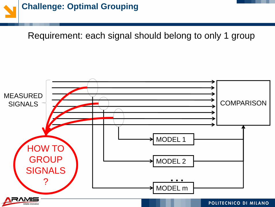
Challenge: Optimal Grouping
COMPARISON
MODEL 1
MODEL 2
HOW TO
GROUP
SIGNALS
?
MEASURED
SIGNALS
MODEL m
…
Requirement: each signal should belong to only 1 group

Approaches to signal grouping
HOW TO SPLIT THE SIGNALS INTO SUBGROUPS?
A-PRIORI CRITERIA
(signals divided on the basis of…)
• physical homogeneity
• location in the power plant
• correlation
• others
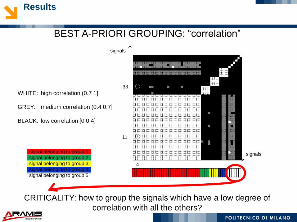
BEST A-PRIORI GROUPING: “correlation”
CRITICALITY: how to group the signals which have a low degree of
correlation with all the others?
Results
WHITE: high correlation (0.7 1]
GREY: medium correlation (0.4 0.7]
BLACK: low correlation [0 0.4]
4
11
33
signals
signalssignal belonging to group 1
signal belonging to group 2
signal belonging to group 3
signal belonging to group 4
signal belonging to group 5

Approaches to Signal Grouping
WRAPPER APPROACH
n SIGNALS
SEARCH
ENGINE
CANDIDATE
GROUPS
PERFORMANCE
EVALUATION
OPTIMAL
GROUPING
SEARCH ALGORITHM
HOW TO SPLIT THE SIGNALS INTO SUBGROUPS?
AAKR
A-PRIORI CRITERIA
(signals divided on the basis of…)
• location in the power plant
• correlation
• physical homogeneity
• others

The Wrapper Approach: Genetic Algorithms
SEARCH ENGINE
Genetic Algorithms
CHROMOSOME
n genes = n signals
PERFORMANCE EVALUATION
fitness = Accuracy
GENEsignal
1signal
2signal
3…
signali
… signal n
GROUP LABEL
(integer number)1 1 2 3 3 2 3

Results
OBTAINED GROUPINGS
correlation
GA
MAIN DIFFERENCE:
signals which have a low degree of correlation are divided in groups and/or
mixed with signals with a high degree of correlation

Results: Wrapper Approach
COMPARISON
DECISION
ŝ1
t
t
s1 – ŝ1
t
s1
ABNORMAL CONDITION:
seal deterioration
(SEAL
OUTCOMING
FLOW)
MEASURED SIGNALS
NORMAL
CONDITION
ABNORMAL
CONDITION
AUTO-ASSOCIATIVE
MODEL OF PLANT
BEHAVIOR IN NORMAL
CONDITIONS

FAULT CLASSIFICATION

0 500 1000 1500 2000 2500 3000 3500 4000 45000
500
1000
1500
2000
2500
Time
Sig
nal
Val
ue
Application: NPP turbine
AVAILABLE DATA:
• Number of transients: N=115
• Transient time length: 4500t
• Number of vibration signals: K=7

• examples are unlabeled
Scope
Find hidden
structure in data
Objective: Unsupervised Clustering for Fault Diagnosis
Feature 1
Fea
ture
2
The problem

Objective: Unsupervised Clustering for Fault Diagnosis
• examples are unlabeled
• there is no error or reward to
evaluate a potential solution
unsupervised
clustering
Feature 1
Fea
ture
2
2
3
1
v3
v2
v1
The problem

Methodology
STEP 1: feature extraction
STEP 2: unsupervised clusteringtime
Signal 1
Signal 2
Feature 1
Fea
ture
2
Feature 1
Fea
ture
2
Feature 1
Fea
ture
2 Fault class 2
v3
v2
v1
Fault class 3
Fault class 1

Feature Extraction: Fuzzy Similarity Analysis (1-D)
1- Transients pointwise difference computation:
i-th transient
2- Transients pointwise similarity computation:
μ (i,j) is the membership value of the distance δ(i,j) to the condition of “approximately zero”
3- Similarity Matrix W definition:
x(t)
Time (t)j-th transient
2
, 1,2,..., 1,2,...,T
i j
t i
i j x t x t i N j N
1 1, 2 ... 1,
2,1 1 2,3 ...
... 3, 2 ... 1,
,1 ... , 1 1
N
N N
N N N
N columns
N rows
Similarity between transients 2 and 3
j-th transient
i-th transient
5
8

Feature Extraction: Spectral Analysis
1- Similarity matrix W Fully connected graph G(vi,eij)
vi =transient i ,ije i j
vj =transient j
1 1,2 ... 1,9
2,1 1 2,3 ...
... 3, 2 ... 8,9
9,1 ... 9,8 1

Similarities
Spectral Analysis: the scope
Identify the most appropriate features for
- partitioning the graph G(vi,eij)

Spectral Analysis: the scope
Identify the most appropriate features for
- partitioning the graph G(vi,eij)
- shuffling matrix W to highlight blocks of similarity
Clusters

6
2 Spectral Analysis: The procedure for feature selection
2- Compute the degree matrix D:
3- Compute the Normalized Laplacian matrix Lsym:
4- Compute the first C eigenvalues of Lsym
( are very small, but is relatively large)
5- Compute the first C eigenvectors of Lsym
1
,N
ii
j
d i j
1/ 2 1/ 2 1/ 2 1/ 2
symL D LD I D W D
.71
.14
.69
0
0
0
0
.69
-.14
.71
0
0
1
2
3
…
…
…
N
0
0
0
0
.5
.5
…
…… … …
…
Patterns to be
clustered
, 1,...,iu i N
u1 u2 uC
u
New Features
u1
u2
uC
1 2, ,..., C 1C

0 10 20 30 40 50 60 70 800
0.1
0.2
0.3
0.4
0.5
0.6
0.7
0.8
0.9
1
Eigenvalue number
Va
lues
of
the
eig
env
alu
es o
f L
rwEigenvalues Plot
76 eigenvalues obtained by applying spectral analysis
method to the 76*76 similarity matrix
3 Clusters

Result discussion
• The obtained clusters are representative of different operational
conditions /maintenance actions done on the component (i.e.,
chronological order of the transients):
0 20 40 60 80 100 1200
0.5
1
1.5
2
2.5
3
Transients in Chornological Order
Clu
ste
r N
um
ber
Outliers
Missings
C1:Assigned
C1:NotAssigned
C2:Assigned
C3:Assigned
C3:NotAssigned
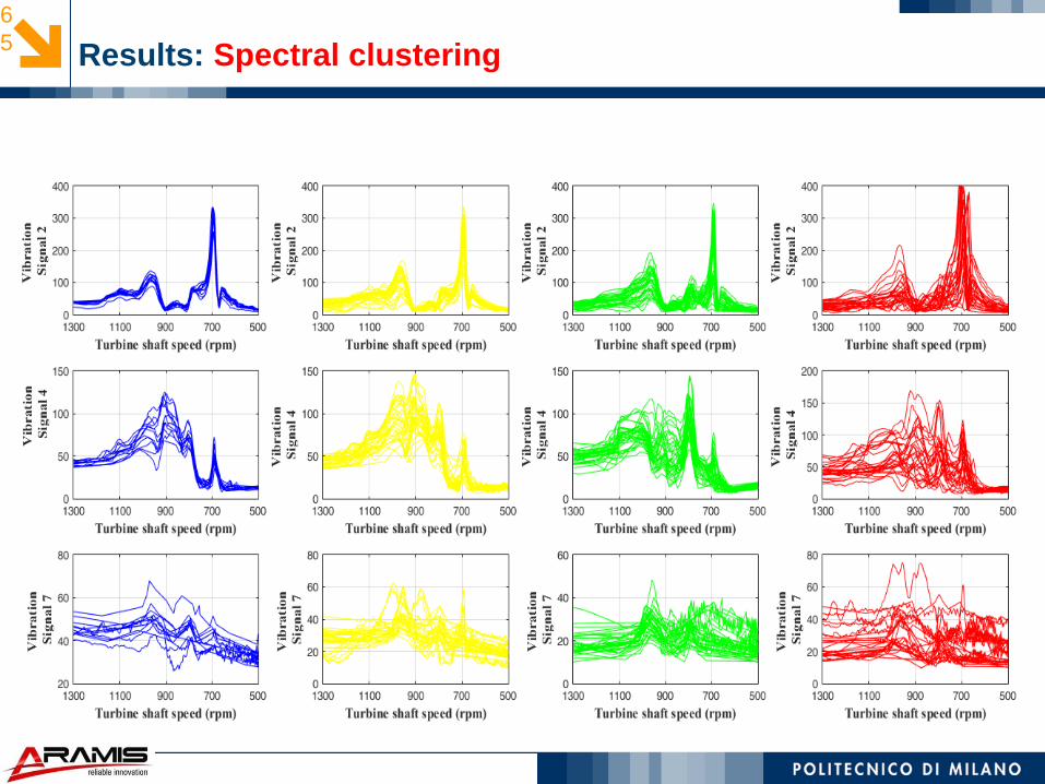
Results: Spectral clustering
6
5

FAULT PROGNOSTICS

Case study: LBE-XADS
The model of the LBE-XADS has been embedded within an MC-driven fault
injection engine to sample component failures.
Dia
ther
mic
oil
tem
per
atu
re
Upper threshold
Lower threshold
“High-temperature failure mode”
“Low-temperature failure mode”
“safe”
4 control/actuator faults
64 accident scenarios
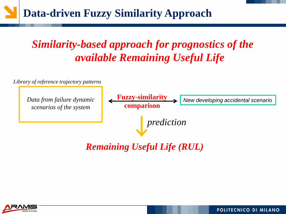
Similarity-based approach for prognostics of the
available Remaining Useful Life
Data-driven Fuzzy Similarity Approach
Remaining Useful Life (RUL)
Data from failure dynamic
scenarios of the system
Library of reference trajectory patterns
New developing accidental scenarioFuzzy-similarity
comparison
prediction

Methodology: Fuzzy Similarity Analysis
1- Trajectory pointwise difference computation:
n-long test trajectory pattern (Fig.1)
n-long , j-th interval of the i-th treference trajectory pattern (Fig. 1)
2- Trajectory pointwise similarity computation:
μ (i,j) is the membership value of the distance
δ (i,j) to the condition of “approximately zero”
3- RULi (t) estimation:
4- RUL estimation:
Weighted sum of the RULi , i=1,2,…,N
RUL =wi ·RULi with i=1,2,…,N
Figure 1

Results

Modern Reliability and Maintenance
Engineering for Modern Industry

Tools for a SMART Reliability and Maintenance
Engineering for Modern Industry
Fuzzy Logic
Systems
Optimization
Algorithms
FTA
ETA
FMECA
Hazop
Clustering
Algorithms
Graph
Theory
Petri Nets
Neural
Networks
Bayesian
Belief
Networks
Complex
Network Theory
Monte Carlo
Simulation
Process and
Stochastic
Flowgraphs