MODELLING, CONTROL AND SIMULATION OF PIEZOELECTRIC SMART ...facta.junis.ni.ac.rs/macar/macar2002/macar2002-10.pdf · Modelling, Control and Simulation of Piezoelectric Smart Structures

FACTA UNIVERSITATISSeries: Mechanics, Automatic Control and Robotics Vol.3, No 12, 2002, pp. 417 - 430

MODELLING, CONTROL AND SIMULATION OFPIEZOELECTRIC SMART STRUCTURES USING FINITE

ELEMENT METHOD AND OPTIMAL LQ CONTROL UDC 62-52:62-50:534:531

Ulrich Gabbert1, Tamara Nestorović Trajkov1,2, Heinz Köppe1

1Otto-von-Guericke-Universität Magdeburg, Fakultät für Maschinenbau,Institut für Mechanik, Universitätsplatz 2, 39106 Magdeburg, Germany

2Faculty of Mechanical Engineering, Beogradska 14, 18000 Niš, Yugoslavia

Abstract. The paper presents some recent developments in modelling and numericalanalysis of piezoelectric material systems and controlled smart structures based on ageneral purpose finite element software with the possibilities of static and dynamicanalyses and simulation. Design and simulation of controlled smart structure is alsopresented, using a state-space model of a structure obtained through the finite elementanalysis as a starting point for the controller design. For the purpose of the controldesign for the vibration suppression discrete-time control design tools were used, suchas optimal LQ controller incorporated in a tracking system. The application ofmentioned methods was verified through the example of actively controlled vibrationsof the clamped beam.

Key words: piezoelectric smart structures, finite element analysis, optimal LQ control,tracking system.

1. INTRODUCTION

An increasing interest in the possibilities of active control of structures has given riseto new achievements in this field of research in many branches of engineering over thepast few years. In comparison with passive structures, smart structures (or activestructures, or structronic systems as they are referred to in different literature) offer agreat variety of possibilities for the structural behavior control under changingenvironment conditions in the sense of adjusting or adapting the structure parameters andbehavior to new conditions. From this point of view the term adaptive structure is alsoused to denote the possibility of altering the structural response in the presence ofdisturbances or changed working conditions. The ability of the structure to change itsresponse in accordance with the changed environment conditions comes from thepresence of active materials integrated with the structure. Such active materials (acting as

Received February 01, 2002

418 U. GABBERT, T. NESTOROVIĆ TRAJKOV, H. KÖPPE

sensor and/or actuators) in connection with the control system enable automaticadaptation of the structure to changing environment conditions. An important role amongactive materials belongs to piezoelectric materials (such as thin wafers, fibers orpiezoelectric rods) used as actuators and sensors integrated in a structure providing thusthe adaptability of the smart structure, while not affecting significantly its passivebehavior. Piezoelectric sensing and control with distributed piezoelectric transducershave been intensively studied, e.g. [6], [16], [19]. Application of piezoelectric materialsin active structural control requires appropriate simulation and design tools. One of suchtools [5] has been developed by the authors (Gabbert et al.) and it represents a generalpurpose finite element based simulation software for piezoelectric smart structures. Thesoftware includes an extensive library of coupled finite elements which cover 1D, 2D and3D continua as well as multilayered composite shell continua based on a generalapproach. The finite element code includes a substructure technique which provides thepossibility of separating mechanical and piezoelectric structures. It also contains a datainterface for the communication between finite element analysis tools and controllerdesign tools such as Matlab/Simulink. Theoretical background of the finite elementsoftware tool COSAR will be briefly presented in the following chapters.

2. BASIC EQUATIONS OF PIEZOELASTICITY

The coupled electromechanical behavior of a polarizable (but not magnetizable)piezoelectric smart material can be described with adequate accuracy with linearizedconstitutive equations. These linear equations can be derived from the energy expression[18] in a quadratic form of the primary field variables: mechanical strain εεεε and electricfield E, on the basis of the assumption that the temperature distribution θ is a prioriknown or can be calculated independently of the electromechanical fields. The potentialfunction [14], [18] can be written in the following form:

θ+θ−−−= πEζεκEEeEεCεεEε TTTTT21

21),(H . (1)

Dependent variables: mechanical stress σσσσ and electric displacement D are derivedfrom (1) by partial differentiation as:

., T θ++=∂∂−=θ−−=

∂∂= πκEεe

EDζeECε

εσ HH (2)

or in the scalar form [11]:

., θ+κ+ε=θλ−−ε=σ εεilillmilmi

Eiklliklm

Eiklmik pEeDEec (3)

Equations (2) can be written in the matrix notation as:

ΘJγΨ −= (4)using the following block-matrices:

θ−θ=

−

=

−

=

=

πζΘ

Eε

γκe

eCJ

Dσ

Ψ ,,, T (5)

Modelling, Control and Simulation of Piezoelectric Smart Structures Using Finite Element Method... 419

where: σσσσT=[σ11 σ22 σ33 σ12 σ23 σ31] is the stress vector, C(6×6) is the symmetric elasticitymatrix, εεεεT=[εεεε11 εεεε22 εεεε33 εεεε12 εεεε23 εεεε31] is the strain vector, e(6×3) is the piezoelectric matrix,ET=[E1 E2 E3] is the electric field vector, ζζζζ is the vector of thermal stress coefficients, θrepresents the temperature variation of the body with respect to the initial temperature,DT=[D1 D2 D3] is the vector of electric displacements, κκκκ(3×3) is the symmetric dielectricmatrix and ππππ is the vector of pyroelectric coefficients.

The linear constitutive equations are an approximation of the real non-linear behavior,which is quite accurate in low electric field applications and gives sufficiently accurateresults in most design processes of engineering smart structures.

The constitutive equations (4) together with the mechanical and electric balanceequations as well as the mechanical and electric boundary conditions represent a uniqueset of equations for the coupled electromechanical problem. Equations of motion writtenin the matrix notation and the charge equation of electrostatics resulting from Maxwell’sequations [17] are respectively:

0DL0upσL ==ρ−+ φTT ,u in V (6)

where [ ]321T ppp=p is the body force vector, uT=[u1 u2 u3] is the vector of

mechanical displacements described in Cartesian coordinates system xT=[x1 x2 x3], ρ isthe mass density and Lu and Lφ are differentiation matrices:

∂∂

∂∂

∂∂

=

∂∂

∂∂

∂∂

∂∂

∂∂

∂∂

∂∂

∂∂

∂∂

= φ

3

2

1

123

312

321T ,

000

000

000

x

x

x

xxx

xxx

xxx

u LL . (7)

Now the balance equations can be represented in a compact form:

0qρbΨL =−+T (8)

where:

φ

=

ρ=

=

=

φ

uq

000I

ρ0p

bL00L

L ,,,u . (9)

The linear strain-displacement relation εεεε = Luu and the relation E = −Lφφ between theelectric field vector E and electric potential φ, can be written together in the form:

LqEε

γ =

−

= . (10)

Taking (10) into account, the constitutive relation (4) can be written in the form:

ΘJLqΨ −= (11)


Now, the balance equation (8) can be written as:

0qρbΘLJLqL =−+− TT , (12)or in the extended form:

0u

000I

0p

θπLθζLu

κLLLeLeLLCLL

=

φ

ρ−

+

−−

φ

− φφφφ

φT

T

TTT

TTu

u

uuu . (13)

The mechanical stress and electric charge boundary conditions are:

0nΨt

ττ =−

=−

Q on Oψ (14)

where t is the prescribed traction vector, Q is the surface charge, and n is a matrix ofdirection cosines which transforms the stresses and electric displacements to thecoordinate system normal to the surface. Over bar denotes prescribed values at aparticular part of the surface. The boundary conditions of mechanical displacements andelectric potential are:

0qq =− on Oq. (15)

In terms of the weighted residual method, a coupled electromechanical functional isprovided by multiplying the balance equation (13) with the vector ][ TT δφδ=δ uqcontaining the virtual displacement δu and virtual electric potential δφ, respectively, andintegrating over the entire domain. As a result we obtain:

0ττquρbΘLJLqLqχ =−δ+−+−δ=δ ∫∫ dOdVtOV

)()( TTTT (16)

or in the scalar form [11]:

0})(){(})(){( ,, =δφ+−δσ−+δφ+δρ−ρ+σ=δχ ∫∫ dOnDQunqdVDuupO

iiijijiV

iiiiijij (17)

It is assumed that the virtual quantities are admissible, and consequently, fulfill theboundary conditions (15). Using partial integration and the Gaussian integral theorem,the following form of the functional can be derived from (16):

0τqΘqLbqJLqqLuρqχ =δ+δ+δ+δ−δ−=δ ∫∫∫∫∫ dOdVdVdVdVtcccc OVVVV

TTTTT )()( (18)

Formulation (18) represents a suitable basis for the development of any type of finiteelement for coupled electromechanical problems.


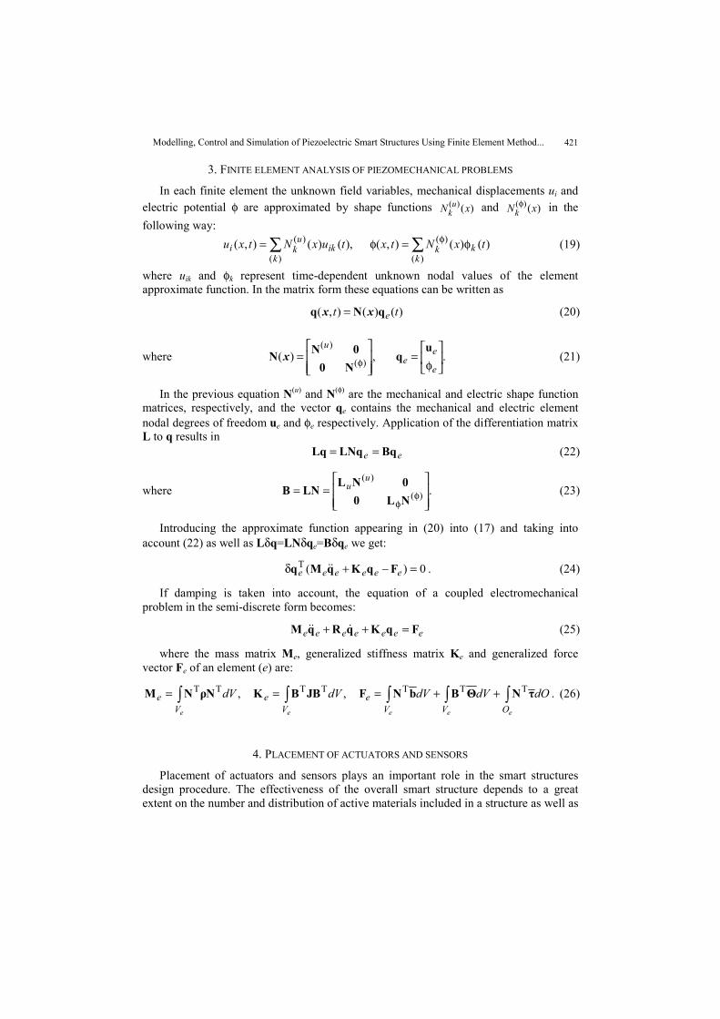
3. FINITE ELEMENT ANALYSIS OF PIEZOMECHANICAL PROBLEMS

In each finite element the unknown field variables, mechanical displacements ui andelectric potential φ are approximated by shape functions )()( xN u

k and )()( xNkφ in the

following way:)()(),(),()(),(

)(

)(

)(

)( txNtxtuxNtxu kk

kikk

uki φ=φ= ∑∑ φ (19)

where uik and φk represent time-dependent unknown nodal values of the elementapproximate function. In the matrix form these equations can be written as

)()(),( tt eqNq xx = (20)

where .,)( )(

)(

φ

=

= φ

e

ee

u uq

N00NN x (21)

In the previous equation N(u) and N(φ) are the mechanical and electric shape functionmatrices, respectively, and the vector qe contains the mechanical and electric elementnodal degrees of freedom ue and φe respectively. Application of the differentiation matrixL to q results in

ee BqLNqLq == (22)

where .)(

)(

== φ

φNL00NL

LNBu

u (23)

Introducing the approximate function appearing in (20) into (17) and taking intoaccount (22) as well as Lδq=LNδqe=Bδqe we get:

0)(T =−+δ eeeeee FqKqMq . (24)

If damping is taken into account, the equation of a coupled electromechanicalproblem in the semi-discrete form becomes:

eeeeeee FqKqRqM =++ (25)

where the mass matrix Me, generalized stiffness matrix Ke and generalized forcevector Fe of an element (e) are:

∫∫∫∫∫ ++===eeeee OVV

eV

eV

e dOdVdVdVdV τNΘBbNFBJBKNρNM TTTTTTT ,, . (26)

4. PLACEMENT OF ACTUATORS AND SENSORS

Placement of actuators and sensors plays an important role in the smart structuresdesign procedure. The effectiveness of the overall smart structure depends to a greatextent on the number and distribution of active materials included in a structure as well as


on the designed controller. On the other hand the actuator/sensor locations affect thecontrollability and the observability of a controlled structure and have a major influenceon the efficiency of the control system and the required control effort to satisfy a givendesign criterion. The placement of actuators/sensors is one of the main problems in thedesign of adaptive structures. In the distributed control of continua (e.g. plate and shellstructures with collocated piezoelectric wafers) the estimation of an optimal actuator andsensor shape as well as their placement are a very complex problem which has not yetbeen fully solved [11].

In the preliminary steps of the smart structure design it is assumed that thespecification of the structure itself, including the objective of the controlled behavior,external disturbances, frequency range etc. is already known. The number and positionsof the required actuators and sensors are roughly estimated in the first approach. This canbe done on the basis of the controllability and observability indices only, where theinfluence of the stiffness and the mass changes due to the active materials as well as thecontroller influence are omitted. Based on the results of an eigenvalue analysis at eachstructural point the modal strains and consequently the modal electric voltage can becalculated which in principal results in the controllability index µk(xP) of the kth mode atthe position xP. The best positions xP to control the first r eigenmodes are those positionswhere the overall controllability index

∏=

µ=µr

kPkkP w

1)()( xx (27)

has the largest value.

5. DEVELOPMENT OF THE STATE-SPACE MODEL AND DATA EXCHANGE

For the purpose of the overall smart structure design and simulation, besides theactive sensor/actuator elements, an appropriate model of the controller is required. Theprocedure of the control law design, testing and verification in the framework of the finiteelement analysis represents in general a complex process which requires some additionaltools to support design process. MATLAB/SIMULINK is a convenient environment for thecontroller design and simulation with many available tools for this purpose and for thatreason it was reasonable to create an interface which would provide data exchangebetween the finite element analysis code and the controller design tool. In this case thisdata exchange should be bi-directional since the data from the finite element model suchas the mass matrix, the stiffness matrix, the damping matrix as well as sensor andactuator positions are required to design the controller and on the other hand thecontroller matrix (or subroutines calculating the controller parameters) is needed in thefinite element package to simulate the controlled structural behavior [11]. For theexchange of data and information between the finite element package COSAR [5] andMATLAB/SIMULINK, a general data exchange interface has been designed andimplemented in the finite element software. The communication concept between thefinite element software COSAR and MATLAB/SIMULINK is shown in Fig. 1.


Finite element system COSAR

Controller Design ToolMatlab/Simulink

FE /C ontrol Interface

Modal State Space Matrices A, B, C, D, E, F

Controller MatrixR

Eigenvalue Analysis

Transient Analysis

Controller Design

Fig. 1. Data exchange between the finite element software COSAR and MATLAB/SIMULINK

Controller design for a flexible mechanical structure represents in general case amultiple input - multiple output (MIMO) problem, where the application of large-scalefinite element models is not suitable due to the high order of the resulting state-spacemodel. Therefore, an appropriate model reduction technique is required to reduce thenumber of the finite element equations. One of the best-known model reductiontechniques is the modal truncation. This technique has been combined with theinvestigations of the dominant behavior of different modes. The modal truncation seemsto be best suited for the controller design of structures based on a finite elementdiscretization, since flexible structures possess a low-pass characteristic, which allowsneglecting high-frequency dynamics. This technique based on the solution of the lineareigenvalue problem

0φMK =λ− kk )( (28)

results in the (n×r) modal matrix ][ 21 rφφφΦ = and the (r×r) spectral matrixΛΛΛΛ = diag(λk), where ΦΦΦΦ is ortho-normalized with ΦΦΦΦTMΦΦΦΦ = I = diag(1) and ΦΦΦΦTKΦΦΦΦ = ΛΛΛΛ.Consequently, inserting the modal coordinates Φxq = into (25) results in a truncatedsystem of r differential equations which can be written as

)()( TT tt uBΦfEΦΛxxΔx +=++ . (29)

Usually, in spite of the system reduction the classical controller design methods in thefrequency domain cannot be applied. Therefore, the controller description is given in thestate-space form. It is assumed that the equation of motion is reduced to the first reigenvectors, which results in (29). Defining the state vector as:

=

xx

z , (30)

the modal reduced model (29) can be transformed into the modal form of the state-spaceequation:

)()()()( TT tttt fEuBzAfEΦ

0u

BΦ0

zΔΛI0

z ++=

+

+

−−

= . (31)

Together with the modal form of the measurement equation

)()( tt fFuDCzy ++= , (32)


which can also be established based on the data of the finite element model, all requiredinformation to design an appropriate controller are prepared. The matrices A, B, C, D, E,F are transferred to MATLAB/SIMULINK via the data interface (Fig. 1) to design thecontroller and to test it through numerical experiments. The controller can also be directlyimplemented on a dSPACE system, which enables designer to work in a hardware-in-the-loop configuration in order to test and modify designed controller on the bases of realexperiments. But before performing such experiments the structural behavior can also betested on a virtual computer model of the structure, which is based on the original finiteelement model. Therefore the controller can be transformed back into the finite elementsoftware via the data interface, where in LTI systems the designed controller matrix L isused to generate the actuator signal as

)()( tt Lyu −= . (33)

The controller can also be directly implemented in the finite element software as C-code subroutine resulting from MATLAB/SIMULINK.

6. CONTROLLER DESIGN

The controller design starts with the continuous state-space model:

duxyduxx

FDCEBA

++=++=

(34)

the state matrices of which are obtained through the finite element analysis and modalreduction described previously. The general form of the plant model (34) assumes thepresence of disturbance d in the state and output equations. Hence, the controller isdesigned introducing additional dynamics [20] to compensate for the presence ofdisturbances and to provide tracking of the reference input with prescribed frequency inorder to suppress vibrations. Additional dynamics is formed based on the assumption thatthe reference input to be tracked and disturbance that acts upon the structure can bedescribed by the rational discrete transfer function. Sine function fulfils this conditionand it is usually used as a disturbance model.

For discrete-time controller design it is necessary to obtain discrete-time state spacemodel of the plant-structure. It is obtained from (34) by discretization with theappropriate sampling time T. Discrete-time model is in the form:

][][][][][][][]1[ kkkkkkkk duxyduxx FDCεΓΦ ++=++=+ (35)

where: .,,00∫∫ τ=τ== ττTT

T dedee EεBΓΦ AAA (36)

Additional dynamics is determined in the state-space form on the basis of disturbanceand/or reference input poles λi. Based on the coefficients of the polynomial:

sss

def

i

mT zzzz ii δ++δ+=−=δ −λ∏ ...)e()( 11 , (37)


obtained by mapping the pole locations into the z-plane, the additional dynamics,described by ΦΦΦΦa and ΓΓΓΓa matrices:

δ−δ−

δ−δ−

=

δ−δ−

δ−δ−

=

−−

s

s

a

s

s

a

1

2

1

1

2

1

,

000100

010001

ΓΓΓΓΦΦΦΦ , (38)

is formed.Discrete-time design model (ΦΦΦΦd, ΓΓΓΓd) is formed as a cascade combination of additional

dynamics (ΦΦΦΦa, ΓΓΓΓa) and discrete-time plant model (ΦΦΦΦ, ΓΓΓΓ) obtained for specified samplingtime T:

xd[k+1] = ΦΦΦΦd xd[k] + ΓΓΓΓd u[k] (39)

where:

=

][][

][kk

ka

d xx

x ,

=

=

0CΓΓΓΓ

ΓΓΓΓΦΦΦΦΓΓΓΓ0000ΦΦΦΦ

ΦΦΦΦ daa

d , . (40)

Feedback gain matrix L of the optimal LQ regulator is calculated on the basis ofdesign model (39) in such a way that the feedback law u[k]= −Lxd[k] minimizes theperformance index:

∑∞

=+=

0])[][][][(

21

k

Td

Td kkkkJ RuuQxx (41)

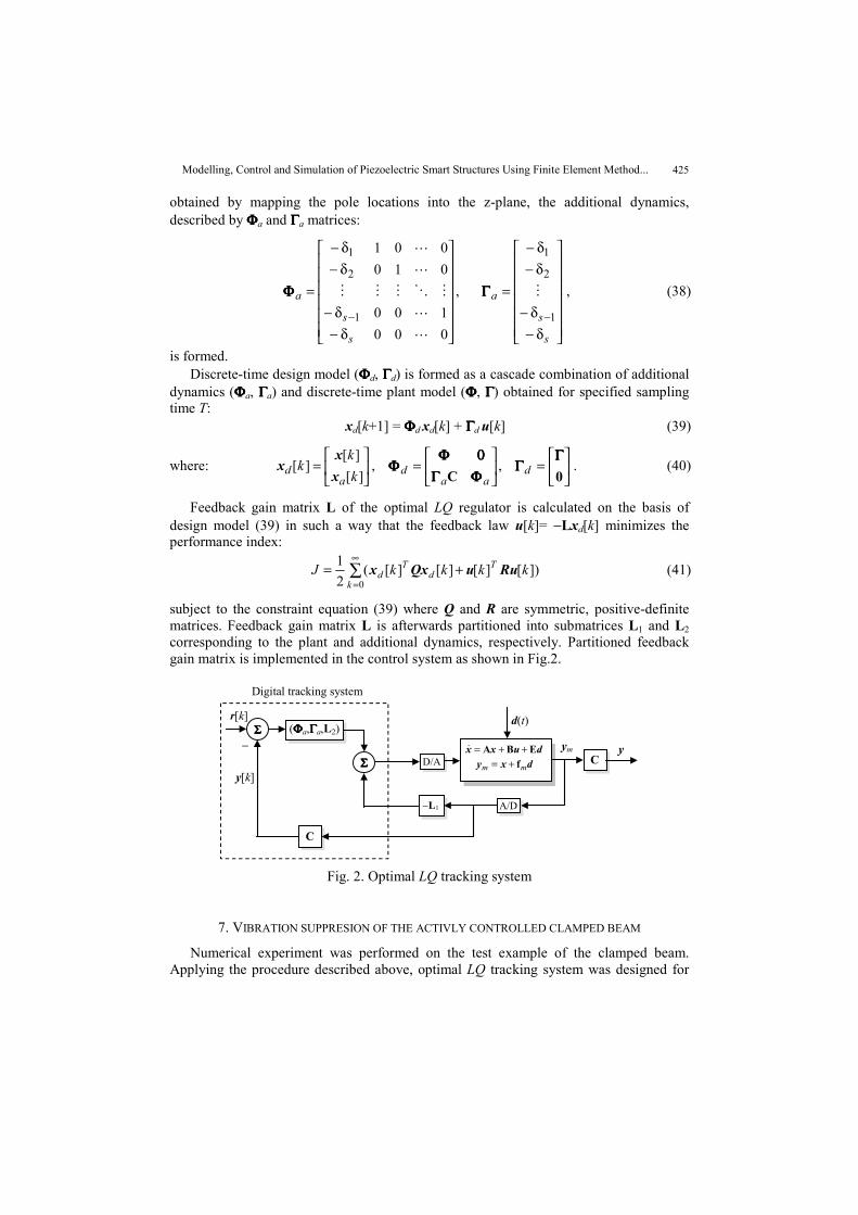
subject to the constraint equation (39) where Q and R are symmetric, positive-definitematrices. Feedback gain matrix L is afterwards partitioned into submatrices L1 and L2corresponding to the plant and additional dynamics, respectively. Partitioned feedbackgain matrix is implemented in the control system as shown in Fig.2.

(ΦΦΦΦa,ΓΓΓΓa,L2)ΣΣΣΣ

−L1

C

r[k]

y[k]D/A

d(t)

Digital tracking system

ym− duxx EBA ++=dxy mm f+=ΣΣΣΣ

A/D

Cy

Fig. 2. Optimal LQ tracking system

7. VIBRATION SUPPRESION OF THE ACTIVLY CONTROLLED CLAMPED BEAM

Numerical experiment was performed on the test example of the clamped beam.Applying the procedure described above, optimal LQ tracking system was designed for


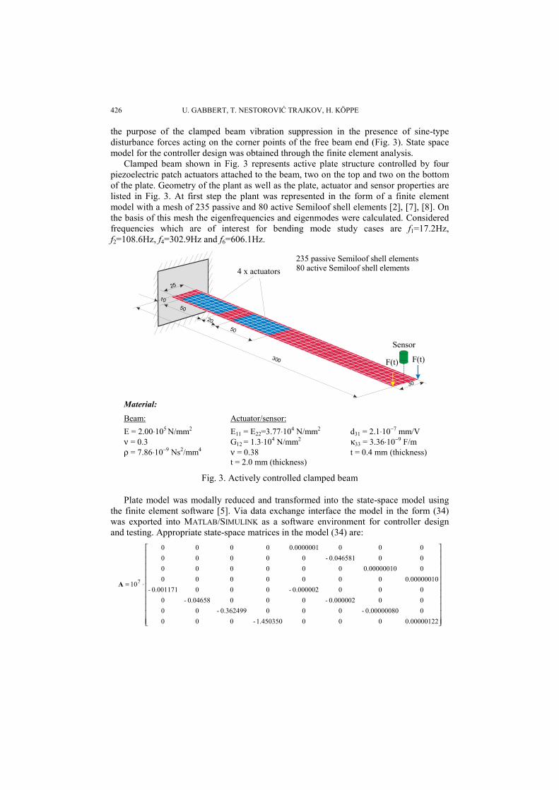
the purpose of the clamped beam vibration suppression in the presence of sine-typedisturbance forces acting on the corner points of the free beam end (Fig. 3). State spacemodel for the controller design was obtained through the finite element analysis.

Clamped beam shown in Fig. 3 represents active plate structure controlled by fourpiezoelectric patch actuators attached to the beam, two on the top and two on the bottomof the plate. Geometry of the plant as well as the plate, actuator and sensor properties arelisted in Fig. 3. At first step the plant was represented in the form of a finite elementmodel with a mesh of 235 passive and 80 active Semiloof shell elements [2], [7], [8]. Onthe basis of this mesh the eigenfrequencies and eigenmodes were calculated. Consideredfrequencies which are of interest for bending mode study cases are f1=17.2Hz,f2=108.6Hz, f4=302.9Hz and f6=606.1Hz.

10

25

50

50

300

30

20

10

4 x actuators

Sensor

F(t)F(t)

235 passive Semiloof shell elements80 active Semiloof shell elements

Material:Beam: Actuator/sensor:E = 2.00⋅105 N/mm2 E11 = E22=3.77⋅104 N/mm2 d31 = 2.1⋅10−7 mm/Vν = 0.3 G12 = 1.3⋅104 N/mm2 κ33 = 3.36⋅10−9 F/mρ = 7.86⋅10−9 Ns2/mm4 ν = 0.38 t = 0.4 mm (thickness)

t = 2.0 mm (thickness)

Fig. 3. Actively controlled clamped beam

Plate model was modally reduced and transformed into the state-space model usingthe finite element software [5]. Via data exchange interface the model in the form (34)was exported into MATLAB/SIMULINK as a software environment for controller designand testing. Appropriate state-space matrices in the model (34) are:

⋅=

0.000001220001.450350-00000.00000080-0000.362499-00000.000002-0000.04658-00000.000002-0000.001171-

0.00000010000000000.00000010000000000.046581-000000000.00000010000

107A


,

6.253134646.253045393.232977813.232977781.11557656-1.11557656-0.181388560.1813885600000000

10,

0.10482390-0.104824081.088613611.08861338-1.21732161-1.217321590.342195420.34219542-0.13713482-0.137134820.137539310.13753931-0.003661870.00366187-0.006083670.00608366-0000000000000000

10 53

⋅=

⋅= EB

[ ] [ ] [ ].00,0000,000004332433.00893192.023953924.054877435.1 ==−= FDC

Exciting forces F(t) = Asin(ωit) = Asin(2πfit), A = 0.01, exerted at the corner points ofthe beam end were chosen according to the eigenfrequencies of interest, considering suchdisturbance as the worst case due to the possibility of the resonance. Since disturbance isa sine function, its s-plane poles are complex conjugate numbers λ1,2=±jωi, where ωi=2πfiand fi are the eigenfrequencies of bending modes.

Following the procedure for the controller design described in the previous section,after implementing the controller, the following simulation results were obtained.

0 0.2 0.4 0.6 0.8 1 1.2 1.4 1.6 1.8 2-0.4

-0.3

-0.2

-0.1

0

0.1

0.2

0.3

0.4

0 1 2 3 4 5 6-0.04

-0.03

-0.02

-0.01

0

0.01

0.02

0.03

0.04

Fig. 4 Fig. 5

0 1 2 3 4 5 6-0.04

-0.03

-0.02

-0.01

0

0.01

0.02

0.03

0.04

0 0.2 0.4 0.6 0.8 1 1.2 1.4 1.6 1.8 2-0.015

-0.01

-0.005

0

0.005

0.01

0.015

Fig. 6 Fig. 7


Simulation results in Fig. 4–7 were obtained for different combinations of the referenceinput and disturbance frequencies. For the purpose of discrete-time control system designsampling interval T=0.0001sec was chosen. Each of the diagrams represents comparison ofthe beam end oscillations without control and with control switched 0.5 sec after thebeginning of the simulation. The vibration suppression is obvious.

Results in Fig. 4 were obtained for the case when the excitation forces have the frequencycorresponding to the first bending mode eigenfrequency, i.e. F=0.01sin(2π⋅17.2t). Referenceinput in this case is the sine signal of the same frequency. Weighting matrices Q and R forthe optimal LQ controller design were chosen in the following way: Q=10−7⋅I10×10, R= I4×4.

For the disturbance force F=0.01sin(2π⋅108.6t), corresponding to the second bendingmode eigenfrequency f2=108.6 Hz, simulation results are shown in Fig. 5. In this case inorder to achieve better vibration suppression as well as the reduction of the oscillationfrequency, the reference input was specified to be F=0.01sin(2π⋅17.2t). Weighting matriceswere chosen in the following way: Q=10−5⋅I10×10, R= I4×4.

Fig. 6 represents results for the excitation forces F=0.01sin(2π⋅302.9t) and referenceinput F=0.01sin(2π⋅17.2t). Weighting matrices are: Q=10−2⋅I10×10, R= I4×4.

The result for the forces F=0.01sin(2π⋅606.1t) and reference input F=0.01sin(2π⋅17.2t)are shown in Fig. 7. Weighting matrices were chosen in the same way as in the previouscase, i.e. Q=10−2⋅I10×10, R= I4×4.

In each of the tested cases the controller performed very good stability margins (uppergain margin greater than 30dB, lower gain margin less than –30dB and phase margin128°), which means that the conroller can be considered robust from the stability marginspoint of view. The vibration suppression was achieved with relatively small control effortin terms of low voltage control signals, which represents a real base for the cotrollerimplementation.

The values of the weighting matrices Q and R affect the settling time of the closed-loop system as well as the oscillation magnitudes during the transient response. Withadoped values of the weighting matrices a trade-off between the settling time and thetrancient magnitudes was achieved in order to obtain satisfying results and avoid pickmagnitudes at the instant when the controller is switched on. Thus presented choice of theweighting matrices represents one possible solution. Of course, with any unknown sine-excitation within the first four eigenfrequencies, the steady-state response of the closed-loop control system would be the same as in shown results for the same weightingmatrices used with different excitation frequencies. Since the choice of weightingmatrices affects the transient behavior after swithcing the controller on, pick magnitudescan be avoided with the controller switched on from the very beginning of the simulation.In this way the same controller can face different excitation frequencies. The simulationsalso showed that with appropriate choice of the reference input in combination withappropriate excitation force, tracking of desired vibration frequencies and magnitudescould also be achieved.

8. CONCLUSION

The procedure for modelling and simulation of smart structures based on a generalpurpose finite element software and numerical analysis of piezoelectric material systemshas been presented in the paper. Discrete-time LQ optimal controller in combination with


additional dynamics tracking system has been proposed for the purpose of smartstructure's vibration suppression. Applied techniques turned out to be very convenientfrom the simulation point of view, both in the sense of modal analysis and controllerdesign and simulation procedure, since the proposed finite element software enables dataexchange between its moduls and controller design tools like MATLAB/SIMULINK.Simulation verification of applied methods through the test-example of a clamped beamshowed successful vibration suppression of the beam end in the presence of the sine-typeexcitation forces with frequencies corresponding to eigenfrequencies of the structure ofinterest. Further steps in development of this field involve ongoing experimentalvalidations using dSpace system together with the studies of advanced test cases (likeplate and shell structures) with special emphasis on the research on the possibilities ofpractical applications, such as vibration control of the car roof, computer tomography etc.

REFERENCES

1. Banks H. T., Smith R. C., Wang Y.: Smart Material Structures: Modelling, Estimation and Control, JohnWiley & Sons, Chichester, Masson, Paris, 1996.

2. Berger H. Köppe H., Gabbert U., Seeger F.: On Finite Element Analysis of Piezoelectric ControlledSmart Structures, in Gabbert U., Tzou H. S., editors: Smart Structures and Structronic Systems, KluwerAcademic Publishers, 2001, pp. 189-196.

3. Berger H., Gabbert U., Köppe H., Seeger F.: Finite Element Analysis and Design of PiezoelectricControlled Smart Structures, Journal of Theoretical and Applied Mechanics, 3, 38, 2000, pp. 475-498.

4. Clark R. L., Saunders W. R., Gibbs G. P.: Adaptive Structures - Dynamic and Control, J. Wiley & Sons,Inc., New York, 1998.

5. COSAR - General Purpose Finite Element Package: Manual, FEMCOS mbH Magdeburg (see also:http://www.femcos.de).

6. Gabbert U., editor: Smart Mechanical Systems – Adaptronics, Fortschr.-Ber. VDI Reihe 11, Nr. 244,Düsseldorf: VDI Verlag 1997.

7. Gabbert U., Berger H., Köppe H., Cao X.: On Modelling and Analysis of Piezoelectric Smart Structuresby the Finite Element Method, Applied Mechanics and Engineering, Vol. 5, No. 1, 2000, pp. 127-142.

8. Gabbert U., Köppe H., Fuchs K., Seeger F.: Modelling of Smart Composites Controlled by ThinPiezoelectric Fibers, in Varadan, V.V., editor: Mathematics and Control in Smart Structures, SPIEProceedings Series, Vol. 3984, 2000, pp. 2-11.

9. Gabbert U., Tzou H. S., editors: Smart Structures and Structronic Systems, Kluwer Academic Publishers,2001.

10. Gabbert U., Weber Ch.-T.: Analysis and Optimal Design of Piezoelectric Smart Structures by the FiniteElement Method, ECCM’99 European Conference on Computational Mechanics, August 31-September3, 1999, München, Germany

11. Köppe H., Berger H., Gabbert U., Seeger F., Finite element analysis and design of smart structuresincluding control, Abschlusskolloquium des Innovationskollegs Adaptive mechanische Systeme, 17.-18.Mai 2001, O-v-G Universität Magdeburg

12. Nestorović T: On the results of investigations of the possibilities for active control of some mechanicalstructures, Otto-von-Guericke-Universität Magdeburg, Preprint des Institutes für Mechanik, IFME2001/1

13. Nestorović Trajkov T, Köppe H., Gabbert U.: Active Vibration Control of the Beam and Plate StructureUsing Optimal Tracking System Based on LQ Controller, Proceedings of the Symposium RecentAdvances in Analytical Dynamics-Control, Stability and Differential Geometry, Mathematical Instituteof Serbian Academy of Science and Art, Belgrade, April 4th 2001, (to be issued)

14. Parkus H., edit.: Electromagnetic Interactions in Elastic Solids, Springer Verlag, Wien, New York, 1979. 15. Preumont A.: Vibration Control of Active Structures: An Introduction, Kluver Academic Publishers,

Dordrecht, Boston, London, 1997. 16. Rao S. S., Sunar M.: Analysis of distributed thermopiezoelectric sensors and actuators in advanced

intelligent structures, AIAA Journal, Vol. 31, No. 7, 1993, pp. 1280-1286 17. Rodellar J., Barbat A. H., Casciati F., editors: Advances in Structural Control, CIMNE Barcelona, 1999.


18. Tiersten H. F.: Linear Piezoelectric Plate Vibration, Plenum Press, New York 1969. 19. Tzou H. S., Anderson G. L.: Intelligent Structural Systems, Kluwer: Academic Publishers, 1993. 20. Vaccaro R. J.: Digital Control: A State-Space Approach, McGraw-Hill, Inc., 1995.

MODELIRANJE, UPRAVLJANJE I SIMULACIJA AKTIVNIHKONSTRUKCIJA SA PIEZOELEKTRIČNIM ELEMENTIMA

PRIMENOM METODA KONAČNIH ELEMENATA IOPTIMALNOG LQ UPRAVLJANJA

Ulrich Gabbert, Tamara Nestorović Trajkov, Heinz Köppe

U radu su predstavljena neka aktuelna dostignuća u modeliranju i numeričkoj analizi sistemasa piezoelektričnim materijalima i aktivnih konstrukcija na osnovu softvera opšte namene zaanalizu metodom konačnih elemenata, koji ima mogućnosti za statičku i dinamičku analizu isimulaciju. Prikazano je projektovanje i simulacija upravljane aktivne strukture, pri čemu je modelobjekta u prostoru stanja, dobijen postupkom analize metodom konačnih elemenata, korišćen kaopolazna osnova za projektovanje kontrolera. U cilju projektovanja upravljanja za prigušenjeoscilacija korišćen je upravljački aparat u diskretnom domenu – optimalni LQ kontroler ukombinaciji sa sistemom praćenja. Primena pomenutih metoda verifikovana je na primeru aktivnogupravljanja oscilacijama konzole.

Documents

MODELLING, CONTROL AND SIMULATION OF PIEZOELECTRIC SMART ...facta.junis.ni.ac.rs/macar/macar2002/macar2002-10.pdf · Modelling, Control and Simulation of Piezoelectric Smart Structures