Embed Size (px)
Citation preview

MODELING THE INTERACTION BETWEEN PASSENGER CARS AND TRUCKS
A Dissertation
by
JACQUELINE MARIE JENKINS
Submitted to the Office of Graduate Studies of Texas A&M University
in partial fulfillment of the requirements for the degree of
DOCTOR OF PHILOSOPHY
August 2004
Major Subject: Civil Engineering

MODELING THE INTERACTION BETWEEN PASSENGER CARS AND TRUCKS
A Dissertation
by
JACQUELINE MARIE JENKINS
Submitted to Texas A&M University in partial fulfillment of the requirements
for the degree of
DOCTOR OF PHILOSOPHY
Approved as to style and content by:
Laurence R. Rilett Rodger J. Koppa (Chair of Committee) (Member) Mark W. Burris Cliff H. Spiegelman (Member) (Member) Paul Roschke (Head of Department)
August 2004
Major Subject: Civil Engineering

iii
ABSTRACT
Modeling the Interaction Between Passenger Cars and Trucks. (August 2004)
Jacqueline Marie Jenkins, Ba.Sc., University of Waterloo;
M.E., Texas A&M University
Chair of Advisory Committee: Dr. Laurence R. Rilett
The topic of this dissertation was the use of distributed computing to improve the modeling of
the interaction between passenger cars and trucks. The two main focus areas were the
development of a methodology to combine microscopic traffic simulation programs with driving
simulator programs, and the application of a prototype distributed traffic simulation to study the
impact of the length of an impeding vehicle on passing behavior.
The methodology was motivated by the need to provide an easier way to create calibrated
traffic flows in driving simulations and to capture vehicle behavior within microscopic traffic
simulations. The original design for the prototype was to establish a two-way, real time
exchange of vehicle data, however problems were encountered that imposed limitations on its
development and use.
The passing study was motivated by the possible changes in federal truck size and weight
regulations and the current inconsistency between the passing sight distance criteria for the
design of two lane highways and the marking of no-passing zones. Test drivers made passing
maneuvers around impeding vehicles that differed in length and speed. The main effects of the
impeding vehicle length were found to be significant for the time and distance in the left lane,
and the start and end gap distances.
Passing equations were formulated based on the mechanics of the passing maneuver and
included behavior variables for calibration. Through a sensitivity analysis, it was shown that
increases in vehicle speeds, vehicle length, and gap distance increased the distance traveled in
the left lane, while increases in the speed difference and speed gain decreased the distance
traveled in the left lane. The passing equations were calibrated using the current AASHTO
values and used to predict the impact of increased vehicle lengths on the time and distance in the
left lane. The passing equations are valuable for evaluating passing sight distance criteria and
observed passing behavior.

iv
DEDICATION
This is dedicated to Derek
Together
We ride out the trials and tribulations
And celebrate the accomplishments
With love

v
ACKNOWLEDGEMENTS
I have spent over five years in College Station, attending Texas A&M University, and there are
many friends, colleagues, and mentors that I have to thank for my success. Their guidance,
encouragement, and support are truly appreciated.
First of all, I thank Dave Richardson for introducing me to the late Daniel Fambro and for
encouraging me to attend Texas A&M University. His continued support over the years is truly
appreciated and I value our friendship.
The next person to thank is Dr. Laurence Rilett for his guidance, tutelage, and general
advise. As my graduate chair, he made an investment in my studies and I surely hope that he is
as pleased with the outcome as I am. I also owe thanks to Dr. Rodger Koppa for introducing me
to the area of human factors, granting me the opportunity to gain some practical experience, and
providing input on this research. In addition, I thank Drs. Cliff Spiegelman and Mark Burris for
their effort and comments. Several other people who I thank for their contributions to this
research are Michael Manser, Ashwin Kekre, Roelof Engelbrecht, Sangita Sunkari, Gary Gandy,
and of course all those test drivers who participated in the passing study.
Along the way, I have met many bright and enthusiastic people who have influenced me and
regardless of whether or not they know they did, I sincerely appreciate their efforts. I thank all
of those professors from civil engineering, industrial engineering, safety engineering, statistics,
psychology, and safety education, with whom I had the pleasure of studying. I also thank all of
those people at the Texas Transportation Institute with whom I had the pleasure of working. I
am enriched with the knowledge that they imparted and I endeavor to share that knowledge with
others.
I also thank the AAA Foundation for Traffic Safety, the Texas Transportation Institute, and
the Southwest Region Transportation University Center for the financial support that I received.

vi
TABLE OF CONTENTS
Page
1 INTRODUCTION...................................................................................................................1
1.1 Background ....................................................................................................................11.1.1 Microscopic Traffic Simulation Programs.......................................................21.1.2 Driving Simulator Programs ............................................................................21.1.3 Distributed Traffic Simulations .......................................................................31.1.4 Passing Maneuver ............................................................................................41.1.5 Current Passing Sight Distance Design Practices ............................................51.1.6 Current No-Passing Zone Marking Practices...................................................51.1.7 Passing Models ................................................................................................51.1.8 Truck Impact....................................................................................................6
1.2 Statement of Problem.....................................................................................................61.2.1 Need a Method to Capture Behavior in Microscopic Traffic Simulation
Programs ..........................................................................................................61.2.2 Need a Method to Create Calibrated Vehicle Flows in Driving
Simulators ........................................................................................................71.2.3 Need to Identify What Impact Trucks Have on Passing Sight Distance..........71.2.4 Need to Classify the Factors that Potentially Impact Passing Sight
Distance ...........................................................................................................71.2.5 Need to Develop a Passing Sight Distance Equation.......................................8
1.3 Research Objectives .......................................................................................................81.4 Research Framework and Methodology.........................................................................9
1.4.1 Literature Review.............................................................................................91.4.2 Framework for Distributed Traffic Simulations ..............................................91.4.3 Combine the Simulation Programs ..................................................................91.4.4 Evaluate the Distributed Traffic Simulation ..................................................101.4.5 Conduct a Simulation Study ..........................................................................101.4.6 Reduce and Analyze Simulation Data ...........................................................101.4.7 Evaluate the Use of the Distributed Traffic Simulation.................................101.4.8 Formulate a Passing Sight Distance Equation ...............................................10
1.5 Organization of the Dissertation ..................................................................................11
2 LITERATURE REVIEW – PART 1.....................................................................................12
2.1 Need a Method to Capture Behavior in Microscopic Traffic Simulation Programs ......................................................................................................................122.1.1 Car Following Algorithms .............................................................................132.1.2 Lane Changing Algorithms............................................................................212.1.3 Passing Algorithms ........................................................................................262.1.4 Stochastic Mechanisms..................................................................................282.1.5 Calibration .....................................................................................................29

vii
Page
2.2 Need a Method to Create Calibrated Vehicle Flows in Driving Simulators ................302.2.1 Autonomous Vehicles....................................................................................312.2.2 Controlled Vehicles .......................................................................................332.2.3 Traffic Simulation Vehicles ...........................................................................34
2.3 High Level Architecture...............................................................................................352.3.1 Federation ......................................................................................................352.3.2 Object Model Template .................................................................................352.3.3 Federates ........................................................................................................362.3.4 Runtime Infrastructure ...................................................................................362.3.5 Previous High Level Architecture Distributed Traffic Simulations ..............37
3 LITERATURE REVIEW – PART 2.....................................................................................39
3.1 Need to Identify What Impact Trucks Have on Passing Sight Distance ......................393.1.1 Passing Sight Distance for Design.................................................................403.1.2 Passing Sight Distances for Marking No-Passing Zones...............................423.1.3 State Statutes..................................................................................................433.1.4 Federal and State Truck Size and Weight Regulations..................................443.1.5 North America Free Trade Agreement ..........................................................453.1.6 Reviews of the Federal Truck Size and Weight Regulations.........................46
3.2 Need to Classify the Factors that Potentially Impact Passing Sight Distance..............473.2.1 Study Methods ...............................................................................................473.2.2 Study Results .................................................................................................49
3.3 Need to Develop a Passing Sight Distance Equation ...................................................523.3.1 Empirical Approach .......................................................................................523.3.2 Theoretical Approach.....................................................................................523.3.3 Passing Models to Predict the Impact of Trucks............................................543.3.4 Future Work...................................................................................................54
4 A METHODOLOGY FOR ADVANCING TRAFFIC SIMULATIONS.............................56
4.1 Step 1: Behavior or Traffic Problem ............................................................................574.1.1 Model Elements .............................................................................................574.1.2 Simulation Output..........................................................................................58
4.2 Step 2: Contributing Simulations. ................................................................................584.3 Step 3: Create Distributed Simulation..........................................................................59
4.3.1 Design Process ...............................................................................................594.3.2 Development Process.....................................................................................614.3.3 Evaluation Process .........................................................................................61
4.4 Step 4: Apply Distributed Simulation ..........................................................................614.5 Benefits of the Methodology........................................................................................62
4.5.1 User Benefits..................................................................................................624.5.2 Developer Benefits.........................................................................................62
5 THE PROTOTYPE ...............................................................................................................64
5.1 Step 1: Behavior or Traffic Problem ............................................................................64

viii
Page
5.1.1 Conceptualization of the Distributed Traffic Simulation...............................655.1.2 Import and Export Capabilities ......................................................................665.1.3 Desired Model Elements................................................................................665.1.4 Desired Simulation Output ............................................................................66
5.2 Step 2: Select VISSIM and DriveSafety ......................................................................675.2.1 Description of VISSIM..................................................................................675.2.2 Description of DriveSafety ............................................................................675.2.3 Model Elements .............................................................................................705.2.4 Simulation Output..........................................................................................725.2.5 Import and Export Capabilities ......................................................................72
5.3 Step 3: Create the Prototype.........................................................................................745.3.1 Vehicle Control..............................................................................................755.3.2 Federation ......................................................................................................755.3.3 RTI Services ..................................................................................................775.3.4 Advanced RTI Services .................................................................................785.3.5 VISSIM Federate ...........................................................................................785.3.6 DriveSafety Federate .....................................................................................805.3.7 Initialization of the Prototype ........................................................................845.3.8 Execution of the Prototype.............................................................................845.3.9 Communication Within the Final Prototype ..................................................855.3.10 Vehicle Position Error....................................................................................89
5.4 Recommendations ........................................................................................................915.4.1 VISSIM..........................................................................................................915.4.2 DriveSafety ....................................................................................................915.4.3 Translator Program ........................................................................................915.4.4 Prototype........................................................................................................92
6 APPLICATION OF THE PROTOTYPE..............................................................................93
6.1 Experimental Design ....................................................................................................936.2 Test Drivers ..................................................................................................................93
6.2.1 Risks...............................................................................................................946.3 Experimental Procedure ...............................................................................................94
6.3.1 Practice Scenario............................................................................................946.3.2 Experimental Scenario ...................................................................................95
6.4 Data Collection.............................................................................................................986.4.1 Impeding and Passing Vehicle Data ..............................................................986.4.2 Opposing Vehicle Data ..................................................................................986.4.3 Surveys, Questionnaires and Interviews ......................................................1026.4.4 Observations ................................................................................................102
6.5 Data Reduction – Conventional Definition ................................................................1036.5.1 Data Exploration ..........................................................................................1056.5.2 Data Summary .............................................................................................107
6.6 Data Analysis – Conventional Definition ..................................................................1086.6.1 Factor Effects Plots ......................................................................................1086.6.2 Analysis of Variance Model ........................................................................1116.6.3 Tests for Interaction of Factor Effects .........................................................112

ix
Page
6.6.4 Tests for Speed Factor Effects .....................................................................1126.6.5 Tests for Length Factor Effects....................................................................113
6.7 Analysis Results – Conventional Definition ..............................................................1146.7.1 Time in the Left Lane ..................................................................................1146.7.2 Distance in the Left Lane.............................................................................1156.7.3 Start Gap Distance .......................................................................................1156.7.4 End Gap Distance ........................................................................................116
6.8 Data Reduction – Alternate Definition.......................................................................1166.8.1 Data Exploration ..........................................................................................1176.8.2 Data Summary .............................................................................................120
6.9 Data Analysis – Alternate Definition .........................................................................1206.9.1 Factor Effect Plots .......................................................................................1206.9.2 Tests for Interaction of Factor Effects .........................................................1226.9.3 Tests for Speed Factor Effects .....................................................................1236.9.4 Tests for Length Factor Effects....................................................................123
6.10 Results of the Data Analysis – Alternate Definition ..................................................1236.10.1 Time in the Left Lane ..................................................................................1246.10.2 Distance in the Left Lane.............................................................................1246.10.3 Start Gap Distance .......................................................................................1246.10.4 End Gap Distance ........................................................................................125
6.11 Comparison of Data Analyses (Conventional and Alternate Definitions) .................1256.12 Nonparametric Analysis .............................................................................................126
6.12.1 Conventional Definition...............................................................................1266.12.2 Alternate Definition .....................................................................................1276.12.3 Results of the Nonparametric Analyses .......................................................127
6.13 Transferability of Results ...........................................................................................1276.13.1 Results Using the Conventional Definition .................................................1286.13.2 Results Using the Alternate Definition ........................................................1296.13.3 Distance Judgments in Real and Simulated Environments..........................1306.13.4 Lateral Position ............................................................................................1306.13.5 Bias in Field Data ........................................................................................131
7 PASSING BEHAVIOR.......................................................................................................132
7.1 Driver Variability .......................................................................................................1327.2 Position of the Passing Vehicle Relative to the Impeding Vehicle ............................132
7.2.1 Start Gap ......................................................................................................1327.2.2 End Gap .......................................................................................................133
7.3 Speed of the Passing Vehicle .....................................................................................1347.3.1 Speed Gain...................................................................................................1347.3.2 Maximum Speed Difference ........................................................................1357.3.3 Exceeding the Speed Limit ..........................................................................136
7.4 Acceleration and Deceleration Behavior....................................................................1377.4.1 Acceleration Duration..................................................................................1397.4.2 Acceleration Magnitude...............................................................................1397.4.3 Discussion....................................................................................................140
7.5 Variability in the Types of Passing Maneuver ...........................................................141

x
Page
7.5.1 Start of the Passing Maneuver .....................................................................1417.5.2 End of the Passing Maneuver ......................................................................143
8 PASSING EQUATION.......................................................................................................148
8.1 Elements of the Passing Maneuver ............................................................................1488.1.1 Assumptions.................................................................................................1488.1.2 Passing Maneuver Variables........................................................................1498.1.3 Element d1....................................................................................................1508.1.4 Element d2....................................................................................................1508.1.5 Element d3....................................................................................................1528.1.6 Element d4....................................................................................................1538.1.7 Total Passing Distance.................................................................................154
8.2 Factors Impacting the Passing Maneuver...................................................................1548.2.1 Classification by Impact ..............................................................................1548.2.2 Incorporating the Factors that Potentially Impact the Passing
Maneuver .....................................................................................................1578.3 Validation...................................................................................................................1578.4 Calibration..................................................................................................................159
8.4.1 AASHTO Data.............................................................................................1598.4.2 Results..........................................................................................................160
8.5 Sensitivity Analysis....................................................................................................1618.5.1 Impeding and Passing Vehicle Speeds.........................................................1618.5.2 Impeding and Passing Vehicle Lengths .......................................................1628.5.3 Gap Distances ..............................................................................................1648.5.4 Speed Difference..........................................................................................1658.5.5 Speed Gain...................................................................................................1678.5.6 Summary......................................................................................................169
8.6 Predicting the Impact of Increasing the Impeding Vehicle Length............................1708.6.1 Passing Sight Distance Design Practices .....................................................1738.6.2 No-Passing Zones Marking Practices ..........................................................173
8.7 Evaluating Passing Behavior......................................................................................175
9 SUMMARY ........................................................................................................................177
9.1 Contributions..............................................................................................................1799.1.1 Methodology................................................................................................1799.1.2 Application...................................................................................................1809.1.3 Passing Equation..........................................................................................180
9.2 Future Research..........................................................................................................1819.2.1 Distributed Computing.................................................................................1819.2.2 Simulation....................................................................................................1819.2.3 Behavior Analysis........................................................................................1829.2.4 Traffic Analysis ...........................................................................................182
REFERENCES .....................................................................................................................183

xi
Page
APPENDIX A GLOSSARY AND ACRONYMS ...............................................................196
APPENDIX B SYMBOLS...................................................................................................198
APPENDIX C STATE STATUTES REGULATING PASSING BEHAVIOR ..................199
APPENDIX D INSTITUTIONAL REVIEW BOARD APPROVALS ...............................201
APPENDIX E ORDERING COMBINATION SCHEDULE..............................................203
APPENDIX F SIMULATOR SICKNESS QUESTIONNAIRE .........................................204
APPENDIX G SIMULATOR SICKNESS DATA ..............................................................205
APPENDIX H INFORMED CONSENT .............................................................................206
APPENDIX I INSTRUCTIONS.........................................................................................208
APPENDIX J SUMMARY OF PASSING DATA – CONVENTIONAL
DEFINITION...............................................................................................209
APPENDIX K SUMMARY OF PASSING DATA – ALTERNATE DEFINITION..........211
APPENDIX L PASSING DATA USED TO VALIDATE THE PASSING
EQUATION.................................................................................................214
APPENDIX M VALIDATION RESULTS ..........................................................................216
VITA .....................................................................................................................218

xii
LIST OF TABLES
Page
TABLE 3.1. Passing Sight Distance Values for Design.............................................................. 40 TABLE 3.2. Elements of the Passing Sight Distances for Design .............................................. 42 TABLE 3.3. Minimum Passing Sight Distances for Marking..................................................... 43 TABLE 3.4. Comparison of Truck Size and Weights ................................................................. 46 TABLE 5.1. VISSIM Import Data .............................................................................................. 73 TABLE 5.2. VISSIM Export Data .............................................................................................. 73 TABLE 5.3. DriveSafety Export Data......................................................................................... 74 TABLE 5.4. DriveSafety Import Data......................................................................................... 74 TABLE 6.1. Reported Severity of Simulator Sickness Symptoms ............................................. 94 TABLE 6.2. Linear Regression Equations of Opposing Vehicle Trajectories .......................... 100 TABLE 6.3. Linear Regression Equations of Impeding Vehicle Trajectories .......................... 101 TABLE 6.4. Vehicle Lengths and Widths................................................................................. 101 TABLE 6.5. Normality Test Results for Time, Distance, and Gap Distances, N=64 ............... 105 TABLE 6.6. Normality Test Results for Time, Distance, and Gap Distances, N=63 ............... 107 TABLE 6.7. Time, Distance, and Gap Distances – Conventional Definition ........................... 107 TABLE 6.8. ANOVA Table for a Two-Factorial Experiment with Repeated Measures.......... 111 TABLE 6.9. Interaction of Effects – Conventional Definition ................................................. 112 TABLE 6.10. Effect of the Impeding Vehicle Speed – Conventional Definition ..................... 113 TABLE 6.11. Effect of the Impeding Vehicle Length – Conventional Definition ................... 114 TABLE 6.12. Normality Test Results for Time, Distance, and Gap Distances, N=96 ............. 117 TABLE 6.13. Normality Test Results for Time, Distance, and Gap Distances, N=92 ............. 119 TABLE 6.14. Time, Distance, and Gap Distances – Alternate Definition................................ 119 TABLE 6.15. Interaction of Effects – Alternate Definition ...................................................... 122 TABLE 6.16. Effects of the Impeding Vehicle Speed – Alternate Definition .......................... 123 TABLE 6.17. Effects of the Impeding Vehicle Length – Alternate Definition......................... 123 TABLE 6.18. Comparison of Results – Conventional and Alternate Definitions..................... 125 TABLE 6.19. Nonparametric Results Using the Conventional Definition ............................... 126 TABLE 6.20. Nonparametric Results Using the Alternate Definition ...................................... 127 TABLE 6.21. Comparing the Conventional Definition Results with Field Observations......... 128

xiii
Page
TABLE 6.22. Comparing the Alternate Definition Results with Field Observations ............... 129 TABLE 7.1. Regression ANOVA Results ................................................................................ 143 TABLE 7.2. Pearson Correlation Matrix for Deceleration Behavior. ....................................... 146 TABLE 8.1. AASHTO Design Values for t2 and d2.................................................................. 160 TABLE 8.2. Model Calibration Results .................................................................................... 160 TABLE 8.3. Summary of Responses to Increases in Model Variables ..................................... 169 TABLE 8.4. Marginal Changes in t2 and d2 for Total Vehicle Length...................................... 172

xiv
LIST OF FIGURES
Page
FIGURE 2.1. A notation for the car following theories. ............................................................. 13 FIGURE 2.2. A schematic of the situation at the beginning of a lane change maneuver............ 21 FIGURE 2.3. A schematic of the situation at the beginning of a passing maneuver................... 26 FIGURE 2.4. The interface between federates and the RTI........................................................ 36 FIGURE 3.1. A schematic of the passing maneuver. .................................................................. 39 FIGURE 3.2. The elements of the passing maneuver. ................................................................ 41 FIGURE 3.3. Classifying the passing condition factors by the source........................................ 49 FIGURE 4.1. The general framework for advancing simulations............................................... 56 FIGURE 5.1. A conceptualization of the distributed traffic simulation...................................... 65 FIGURE 5.2. A schematic of the driving simulator at the Texas Transportation Institute. ........ 68 FIGURE 5.3. A sample of the acceleration capabilities of DriveSafety. .................................... 69 FIGURE 5.4. A sample of the deceleration capabilities of DriveSafety. .................................... 70 FIGURE 5.5. The design of the HLA-based prototype. .............................................................. 76 FIGURE 5.6. Depiction of the object classes in the federation................................................... 76 FIGURE 5.7. The RTI interfaces in the developed federation .................................................... 77 FIGURE 5.8. Data output from VISSIM..................................................................................... 79 FIGURE 5.9. Data output from the VISSIM API. ...................................................................... 80 FIGURE 5.10. Processing EntitySetRoadwayVelocity commands in DriveSafety .................... 81 FIGURE 5.11. Data processing through the translator program. ................................................ 82 FIGURE 5.12. The data files that were available to evaluate the federation............................... 85 FIGURE 5.13. A depiction of the comparing the time in the output files................................... 86 FIGURE 5.14. Number of vehicle instances recorded in the VISSIM.fzp file. .......................... 87 FIGURE 5.15. Number of vehicle instances recorded in the API.txt file. .................................. 88 FIGURE 5.16. Number of vehicle instances recorded in the Tranlstor.txt file. .......................... 88 FIGURE 5.17. Number of vehicle instances recorded in the DriveSafety.html file. .................. 89 FIGURE 5.18. The vehicle position error. .................................................................................. 90 FIGURE 6.1. Schematic of the practice scenario with a sample center screen image. ............... 95 FIGURE 6.2. Schematic of the experimental scenario with sample center screen images. ........ 96 FIGURE 6.3. Illustration of the two platoons of impeding vehicles. .......................................... 97

xv
Page
FIGURE 6.4. Coordinates of the location triggers. ..................................................................... 99 FIGURE 6.5. Estimated trajectories of the opposing vehicle using location trigger data. .......... 99 FIGURE 6.6. Histogram of the response variable, time in the left lane. ................................... 106 FIGURE 6.7. Histogram of the response variable, distance in the left lane. ............................. 106 FIGURE 6.8. Factor effects plot for time in the left lane. ......................................................... 109 FIGURE 6.9. Factor effects plot for distance in the left lane. ................................................... 109 FIGURE 6.10. Factor effects plot for start gap distance. .......................................................... 110 FIGURE 6.11. Factor effects plot for end gap distance. ........................................................... 110 FIGURE 6.12. Box plots of start gap distances......................................................................... 118 FIGURE 6.13. Box plots of end gap distances. ......................................................................... 118 FIGURE 6.14. Alternate factor effects plot for time in the left lane. ........................................ 120 FIGURE 6.15. Alternate factor effects plot for distance in the left lane. .................................. 121 FIGURE 6.16. Alternate factor effects plot for start gap distances........................................... 121 FIGURE 6.17. Alternate factor effects plot for end gap distances. ........................................... 122 FIGURE 7.1. Frequency distribution of the start gap distances. ............................................... 133 FIGURE 7.2. Frequency distribution of the end gap distances. ................................................ 134 FIGURE 7.3. The frequency distribution of the speed gain of the passing vehicle. ................. 135 FIGURE 7.4. The frequency distribution of the maximum speed differences. ......................... 136 FIGURE 7.5. The frequency distribution of passing vehicle maximum speeds........................ 137 FIGURE 7.6. The order tasks were performed during the passing maneuvers. ........................ 138 FIGURE 7.7. Frequency distribution of the duration of acceleration. ...................................... 139 FIGURE 7.8. Frequency distribution of the magnitude of acceleration. ................................... 140 FIGURE 7.9. Relative speed (Spi(accel)) versus speed gain (∆sp). ........................................... 142 FIGURE 7.10. Clearance versus relative position at the moment of deceleration. ................... 145 FIGURE 7.11. Lane occupied at the moment of deceleration................................................... 145 FIGURE 8.1. Elements of the passing maneuver. ..................................................................... 148 FIGURE 8.2. Distances traveled during t1................................................................................. 150 FIGURE 8.3. Distances traveled during t2................................................................................. 151 FIGURE 8.4. The clearance distance. ....................................................................................... 153 FIGURE 8.5. Distance traveled by opposing vehicle................................................................ 153 FIGURE 8.6. Classifying passing condition factors by the type of impact............................... 155 FIGURE 8.7. Estimation error for t2.......................................................................................... 158

xvi
Page
FIGURE 8.8. Estimation error for d2......................................................................................... 159 FIGURE 8.9. Sensitivity to the impeding and passing vehicle speeds...................................... 162 FIGURE 8.10. Sensitivity to the total vehicle length. ............................................................... 163 FIGURE 8.11. Sensitivity to the impeding and passing vehicle lengths and speeds. ............... 163 FIGURE 8.12. Sensitivity to the total gap distance................................................................... 164 FIGURE 8.13. Sensitivity to the total gap distance and vehicle speeds. ................................... 165 FIGURE 8.14. Sensitivity to the speed difference. ................................................................... 166 FIGURE 8.15. Sensitivity to the speed difference and impeding vehicle speed. ...................... 167 FIGURE 8.16. Sensitivity to the speed gain.............................................................................. 168 FIGURE 8.17. Sensitivity to the speed gain and vehicle speeds. .............................................. 168 FIGURE 8.18. Sensitivity to gain rate and vehicle lengths. ...................................................... 171 FIGURE 8.19. Predicted impact of vehicle length on AASHTO design values. ...................... 171

1
1 INTRODUCTION
The topic of this dissertation was the use of distributed computing to improve the modeling of
the interaction between passenger cars and trucks. There were two main areas of focus for this
research. The first focus area was the development of a methodology to combine microscopic
traffic simulation programs with driving simulator programs. This was motivated by the current
capabilities of such programs and the potential to increase their usefulness through the
development and application of distributed simulations. A distributed traffic simulation,
combining a traffic simulation and a driving simulation, would provide a way to create specific
traffic flows in the driving simulation and capture both driver and traffic data simultaneously,
thus allowing the interactions between vehicles, the roadway, and the environment to be
investigated. The results could be utilized to improve how vehicle movements are modeled in
simulations.
The second focus area was the application of a distributed traffic simulation. The specific
application was the problem of predicting how the length of an impeding vehicle impacts the
passing behavior of drivers and was taken into account during the creation of a prototype
distributed traffic simulation. Investigation into this problem was motivated by the existing
inadequacies of the passing sight distance design criteria and the current no-passing zone
marking practices which may be exacerbated by a future increase in the federal regulations on
truck weights and sizes. The results were used to develop a passing distance equation that was
based on the mechanics of the maneuver and included behavior variables. This equation could
be used to evaluate passing sight distance criteria and passing behavior observed in the field.
1.1 Background
To understand the motivations behind the first area of focus, the capabilities of microscopic
traffic simulation programs and driving simulator programs were reviewed along with the
current High Level Architecture (HLA) standards used to guide the creation of distributed
simulations. To understand the motivations behind the second area of focus, the current passing
sight distance criteria were reviewed along with the history of passing studies. These literature
This dissertation follows the style and format of the Transportation Research Record.
2
reviews are summarized in the following sections and comprehensively detailed in Sections 2
and 3.
1.1.1 Microscopic Traffic Simulation Programs
A microscopic traffic simulation model is a simplified description of a traffic system that
includes details about the traffic network, traffic controls, and the movement of individual
vehicles. Theories of car following and lane changing that explain the fundamental relationships
between vehicles and the interaction with traffic controls under specific roadway environments
are derived from facts, conjecture, reasoning, speculation, and supposition. These theories are
the basis of the program logic controlling the movement of vehicles. Dynamic, stochastic
models are capable of mimicking complex traffic systems and are studied through simulation.
The general acceptance and popularity of traffic simulation programs is evident by the
inclusion of a chapter on simulation and other models in the 2000 version of the Highway
Capacity Manual (1). In a review conducted in 1997 (2), fifty-seven existing microscopic traffic
simulation programs were identified that were used to simulate the operation of intersections,
urban street networks, freeways, integrated networks, et cetera.
Microscopic traffic simulation programs are used to evaluate and optimize traffic systems,
predict the impact of changes, evaluate alternatives, and conduct sensitivity analyses. They
model individual vehicles and have the ability to simulate sophisticated vehicle movements,
however their ability to model complex behavioral aspects are limited.
Many programs output statistics on the operation of the traffic system being simulated, such
as delays, travel times, level of service, etc., but provide little information about driver behavior.
In fact, parameters used to calibrate the simulation reflect the behavior of drivers in the system
but rarely have a direct interpretation.
It is becoming common for microscopic traffic simulation programs to include some sort of
visualization capability to view the traffic simulation. This capability provides the means to
visually verify that the simulation is behaving as expected and to identify where operational
problems are occurring in the simulated network.
1.1.2 Driving Simulator Programs
Driving simulators have developed as a visualization tool and have been used for driver training
and driving research including perceptual, cognitive, and behavioral studies. Test drivers control
a vehicle in a computer generated driving environment and details about the test drivers’ control

3
of the vehicle are captured. The use of driving simulators has grown as illustrated by the variety
of commercial systems available as well as the variety of driving simulators that continue to
develop through independent research efforts. INRETS maintains a listing of driving simulators
that currently includes over fifty research simulators and twenty training simulators from around
the world (3).
Driving simulators are an attractive alternative to field and course testing as the test drivers
are in a safe and highly controlled driving environment. The human-in-the-loop nature of the
apparatus allows the stochastic and dynamic nature of driver behavior to be captured. In
addition, personal contact with the test drivers provides the opportunity to administer detailed
questionnaires about the test drivers’ driving habits, experience, health, et cetera.
One of the issues in developing driving simulators is how to create traffic that can behave
autonomously and at the same time have traffic that can be specifically controlled to create a
highly orchestrated traffic environment. So far, a combination of scripted vehicles, which are
programmed to behave in a predetermined fashion, and ambient traffic, which is made up of
randomly generated vehicles that act as background traffic to add a sense of realism to the
driving environment have been used. Generally, vehicles move according to some vehicle
attributes such as the acceleration, speed, headway, tailway, et cetera. While these techniques
are suitable for creating a driving scenario with relatively few vehicles, problems arise when
specific, or calibrated traffic flows are desired or when the movement of vehicles needs to mimic
real car following and lane changing behavior.
The output from driving simulator programs is largely focused on measures of driver
behavior and vehicle control. Little information is available about the traffic environment being
modeled. This limitation can be problematic when details about the traffic or the movement of a
group of vehicles are required. For instance, to conduct a gap acceptance study the spacing
between consecutive vehicles is needed.
1.1.3 Distributed Traffic Simulations
The main advantage of distributed computing is the flexibility of combining a variety of
disparate simulations while maintaining the integrity of the individual simulations. In a
distributed traffic simulation, a number of traffic simulations are combined to run together taking
advantage of the strengths of the individual simulations. Information about vehicle movements,

4
traffic controls and other dynamic entities can be communicated between the individual
simulations.
A distributed traffic simulation that combines a microscopic traffic simulation with a driving
simulator could be used to investigate the interaction between passenger cars and trucks for a
variety of driving behaviors such as car following, lane changing, and passing under a variety of
traffic environments since both driver and traffic data could be recorded simultaneously. Driver
behavior studies could be conducted using a traffic simulation that is calibrated to existing or
predicted future traffic conditions. The results of these studies could be used to improve
understanding of driver behavior and used to enhance the traffic models used in the simulation.
The distributed traffic simulation also allows researchers to view traffic simulations from
anywhere in the network from the driver’s point of view and, if desired, the driver could interact
with the simulated traffic and vice versa.
Distributed traffic simulation is also beneficial for both traffic simulation program
developers and driving simulator developers. Each could focus on developing the strengths of
their programs and by meeting certain design considerations, could contribute to a distributed
traffic simulation. Programs could be specific to a type of transportation investigation, type of
facility, type of vehicle, or method of visualization and would not have to provide all capabilities
for all uses. Developers could then direct future research and development of their programs to
meet the specific needs of particular user groups and to provide the capabilities needed for
distributed traffic simulation. Intuitively, the ability to model background traffic using a
previously calibrated and validated microscopic traffic simulation model would allow driving
simulator developers to concentrate on developing advanced visualization software and vehicle
dynamics models. Likewise, having access to powerful visualization tools would allow
microscopic traffic simulation program developers to concentrate on improving how the traffic
network, traffic controls, and the movement of individual vehicles are modeled.
1.1.4 Passing Maneuver
One of the more complicated and inherently dangerous driving tasks is the passing maneuver. A
driver uses the opposing lane to accelerate around an impeding vehicle while providing enough
space to prevent colliding with the impeding or opposing vehicles. Driver behavior is a function
of the atmospheric, roadway and traffic conditions, the performance capabilities of the vehicle,
and the skills and attitudes of the driver.

5
1.1.5 Current Passing Sight Distance Design Practices
In the 1930’s a significant effort was made to collect passing data in the field (4, 5, 6, 7).
Observations were made from fixed points or test vehicles and speedometers, stopwatches,
cameras, and markings and/or detectors on the road were used to measure and/or record the
observations with varying success. The Holmes method (8) was used to collect data for over
20,000 passes and Prisk (9) extracted 3,521 simple passes with a delayed start and a hurried
return for analysis. This analysis set the foundation for the passing sight distance values given in
the American Association of State Highway and Transportation Officials (ASSHTO) publication
A Policy on Geometric Design of Highways and Streets (10, 11).
1.1.6 Current No-Passing Zone Marking Practices
The ASSHTO passing sight distance values are much larger than those found in the Manual on
Uniform Traffic Control Devices (12) used for marking no-passing zones. These latter values
were developed as a compromise between the sight distances needed for a flying pass and a
delayed pass. They were also a compromise between safety and making excessive restrictions
on passing, such that safety would require good driver judgment. Although it is not clear where
these numbers originated, they can be traced as far back as the 1940 AASHTO publication A
Policy on Criteria for Marking and Signing No-Passing Zones on Two and Three Lane Roads
(13).
1.1.7 Passing Models
Over the years, a number of models have been developed to describe the passing maneuver. In
1972, Herman and Lam (14) developed an analytical model of the passing maneuver and
proposed the idea that there exists a point of no return where the driver is better to complete
rather than abort the maneuver. A decade later, Lieberman (15) developed an analytic model
based on the kinematics of the passing maneuver and described the critical position as the
moment that completing or aborting the passing maneuver would offer the driver the same
clearance with oncoming vehicles. The idea of a critical point or a point of no return was
adopted by numerous authors (16, 17, 18, 19) and their passing models were used to evaluate the
AASHTO passing sight distance design values and the MUTCD no-passing zone marking
values, both of which consider a passenger car passing another passenger car. Assumptions were
made about the values of the head-on clearance, gap size, deceleration rate, and speed

6
differential. Some of the passing models were also used to predict the impact of trucks on the
needed passing sight distance.
1.1.8 Truck Impact
By varying the vehicle length used in the passing models, it was predicted that when a truck was
being passed, the needed passing sight distance was greater (15, 16, 18, 20, 21). This result was
a consequence of how the vehicle length was taken into account in the models. For instance, in
the Lieberman (15) and Saito (16) models, the increase in passing sight distance reflected the
increased distance the passing vehicle needed to travel along the length of the impeding vehicle.
However, in the Glennon model, the result was amplified by the speed of the impeding vehicle
(20).
In 2000, Polus, Livneh and Frischer (22) aimed to quantify the major components of the
passing maneuver by examining approximately 1,500 passing maneuvers videotaped from
vantage points and from a hovering helicopter. The speed differential, headway between the
passing and impeding vehicles at the beginning of the maneuver, distance the opposing lane was
occupied, tailway between the passing and impeding vehicles at the end of the maneuver, and
clearance to the opposing vehicle were observed to be greater when the impeding vehicle was a
tractor semi trailer. This result suggested that the impact of an increase in the impeding vehicle
length was not limited to the added distance traveled along the length of the impeding vehicle,
and that the passing behavior of the driver differed depending on the type of impeding vehicle.
Understanding what impact trucks have on passing sight distance is important because there
are currently pressures on the United States to increase the allowable federal truck length limits
to compare with those of Canada and Mexico. To permit the use of longer trucks, it is
imperative that the current design practices and no-passing zone marking practices will be
adequate.
1.2 Statement of Problem
1.2.1 Need a Method to Capture Behavior in Microscopic Traffic Simulation Programs
Microscopic traffic simulation programs are developed for engineering analyses. These models
are very good at modeling traffic flows and produce measures of effectiveness describing the
operation of the traffic system. Traffic conditions are calibrated by adjusting the values of
behavioral parameters. Unfortunately, these values generally have no direct interpretation. To

7
gain driver behavior data, studies in the field, on a test track, or using a driving simulator are
conducted. These types of studies have their own limitations including cost, risk, and the type
and quality of data that can be collected. What is needed is a method to introduce a test driver
into the microscopic traffic simulation that has calibrated traffic conditions so that driver
behavior data can be captured in a safe and efficient manner.
1.2.2 Need a Method to Create Calibrated Vehicle Flows in Driving Simulators
Driving simulators are developed for driver training and behavior research. Test drivers control
a vehicle in a computer generated driving environment and measures of their control of the
vehicle are recorded. To create the traffic conditions, individual vehicles are specifically
programmed and ambient traffic is included to provide a sense of realism. Calibrating the traffic
conditions may require each vehicle in the simulation to be specifically programmed, which
would be a time consuming and laborious task. An easier method to create a specific or
calibrated traffic flow is needed.
1.2.3 Need to Identify What Impact Trucks Have on Passing Sight Distance
A number of models have been developed and applied to determine whether longer impeding
vehicles require greater passing sight distances. The models were used to predict that greater
passing sight distance is required when longer impeding vehicles are passed. However, the
predictions reflected how the vehicle length was taken into account in the development of the
models. A recent field study was conducted and the results suggested that the impact of longer
vehicles was not limited to the length of the vehicle. What is needed is to identify what impact
trucks have on the needed passing sight distance.
The limitations of traditional data collection methods for field studies, test track studies, and
driving simulator studies include cost, risks, and the type and quality of data. What is needed is
an alternate method that allows both traffic and driver data to be collected in a safe and
controlled driving environment at a reasonable cost to determine whether longer impeding
vehicles influence the mechanics of the passing maneuver and/or the passing behavior of drivers.
1.2.4 Need to Classify the Factors that Potentially Impact Passing Sight Distance
Passing behavior is highly variable, resulting from the influences of the environment and the
capabilities of the vehicles and drivers. It is not realistic or practical to include every factor
when building a model to describe the needed passing sight distance. What is needed is a

8
classification of factors to identify which factors have the potential to impact the mechanics of
the passing maneuver and/or the passing behavior of drivers.
1.2.5 Need to Develop a Passing Sight Distance Equation
Numerous models have been developed describing the mechanics of the passing maneuver but
most are based on the concept of a point of no return or a critical point, which has not been
validated. What is needed is an equation for the passing distance that is based on the mechanics
of the passing maneuver and also has behavior parameters for calibration.
1.3 Research Objectives
It was hypothesized that the traffic modeling capabilities of microscopic traffic simulation
programs and the visualization capabilities of driving simulation programs could be exploited by
combining the disparate programs into a distributed traffic simulation. The combined simulation
could then be used to capture driver behavior and traffic data simultaneously for a variety of
driver behaviors in a variety of traffic environments and the results applied to improve the
current traffic models. The objectives of this research were to:
1. Develop a general methodology to combine microscopic traffic simulation programs
with driving simulator programs, providing an easier way to create calibrated traffic
flows in driving simulators and to capture vehicle behavior in microscopic traffic
simulation programs;
2. Evaluate the benefits and drawbacks of this methodology;
3. Apply the distributed traffic simulation to study the passing maneuver, as an alternative
study method to the costly and dangerous field study;
4. Classify the factors that have the potential to impact passing sight distance; and
5. Formulate a passing equation that describes the mechanics of the maneuver and includes
behavior parameters. This equation could be used to improve the logic used by both
microscopic traffic simulation programs and driving simulator programs.
The methodology was intended to be developed in a generalized manner such that it could be
applied to a variety of driver behaviors and traffic environments. Pedestrian movements and the
operation of traffic control devices were outside the scope of this research.

9
1.4 Research Framework and Methodology
This research was divided into eight tasks. The purpose and description of each task is presented
in the following sections.
1.4.1 Literature Review
The first task was to perform a comprehensive literature review on the aspects of combining
traffic simulation programs. Passing literature was also reviewed, including the data collection
methods used to capture passing maneuver data, models that have been developed, and
behavioral studies that have been conducted. This review reflected the multidisciplinary nature
of this research, drawing from simulation, distributed computing, transportation, human factors,
and psychology publication sources. The purpose of the literature review was to ensure that no
research, which might contribute to this study, was overlooked or unnecessarily duplicated.
1.4.2 Framework for Distributed Traffic Simulations
The second task was to develop a general framework that outlined the methodology for creating
and applying a distributed traffic simulation and the avenues for feedback to improve the
individual simulations, the distributed traffic simulation, and understanding of the particular
application.
1.4.3 Combine the Simulation Programs
The third task was to use the general framework to guide the design and development of a
distributed traffic simulation. High Level Architecture was adopted to combine a microscopic
traffic simulation with a driving simulation. Issues concerning the exchange of data, consistency
in the meaning of data, and synchronization were expected (23). Each of these issues was
addressed in this research.
A cursory look at the capabilities of the microscopic traffic simulation program VISSIM (24)
and the DriveSafety (25) driving simulator located at the Texas Transportation Institute, which
were both proprietary programs, suggested that combining them was feasible. VISSIM had an
External Driver Application Programming Interface (API) that could be used to control vehicles
in the traffic simulation from an external source. DriveSafety used Transmission Control
Protocol/Internet Protocol (TCP/IP) to transfer information through sockets.

10
1.4.4 Evaluate the Distributed Traffic Simulation
The fourth task was to evaluate the distributed traffic simulation. A review of some recent
simulation publications revealed that distributed traffic simulations have previously been
developed based on HLA (26, 27), including one for simple urban traffic. The developers noted
that there was no noticeable slowdown in the animation but slowdown could occur if larger
traffic networks were modeled. For this research, the distributed traffic simulation was
evaluated to verify that it was working as expected and that performance levels were acceptable,
including the data transfer processes and the quality of the animation. The evaluation results
were used to construct recommendations for improvements.
1.4.5 Conduct a Simulation Study
The fifth task was to conduct a simulation study, thereby demonstrating the potential benefits
and drawbacks of the distributed traffic simulation. The chosen application was the impact of
the length of the impeding vehicle on passing. The impeding and opposing vehicles in
DriveSafety were generated by VISSIM and their speeds were updated based on the VISSIM
simulation. The test drivers controlled the test vehicle and passed the slower, impeding vehicles.
Data about the movement of vehicles and the test drivers’ control of the test vehicle were
captured.
1.4.6 Reduce and Analyze Simulation Data
The sixth task was to analyze the simulation study data and compare the results to the recent
field data. An analysis of variance was run for each dependent factor to examine the effects of
the speed and type of the impeding vehicle on the passing behavior of these test drivers. The
results were compared to field data collected by Polus et al. (22).
1.4.7 Evaluate the Use of the Distributed Traffic Simulation
In addition to the evaluation of the distributed traffic simulation carried out as Task 4, further
recommendations were constructed based on the experience gained and lessons learned
conducting the simulation study. The seventh task was to evaluate the overall suitability of the
distributed traffic simulation for studying driver behavior and recommend future developments.
1.4.8 Formulate a Passing Sight Distance Equation
The eighth task was to formulate a passing model that is structured on the mechanics of the
passing maneuver and includes behavior parameters. Atmospheric, roadway and traffic
11
conditions, vehicle operating characteristics, and driver characteristics that have the potential to
impact passing sight distance were grouped by their expected impact on the mechanics of the
passing maneuver and passing behavior. The equation was calibrated using the AASHTO
passing distance values (10) and predictions about the impact of the length of the impeding
vehicle on the passing distance were made. The passing equation could be used to evaluate
passing sight distance criteria, and passing behavior observed in the field. The equation could
also be used in microscopic traffic simulations and driving simulations to control passing
vehicles on rural two-way, two-lane rural highways.
1.5 Organization of the Dissertation
This dissertation was divided into 9 sections. Section 1 is an introduction to the research and
includes the background, statement of the problem, research objectives, methodology,
contribution of the research, and organization of the dissertation. Sections 2 and 3 contain a
comprehensive literature review of the state of the art of the main topics of this research,
drawing from simulation, computing, transportation, human factors, and psychology sources.
Part 1 of the literature review is focused on the capabilities of microscopic traffic simulation
programs and driving simulation programs, and includes a review of the HLA for distributed
simulation. Part 2 of the literature review is focus on aspects of the passing maneuver and
passing behavior. In section 4, the methodology for using distributed simulations to address
behavior and traffic problems is presented as a framework and discussed in detail. In section 5,
the framework is used as a guide to create a prototype combining VISSIM with DriveSafety. In
section 6, the prototype is used to conduct a passing behavior study in an attempt to find a
solution to the passing behavior problem. The suitability of using the distributed traffic
simulation as an alternate data collection method for such applications is discussed. This is
followed by section 7, which contains a further examination of the passing study data. Driver,
vehicle and environment factors are classified by their potential to impact the mechanics of the
passing maneuver and passing behavior. In section 8, the insights gained about passing behavior
are used to develop an equation for the passing sight distance. This equation is adjusted to fit the
AASHTO passing sight distance values and predictions about the impact of the impeding vehicle
length are made. Section 9 contains a summary, a discussion about the contributions of this
research, and suggestions for future research.

12
2 LITERATURE REVIEW – PART 1
Simulation is a technique used to emulate system operations. Computer simulation has grown in
popularity with the advances in computer processing and the availability of powerful software to
create and run simulations. For this review, the existing capabilities of microscopic traffic
simulation programs and driving simulator programs were reviewed in terms of how driver
behavior is simulated and calibrated to demonstrate the need to improve these technologies and
the potential to do so through distributed computing. The intent of this review was to provide a
picture of the general capabilities of these programs and not the capabilities specific to individual
programs, since there are a wide variety of such programs available (2, 3). However, the
examples were drawn from specific programs when adequate documentation was secured.
2.1 Need a Method to Capture Behavior in Microscopic Traffic Simulation Programs
A microscopic traffic simulation program is a piece of computer software that is used to create a
model of a traffic system that is dynamically changed with respect to the progression of time.
The model itself is a simplified description of a traffic network inclusive of the roadway, traffic
controls, and the individual vehicles. Each time the state of the model is changed, the dynamic
features such as traffic control signals and the movement of individual vehicles are updated thus
simulating the operation of the traffic system being modeled. The manner in which the vehicles
are updated is prescribed by car following, lane changing, and passing algorithms. The
simulation may be animated, allowing the behavior of individual vehicles to be observed and the
output may include details about the movement of individual vehicles, and/or groups of vehicles.
The behavior exhibited by the vehicles is a consequence of how the model is described and
simulated. This includes the model input, the logic that prescribes how vehicles move, the
stochastic mechanisms, the values of the calibration parameters, and the time advance approach.
Therefore, two programs that differ in how the model is described and simulated are likely to
produce different behaviors, animations, and output. The car following, lane changing, and
passing algorithms used in microscopic traffic simulation programs were reviewed to
demonstrate the variety in the approaches.
Traffic simulation programs are used to mimic traffic behavior, not capture it, thus there is a
reliance on obtaining data to adequately describe and simulate the traffic system. As the model
description or simulation becomes more complex, the data needs increase. Collecting the needed

13
data in the field may be arduous, time intensive, expensive, and even dangerous. An alternative
would be to have test drivers drive within the microscopic traffic simulation and collect behavior
data specific to the model description and simulation.
2.1.1 Car Following Algorithms
The basic car following situation is depicted in Figure 2.1. The lead vehicle, n, has a length of
Ln and travels in front of the following vehicle, n+1, which has a length of Ln+1. At time t, the
position, speed, and acceleration of each vehicle is denoted by xi(t), si(t), and ai(t), respectively,
where the subscript i denotes the specific vehicle. The acceleration rate of the following vehicle
an+1(t+)t) is specified at )t time after time t, where )t is referred to as the perception/reaction
time of the following driver. The distance headway is calculated by xn(t)-xn+1(t) and the relative
velocity is calculated by sn(t)-sn+1(t).
n = lead vehicle n+1 = following vehicle t = at time t (seconds) t+)t = )t time after time t (seconds) Li = length of vehicle i (feet) xi = position of vehicle i (feet) si = speed of vehicle i (feet/second) ai = acceleration rate (or deceleration rate) of vehicle i (feet/second2)
FIGURE 2.1. A notation for the car following theories.
Car following algorithms are used in all microscopic traffic simulation programs. These
algorithms were predated by the models developed based on theories of how drivers followed
lead vehicles. Pipes’ theory (28) was based on the heuristic that the following driver leaves one
car length for every 10 mph of speed that is being traveled. Assuming a vehicle length of 20
feet, the minimum safe distance headway, dmin is expressed as Equation 2.1 and the minimum
safe time headway, hmin is expressed as Equation 2.2.

14
[ ] 02(t)s1.36d 1nmin += + (2.1)
(t)s201.36h
1nmin
+
+= (2.2)
Forbes (29, 30, 31) derived minimum time headway as the time taken for the following
driver to react plus the time required for the lead vehicle to travel a distance equal to its length.
Assuming a reaction time of 1.5 seconds and a vehicle length of 20 feet, the minimum time
headway, hmin and the minimum safe distance headway, dmin are expressed by Equations 2.3 and
2.4 respectively.
(t)s2050.1hn
min += (2.3)
20(t)1.50sd nmin += (2.4)
Both the Pipes’ theory and the Forbes’ theory were rather simplistic in nature (32). Under
both theories, the minimum safe distance headway increases with speed. The stopped headway
is 20 ft, or the assumed length of a single vehicle, therefore when stopped the vehicles would be
bumper to bumper. The minimum time headway continuously decreases with speed. According
to Pipes’ theory, as the speed of the following vehicle becomes infinitely large, the minimum
safe time headway reaches an absolute minimum of 1.36 seconds. This is referred to as the jam
headway. Since the flow is the reciprocal of the time headway, under this theory the maximum
flow would be 2647 vehicles/hour/lane, which exceeds the accepted lane capacity of 2400
passenger cars/hour/lane for a free flow speed of 120 km/h (75 mph) (1). The jam headway is
better represented by Forbes’ theory.
General Motors’ (GM) researchers (33, 34, 35, 36), along with some associates, developed
five GM mathematical models of car following, each of which had the general form
response = stimuli x sensitivity (2.5)

15
The models described the acceleration (i.e. response) of the following vehicle in terms of the
relative speed between the lead and following vehicles (i.e. stimuli), and the sensitivity of the
following driver. These models are well known and have been reviewed at great length (32, 37,
38, 39, 40, 41)
In the first GM model, the sensitivity was represented as a constant, ".
[ (t)s(t)sα∆t)(ta 1nn1n ++ −=+ ]
]
(2.6)
If the relative velocity is positive, the response is acceleration. Conversely, if the relative
velocity is negative, the response is deceleration. The amount of acceleration/deceleration is the
product of the sensitivity parameter and the relative velocity. If the lead vehicle and following
vehicle are traveling at the same speed, the response is to maintain a constant speed. The GM
researchers obtained values for the reaction time ()t) and the sensitivity (") parameters through
field experiments. The reaction time ranged from 1.0 to 2.2 seconds and the sensitivity ranged
from 0.17 to 0.74 second-1.
Following the idea that the sensitivity of the driver has two states: one for close following
and one for distant following, a second sensitivity parameter was introduced resulting in the
second model. Equation 2.7 describes the response of the following vehicle.
[ (t)s(t)sor∆t)(ta 1nn1n
1
2++ −=+
α
α (2.7)
The difficulty with this approach was to identify the values of the two sensitivity parameters
and distinguish between the two discontinuous sensitivity states. This led to further field
experiments and the discovery that the relationship between the sensitivity parameter and the
distance headway was inversely proportional. This significant finding was incorporated into the
third model. Equation 2.8 describes the response of the following vehicle, where the sensitivity
is a function of a constant "0 and the distance headway.
[ (t)s(t)s(t)x-(t)x
α∆t)(ta 1nn
1nn
01n +
++ −=+ ] (2.8)

16
The values of the reaction time ()t) and the sensitivity ("0) parameters were obtained through
field experiments. At the General Motors test track, the reaction time was 1.5 seconds and the
sensitivity parameter was 40.3 feet/second.
To improve upon the third model, the speed of the following vehicle was included. As the
speed of the traffic stream increased, it was believed that the following driver would be more
sensitive to the relative speed with the lead vehicle. For the fourth model, the response of the
following vehicle is described by
[ ][ (t)s(t)s(t)x-(t)x∆t)(tsα
∆t)(ta 1nn1nn
1n1n +
+
++ −
+′=+ ] (2.9)
The sensitivity is a function of a constant "r, the speed of the following vehicle, and the distance
headway.
In an effort to generalize the sensitivity term, the speed of the following vehicle was raised
to the power m, and the distance headway term was raised to the power l, thus producing the fifth
and final model. The response of the following vehicle is described by
[ ][ ]
[ (t)s(t)s(t)x-(t)x∆t)(tsα
∆t)(ta 1nn
m
l1nn
1nml,1n +
+
++ −
+=+ ] (2.10)
The fifth model can be reduced to any of the previous GM car following models by specifying
the values of l and m. The first and second models are obtained when l = m = 0, with
consideration of the sensitivity states defined in those models. When l = 1 and m = 0, the third
model is obtained, whereas the fourth model is obtained when l = m = 1.
The experiments that were conducted and the theories developed by the GM researchers and
associates advanced the understanding of car following. Their work was of significant
importance because these theories were related to the theories of macroscopic traffic flow that
were being developed separately and concurrently. In fact, it has been demonstrated that most
macroscopic traffic flow models, including the Greenberg (42), Drew (43), Greenshields (44),
Edie (45), and Underwood (46) models can be derived from the fifth GM model with specified
values for l and m (35, 36, 47).

17
2.1.1.1 INTRAS/FRESIM - Pitt Model. The program INTRAS (INtegrated TRaffic
Simulator) was developed in 1970 by KLD Associates, Inc. for the Federal Highway
Administration (FHWA). INTRAS simulated the operation of freeways by using the Pitt car
following algorithm (48, 49, 50) developed at the University of Pittsburgh. In 1994, INTRAS
was enhanced but the car following algorithm remained unchanged. The resulting program was
FRESIM (FREeway SIMulation) and was included in the Traffic Software Integrated Systems
(TSIS).
The Pitt model was based on maintaining constant space headway between the leading and
following vehicles. Using a driver sensitivity factor k (seconds), and a calibration constant b
(seconds/ft), the space headway is calculated as follows:
( 21nn1nn s-sbkks10Ld ++ +++= ) (2.11)
<
= +
Otherwise0ss0.1
b 1nn (2.12)
In FRESIM, the default values of the driver sensitivity factor range from 0.6 to 1.5. At low
values, the behavior is more aggressive and the following vehicles maintain smaller space
headways.
It has been previously shown that under steady-state conditions, the Pitt model compares to
Pipes theory of car following (51, 52). Under steady state conditions, the lead vehicle and the
following vehicle travel at an equal constant speed. The final term in Equation 2.11 tends to
zero and the resulting equation compares to Pipes’ theory described by Equation 2.1.
For the scanning interval of duration T (seconds), equivalent to the size of the time step used
to advance the simulation, the position of the leader is updated and the acceleration needed to
achieve the desired space headway is calculated for the follower as follows:
( )2kTT
)sbk(sT)(ks10Lxx2a 2
21nn1nn1nn
+−−+−−−−
= +++ (2.13)
The acceleration change is applied to the following vehicle after the response lag time, R
(seconds). This requires that T>>R. The current default for the driver response lag time is 0.3
seconds. The calculated acceleration for the following vehicle must also satisfy the emergency

18
and the performance requirements such that the following vehicle must be able to stop safely
behind the lead vehicle should the lead vehicle start to decelerate at the maximum allowable
emergency deceleration. The lower bound for non-emergency acceleration is –8 ft/sec2 (2.4
m/sec2) and the maximum change in acceleration, or jerk is limited to 7 ft/sec2 (2.1 m/sec2). The
following vehicle must also satisfy the performance capabilities such as maximum acceleration,
maximum deceleration, maximum jerk, and response lag time that were assigned to its vehicle
type.
2.1.1.2 NETSIM Car Following Model. The program NETSIM (NETwork SIMulation) (48,
49, 50) was originally developed by KLD Associates, Inc. for the Federal Highway
Administration (FHWA). NETSIM simulates the operation of urban traffic on surface streets by
calculating vehicle accelerations based upon vehicle performance characteristics and response to
traffic control devices, traffic routing plans, and other factors. NETSIM is also part of the Traffic
Software Integrated Systems (TSIS).
In NETSIM, the simulation time step, T is fixed at one second. For each time step, every
vehicle is classified as a leader, follower, or independent of any other vehicle. In the car
following situation, the position of the lead vehicle is first updated and after a response time, R
the following vehicle is moved. The acceleration of the following vehicle is given by:
( )[ ]
( )1n
1n
1n
21n
n
2n
1nn1nn
1n
es212R
es
esR1sLxx2
a
+
+
+
+++
+
++
−++−−−= (2.14)
The emergency deceleration rates en and en+1 are used to ensure that if the lead vehicle suddenly
stops, the following vehicle can also stop, thereby avoiding a collision. The distance traveled
during the response time is also included. The default value of the response time, R is 0.3
seconds and the default maximum emergency deceleration rate is 12 ft/sec2 (3.6 m/s2).
Under steady-state conditions, the NETSIM model compares to Pipes theory of car
following (51). The lead vehicle and the following vehicle travel at an equal constant speed and
have equal stopping distances. The time step is 1 second and the driver response time is zero.
Therefore, space headway maintained by the following vehicle as shown in equation 2.15

19
reduces to equation 2.16, which is comparable to Pipes’ theory with a driver sensitivity factor of
one.
1n
21n
n
2n
1n1nn 2es
2esRsTsLd
+
+++ −+++= (2.15)
1nn sLd ++= (2.16)
2.1.1.2 MULTSIM – Gipps Model. Gipps (53, 54, 55) argued that the equations produced by
Pipes, Forbes, and the GM researchers were essentially continuous and therefore not suitable for
simulation. The reaction times could be greater than the simulation time step and therefore
would require large amounts of data to be stored between simulation time steps. Gipps claimed
that ideally, a car following algorithm for simulation should 1) mimic real traffic behavior 2) be
computationally fast and avoid large data storage, and 3) have parameters that describe obvious
driver and vehicle characteristics.
Gipps theory was to set limits on the performance of the driver and vehicle and use these
limits to calculate safe speed with respect to the preceding vehicle. He specified constraints on
the desired speed of the driver, S and the maximum acceleration rate accepted by the driver, A to
arrive at the inequality
+
−+≤+
+
+
+
++++
1n
1n
1n
1n1n1n1n S
(t)s0.025S
(t)s1T2.5A(t)sT)(ts (2.16)
He also specified a constraint on the maximum braking rate, e that the driver would accept. A
response time was introduced, along with a safety reaction time that was assumed to be equal to
half the response time. The maximum braking rate of the lead vehicle was replaced by an
estimated braking rate, e . The resulting inequality was ˆ
( )
−−−−+≤+ ++++++
n
2n
1n1nnn1n22
1n1n1n e(t)s
(t)Ts(t)xs-(t)x2eTeTeT)(ts (2.17)

20
In a car following situation, the speed of the following vehicle was chosen as the minimum
of the speeds calculated using equations 2.16 and 2.17. In congested flow, the speed is limited
for almost all vehicles by equation 2.16, whereas in free flow conditions, equation 2.17 is the
limiting condition for a substantial proportion of vehicles. This algorithm was implemented in
the microscopic traffic simulation program MULTSIM.
2.1.1.4 Action Point Models. The action point models are based on theories that perception
thresholds control car following behavior, which were proposed by Michaels (56) and Todosiev
(57, 58). The thresholds are based on changes in the distance and relative speed between
vehicles, and/or the rate of divergence of the visual angle subtended by the lead vehicle, as
perceived by the following driver. According to Weber’s Law, the changes must be large
enough to be perceived (59). The four action points are the:
1. Minimum desired following distance, which is the spacing when stopped plus the minimum
spacing to account for the travel speed;
2. Maximum desired following distance, which is the spacing when stopped plus the maximum
spacing to account for the travel speed;
3. Recognition of small negative (closing) speeds, which corresponds to the threshold for
perception of the divergence of the visual angle; and
4. Recognition of small positive (opening) speeds, which also corresponds to the threshold for
perception of the divergence of the visual angle.
When a threshold is crossed, a driver may perceive an unacceptable change in either the distance
or relative speed and respond by adjusting the vehicle acceleration. The oscillation between
thresholds produces the distance-relative speed spiral plots characteristic of real car following
behavior (60, 61) however the validity of this approach remains unclear.
In the sixties, the perceptual thresholds were measured through empirical studies conducted
in the field (62) and the results were found to be statistically consistent (63). Measurements
were later made on German Autobahns and apart from the thresholds there were significant
differences in behavior (64). German drivers were observed to be more aggressive, accepting
greater deceleration rates when approaching lead vehicles. More recent field studies have shown

21
(61, 65) differences in the functional form for the perception thresholds for the closing speeds
and opening speeds, and differences in minimum desired following distances.
Using the action points, researchers at IfV Karlsruhe in Germany developed a
psychophysical model of car following for simulation (64). This model and derivations of it
have been implemented in the simulation programs MISSION (66), which is used within the
ICARUS project (67), VISSIM (24), PELOPS (68), and PARAMICS (69). Similar models have
also been developed Lee and Jones (70).
2.1.2 Lane Changing Algorithms
The situation at the beginning of a lane change maneuver for vehicle n+1 is depicted in Figure
2.2. The lead vehicle, n, has a length of Ln and travels in front of the following vehicle, n+1,
which has a length of Ln+1. In the adjacent lane, the putative lead vehicle, *n has a length of L*n
and travels in front of the putative tailing vehicle *n+2, which has a length of L*n+2. At time t, the
position, speed, and acceleration of each vehicle is denoted by xi(t), si(t), and ai(t), respectively,
where the subscript i denotes the specific vehicle. A lane change occurs when the following
vehicle, n+1 moves into the adjacent lane behind the putative lead vehicle, *n and in front of the
putative tailing vehicle *n+2.
FIGURE 2.2. A schematic of the situation at the beginning of a lane change maneuver.
Not all microscopic traffic simulation programs contain lane changing logic. However, the
more advanced programs that simulate multilane traffic flows, including freeways, urban
arterials and urban networks contain lane changing logic to simulate the relationships between

22
parallel lanes of traffic. In the following sections, the algorithms that have been implemented in
some well known programs are presented.
2.1.2.1 FRESIM Algorithm. In FRESIM, the feasibility of the following vehicle performing a
lane change is evaluated in terms of the gaps with respect to the putative leading and trailing
vehicles (49). The required deceleration for the following vehicle is calculated to ensure that a
safe headway distance is maintained in the event that the putative leading vehicle stops using the
maximum deceleration rate. The required deceleration for the putative trailing vehicle is also
calculated to ensure that a safe headway distance is maintained with the lane changer. The
acceptability of the gaps is determined through a comparison of the level of risk (i.e. acceptable
deceleration) to the required deceleration. The level of risk depends on whether the lane change
is 1) mandatory, 2) discretionary, or 3) anticipatory.
Mandatory lane changes include merging onto the freeway from an on-ramp, getting into the
appropriate lane to exit the freeway, moving out of a lane that is obstructed by an incident, and
moving out of a lane that ends. To enter and exit the freeway, the level of risk is calculated
using the minimum acceptable deceleration, amin, the emergency deceleration rate, e, the distance
to the end of the opportunity, OE and the length of the opportunity, OL as shown in Equation
2.18.
( )L
Eminminaccept O
Oaeaa −+= (2.18)
The end of the opportunity is the distance to the end of the auxiliary lane of the on-ramp or the
end of the gore of the off-ramp. The length of the opportunity is the length of the auxiliary lane
or the distance between the warning sign and the off-ramp gore. To move out of a lane that ends
or is obstructed by an incident, the risk increases linearly as the distance to the end or obstruction
decreases.
Discretionary lane changes are made to move ahead of slower vehicles and are evaluated by
the motivation, advantage, and urgency of making the maneuver. The motivation increases as
the speed of the follower decreases. Each vehicle is assigned a tolerable speed and if the current
speed is less than the tolerable speed, the motivation to change lanes is high. The advantage is
the benefits gained by changing lanes as compared to the disadvantages of not changing lanes.

23
The urgency is the strength of the desire to change lanes and is calculated using the minimum
acceptable deceleration for discretionary lane changes, amin, maximum acceptable deceleration
for discretionary lane changes, amax, an urgency factor, U, and the driver response time, R.
( )
−≥−+−+
−<= 0.05R1U
0.05R10.05RUaaa
0.05R1Uaa
minmaxmin
min (2.19)
Anticipatory lane changes are made in anticipation of a mandatory lane change, such as
moving into the appropriate lane to exit the freeway. They are evaluated similar to discretionary
lane changes except that the advantage is described in terms of the volume and prevailing speed
in the vicinity of the on-ramp gore and are given a high urgency.
2.1.2.2 NETSIM Algorithm. The NETSIM algorithm is very similar to the FRESIM algorithm
in that the putative gaps are evaluated by comparing the required deceleration with the
acceptable risk. In NETSIM, there are only mandatory and discretionary lane changes (49).
Mandatory lane changes include those made because of lane channelization, lane drop, lane
closure, or to move into the appropriate lane for an upcoming turning movement. The
acceptable risk by the lane changer is equal to the maximum emergency deceleration rate and the
acceptable risk by the putative tailing vehicle is 2/3 the maximum emergency deceleration rate.
Discretionary lane changes are motivated by speeds less than half of the assigned tolerable
speed or intolerable headways. The acceptable risk is calculated using the minimum acceptable
deceleration for discretionary lane changes, amin, maximum acceptable deceleration for
discretionary lane changes, amax, an urgency factor, U, and an urgency factor threshold, Uthreshold.
( )
≥−
−+
≤=
thresholdthreshold
thresholdminmaxmin
thresholdmin
UUU-1UU
aaa
UUaa (2.20)
The acceptable risk of the putative trailing vehicle is also calculated using Equation 2.20,
however a safety factor is applied to represent the alertness of the driver to the lane change.

24
2.1.2.3 Gipps Algorithm. Gipps (54, 71) developed a model of the lane changing process in
urban settings to be used in conjunction with the Gipps car following model. It is actually a
series of questions that guide the lane change process and has been represented as a flow chart.
The process is outlined as follows:
• Select the target lane;
• Assess the feasibility of changing lanes, which is simply a check that the target lane is
available to traffic and devoid of obstructions;
• Determine the proximity of the intended turn, which upon an affirmative answer, the lane
change is performed so long as it is safe to do so;
• Determine the urgency of changing lanes increases, which adjusts the drivers willingness to
brake harder;
• Evaluate the situation in terms of the types of vehicles and lanes (transit versus nontransit);
• Access the acceptability of the target lane with respect to the intended turn;
• Access the relative advantages of the target lane over the current lane;
• Consider the effect of heavy vehicles in the current and target lanes;
• Consider the speed advantage given the lead and putative lead vehicles;
• Assess the safety of changing lanes, which is an evaluation of the gaps; and finally
• Move into the target lane.
The model includes objective and subjective questions that are written in mathematical terms for
a specific implementation. This model was implemented in MULTSIM (72) and used as the
basis for the lane changing algorithms in MITSIM (73).
2.1.2.4 Sparmann Algorithm. The Sparmann algorithm is based on an action point or
psychophysical model of lane changing. The underlying theoretical model was developed by
Willmann (74) and was based on human decision processes about lane changing. By means of
various investigations and extensive field measurements (75), Sparmann refined and calibrated
the theoretical model thereby producing the algorithm (76) that was implemented in programs
such as MISSION (66), and VISSIM (24). Many of the original works by Willmann and
Sparmann are published in German; therefore this review reflects what others (66) have written
about the Sparmann algorithm.

25
The lane changing decision processes has a hierarchical structure whereby the driver
addresses the following questions in order:
1. Is there a desire to change lanes? There may be an obstruction that creates the desire to
move to a faster lane. The severity of the obstruction is a function of the difference between
the speed of the obstruction and the desired speed. The lane changes to faster lanes were
categorized as:
• Free, influenced by the current lead vehicle
• Lead, influenced by the current lead vehicle and a closer putative lead vehicle
• Lag, influenced by the current lead vehicle and putative tailing vehicle
• Gap, influenced by the current lead vehicle, closer putative lead vehicle, and putative
tailing vehicle
There may also be a desire to move to a slower lane to keep right or to move out of the way
of a faster approaching vehicle. The lane changes to slower lanes were categorized as:
• Free, there is no current tailing vehicle
• Accel, influenced by current tailing vehicle
2. Is the present driving situation in the adjacent lane favorable? A change to a faster lane is
favorable if the putative lead vehicle is traveling faster than the current lead vehicle. A
change to a slower lane is only favorable if there is no foreseeable obstruction within a given
time frame.
3. Is the movement to the adjacent lane possible? Movement is possible if no dangerous
situation results from the lane change, as valued by the estimation of distances and speed
differences.
Perceptual thresholds were introduced to describe the actual influences on lane changing,
specifically the distances and relative speeds between vehicles of the current situation, and the
potential influences or estimates of future potential situations. The thresholds for potential
influences are given as multiples of the thresholds of the actual influences. The results of
Sparmann’s field measurements were used to calibrate the lane changing model and define the
perception thresholds to fit the measured values.

26
Fritzsche developed a similar action point model to consider the following two lane
changing situations. The desire to move into the fast lane is caused by a slower lead vehicle and
the actual movement is enabled or prevented by the putative leading and tailing vehicles. The
desire to move into the slow lane is caused by a faster approaching vehicle and the position of
the putative tailing vehicle while the actual movement is possible if the lane changer can follow
the putative leader without changing acceleration for some time. This approach was
implemented in PARAMICS (69)
2.1.3 Passing Algorithms
The situation at the beginning of a passing maneuver for vehicle n+1 is depicted in Figure 2.3.
The lead vehicle, n, has a length of Ln and travels in front of the following vehicle, n+1, which
has a length of Ln+1. In the opposing lane, the opposing lead vehicle, *n has a length of L*n and
travels in front of the next opposing vehicle *n+1, which has a length of L*n+1. At time t, the
position, speed, and acceleration of each vehicle is denoted by xi(t), si(t), and ai(t), respectively,
where the subscript i denotes the specific vehicle. A pass occurs when the following vehicle,
n+1 moves into the opposing lanes, overtakes the current lead vehicle, n by traveling at a higher
speed (sn+1>sn), and moves back into the current lane. The maneuver must be carried out while
maintaining a safe distance from the opposing vehicle *n+1.
FIGURE 2.3. A schematic of the situation at the beginning of a passing maneuver.

27
The passing maneuver is typically performed on two-lane, two-way rural roads. Only a
small number of programs have been developed to simulate passing maneuvers. In 1982, in a
review of the state-of-the-art of rural traffic simulation five programs were identified (77)
including:
• North Carolina State University’s program (SOVT) (78) that was based on the Franklin
Institute Research Laboratories (FIRL) program SIMMOD (79) developed by Cassel and
Janoff using the results of extensive field studies (80, 81, 82, 83);
• Midwest Research Institute’s (MRI) program (84, 85) was originally known as TWOWAF.
It was modified to include the car following logic of INTRAS and the Schuhl distribution for
vehicle generation (86, 87) used in SOVT, and renamed ROADSIM. ROADSIM was used
in the development of the 1985 and 1994 versions of the Highway Capacity Manual (88, 89)
and included in TRAF (90). Apart from the development of ROADSIM, TWOWAF was
also further developed by MRI (91, 92) to produce TWOPAS (93). An input interface
UCBRURAL (94), and an output analysis program TWOSUM (95) were developed
independently. TWOPAS was further developed as TWOPAS98 and has been used in the
writing of the 2000 (96) Highway Capacity Manual, and implemented in the Federal
Highway Administration program Interactive Highway Safety Design Model (IHSDM) (97);
• Swedish National Road and Traffic Research Institute’s program VTI;
• Brazilian Agency for Transportation Planning’s (GEIPOT) program SOFOT; and
• Australian Road Research Board’s (ARRB) program TRARR (98), which was based on field
data (99). In TRARR, 35 different maneuvers are recognized, classified as free travel,
following, following in a passing lane, overtaking using the passing lane, aborting an
overtaking maneuver, thinking about the merge at the end of the passing lane. TRARR has
60 parameters to describe the driver and vehicle characteristics associated with 18 vehicle
classes. The TRARR program has undergone enhancements (100) and the user interface
UCBRURAL has been enhanced to support TRARR (101, 102, 103).
The passing algorithms used in these programs are based on different methodologies and
assumptions about passing behavior and produce wide variations in the performance of the two-
way traffic flows. According to the 1982 review (77), SOFOT and TRARR incorporate
deterministic rules for passing whereas SOVT, TWOWAF/TWOPAS, and VTI use gap

28
acceptance probabilities derived from extensive field studies. TWOWAF/TWOPAS, VTI,
SOFOT, and TRARR can model a range of passing situations but SOVT only describes
accelerative passes where overtaking is limited by the gaps in the opposing traffic.
The passing algorithm in TWOPAS98 is supposedly detailed in the working paper entitled
“Upgrade of TWOPAS code” prepared for Task 6 of the NCHRP Project 3-55(3) however this
working paper is not readily available from any known publication source. The algorithms used
in the original TWOWAF are detailed in NCHRP Report 185 (84) but with all the revisions to
the program over the last 25 years, it is difficult to say what has remained intact. In TWOWAF,
vehicles were processed depending on what state they were in: unimpeded, overtaking an
impeder, following an impeder, and closely following an impeder. The motivation to pass was
assessed and if motivated, tests and calculations were conducted to reach decisions about
initiating a pass, the feasibility of the pass based on performance capabilities, and finally to carry
out the pass. During a pass, decisions about aborting or continuing the pass were made.
In the IHSDM engineer’s manual (97) the following features of the TWOPAS program are
identified:
• Vehicle positions are updated every second;
• Variations in driver performance based on field data;
• Unimpeded vehicle speeds are assigned given the user-specified, desired speed distribution;
impeded vehicle speeds determined by the incorporated car following model, the preferred
following distance, relative speeds, and desire to pass;
• Decisions such as starting a pass, aborting a pass, and returning to the original lane are based
on field data; and
• Behavior in passing/climbing/multi-lane sections based on field data.
It is clear, even from the general program descriptions and the general description of the passing
algorithm used TWOPAS98, that these programs rely heavily on field data to simulate passing
maneuvers and the operation of two-lane two-way rural roads.
2.1.4 Stochastic Mechanisms
In order for a microscopic traffic simulation to mimic the variability in driver behavior,
mechanisms to introduce stochastic responses are needed. The common approach is to use a

29
psuedo-random number generator and specified random number seeds. Alternate approaches
that have received attention recently are the use of fuzzy logic (104, 105, 106) and neural
networks that derive from Artificial Intelligence (AI) technology.
Many random number generators use the linear-congruent method for producing a sequence
of integers (107). For example, z1, z2, z3,… are defined by the recursive formula
( )( m modcbzz 1ii += − )
)
(2.21)
The multiplier b, the increment c, the modulus m, and the seed or starting value z0 are
nonnegative integers. In addition, the inequalities 0<m, b<m, c<m, and z0<m are satisfied. To
produce a uniform distribution Ui for i= 1, 2, 3,… on [0,1], 0#zi#m-1, and Ui= zi /m. The
uniform distribution can then converted into the specified distribution. Some random number
generators use multiplicative congruent method (108), whereby z1, z2, z3,… are defined by
( m modbzz 1ii −= (2.22)
NETSIM uses a multiplicative congruent method to generate random numbers to simulate
the randomness of traffic flow. It uses one random number seed to start the stochastic processes
of the traffic stream and another to start the responses to traffic choices (109). The latter is also
used in FRESIM. VISSIM uses only one random number seed (24). TWOWAF used four
random number seeds; one to start the generation of vehicles for each traffic flow, one to assign
desired speeds, and one to make passing decisions (84).
2.1.5 Calibration
The car following, lane changing and passing algorithms used to update the movement of the
vehicles in microscopic traffic simulations do not necessarily reflect the traffic behavior of the
system being simulated. To fit the simulation to the observed conditions, the simulation is
calibrated or fine-tuned. This process is separate from the verification and validation processes
that are performed to ensure that the logic is correct and that it is programmed without errors.
In CORSIM, there are car following sensitivity parameters (record type 68), and lane change
parameters (record types 70, 81, and 152) in addition to input requirements to define the traffic
network, traffic conditions, vehicle performance, and driver types. The car following sensitivity
factor can be adjusted for any of 10 defined driver types. The default values range from 0.6 to

30
1.5 where low values represent more aggressive behavior and vehicles maintain smaller space
headways. The lane change parameters effect how mandatory, discretionary and anticipatory
lane changes are performed. Changing these parameters not only impacts the interaction
between vehicles but also impacts the performance of the simulated traffic system. Similarly,
the parameters used in the Wiedemann and Sparmann algorithms in VISSIM can be adjusted
thereby changing the values of the perception thresholds that are considered during the
simulation.
Calibration is a very powerful technique for fitting a microscopic traffic simulation, which is
essentially a “black box”, to specific traffic conditions. The algorithms contained within the
programs are based on field data that describe certain conditions that were prevalent during the
observations. Therefore changes in the conditions have to be accounted for by adjusting
parameters used in the algorithms. The more complex the simulation and the underlying models,
the calibration process becomes more involved and requires more field data for comparison.
The purpose of microscopic traffic simulation programs is to mimic the operation of a real
traffic system. Therefore, one of the inherent shortcomings is the inability to accurately simulate
unobserved traffic conditions. The approach that is often used to combat this shortcoming is to
calibrate the simulation for an existing condition, manipulate the traffic conditions, and evaluate
the change in the performance of the system. This approach neglects the potential changes in
behavior that may occur given the change in traffic conditions. A method is needed to capture
the behavior of driver under the unobserved traffic conditions.
2.2 Need a Method to Create Calibrated Vehicle Flows in Driving Simulators
A driving simulator is an apparatus used to present an imitation of a driving setting or situation
to a test driver. Modern driving simulators are computer based and contain software to create
models of driving settings (i.e. driving scenes) and add dynamic features such as traffic control
signals and vehicles to produce driving situations (i.e. driving scenarios). The driving scene or
driving scenario is a driving simulation and when it is run the animation is presented to the test
driver. The output may include details about the movement of the test vehicle and its
relationship to other vehicles in the simulation. Peripheral equipment may be included such as
eye trackers, heart monitors, and skin sensors to record measures about the test driver. Driving
simulation applications include driver training exercises and driver experiments, such as studies
pertaining to aspects of driver physiology, psychology, cognition, and motor skills.

31
One of the challenges in using driving simulation is to control what the test driver observes,
by controlling how the vehicles in the simulation behave yet ensure that the vehicles behave in a
realistic manner. These are sometimes contradictory demands. Most modern driving simulators
have the capability to generate vehicles that behave autonomously and through the use of control
mechanisms such as beacons and triggers, scripting commands are issued to the vehicles.
With respect to vehicle generation and control, there is little detailed in the literature. This is
likely due to the fact that driving simulators are developed as proprietary systems or are the
products of years of independent research efforts. What has been published appears to be
focused on the computing approaches that have been used however the actual car following, lane
changing and passing algorithms are not detailed. Some experience with Artificial Intelligence
(AI) computing techniques, such as fuzzy logic has also been reported.
An alternative approach to the use of autonomous vehicles would be to use the traffic from
an existing microscopic traffic simulation, such that all vehicles movement are controlled using
the accepted car following and lane changing logic contained within those programs. Using this
approach, specific and perhaps calibrated vehicle flows could be produced, providing the needed
environment to examine behavior and traffic impacts concurrently. There is some interest in this
alternate approach but to date there is very limited experience with its application.
2.2.1 Autonomous Vehicles
Autonomous vehicles are independent and self-governing. Each vehicle is provided the basic
intelligence to drive on the roadway, obey the traffic rules and traffic controls, to reach a final
destination. The purpose of including autonomous vehicles in a driving scenario is to provide a
sense of realism to the driving setting, otherwise create the illusion of real driving. Two
common approaches to providing the autonomous vehicles the intelligence to drive on their own
have been to use rule-based models and state machine models.
2.2.1.1 Rule-Based. A rule-based model is comprised of a set of rules, developed using a
knowledge base of driver behavior, that prescribe what decisions are made and what actions are
taken given the prevalent conditions. For instance, the RUG-COV driving simulator (110) uses
input about the road layout, traffic controls, and road users to evaluate the traffic rules for a
variety of normative driving situations to arrive at the appropriate maneuvering actions.
The structure of the rule-based model can affect the efficiency of the simulation. For
instance, a flat or single level structure is inefficient because it requires many rules to describe

32
all of the decisions that can occur. This inefficiency can limit the number of vehicles that can be
generated in the driving scenario. To improve the efficiency of the rule-based model approach
and allow more vehicles to be generated, hierarchical structures have been used. An example of
a hierarchical structure is the Michon hierarchical control structure for the driving task (111).
The driving task is divided into three levels: 1) a strategic (planning) level to address the general
planning of a trip, 2) a tactical (maneuvering) level allowing negotiation, and 3) an operational
(control) level that addresses the drivers low-level control of the vehicle.
The rule-based approach is deterministic and creates vehicle behavior that is predictable
unless some mechanism to produce stochastic behavior is introduced. The approach taken by
Al-Shihabi and Mourant (112) was to use fuzzy variables integrated into four units: 1) perception
unit, 2) emotions unit, 3) decision-making unit, and 4) decision-implementation unit, which
together determined the behavior of the vehicles. Autonomous vehicles, generated and
controlled using this framework, were expected to perform in a stochastic, human-like and less
predictable manner. It was predicted that such vehicle behavior would improve the validity of
the driving simulation and the credibility of the studies performed.
2.2.1.2 State Machine. A state machine is a device that stores the status of an autonomous
vehicle and uses input about the prevailing conditions to change the status thereby causing the
vehicle to move. In a driving simulation, each autonomous vehicle is assigned a state machine.
Each low-level driving task is encoded as a state and high-level tasks require a set of lower-level
states to be performed in a particular order. In essence, the states are building blocks used to
construct the behavior exhibited by the autonomous vehicles.
In single-level state machines, all states are considered on the same level. The sequential
logic fails to describe the construct of driving behavior and is difficult to use when various input
and constraints need to be considered simultaneously, as is the case for driving. In hierarchical
concurrent state machines (113), each state machine may contain multiple sub-state machines
that execute concurrently. The hierarchical architecture allows states to be grouped to represent
the construct of driving behavior and the concurrency allows multiple constraints or goals to be
considered simultaneously.
The state-machine approach is also deterministic and therefore produces predictable vehicle
behavior. To produce realistic, driving behavior, a hybrid state machine approach has been used
(114). A rule-based model that incorporates probability distributions approximated from

33
empirical data represents the tactical portion of the driving task, and hierarchical concurrent state
machines represent the operational portion of the driving task.
Using only autonomous vehicles in a driving simulation has two interrelated drawbacks,
both stemming from the fact that there is no control over the movement of the vehicles. The first
is the difficulty determining what exactly the test driver will experience, as far as the traffic
conditions. Because of the dynamic nature of traffic, it is difficult to predict when any test driver
will be at a specific location and therefore it is purely coincidence or perhaps luck that the test
driver experiences what is intended. The second is the difficulty of repeating a specific driving
situation. In an interactive driving simulator, the test driver responds to and interacts with the
autonomous vehicles. Although each run of the driving simulation starts out the same, the
differences in the behavior of the test drivers and the interaction with the autonomous vehicles
can produce differences in what is experienced. To control these differences greater control of
the vehicles is needed.
2.2.2 Controlled Vehicles
Controlling the autonomous vehicles in driving simulators has been achieved in a number of
ways. Commands may be encoded into the model through an initialization script or read from an
external file and executed during the simulation run. Commands may also be attached to
mechanisms such as triggers and beacons. Triggers are a type of control mechanism that when
activated initiate a command or set of commands to control vehicles or some other activity in the
scenario (25, 113). Location triggers are attached to the roadway and are initiated when run
over. They may be coded such that they are only activated by a particular vehicle or particular
type of vehicle. Virtual triggers have no physical representation but are encoded to initiate at a
specified time or on a specified schedule. Beacons are also a type of control mechanism that
sends messages to vehicles. A beacon can be attached to the roadway or a vehicle, including the
test vehicle (113). Specific routes (series of intersection within an origin and destination pair)
may be specified or particular paths (series of location points) may be defined and assigned to
specific vehicles. These methods of controlling vehicles offer a lot of flexibility that can be
utilized to create highly orchestrated vehicle movements.
There are two main drawbacks to using these mechanisms to control vehicles in the
simulation. First, depending upon the amount of control needed, encoding the commands,
setting up the triggers and beacons, and defining the routes and paths may be very time

34
consuming. The availability of these control mechanisms is dependent on the capabilities of the
particular driving simulation. The commands may be used to change the attributes of the
vehicles (acceleration, speed, headway, etc) or the movement of the vehicle (lane change, turn,
merge). Therefore, innovative approaches may be required to produce the desired vehicle
movements. Second, when a lot of control is being exercised, the vehicle movements may
appear to be unrealistic or forced which is not desirable. The commands need to be issued such
that the controlled vehicles are seamlessly integrated with the autonomous vehicles.
2.2.3 Traffic Simulation Vehicles
Another approach to generating and controlling vehicles is to use the traffic from a microscopic
traffic simulation, whereby the movement of the vehicles is prescribed by the car following, lane
changing, and passing logic contained within the program. Although this approach lacks the
ability to create highly orchestrated vehicle movements, it does provide a driving environment
with naturalistic (i.e. stochastic) vehicle behavior.
The experience with this approach is very limited. Using agent technology, INRETS
(Institut National de Recherche sur les Transports et leur Sécurité) integrated the SIM2 driving
simulator into the ARCHISIM microscopic traffic simulation program. TNO, of the
Netherlands, intends to make MIXIC on-line data compatible with other applications and realize
a real-time link to the TNO driving simulator (115). TNO’s efforts are motivated by the need to
study individual behavior effects and traffic flow effects in a coherent manner (116) as
demonstrated through their studies on Intelligent Speed Adaptation.
This alternate approach for generating and controlling vehicles is challenged by a number of
considerations. First, the simulation rate of one tenth of a second of the current microscopic
traffic simulations are not adequate for driving simulations that have refresh rates of 60 times per
second. Second, the car following, lane changing, and passing models that are based on
empirical studies may not be accepted by the simulation community, which has chosen to use
driver behavior models that represent the cognitive function of the driver. Third, establishing a
connection between two independently developed and perhaps proprietary programs may prove
to be an arduous task.

35
2.3 High Level Architecture
The idea of using distributed computing techniques to take advantage of the synergistic effects of
combining disparate simulations is not new. One major contribution to the field of distributed
computing was the creation of the High Level Architecture (HLA), a framework for creating
distributed simulations, to address a problem that the US Department of Defense (USDOD) had
encountered. Historically, the USDOD had invested in creating new simulations for a variety of
problems and as a result produced an inventory of over a thousand simulations, however, the
costs of developing new simulations became unacceptable and the USDOD needed a way to
reuse the existing simulations (117). The HLA was created to provide a general framework to
support the reuse and interoperability of simulations (118).
The framework itself is not a product to be implemented; rather it is a set of rules and
interfaces that are followed to create a distributed simulation. Within the framework, the
distributed system is termed the federation and each simulation, database, or integrated
application is a federate. In 2000, the Institute of Electronic and Electrical Engineers (IEEE)
recognized the HLA standards as P1516 Framework and Rules, P1516.1 Federate Interface
Specification, and P1516.2 Object Model Template (119). The framework and rules specify the
responsibilities of the federation and the individual federates while the interface specifications
define the nature of the communication among federates. The object model template prescribes
the method for recording information in the object models required for each federate. The rules
for the federation and federates are examined more closely in the following sections.
2.3.1 Federation
The federation is a collection of simulations, databases, and applications that are designed to
interact together. Each federation must include a federation object model (FOM) describing the
objects and interactions to be shared across the federation. It is documented according to the
HLA object model template (OMT).
2.3.2 Object Model Template
The OMT has two main components: object classes and interaction classes. Objects are
simulated entities that are of interest to more than one federate and endure for some interval of
simulated time. The OMT defines classes of objects and each class defines a set of named data
called attributes. An interaction is a collection of data sent at one time by one federate across the
federation. Once the intended federates receive the interaction, the interaction no longer exists.

36
The OMT defines classes of interactions, and each class defines the parameters that may be sent
with the interaction.
2.3.3 Federates
Each federate is a simulation, database or application included in the federation. The simulation
object model (SOM) describes all the objects and interactions the federate might contribute to a
federation. It is defined using the HLA OMT. The federate must be able to update and/or reflect
any attributes and send and/or receive any interactions as specified in its SOM. To update the
attribute the federate needs to have ownership of that attribute, therefore, the federate must also
be able to transfer and/or accept ownership of the attribute. The federate should update the
attribute according to the conditions described in its SOM. Each federate should be able to
manage their own local time advance to facilitate coordination with the other members of the
federation.
2.3.4 Runtime Infrastructure
During execution of the federate, the exchange of FOM data among federates is supported by the
Runtime Infrastructure (RTI) services according to the HLA Interface Specifications. The
interfaces between each federate and the RTI are shown in Figure 2.4. Each federate offers an
interface to the RTI called the FederateAmbassador interface and includes the RTI services
initiated by the RTI. The RTI offers an interface called the RTIAmbassador to each federate and
includes the RTI services invoked by federates. Because the exchange of FOM data always
occurs via the RTI, the federation has an event-based architecture also referred to as an implicit
invocation or reactive integration. A federate initiates an RTI service to communicate with the
RTI, and in response the RTI initiates RTI services to communicate with other federates.
FIGURE 2.4. The interface between federates and the RTI.

37
There are six classes of services provided by the RTI, however a running federation can be
achieved using the following four services. Federation management services include functions
to create and operate the federation. Declaration management services declare what data each
federate intends to provide (publish to) and require (subscribe to). Object management services
are used to exchange data and include sending and receiving interactions, creating and
discovering new instances of objects, and updating object attributes. Ownership management
services are used to transfer the ownership of an attribute to a federate so that it can issue updates
to that attribute.
The additional two classes of services deal with time management and data distribution
management and are used to develop advanced federations. Time management services support
synchronization by coordinating the local time advances of federates and ensuring the ordering
of events. Data distribution management services further control the relationships between
federates thereby refining the routing produced by the declaration management services.
2.3.5 Previous High Level Architecture Distributed Traffic Simulations
HLA was created for a library of defense simulations held and maintained by the USDOT,
however the standards are applicable to a variety of simulation applications. The framework has
been used in the civil domain including a couple of prototypes for transportation applications.
Klein, Schulze, Strassburger (26) produced a simulation of simple urban traffic based on the
HLA. The federation incorporated the simulation tool Simulation Language with Extensibility
(SLX) with the animation tool Skopeo, which were both extended for HLA compatibility. Three
simulation federates controlled the vehicle traffic, pedestrian traffic, and traffic signal control,
and a fourth animation federate provided a visual animation of the execution of the simulation.
This federation was a demonstration of the interoperability of the simulation and animation
federates.
To further demonstrate the interoperability aspects of HLA, a distributed driving simulation
was developed based on HLA (26, 27, 120, 121). The federation consisted of three federates.
The driving simulator federate was based on a real-time driving simulator written in C++ for
UNIX. The traffic simulator federate was based on a discrete event-based, psychophysical
traffic simulation (122) implemented with SLX in a Windows environment. The animation
federate was based on Skopeo and ran as an applet in a Java-capable web browser. Each
simulation was extended for HLA compatibility, based on a common FOM, and the

38
corresponding federates were developed independently. The successful execution of the
simulation demonstrated the interoperability of independently developed federates and
highlighted the interoperability in time management, operating platforms, programming
languages, and networks.
To demonstrate the integration of on-line data into HLA federations, a public transport
(streetcar) simulation was developed that included a streetcar simulation federate, an animation
federate, and an on-line federate (120, 121, 123, 124). The on-line federate provided real-time
positions of streetcars. A copy of the on-line object model was used to create an off-line federate
that could act as the on-line federate for testing, or to replay simulation scenarios. The streetcar
simulation federate was developed using SLX, and the animation federate was developed using
Skopeo and Proof Animation for Windows.
In the publications describing the development of these three distributed traffic simulations,
there was very little written about the performance of the federations during execution. The
creators of the simple urban traffic simulation evaluated the performance of the federation by
viewing whether there were noticeable discontinuities in the animation. Under an unspecified,
moderate traffic density, none were observed, however it was noted that the demands of the
animation far exceed the demands of being an HLA federate and receiving data from the
animation federate through the RTI.

39
3 LITERATURE REVIEW – PART 2
The passing maneuver is a complex and inherently dangerous maneuver where the passing driver
overtakes a slower impeding vehicle by traveling at a faster speed in the opposing lane. A
schematic of this maneuver is shown in Figure 3.1 and the impeding (I), passing (P), and
opposing (O) vehicles are labeled. During the initial time t1, the driver, who desires to maintain
a certain speed, decides to pass a slower, impeding vehicle. If there is no immediate opportunity
to pass, the driver is forced to follow the impeding vehicle until a gap in the opposing traffic is
accepted. During the time in the left lane t2, the driver overtakes the impeding vehicle by
traveling at a higher speed. When adequate spacing in front of the impeding vehicle has been
achieved, the driver returns to the right lane.
FIGURE 3.1. A schematic of the passing maneuver.
3.1 Need to Identify What Impact Trucks Have on Passing Sight Distance
One set of passing sight distance values are used in the design of rural highways and another set
is used in the marking of no-passing zones. Both sets of passing sight distance values are based
on maneuvers where a passenger car passes another passenger car. This shortcoming may be
exacerbated if larger vehicles are permitted and the passing sight distance criteria are not
adjusted accordingly. Currently there are pressures to change the federal truck size and weight
limits, which depending upon how drivers respond to the changes, may impact how two-lane,
two-way roads are designed and marked for passing.

40
3.1.1 Passing Sight Distance for Design
The passing sight distances used for design are given in A Policy on Geometric Design of
Highways and Streets (10) and are shown in Table 3.1. They are based on the needed distance to
complete a simple passing maneuver where, before the maneuver is started, the passing driver
determines that there are no opposing vehicles that pose a conflict.
TABLE 3.1. Passing Sight Distance Values for Design
Assumed speeds (km/h) Design speed (km/h) Impeding vehicle Passing vehicle
Passing sight distance (m)
30 29 44 200 40 36 51 270 50 44 59 345 60 51 66 410 70 59 74 485 80 65 80 540 90 73 88 615
100 79 94 670 110 85 100 730 120 90 105 775 130 94 109 815
Several assumptions about the behavior of the vehicles involved are incorporated into the
passing sight distance values:
• The impeding vehicle travels at a constant speed;
• The passing vehicle follows the impeding vehicle as they enter a passing area;
• Time to perceive whether the opposing lane is clear and begin the maneuver is needed;
• The passing vehicle accelerates at the start of the pass and then continues at a uniform speed;
• The speed difference, m between the passing vehicle and impeding vehicle while the passing
vehicle is in the opposing lane is 15 km/h (10 mph);
• There is an opposing vehicle present at the end of the maneuver; and
• The passing vehicle returns to the lane, leaving suitable clearance to the opposing vehicle.

41
The passing sight distances were determined from the summation of four elements (d1, d2, d3,
and d4) of the passing maneuver, as depicted in Figure 3.2. The distance traveled by the passing
vehicle (P) during the time needed for the passing driver to determine the opposing lane is clear
and to begin the maneuver is
+−=
2ta
ms0.278td 1ppip11 (3.1)
where:
t1 is the time taken to perceive the opportunity to pass and begin the maneuver, s;
ps is the average speed of the passing vehicle, km/h;
pa is the average acceleration of the passing vehicle, km/h/s; and
mpi is the speed difference between the passing and impeding vehicles, km/h.
FIGURE 3.2. The elements of the passing maneuver.
The distance the passing vehicle travels in the left lane is d2 and the corresponding time is t2.
One-third of d2 is required for the passing vehicle to pull abreast of the impeding vehicle (I), and
the remaining 2/3 d2 is to complete the maneuver.
2p2 ts0.278d = (3.2)

42
The distance between the passing vehicle and the opposing vehicle (O) at the end of the
maneuver is d3, and the distance traveled by the opposing vehicle is d4. Although d4 could be
considered the distance traveled by the opposing vehicle during the entire time needed to
complete the passing maneuver, only a portion is included in the passing sight distance design
values. The rationale for using a reduced value is to avoid overly large passing sight distances
and the fact that the passing maneuver could be aborted prior to the passing vehicle pulling
abreast of the impeding vehicle. Assuming that the average speed of the opposing vehicle is the
same as the average speed of the passing vehicle, d4 is given as 2/3d2.
The empirical values for the four elements of the passing maneuver are based on field
studies conducted in the late 1930’s and early 1940’s and analyzed by Prisk (9). The results
included the acceleration, average speeds, times, and clearance distances. Some extrapolation of
the acceleration data was needed to obtain values for the highest speed range. The calculated
distances for the four elements of the passing maneuver are shown in Table 3.2. The passing
sight distance design values are taken from a plot of these calculated distances.
TABLE 3.2. Elements of the Passing Sight Distances for Design
Speed range (km/h) Element 50-65 66-80 81-95 96-110
d1 (m) 45 66 89 113 d2 (m) 145 195 251 314 d3 (m) 30 55 75 90 d4 (m) 97 130 168 209
d1+d2+d3+d4 (m) 317 446 583 726
3.1.2 Passing Sight Distances for Marking No-Passing Zones
The minimum passing sight distances for marking are given in the Manual on Uniform Traffic
Control Devices (MUTCD) (12) and are shown in Table 3.3. These distances are used to
determine where no-passing zone markings are needed. No-passing markings are started at the
first point where the available sight distance is less than the passing sight distance and ended
where the available sight distance first exceeds the passing sight distance. The available sight
distance is calculated using a 1.07 m object and 1.07 m observation heights for vertical
alignments and a 1.07 m observation height and the object obstructing the view for horizontal

43
alignments. If the distance between two no-passing zones is less than 120 m (400 ft), that
section of roadway is also painted with no-passing markings. With this approach, the passing
areas are those areas that are left after the no-passing areas are marked.
TABLE 3.3. Minimum Passing Sight Distances for Marking
85th percentile or posted speed limit (km/h)
Minimum passing sight distance (m)
40 140 50 160 60 180 70 210 80 245 90 280
100 320 110 355 120 395
These passing sight distance values are a compromise between the distances for flying start
passes and accelerated start passes and date back to 1940 (13). During a flying start pass, the
passing vehicle travels more distance in the left lane as compared to an accelerated start pass.
When these values were accepted, it was argued that large values would unnecessarily restrict
the amount of passing opportunity. By using smaller passing sight distances for marking, the
driver is required to decide whether or not it is safe to pass in the passing area. These minimum
passing sight distances have been reviewed and scrutinized (16, 17, 125, 126, 127, 128) yet they
remain unchanged (12, 13).
3.1.3 State Statutes
Adherence to the no-passing markings is regulated by the states. A review of the state statues
(see Appendix C) revealed that most states prohibit drivers from traveling left of a no-passing
marking, such as a double solid yellow centerline, or in the case of a one-direction, no-passing
zone a broken yellow line in combination with a solid yellow line. Idaho and New Hampshire
do permit drivers to remain left of the solid centerline after the end of a passing area if necessary
to complete a passing maneuver. The permissive nature of the no passing marking at the end of
a passing zone was referred to as the “long-zone” concept by Van Valkenburg (129). He

44
recommended that the concept should be adopted given the fact that it was not always physically
possible to complete the passing maneuver without crossing the solid yellow line.
In some of the statutes the clearance to the opposing vehicle at the end of the pass is
specified, ranging from 100 to 300 feet (approximately 30 to 90 meters) or described as without
interfering with the opposing traffic. The statutes also prohibit the impeding vehicle from
accelerating while being passed by another vehicle.
3.1.4 Federal and State Truck Size and Weight Regulations
In 1956, the Federal-Aid Highway Act (130) was passed and the federal government began
regulating the width and weight of large trucks operating on the Interstate Highway System as a
means to protect its investment against the damage caused by heavy vehicles. The maximum
gross vehicle weight was 33,300 kg (73,280 lb) and the single and tandem axle loads were
limited to 8,200 kg (18,000 lb) and 14,600 kg (32,000 lb) respectively. The width was limited to
2.4 m (96 inches) while limits on the length and height were left up to the individual states. The
weight limits were increased in 1975 to allow a gross vehicle weight of 36,400 kg (80,000 lb),
single axle load of 9,100 kg (20,000 lb), and a tandem axle load of 15,500 kg (34,000 lb). These
regulations were permissive in nature and the states were not compelled to strict adherence.
In 1982, the regulations became mandatory under the Surface Transportation Assistance Act
(STAA) (131), however states could retain their previous higher weight limits through
grandfather clauses. Limits on the lengths of semi trailers and trailers were included. States
were required to allow tractor semi trailer combinations with semi trailers 14.6 m (48 ft) long
and tractor twin-trailer combinations with trailers 8.7 m (28.5 ft) long to operate on a collection
of roads classified as the National Network (NN), however, the individual states had the
authority to permit longer trailers. There was no limit on the overall length, except for tractor-
trailer combinations designed and used specifically to carry automobiles or boats in specially
designed racks. STAA vehicles were limited to a width of 2.6 m (102 inches).
In 1991, under the Intermodal Surface Transportation Efficiency Act (ISTEA) (132), states
were prohibited from introducing allowances for the operation of longer combination vehicles
(LCV), which is any tractor multi-trailer combination that exceeds 36,400 kg (80,000 lb) or has
more than two trailers or the length of any single trailer exceeds 8.7 m. This freeze was
maintained in the 1998 Transportation Equity Act for the 21st Century (TEA-21) (133).

45
The current federal weight regulations (134) limit the gross vehicle weight to 36,400 kg
(80,000 lb), the single axle load to 9,100 kg (20,000 lb), and the tandem axle load to 15,500 kg
(34,000 lb), which are the same limits that were introduced in 1975. The current limits on truck
size (135) are the same as those for STAA trucks, specifically 14.6 m (48 ft) semi trailers, 8.7 m
(28.5 ft) trailers, and a width of 2.6 m (102 inches). Many states allow tractor semi trailers with
16.2 m (53 ft) long semi trailers to operate on the NN, and a few states allow even longer semi
trailers, up to 18.3 m (60 ft).
3.1.5 North America Free Trade Agreement
One of the objectives of the North American Free Trade Agreement (NAFTA) (136) was to
eliminate trade barriers and facilitate the cross-border movement of goods and services. The
Land Transportation Standards Subcommittee (LTSS) was established under Article 913(5)(a)(i)
and its work plan comprised of several compliance issues including standards-related measures
for bus, truck and rail operations as well as the transportation of dangerous goods. Compliance
issues related to the truck weights and dimensions were to be implemented no later than three
years after the 1994 entry into force of the Agreement. The standard capability work program
remains to be completed and continues to hinder cross-border trade. The discrepancies between
the federal truck size and weight regulations in the United States (134, 135), Canada (137), and
Mexico (138) are shown in Table 3.4. While the LTSS is considering the use of performance
criteria and thresholds for regulatory control it has also prepared a side-by-side analysis of the
truck size and weight limits from 65 jurisdictions in the three countries (139, 140, 141, 142).
The LTSS has arrived at recommended truck size and weights, as included in Table 3.2, although
no formal agreement has been reached. The LTSS recommended truck lengths are similar to the
current US regulations with the exception of the overall truck length limits. These have been
included because most truck travel in Canada and Mexico is on two-lane highways where the
overall length of the truck may restrict the ability for other vehicles to pass an international
truck.

46
TABLE 3.4. Comparison of Truck Size and Weights
Description United States
Canada Mexico LTSS
Overall Tractor Semi Trailer Length, m 23.0 20.8 23.0 Overall Tractor Double Trailer Length, m 25.0 31.0 25.0
Semi Trailer Length, m 14.6 16.2 16.2 Double Trailer Length, m 8.7 20.0a 8.7
Width, m 2.6 2.6 2.6 2.6 Note: a) Canada uses box length, which includes two trailer lengths and the space between.
3.1.6 Reviews of the Federal Truck Size and Weight Regulations
Changing the federal truck size and weight regulation is a controversial issue. Congress has
received a number of proposals from industry groups, state governments, and others. Some
argue that there is an overwhelming dissatisfaction with the current situation (143) while others
argue the current situation represents a balance between the needs of motorists, truckers,
shippers, and the maintenance of a healthy freight system (144). In a workshop held in 2000,
industry leaders had the opportunity to voice their opinions about the current regulations (145).
The opinions included leaving the regulations as-is, changing the policies within the existing
framework, and changing the framework itself.
A number of studies have been performed to try to evaluate the impact of changing the
current federal truck size and weight regulations (143, 146, 147, 148, 149, 150). In several of
those reports, some recognition about the potential impact that changes might have on the
passing maneuver was made. In 1994, the US Department of Transportation began a
comprehensive truck size and weight study, and the completed study was submitted to Congress
in 2000 (150). In this report, it was acknowledged that the distance needed to pass large trucks
could be significantly larger than those for passing passenger vehicles and that the current sight
distance criteria for design and marking do not take into account longer vehicles. It was noted
that LCVs could require up to eight percent more passing sight distance but the source for this
statistic was not identified. In Special Report 267 (143), conclusions were drawn from the
previous Transportation Research Board (TRB) reports and previous truck size and weight
studies. In this report, it was stated that liberalization of the federal regulations would change
driver behavior including passing behavior and would ultimately negatively impact congestion
and emissions. It was also stated that the traffic effects are well enough understood to facilitate

47
regulation change. However, both of these statements were later questioned in a following
independent evaluation (144).
3.2 Need to Classify the Factors that Potentially Impact Passing Sight Distance
The methods of examining the impact of different factors on the passing sight distance have
included making observations in the field, conducting field experiments, and conducting
experiments in controlled environments. The specific observation and recording techniques
were reviewed to illustrate the difficulties and risks in capturing passing behavior.
The results of the previous studies were reviewed to summarize what is known about passing
behavior. A common approach to describe the factors that influence the passing sight distance is
to categorize them as driver, vehicle and environment factors. With a better understanding about
passing sight distance, it is clear that the factors need to be classified according to their potential
impact.
3.2.1 Study Methods
In the 1930’s tremendous efforts were made to observe passing maneuvers in the field and
record details about drivers’ passing behavior. This task proved difficult because of the spatial
and temporal variability of passing. Greenshields (4) photographed vehicles from a fixed
observation point but captured very few passing maneuvers. Holmes (8) developed a method of
capturing passing maneuvers, which consisted of a series of air tubes installed 50 feet apart in
each lane along the roadway. A graphical time recorder was activated each time an air tube was
depressed, thereby recording the progression of vehicles. Using the Holmes method, over
20,000 passing maneuvers were captured across seven states in three years (9). The data was
captured in electronic form, however the robustness of the data was limited by the spacing of the
detectors and the process of summarizing the data was lengthy. Forbes also managed to capture
passing maneuvers by photographing the vehicles from a plane, (7), although care had to be
taken in selecting the camera characteristics.
In addition to the covert field observations, another approach used by Forbes (7) was to ride
along with the test driver in the passing vehicle and using a stopwatch, record the judgment and
perception time needed to begin a pass. Forbes and Matson conducted a field experiment (5, 6)
where the passing maneuvers were observed from the impeding vehicle driven in the traffic. The
distance to the passing vehicle was photographed from the impeding vehicle and the passing

48
time was measured using a stopwatch. To some extent, each of these methods exposed the
observer, and the test driver, to the dangers of moving traffic.
There was a resurgence of interest in the passing maneuver in the 1960’s that lingered into
the 1970’s, which resulted in a variety of field experiments and controlled or closed-course
experiments being conducted. It began with Crawford’s (151) examination of drivers’
acceptance of the gap in the opposing traffic using a controlled experiment. The speeds of the
impeding, passing and opposing vehicles were controlled to produce different speed-gap size
combinations. The vehicles had instrumentation, linked by radio that recorded the movement of
the vehicles. The results of the controlled experiment were supported by the results of a similar
field experiment. Observations were taken from the impeding vehicle driven at a constant speed.
The times that particular events occurred were recorded.
In further field experiments, stopwatches (129, 152), manually activated event recorders
(153), and operations recorders (154) have been used to record the time that events have
occurred. Speeds and distances have been captured using reference marks on the roadway (153)
and images captured using cameras (154, 155) or read from a speedometer and odometer (129).
In one study, the observer rode as the passenger in the passing vehicle and subjectively evaluated
the risk taken by the passing driver in terms of the size of the gap accepted in the opposing
traffic (156).
In further controlled experiments, estimates of the time headway between the passing vehicle
and the opposing vehicle have been compared to the actual times recorded using stopwatches
(157, 158). Distances have been measured using a manually activated marking pistol installed
on the rear bumper of the passing vehicle (159). A more elaborate experimental method has
included using a fifth wheel on the passing vehicle to capture distance and speed, photocells that
respond to reflective tape placed across the roadway at 400 foot intervals, and instrumentation in
the passing vehicle to measure lateral and longitudinal acceleration, lateral position, yaw rate,
brake pressure, and steering wheel position (160, 161).
The advances in video recording technology and computer technology have improved the
capability of recording passing maneuvers in the field. In more recent field observation studies
and field experiments video recording technology (22, 162, 163) and computer technology (164)
have been implored. The use of these methods however, is still challenged by the temporal and
spatial variations of passing and the inherent risks of observing traffic in the field.

49
3.2.2 Study Results
Through the various field observations, field experiments and controlled experiments, much has
been learned about the passing maneuver and drivers’ passing behavior. The passing sight
distance can be described in terms of the contributing environment, vehicle, and driver factors as
outlined in Figure 3.3.
FIGURE 3.3. Classifying the passing condition factors by the source.
3.2.2.1 Environment Factors. The environment factors describe the situational elements of the
passing maneuver including the characteristics of the roadway, traffic, roadside, weather, and
lighting conditions.
Hostetter et al. (154) found that the sight distance was the predominate factor in deciding to
pass however, the speed traveled while impeded was a contributing factor as was the interaction
between the distance traveled and the available sight distance. Surprisingly, drivers have been
observed to accept smaller passing opportunities when the opportunity was limited by sight
distance as opposed to limited by the presence of an opposing vehicle (153). The time taken to
respond to the passing opportunity was found to increase when the time to the opposing was very
large (i.e. no threat from opposing traffic) or approached the critical or threshold time interval

50
(151). As the travel speeds increased, the critical time interval decreased and the response times
increased.
In many field observations, and field experiments, the passing distance and passing time
have been found to increase with the speed of the impeding vehicle (5, 9, 22, 151, 155). This
result could also be presented in terms of the posted speed or design speed. Troutbeck (162)
found that the mean passing time and distance increased when the maneuvers were performed on
narrow, 6 m wide roads as compared to more common 7.4 m wide roads. The gaps in the
opposing traffic that were accepted by the drivers were larger on the narrow road, however the
difference in gap acceptance was attributed to the difference in the traffic volume at the two
study locations. Given that fact, there is the possibility that the passing time and distance was
more influenced by the traffic conditions than the road conditions.
Farber (153) compared passing behavior observed under nighttime conditions with behavior
previously observed under daytime conditions on the same roadway sections. The mean
decision time was found to be less under the nighttime conditions and the mean passing time was
slightly less during the day when the passing opportunity was greater than 2,500 feet (762 m).
3.2.2.2 Vehicle Factors. Vehicle factors describe the physical attributes and performance
capabilities of the vehicles. In the passing maneuver the vehicle factor may describe the passing
vehicle, the impeding vehicle, or an opposing vehicle. Characteristics of the traffic, or groups of
vehicles are considered environmental factors.
Passing time and distances have been observed to increase with the speed of impeding
vehicle (5, 151). Flying passes took more distance than accelerated passes but the difference
decreased at higher speeds (5, 6). The speed differential between the passing vehicle and
impeding vehicle was thought to be 10 mph (16 km/h) regardless of speed however it has been
shown that the speed differential was smaller with greater impeding vehicle speeds (155). The
impact of the dimensions of the impeding vehicle has also been examined. The width of the
impeding vehicles appeared to have no effect on the passing time, distance, or speed but
increased the decision time (165). Through field observations, it has been found that the passing
distance and time increased when larger impeding vehicles were passed (22).
Gordon and Mast (159) found that drivers were better at estimating their passing
performance when driving their own vehicle as opposed to an unfamiliar vehicle. This result
was attributed to the drivers’ knowledge and experience with their own vehicle’s performance.

51
In the same study, it is noted that the vehicle of one test driver could not be used because the
1959 Volkswagen did not have the performance capabilities to pass at 50 mph (80 km/h) within
the limited distance available.
3.2.2.3 Driver Factors. Driver factors describe the drivers of the vehicles in terms of who they
are, and their ability to process information, make decisions and carryout actions. The majority
of the driver studies have focused on some aspect of driver judgment or estimation. One
exception was the study by Brown et al. who reported that drivers who have been driving for a
prolonged period of time are more likely to make risky maneuvers (156). This conclusion was
based upon subjective characterization of the gaps that drivers accepted.
Jones and Heimstra (152) found drivers to be poor at deciding the last safe moment to start a
passing maneuver. The estimates among subjects were highly variable and nearly fifty percent
of the estimates were less than the average passing times exhibited in the practice passes. In
another study (158), drivers were asked to indicate when the opposing vehicle was 12 seconds
ahead. The time gaps were underestimated at low speeds and overestimated at high speeds
however, the knowledge of opposing vehicle speed or closing rate decreased the variance in the
estimates. Without knowledge about the opposing vehicle, the variance of the estimates
decreased with practice. Farber and Silver (161) reported that drivers were sensitive to the
closing rate of the opposing vehicle to the passing vehicle but that drivers did not perfectly
compensate for changes, therefore the actual ability to judge the closing rate was unknown.
It was found that when the speed of the opposing vehicle was given, drivers used that
information to decision whether or not to pass (160), however driver were poor at making the
speed judgment. Drivers were sensitive to the speed of the passing vehicle but did not perfectly
compensate for changes (161).
Farber and Silver (161) also reported that drivers are sensitive to the distance between the
impeding vehicle and the passing vehicle as well as the distance to the end of a passing zone, and
in another study concluded that drivers could judge distance (160). Gordon and Mast found
drivers estimated passing distance better when driving their own vehicles than the experimental
vehicle, however the distances were underestimated and the errors increased at high travel
speeds (159). Forbes and Matson examined the accepted and rejected gap sizes and concluded
that there was a large amount of uncertainty in the judgment of the clearance distance (6).

52
3.2.2.4 Interrelated Factors. The benefit of categorizing each factor by its source is that it is
easy to identify the source of a factor and each factor only belongs to one source. However, the
detriment of this approach is that the impact of the factor, and relationships between factors are
neglected. For instance, a change in the grade of the roadway is obviously an environment factor
but it may have an impact on the performance of the vehicle or change the way the driver
behaves. To capture these types of relationships, a more beneficial approach would be to
categorize the factors in terms of their potential impact. Such an approach was used in section
8.2.1.
3.3 Need to Develop a Passing Sight Distance Equation
There have been two types of models developed to describe the passing sight distance. The first
type is the empirical models, which have been developed from data and describe the passing
situation where one passenger car passes another passenger car. The second type is the
theoretical models, which have been based on a theory or supposition. These models have been
used to predict the impact of trucks.
3.3.1 Empirical Approach
The most well known empirical model of passing sight distance is the AASHTO model, based
on Prisk’s analysis of 3,521 passing maneuvers. Originally, the model consisted of three
elements: 1) Preliminary delay, 2) Occupation of left lane, and 3) Interval for opposing vehicle
(9). The values of these elements were calculated from the observed times, accelerations,
speeds, and distances for three speed ranges. The third element has since been broken into two
separate elements and they have been renamed d1 through d4 (10). Extrapolated data has been
used to calculate the distances for a fourth, higher speed range. The MUTCD model is also an
empirical model but the origin of the values is unknown.
3.3.2 Theoretical Approach
The majority of the theoretical models that have been developed are based on the supposition
that the passing vehicle reaches a critical position, point of no return, or critical point during the
passing maneuver where the passing driver decides to continue or abort the maneuver. Both
Weaver and Glennon (155) and Van Valkenburg (129) independently surmised the existence of
this decision point. Van Valkenburg recognized that the critical point would vary depending on

53
the driver, characteristics of the passing vehicle, and the speeds of the impeding and opposing
vehicles.
The presumption is that the driver continuously reevaluates the progress of the pass with
respect to the impeding vehicle and the available passing sight distance. However, there was no
empirical evidence to support this opinion. In fact, the passes completed under unsafe conditions
(5, 6) contradict it. Furthermore, the ability to judge when the critical point is reached or to
judge the passing sight distance needed to abort the maneuver are highly questionable
considering drivers have been found to be relatively poor at judging distances, speed, and closing
rates, and estimating the needed passing distance.
In 1972, Herman and Lam (14) developed an analytical model of the passing maneuver
based on this theory of a point of no return, defined as the point where the driver is better to
complete rather than abort the maneuver. A decade later, Lieberman (15) developed an analytic
model based on the kinematics of the passing maneuver. The critical position was defined as the
moment that completing or aborting the passing maneuver would offer the driver the same
clearance with oncoming vehicles. Building upon Lieberman’s definition of critical position,
Saito (16) developed two analytic models for the aborted passing maneuver. The models were
developed under the assumption that initiation of the abort decision occurs when the passing
vehicle is either trailing or abreast the impeding vehicle.
Glennon (17) criticized the developers of those models for failing to apply the critical
position concept and to weigh the trade-offs between completing and aborting the passing
maneuver. His definition of the critical position was the point in the passing maneuver where
the passing sight distance needed to complete the maneuver is equal to the passing sight distance
needed to abort the maneuver. He developed time-space diagrams detailing completed and
aborted passing maneuvers and mathematical expressions for the critical position and critical
passing sight distance. Rilett, Hutchinson and Whitney (18) challenged some of the assumptions
used to develop the Glennon model. Their modified model allows vehicles to continue to
accelerate past the critical point and in an abort maneuver decelerate to some terminal speed.
Hassan, Easa and Halim (19, 166) pointed out several deficiencies in the Glennon model and
criticized the Rilett model for being too conservative. Lui and Herman (167) recognized the
Lieberman model as a specific case of the previous Herman and Lam model and criticized the
formulation of distance and time prediction equations. The Herman and Lam model was

54
extended to incorporate the acceleration and deceleration of vehicles under wet and dry
pavement conditions and longer impeding and/or passing vehicles.
3.3.3 Passing Models to Predict the Impact of Trucks
Lieberman (15) and Saito (16) addressed the impact of trucks by varying the length of the
impeding vehicle in their models. The passing sight distances increased, reflecting the additional
distance to be traveled around a longer impeding vehicle. Glennon and Harwood (20) used the
Glennon model to investigate the impact of trucks in three passing scenarios, passenger cars
passing trucks, trucks passing passenger cars, and trucks passing trucks. As expected, the longer
vehicles required greater passing distance, however this result was amplified by the speed of the
impeding vehicle. Rilett et al. (18) used their model to demonstrate that the passing sight
distances were sensitive to the design speed, the length of the impeding vehicle, and the
minimum time headway between the impeding vehicle and the passing vehicles. Goods et al.
(21, 168) used the Lieberman and Glennon models to show the speed of the impeding and
passing vehicles, and the length of the impeding vehicle were most sensitive in determining
passing sight distance.
In 2000, Polus, Livneh and Frischer (22) aimed to quantify the major components of the
passing maneuver by examining approximately 1,500 passing maneuvers videotaped from
vantage points and from a hovering helicopter. The speed differential, headway between the
passing and impeding vehicles at the beginning of the maneuver, distance the opposing lane was
occupied, tailway between the passing and impeding vehicles at the end of the maneuver, and
clearance to the opposing vehicle were observed to be greater when the impeding vehicle was a
tractor semi trailer. This result suggests the impact of an increase in the impeding vehicle length
was not limited to the added distance traveled along the length of the impeding vehicle.
3.3.4 Future Work
In the recently published report Review of Truck Characteristics as Factors in Roadway Design
(169), the current passing sight distances for design and marking were reviewed. The
incompatibility between the design values and the much smaller marking values were discussed
and the origins of the current criteria were critiqued. Several of the above models were
mentioned but the portion of the document related to passing was heavily weighted toward the
Glennon model (17).

55
Subsequently, the National Cooperation Research Program released a call for proposals for
Project 15-26 “Passing Sight Distance Criteria”. Passing sight distance criteria for both design
and marking are to be considered. Phase I of the project is to include 1) a review of the
principles, data, assumptions, and calculations for the ASSHTO and MUTCD models, 2) an
analysis of the pertinent research and practices, 3) identification of the limitations, and 4)
development of recommendations for acceptance or modification of these criteria. Phase II of
the project is to be focused on preparing new or modified passing sight distance criteria suitable
for design and marking.

56
4 A METHODOLOGY FOR ADVANCING TRAFFIC SIMULATIONS
A methodology for creating and applying distributed simulations to address behavior or traffic
problems is presented as a framework in Figure 4.1. It is assumed that the behavior or traffic
problem lends itself to investigation through simulation techniques. The methodology is
applicable for those problems where an existing simulation is not adequate and the features from
multiple existing simulations combined together are desired. Problems that require investigation
methods other than simulation or problems where new simulations need to be created fall outside
this framework.
Within this framework, the methodology begins with the identification of the requirements
needed to address the particular behavior or traffic problem. Contributing simulations are
chosen based on those requirements and the distributed simulation is created. The creation of the
distributed simulation includes the design, development, and evaluation processes. The final
distributed simulation is then applied to the original behavior or traffic problem. Within this
framework, there are several potential avenues for feedback to improve the contributing
simulation and/or the distributed simulation. In this section, the steps of the methodology, and
the feedback loops are discussed.
FIGURE 4.1. The general framework for advancing simulations.

57
4.1 Step 1: Behavior or Traffic Problem
The first step in the methodology is to identify the study requirements of the behavior or traffic
problem, in terms of the elements in the model, and the simulation output.
4.1.1 Model Elements
The elements are those physical features of the real system that need to be included in the model
to reasonably represent the real system and allow the behavior or traffic problem to be
investigated. The elements can be categorized as static or dynamic. Static elements do not
change over time whereas dynamic elements change as the simulation advances in time. Some
typical static elements are the roadway alignment, roadside features, intersection geometry, and
static traffic controls such as stop signs and speed limits. Some typical dynamic elements are the
vehicles and other road users, and the dynamic traffic controls such as traffic signals. It is
possible for some of the typical static elements to be given dynamic behavior such as reversible
traffic lanes, where the direction of traffic flow is reversed some time during the simulation. It is
also possible for a typical dynamic element to be modeled as a static element. For instance,
vehicles may be positioned in the model and remain unchanged during the simulation.
In the simulation program, the elements are represented in the computer code as some set of
variables and may also be represented as a visual construct in an animation. A point or block
representation may be used. With point representation, elements have no discernable dimension
whereas with block representation, the elements have defined measurements. In the animations,
the elements may be drawn as wire frames or they may have textured surfaces. Advanced
visualization tools can be used to produce life size images in high resolution that can be viewed
in color on large screens such that they subtend a large field of view.
A very important issue concerning the elements used in the model is how each dynamic
element changes and interacts with other elements. This behavior is determined by the logic
contained within the simulation program. In terms of vehicle behavior, there may be logic
included to describe how vehicles select travel routes, how vehicles are controlled within a lane,
and how vehicles change lanes or make turning maneuvers. The behavior or traffic problem may
be isolated to one specific situation where a simplified logic is sufficient however some
problems may require very detailed models with complex logic. The simulations need to be
chosen accordingly.

58
4.1.2 Simulation Output
The simulation output is the raw data from each simulation run. To address the behavior or
traffic problem, the type of data and the fidelity of that data need to be specified. The data may
be for a particular type of element, a group of elements, or a measure of the operation of a
portion or all of the system being simulated. Not all simulation programs have the same output
capabilities and therefore, must be carefully chosen.
By specifying what fidelity of output is needed to address the behavior or traffic problem,
the level of detail needed in the simulation can be identified. The required output may be a
detailed account of the status of individual elements during the simulation run or a summary of
the status for groups of elements or the system as a whole. If disaggregate data is desired, then a
microscopic simulation is needed to produce details about individual vehicles. Due to the
dynamic nature of traffic systems, and the interactions that occur between individual vehicles, it
is assumed that the microscopic model would be simulated using a fixed time step, whereas a
macroscopic model may use event-based time advances. Typically, a microscopic simulation
can output disaggregate data for every time step in the simulation run, therefore, the fidelity of
the output depends on the size of the simulation time step. In some programs, the user can
specify the size of the time step, ranging from seconds to a small fraction of a second. If
aggregate data is sufficient, there are both microscopic and macroscopic simulation models that
provide such output. The chosen simulation program must provide the specified output fidelity.
4.2 Step 2: Contributing Simulations.
A distributed simulation is a simulation that is divided into parts. The framework shown in
Figure 4.1 represents the situation where the distributed simulation is created by combining
existing simulations to take advantage of their capabilities. The specific simulations are selected
because together they provide the capabilities needed to address the behavior or traffic problem.
They have the desired model elements, contain logic appropriate to investigate the specific
problem, and produce the desired output.
In addition, each simulation must have import and export capabilities to facilitate
communications. A large proportion of the simulation programs available are legacy or
proprietary programs. Some programs may not have import and export capabilities and are
therefore not suitable for inclusion into a distributed simulation.

59
4.3 Step 3: Create Distributed Simulation
The creation of the distributed simulation includes the design, development, and evaluation
processes. The design is the process of putting together the plan or blueprint of how to construct
the distributed simulation and the development is the process of putting that plan into action.
The evaluation is the process of assessing the implementation of the design and the usefulness of
the final distributed simulation. Through these processes, potential improvements to the
contributing simulation and the distributed simulation may be identified.
4.3.1 Design Process
The structure of a distributed simulation is modular therefore, the design of the distributed
simulation focuses on specifying the communications among the individual simulations. There
are many issues surrounding the communications among the simulations that need to be
addressed. These issues include identifying the data flows, specifying the type and size of the
data packets, defining data storages, identifying needed algorithms to manipulate the data, and
specifying the communication frequency and speed. There are also initialization and
synchronization issues. These data management and time management specifications should be
included in the design.
4.3.1.1 Data Management. The backbone of the communications is the network of data flows
linking the individual simulations. Depending upon the specific behavior or traffic problem, it
may be desirable to have one-way and/or two-way data flows between pairs of simulations,
therefore, the direction and routing of the data needs to be specified.
The type of data that is transferred depends upon what contribution each simulation will
provide to the distributed simulation. Difficulties arise when the disparate simulation programs
use difference elements to construct the model of the system, or elements that have common
labels have different meaning. Consistency in the model description and the meaning of
elements among simulations, or the ability to translate the meaning, is needed.
The number and size of the data packets to be transferred needs to be specified. It may be
desirable to send data about a select few elements or all the elements from one simulation to
another. Each piece of data may constitute a data packet or the data may be grouped together to
improve the efficiency of the communications.

60
It is likely that the format of the data or the programming language of the disparate
simulation programs will differ. It is even possible that the operating platforms differ and the
simulations need to be run on separate processors. To translate the data format or convert the
data into the appropriate language commands of the intended destination simulation, data storage
is needed. This storage area may be appended to the individual simulation programs or could be
contained within a separate program, which links the simulation pairs. Additional algorithms
could also be included if manipulation of the data is required.
Data about an element may be sent only once during a simulation run or more likely every
time the state of that element changes. The frequency of the transfer of data needs to be
specified and issues may arise when different data flows have different frequencies. Such issues
are addressed with time management techniques.
4.3.1.2 Time Management. Time management strategies are used to control the order of the
data transfers and to synchronize the time advance in the independent simulations. Without the
implementation of time management strategies, the simulations run independently and the data
transfers are not scheduled.
The order of the data transfers is controlled so that data transferred to a simulation is
received during the appropriate simulation time step. In a simulation that runs in real-time, the
data received is used to calculate the state changes of the elements and must be carried out
within a single time step. If the data is received after some delay, the data is old and the element
states that are calculated based on that data would be for the states of a previous time step. In
essence, there is a potential to momentarily reverse the simulation or take a step back in time.
Each simulation program has an internal time that is used to advance the simulation. When a
number of simulations are integrated into a distributed simulation, time management strategies
are used to coordinate the advance of the simulation time with the transfer of data. An individual
simulation may regulate the transfer of data to other simulations and/or be constrained by the
data coming from the other simulations. It is the combination of regulating and non-regulating,
constrained and unconstrained simulations included in the distributed simulation that determines
the needed time management strategies.

61
4.3.2 Development Process
During the development, the data and time management strategies are implemented.
Communication with the individual simulations is established and the data storage and
algorithms are created and implemented to complete the network of data flows. Measures are
introduced to control the order of the data transfers and to synchronize the time advance in the
individual simulations. The design may be altered to address unforeseen issues or to include
minor enhancements.
4.3.3 Evaluation Process
The evaluation process occurs in combination with the development process. As each portion of
the distributed system is created, it can be tested to ensure that it is working as expected. For
instance, when communication with a simulation is established, the quality of that
communication can be evaluated before proceeding to the next development task. Problem
identification and remediation is much easier when small portions of the simulation are tested
separately instead of trying to debug the completed, larger, distributed simulation. It is possible
that problems will be encountered that hinder further development of the distributed simulation.
It is also possible that through the development and evaluation processes, potential
improvements to the contributing programs and the distributed simulation will be identified.
4.3.3.1 Output. The distributed simulation is created to produce the desired output needed to
address the behavior or traffic problem. The evaluation process should be used to verify the type
and fidelity of the output and to quantify any errors.
4.3.3.2 Communications. During the design process, the data management and time
management strategies are specified. These strategies need to be evaluated. Through the
evaluation process, delays in the transfer of information, inefficient data storage, and
inappropriate manipulation of the data may be identified. The results may be used to support
further development of the distributed simulation or perhaps optimize the data management or
time management processes.
4.4 Step 4: Apply Distributed Simulation
The distributed simulation is created in light of a specific behavior or traffic problem. Once the
final simulation has been evaluated and accepted for use, it can be applied to produce the output

62
needed to arrive at a solution to that problem. During the application process, experience using
the distributed simulation is gained and can be used to make recommendations for improvements
to the contributing programs and the distributed simulation.
4.5 Benefits of the Methodology
The methodology is suitable for situations where a specific behavior or traffic problem cannot be
addressed using the traditional tools and where several existing simulations in combination
together provide the necessary capabilities. The inherent strength of the methodology is the
synergistic effects of having several simulations running synchronously. The benefits of this
methodology should be attractive to both the users and the developers of simulation tools.
4.5.1 User Benefits
Traditionally, users select one simulation program that meets the requirements needed to address
a particular behavior or traffic problem. The selection is made from the population of available
simulation programs that differ by the level of detail, the elements used to create the model, the
type of time advance, and the program logic used to change the states of the elements. Because
programs are designed and developed to simulate the operations of specific types of facilities or
traffic movements, sometimes the user is forced to select a program that meets most but not all
of the requirements to address the given problem.
This methodology provides the user the opportunity to select multiple simulations to meet
the needed requirements. The simulations are combined together to take advantage of the
combined capabilities. Essentially, a new distributed simulation is created using multiple
existing simulations, thereby extending the usefulness of the current population of simulation
programs.
4.5.2 Developer Benefits
The developers can view this methodology as a means to extend the lifecycle of their products
by expanding their usefulness for addressing a larger variety of behavior or traffic problems.
This could also mean an increase in market coverage, where simulations are used in concert with
other types of simulations. For instance, the interaction between driver behavior and traffic
conditions could be investigated using a distributed simulation that combines a traffic
simulation, which is normally used for traffic studies with a driving simulator, which is normally
used for behavior studies. A longer lifecycle and greater market coverage means more profits,

63
which should be very attractive to the developers of commercial programs whose survival
depends on making a profit.
If the idea of distributed simulation is accepted among developers, there is a great potential
to advance the field of traffic simulation. The newest technologies, such as visualization tools
and improved logic to control model elements, could be included into a distributed simulation
without a full redesign of a particular program. It would also allow developers to concentrate
their research and development efforts on one particular aspect of traffic simulation that could be
incorporated into a variety of distributed simulations. There is also the potential to gain
feedback from innovative applications of a distributed simulation, which could be used to
improve the contributing programs, and in turn improve the distributive simulation, thus
advancing the field of traffic simulation.

64
5 THE PROTOTYPE
The methodology, presented as a framework in Section 4, was used to create a prototype that
combined a VISSIM traffic simulation and a DriveSafety driving simulation. It was
hypothesized the final prototype could be used to create a specified traffic flow in DriveSafety
and to capture both traffic and driver behavior data.
5.1 Step 1: Behavior or Traffic Problem
The specific problem to be addressed was to determine the impact of the length of an impeding
vehicle on passing behavior. The methodology was chosen for three reasons:
1) the difficulties investigating the passing maneuver in the field;
2) the shortcomings of the existing traffic and driving simulations; and
3) the potential to use a distributed simulation comprised of existing traffic and driving
simulations.
The majority of previous passing maneuver studies were conducted in the field. The
observer had very little knowledge about the drivers or control over the vehicles or environment,
apart from choosing the observation location, and selecting the time of day or under what
weather conditions observations were taken. Another drawback of these methods was that the
observer, and the drivers involved in the passing maneuver were subject to the hazards of
driving. The passing maneuver is a dangerous maneuver, given that the passing vehicle travels
in the opposing lane. Passes are usually conducted at highway speeds, thus the closing speed
between the opposing and passing vehicle is approximately double the speed limit and such
head-on collision can be quite severe.
While there are many traffic simulation programs that contain complex car following and
lane changing logic, most do not simulate passing maneuvers. Microscopic traffic simulation
programs that simulate the operations of rural highways, including passing maneuvers, include
TWOPAS and TRARR. These programs are used to evaluate the capacity and level of service of
the rural highway under various passing and no-passing marking configurations, and the design
of passing lanes. For each simulation run, the details about the movement of all the vehicles
during the simulation can be output. These programs do not have the capability to simulate

65
changes in driver behavior and therefore are not suitable to predict the impact of the length of the
impeding vehicle on passing behavior.
Driving simulations are used to conduct driver behavior studies. Scenarios can be created
that model rural driving environments, however creating a specific or calibrated traffic flow, or
having vehicles move according to accepted theories of car following and lane changing, may be
extremely complicated and/or time consuming. In a passing maneuver, the driver behavior is a
function of the movements of the impeding and opposing vehicles therefore, it is important to
have information about those vehicles. Some driving simulation programs do not have the
capability to record data about all the vehicles during the simulation. For these reasons, the
driving simulation alone is not suitable to study the impact of the length of the impeding vehicle.
By combining a traffic simulation and a driving simulation, a driving scenario can be
produced that has a specific traffic flow, and both traffic and driver behavior data can be
recorded during each simulation run. These are ideal capabilities for conducting a passing
behavior study where the passing driver can be observed in a controlled and safe driving
environment and data about all the vehicles involved in the maneuver can be recorded.
5.1.1 Conceptualization of the Distributed Traffic Simulation
The conceptualization of the distributed traffic simulation, which integrates disparate traffic and
driving simulations, is shown in Figure 5.1. The data about the opposing and impeding vehicles
are exported from the traffic simulation and imported by the driving simulation to control the
flow of the vehicles in the driving scenario. At the same time, data about the test vehicle
controlled by the test driver is exported from the driving simulation and imported by the traffic
simulation. The two-way, real-time exchange of data permits interaction between the impeding
and opposing vehicles controlled by the traffic simulation and the test vehicle controlled by the
test driver in the driving simulation.
FIGURE 5.1. A conceptualization of the distributed traffic simulation.

66
5.1.2 Import and Export Capabilities
A basic requirement for any simulation to be included in the distributive simulation was the
capability to import and export data. Many legacy and proprietary programs, which were
designed for stand-alone simulations did not possess this capability and were therefore not
suitable. If the data from the traffic simulation and the driving simulation differed because of the
data format, reference to the separate coordinate systems used to build the models, variable
names, etc. and needed to be converted or translated, these functions would occur in a data
exchange model, which would also facilitate the real-time communication between the two
simulations.
5.1.3 Desired Model Elements
The passing condition is described by the static elements making up the environment, and
dynamic vehicles. At a minimum, both the traffic and driving simulations needed the capability
to model a straight, two-lane, two-way, rural roadway. The visible environment could include
elements such as trees, houses and farms that are typical for a rural setting.
In the passing experiment, the passing conditions that the test drivers experience needed to
be controlled. To examine the impact of the length of the impeding vehicle on passing behavior,
at least two distinctly different lengths of vehicles were needed. It was also desirable to have
two distinctly different travel speeds, as speed has been shown to impact passing behavior. A
specific traffic volume of opposing vehicle was needed, such that the sizes of the gaps in the
opposing traffic were controlled. All the vehicles needed to interact with each other including
the test vehicle driven by the test driver.
5.1.4 Desired Simulation Output
To investigate the passing behavior problem, disaggregate data about the test driver and the
traffic was needed. In previous field studies, the passing time has been reported to the nearest
tenth of a second. The same fidelity for the recorded behavior and traffic data was desired.
Driving simulations are microscopic, where the states of individual elements are updated
using a fixed time step. The size of the time step is very small so that the test driver does not
perceive discontinuities in the time advance, and interactions with vehicles and the environment
are realistic. Typical refresh rates of the images are in the neighborhood of 30 to 60 times per
second and some programs record the test driver’s behavior at this same rate.

67
To create the vehicle flows in the simulated driving environment, either a macroscopic or
microscopic traffic simulation could have been used, however the desire to record disaggregate
traffic data required that the traffic simulation be microscopic. Such programs use fixed time
steps as small as one or one tenth of a second. The details of the movements of individual
vehicles are usually available for each time step.
5.2 Step 2: Select VISSIM and DriveSafety
The second step of the methodology was to select the contributing simulations. The microscopic
traffic simulation program VISSIM and the driving simulation program DriveSafety were chosen
because together they have the desired model elements, can produce the desired simulation
output, and each can import and export data during a simulation run. The capabilities of each
program are detailed in the following sections.
5.2.1 Description of VISSIM
VISSIM was developed by PTV AG of Germany as a behavior-based, multi-purpose
microscopic traffic simulation program. It was a proprietary program and was commercially
available in Europe through PTV AG, and in North American through Innovative Transportation
Concepts, Inc. (ITC), the exclusive North American distributor of the ptv vision® software suite.
VISSIM ran on a personal computer with a recommended minimum of a Pentium III processor,
128 MB memory, 1280 x 1024 screen resolution, a 3D accelerator chipset video card, and
operated in a Microsoft Windows environment.
VISSIM has been be used for a variety of planning, design, and operation studies with traffic
or transit simulation needs. Some sample applications have included evaluating freeway
management designs, Intelligent Transportation Systems (ITS), transit signal priority plans, toll
plaza designs, transit terminal designs, as well as conducting corridor studies and environmental
impact studies.
5.2.2 Description of DriveSafety
DriveSafety was a fixed based, fully interactive driving simulator developed by GlobalSim,
which prior to 2002 was referred to as Hyperion Technologies and KQ Corporation. The
DriveSafety system was proprietary and was sold as a turnkey product, customized and
configured for the needs of the individual clients. However, the real-time driving simulator
software, Vection and the user interface, HyperDrive Authoring suite was common to all
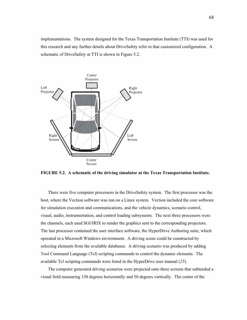
68
implementations. The system designed for the Texas Transportation Institute (TTI) was used for
this research and any further details about DriveSafety refer to that customized configuration. A
schematic of DriveSafety at TTI is shown in Figure 5.2.
FIGURE 5.2. A schematic of the driving simulator at the Texas Transportation Institute.
There were five computer processors in the DriveSafety system. The first processor was the
host, where the Vection software was run on a Linux system. Vection included the core software
for simulation execution and communications, and the vehicle dynamics, scenario control,
visual, audio, instrumentation, and control loading subsystems. The next three processors were
the channels, each used SGI/IRIX to render the graphics sent to the corresponding projectors.
The last processor contained the user interface software, the HyperDrive Authoring suite, which
operated in a Microsoft Windows environment. A driving scene could be constructed by
selecting elements from the available databases. A driving scenario was produced by adding
Tool Command Language (Tcl) scripting commands to control the dynamic elements. The
available Tcl scripting commands were listed in the HyperDrive user manual (25).
The computer generated driving scenarios were projected onto three screens that subtended a
visual field measuring 150 degrees horizontally and 50 degrees vertically. The center of the

69
visual field was located at the driver’s head position, as depicted in Figure 5.2. The images for
the rear view and side mirrors were superimposed onto the forward image. The color images
were high resolution (1024 x 768) textured graphics.
The test vehicle was a full size, 1995 Saturn SL1 and had a full instrumentation package
including speedometer and odometer. The accelerator, brake, and steering wheel were used to
navigate through the driving scenario, interacting with the roadway and vehicles. There was a
force feedback electric servomotor for steering feedback, operating at 800 Hz.
Acceleration performance tests were conducted to illustrate the acceleration capabilities of
the test vehicle. From a stopped position, the accelerator was fully depressed and the speed and
acceleration of the test vehicle were recorded. A sample acceleration curve is shown in Figure
5.3. Reading from this figure, it appears that the acceleration rate increased to 4.0 m/s2, then
dropped down to 3.0 m/s2 at 30 km/h, then to 1.5 m/s2 at 50 km/h, then to 0.8 m/s2 at 95 km/h,
and finally to zero at a maximum speed of 110 km/h. It should be noted that during the initial
acceleration, the maximum acceleration was not achieved. The logic contained within the
Vection software controlled the amount of acceleration to avoid slip between the road and tires.
00.5
11.5
22.5
33.5
44.5
395 400 405 410 415 420
Simulation Time, s
Acc
eler
atio
n (m
/s2 )
0
20
40
60
80
100
120Sp
eed
(km
/h)
Acceleration Speed
FIGURE 5.3. A sample of the acceleration capabilities of DriveSafety.

70
Similar tests were conducted to determine the deceleration capabilities of the test vehicle.
The test vehicle was brought up to a speed of approximately 100 km/h and then the brake pedal
was fully depressed. The speed and deceleration of the test vehicle was recorded. A sample
deceleration curve is shown in Figure 5.4. It appears that the test vehicle had a maximum
deceleration rate of a little over –8 m/s2. Upon the initial and final moments of braking, the
maximum deceleration was not achieved. It is believed that the response of the vehicle was
dampened in the Vection software, thereby limiting the jerk. This also reduced the sudden
vertical shift of the visual display representing the pitch of the test vehicle.
-9-8-7-6-5-4-3-2-10
391 392 393 394 395 396 397 398
Simulation Time, s
Dec
eler
atio
n (m
/s2 )
0
20
40
60
80
100
120
Spee
d (k
m/h
)
Deceleration Speed
FIGURE 5.4. A sample of the deceleration capabilities of DriveSafety.
5.2.3 Model Elements
In order for a VISSIM simulation and a DriveSafety simulation to be integrated into a distributed
simulation, the descriptions of the roadway models needed to be consistent. VISSIM used link-
connector topography to create a model of the roadway network, and allowed the endpoints of
each link and connector to be located at specific x and y coordinates. The number of lanes, lane
widths, gradient, length, direction of traffic, could be defined. Links could also be defined to

71
restrict certain vehicles. This approach was quite flexible and could be used to create a model
that compared to a model created in DriveSafety. For the DriveSafety simulation, the scene was
created using the HyperDrive Authoring suite by selecting existing roadway tiles from a
database. Each tile typically represented 200 x 200 meters of topography including roadway and
elements typical of the culture. A tile could be positioned so that a chosen corner of the tile was
located at any 100 increment of the x and y coordinates. The available cultures included rural,
urban, suburban, residential, industrial, and freeway settings. The availability of two-lane, three-
lane, one-way, two-way, intersections, straight roadway, and curves differed by culture. In each
of these programs, it was possible to develop a model of a straight, two-lane, two-way, rural
roadway needed to address the passing behavior problem.
The vehicles in DriveSafety and VISSIM also needed to be consistent. In DriveSafety, up to
a maximum of 256 vehicles could be included in one scenario, by selecting the different vehicles
from an existing database. Vehicles were classed as emergency, construction, commercial, and
passenger vehicles. All of these vehicles had two axles and the sizes and colors were fixed for
the individual vehicles. For instance, the Grand Prix was 4.72 meters long and 1.556 meters
wide and was available in blue, green, red, tan, and white. The commercial bus was 13.062
meters long and 2.884 meters wide and was only available in white. Any one of these vehicles
could be modeled in VISSIM by defining the vehicle type, class, and category and specifying the
length, width, color, location of axles, and acceleration and deceleration characteristics. By
using two vehicles that differ in length, such as the Grand Prix and the commercial bus, different
passing situations could be programmed such that the lengths of the impeding vehicles differ.
The decision to use a distributed simulation was, in part, based on the differences in how
traffic flows were generated and how vehicles interacted in the different simulations. In
DriveSafety, vehicles were either randomly generated to produce an ambient traffic flow or
individually created using Tcl scripting commands. Each vehicle was created with a default set
of parameter values that prescribed how the vehicles moved and interacted. The parameters
included the desired speed, acceleration, deceleration, headway, and tailway. To produce
variability in vehicle behaviors these parameter values needed to be changed by issuing the
appropriate Tcl scripting commands. The commands could be issued in a start-up file, in a time
procedure that ran at a specific time, in a location trigger activated when a vehicle passed over it,
or in a virtual trigger that activated at a specified rate. Generating a specific traffic flow using
DeriveSafety’s traffic generation mechanisms was very difficult and time consuming, and was

72
much easier using VISSIM. By defining the traffic volumes, traffic composition, speed
distributions, and vehicle acceleration profiles for specific time intervals during the simulation, a
specific and/or calibrated traffic flow could be created in a VISSIM simulation. The vehicles
interacted according to the psychophysical car following logic based on Wiedemann’s (66, 67)
work and the lane changing logic originally designed by Sparmann (76). These models of
driving behavior were stochastic, and therefore introduced variability in the vehicle movements.
5.2.4 Simulation Output
The need for both traffic and behavior data to address the passing behavior problem was the key
motivation for using a distributed simulation. The VISSIM simulation produced disaggregate
data about all of the vehicles in the simulation and the fidelity of the data was limited by the size
of the time step used for the simulation run. VISSIM could use a fixed simulation time step as
small as one tenth of a second. The data was recorded in a vehicle record output, delineated text
format file that had an .fzp extension. The available data was listed in the VISSIM user manual
(24).
The DriveSafety simulation produced disaggregated data about the test vehicle and one other
specified entity (i.e. element). The data collection rate could be specified in the range of one to
60 times per second. This was possible because the simulation had an update rate of 60 times
per second. The data was recorded in a delineated text (.txt) format file. The available data was
listed in the HyperDrive user manual (25). Information about the activation of triggers, the
creation of vehicles, or the processing of external commands was recorded in a log that was
accessible through the HyperDrive Authoring suite and was in a Hyper Text Markup Language
(.html) format file. The information was also saved in a delineated text (.txt) format file on the
host. The user could telnet into the host to retrieve the file.
5.2.5 Import and Export Capabilities
To contribute to the distributed simulation, each individual simulation needed to have data
import and export capabilities. The VISSIM program was chosen because it included an
external driver Application Program Interface (API) that allowed the import and export of data
via a Dynamic Link Library (.dll). The Drivermodel.dll had an entry point called
DriverModelSetValue used to export data from VISSIM and an entry point called
DriverModelGetValue used to import data to VISSIM. A third entry point called
DriverModelExecuteCommand contained four functions that were called by VISSIM.

73
Driver_Command_Init was called during the initialization of the VISSIM program, the
Driver_Command_Create_Driver was called when an external driver vehicle was created in the
simulation, Driver_Command_Move_Driver was called for each time step for the external driver
vehicles, and Driver_Command_Kill_Driver was called when the external driver vehicle moved
out of the road network. During the execution of a simulation, data about any vehicle could be
imported or exported so long as the External Driver Model check box was selected on the
Vehicle Type dialogue box. The available data about the movement of vehicles is listed in
Tables 5.1 and 5.2.
TABLE 5.1. VISSIM Import Data
Data Parameter Description Driver_Data_Veh_Desired_Velocity The desired non directional velocity (i.e. speed)
(m/s) of the vehicle Driver_Data_Veh_Desired_Acceleration The desired acceleration of the vehicle
TABLE 5.2. VISSIM Export Data
Data Parameter Description Driver_Data_Veh_ID A unique identifier for each individual vehicle Driver_Data_Veh _Lane The current lane occupied by the vehicle Driver_Data_Veh _Lane_Angle The current angle (rad) of the vehicle relative to the
middle of the lane Driver_Data_Veh _Lateral_Position The current position (m) of the front of the vehicle to
the middle of the lane Driver_Data_Veh_Velocity The current non directional velocity (i.e. speed) (m/s)
of the vehicle Driver_Data_Veh_Acceleration The current acceleration (m/s2) of the vehicle Driver_Data_Veh_Max_Acceleration Maximum acceleration (m/s2) given current speed Driver_Data_Veh_Desired_Velocity The desired non directional velocity (i.e. speed) (m/s)
of the vehicle Driver_Data_Veh_X_Coordinate The current x-coordinate of the front end of the
vehicle Driver_Data_Veh_Y_Coordinate The current y-coordinate of the front end of the
vehicle
DriveSafety was chosen because communication with external programs was possible
through a socket that used Transmission Control Protocol/Internet Protocol (TCP/IP). TCP
guaranteed that the data was received in the same order that it was sent. A socket program was

74
defined in the initialization script for the DriveSafety simulation, which defined the IP address,
port, and variables needed to put data to and get data from the socket.
Any of the data collection parameters could be exported and any recognized Tcl scripting
commands could be imported. The data collection parameters describing the movement of the
test vehicle (i.e. subject) are listed in Table 5.3. The Tcl scripting commands used to control the
movement of vehicles are listed in Table 5.4.
TABLE 5.3. DriveSafety Export Data
Data Collection Parameter Description LaneName Current lane occupied by subject LanePos Position of the center of the subject in the current lane (m) SubjectHeading Current heading (degrees) with respect to coordinate system Velocity Current non-directional velocity (i.e. speed) (m/s) of the subject X coordinate Current x-coordinate of the center of the test vehicle Y coordinate Current y-coordinate of the center of the test vehicle
TABLE 5.4. DriveSafety Import Data
Tcl Scripting Command Description EntityCreate Creates entity with a unique name with the center located at
the defined x and y coordinates with a zero speed EntityJoinRoadway Joins the named entity to the roadway so the entity can begin
to move EntitySetAcceleration Sets the acceleration behavior of the named entity which is
used when changing the speed of the vehicle EntitySetLanePosition Sets the position of the vehicle in the current lane EntitySetRoadwayVelocity Sets the roadway speed for the named entity EntitySetSpatialState Sets the x and y coordinates of the center of a moving, named
entity
5.3 Step 3: Create the Prototype
The third step in the framework was to create the prototype. The prototype was designed to
allow a test driver in DriveSafety to interact with vehicles controlled by VISSIM by establishing
a two-way, real-time exchange of data between the VISSIM and DriveSafety simulations.
During the development process, delays in the transfer of data were observed and this precluded

75
the two-way real time exchange of data. In the final prototype, the vehicle data from the
VISSIM simulation was transferred to the DriveSafety simulation.
5.3.1 Vehicle Control
The most accurate control of the vehicles would be achieved by updating the x and y coordinate
positions. Unfortunately, using the SetSpatialState scripting command to control the vehicle
positions in DriveSafety caused the vehicles to suddenly stop, change position, and start moving
again. This behavior was not satisfactory. In VISSIM, The x and y coordinate data could not be
imported. Therefore, an alternate approach was required.
The next best approach was to update the velocity of the vehicles. In DriveSafety, vehicle
velocities could be controlled using the EntitySetRoadwayVelocity scripting command. Upon
receiving this command, a vehicle would accelerate or decelerate to the specified speed. The
speed data could also be imported by VISSIM.
The errors in controlling vehicle movements using the velocity data could be explained by
examining the relationship between the velocity data and the x-y coordinate data. If the vehicle
traveled at a constant velocity, the current (instantaneous) velocity data would reflect the change
in the position during the last time step. However, if the average velocity iv , m/s, differed from
the current velocity vi, m/s, then the error in position, m would be equal to:
( tvve iii −= ) (5.1)
where t was the size of the time step, s. With this approach, every time the vehicle changed
velocity, an error in the position of the vehicle would be incurred.
5.3.2 Federation
The design of the federation (i.e. prototype) was based on the HLA standards, and is depicted in
Figure 5.5. The vin attribute referred to the unique identification number of the vehicle and the
type attribute was a description of the vehicle. The xposition attribute referred to the x
coordinate data and the yposition attribute referred to y coordinate data. According to HLA
standards, the exchange of data had to occur through the RTI using implementations of the RTI
services. The RTI could not store data but could convert the format of the data. A translator
program was needed in the DriveSafety federate to translate the vin, type, xposition, and
yposition data to the appropriate Tcl scripting commands.

76
FIGURE 5.5. The design of the HLA-based prototype.
The federation included two simulation federates; the VISSIM federate and the DriveSafety
federate. The federation object model (FOM) described the objects and interactions to be shared
across the federation. The simulation object models (SOMs) for the VISSIM and DriveSafety
federates were identical to the FOM. There was only one object class for this federation, namely
the vehicle object class. It contained the attributes vin, type, xposition, and yposition. The
formats of the vin and type attributes were specified as long and the formats of the xposition and
yposition attributes were specified as double. The object class hierarchy for the federation is
depicted in Figure 5.6 using the Unified Modeling Language graphical notation.
FIGURE 5.6. Depiction of the object classes in the federation.

77
The federation execution data (FED) file contained the FOM information needed for the RTI
to function including the object classes and attributes, and the interaction classes and parameters.
The FED had to include the ObjectRoot class along with the RTIprivate and Manager subclasses,
and the InteractionRoot, and the RTIPrivate and Manager subclasses. For this design, there were
no specified interaction classes.
The RTI initialization data (RID) file contained configuration parameters that controlled the
operation of the RTI software. In this file, network information specific to the execution of this
federation, such as the multicast IP addresses were stored. Both the FED and the RID files
needed to accompany the source files for each federate.
In the final prototype, the vehicle data was transferred from VISSIM to DriveSafety. RTI
data management services were implemented for the RTIambassador and FederateAmbassador
for the VISSIM federate and the DriveSafety federate respectively. These RTI interfaces are
illustrated in Figure 5.7.
FIGURE 5.7. The RTI interfaces in the developed federation
5.3.3 RTI Services
Four RTI data management services were specified for the prototype. Federation management
services were used by the federates to join the federation. Declaration management services
were used by the federates to declare that they would publish and/or subscribe to data during the
simulation execution. Object management services were used to register new instances of an
object class, update the instance attributes, discover new instances, and receive updates of

78
instance attributes. The ownership management services were used to share the instance
attributes by transferring ownership from the VISSIM federate to the DriveSafety federate, and
vice versa.
5.3.4 Advanced RTI Services
The more advanced data distribution management services and the time management services
were not implemented. Because both VISSIM and DriveSafety were proprietary and there was
no access to the interval time advance, the simulations were run independently. Synchronization
of the simulations depended on the efficiency of the data transfers and the ordering of events
relied on the first-in-first-out processing of data across the TCP/IP connections.
5.3.5 VISSIM Federate
The VISSIM federate was comprised of the VISSIM simulation file and the drivermodel.dll that
is used to import/export data using the VISSIM API. The drivermodel.dll was generated in a
Visual C++ environment called drivermodel.dsw. This environment was made up of the
following files:
• Byte_swap.cpp used to convert data to network form before sending to RTI
• FederateAmabassador.cpp contains implementation of federate ambassador services
• Objects.cpp contains the object definitions for RTI services
• DriverModel.cpp contains the external driver routines
• Vissim_interface.cpp has the implementation of the driver_move function
• Rti_interface.cpp contains the implementation of RTI services
• Byte_swap.h contains prototypes for byte_swap.cpp
• FederateAmbassador.h contains prototypes for FederateAmabassador.cpp
• Objects.h contains prototypes for Objects.cpp
• DriverModel.h contains prototypes for the external driver routines
• Vissim_interface.h contains prototypes of the driver_move function
• Rti_interface.h contains prototypes for Rti_interface.cpp

79
Copies of the FED and RID files had to be placed in the same location as the files making up the
drivermodel.dsw environment. To run the VISSIM federate, the drivermodel.dll and copies of
the FED and RID files had to be in the same location as the VISSIM application.
During the development of the VISSIM federate, only one problem was observed. The
output from the API interface did not always compare to the VISSIM data collection file. To
illustrate this problem, the data from the VISSIM data collection file and the API output file are
plotted in Figures 5.8 and 5.9 respectively, for a simulation of a circular roadway network with
one entry point and no exit point that was run for 2000 seconds and had 1073 vehicles enter the
network. During the 28th second, the API did not output any data and the performance of the
API is disturbed between the 469th and 541st seconds. This data could be indicative of a problem
with the API.
0
50
100
150
200
250
300
350
400
0 100 200 300 400 500 600
Time, s
Num
ber o
f veh
icle
upd
ates
pro
cess
ed
FIGURE 5.8. Data output from VISSIM.

80
0
50
100
150
200
250
300
350
400
0 100 200 300 400 500 600
Time, s
Num
ber o
f veh
icle
upd
ates
pro
cess
ed
FIGURE 5.9. Data output from the VISSIM API.
5.3.6 DriveSafety Federate
The DriveSafety federate was comprised of a DriveSafety scenario created using the HyperDrive
Authoring suite and executed in DriveSafety, an interface containing the TCP/IP socket program
to import/export data, and a translator program that used a command generator function to
translate the imported data to Tcl scripting commands. The socket program was located in the
initialization script of the DriveSafety simulation, and defined the IP address, port, and two
string arrays. A polling rate of 60 times per second was specified. The federate was developed
as an executable file that was generated in the VC++ environment called
simulator_interface.dsw. This environment was made up of the following files:
• Byte_swap.cpp used to convert data to network form before sending to RTI
• Simulator_interface.cpp contains the socket program
• Objects.cpp contains the object definitions for RTI services
• Rti_interface.cpp contains the implementation of RTI services
• FederateAmabassador.cpp contains implementation of federate ambassador services
• Command_generator.cpp used to translate instance attributes to Tcl scripting commands

81
• Byte_swap.h contains prototypes for byte_swap.cpp
• Command_generator.h contains prototypes for Command_generator.cpp
• Rti_interface.h contains prototypes for Rti_interface.cpp
• FederateAmbassador.h contains prototypes for FederateAmabassador.cpp
• Objects.h contains prototypes for Objects.cpp
Copies of the FED and RID files had to be placed in the same location as these files making up
the simulator_interface.dsw environment.
During the development of the DriveSafety federate, eight problems were observed. The
first problem was that during any second of the simulation, DriveSafety would process only up
to thirty EntitySetRoadwayVelocity scripting commands received through the socket. As a test,
one thousand EntitySetRoadwayVelocity scripting commands were sent at one time to
DriveSafety. The data from the host log was plotted, as shown in Figure 5.10, revealing that a
maximum of thirty commands were during each second.
0
5
10
15
20
25
30
35
0 5 10 15 20 25
Time, s
Num
ber o
f Ent
itySe
tRoa
dway
Vel
ocity
sc
riptin
g co
mm
ands
pro
cess
ed
FIGURE 5.10. Processing EntitySetRoadwayVelocity commands in DriveSafety
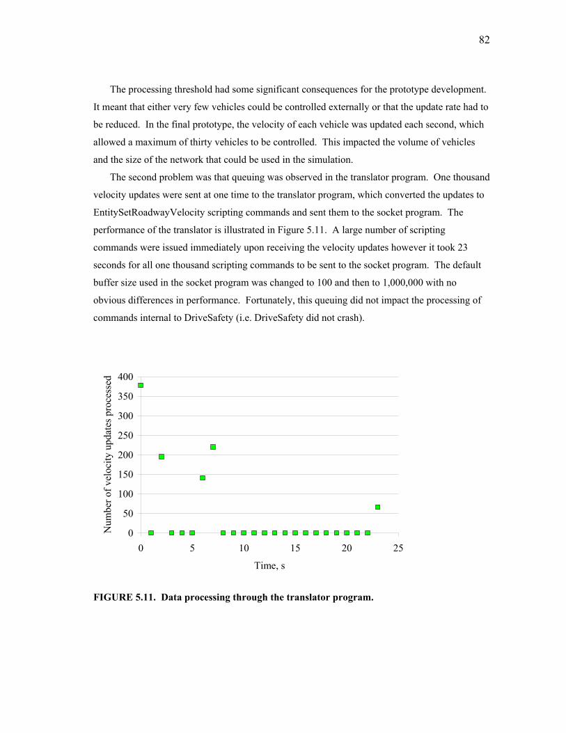
82
The processing threshold had some significant consequences for the prototype development.
It meant that either very few vehicles could be controlled externally or that the update rate had to
be reduced. In the final prototype, the velocity of each vehicle was updated each second, which
allowed a maximum of thirty vehicles to be controlled. This impacted the volume of vehicles
and the size of the network that could be used in the simulation.
The second problem was that queuing was observed in the translator program. One thousand
velocity updates were sent at one time to the translator program, which converted the updates to
EntitySetRoadwayVelocity scripting commands and sent them to the socket program. The
performance of the translator is illustrated in Figure 5.11. A large number of scripting
commands were issued immediately upon receiving the velocity updates however it took 23
seconds for all one thousand scripting commands to be sent to the socket program. The default
buffer size used in the socket program was changed to 100 and then to 1,000,000 with no
obvious differences in performance. Fortunately, this queuing did not impact the processing of
commands internal to DriveSafety (i.e. DriveSafety did not crash).
0
50
100
150
200
250
300
350
400
0 5 10 15 20 25
Time, s
Num
ber o
f vel
ocity
upd
ates
pro
cess
ed
FIGURE 5.11. Data processing through the translator program.

83
The third problem, was that additional queuing was occurring in the translator because the
translator program was written as a single-thread program and could only read or write at one
time. It is hypothesized that a multi-thread translator program and separate sockets for import
and export are needed if a two-way real-time connection is to be established.
The fourth problem was that the socket program used a pulling mechanism to look for new
data from the translator program. The program constantly looked for new data and caused the
computer-processing unit (CPU) to operate at 100% utilization for the duration of the simulation.
This could potentially cause other performance problems. An improvement would be to replace
the pulling mechanism with either a shared memory area, or the use of a dynamic data exchange
technique (120).
The fifth problem was that DriveSafety did not recognize certain vehicle types when used in
externally issued commands. Therefore, data about the vehicle types commercial bus and transit
bus could not be transferred. The FOM, SOMs and name convention used in DriveSafety were
reviewed and no explanation for this phenomenon was found. The vehicle type box truck was
used instead. In DriveSafety, this vehicle is 6.31 meters long and 2.17 meters wide. A similar
vehicle was defined in VISSIM.
The sixth problem was that on occasion, the starting xposition and yposition for a new
vehicle sent from VISSIM to DriveSafety referenced a location outside of the roadway network.
When this occurred, the vehicle failed to join the roadway and subsequent velocity updates for
that vehicle were processed without producing any results. This problem was addressed by the
extended the endpoints of the network in DriveSafety slightly beyond the endpoints of the
network in VISSIM.
The seventh problem was that when the EntitySetRoadwayVelocity commands issued in
DriveSafety required the vehicle to slow down, the brake lights would illuminate. Because the
VISSIM vehicle traveled at a desired speed with some stochastic variation, the brakes lights on
the vehicles in DriveSafety were observed to flash quite often. The solution was to deactivate
the brake lights by issuing the EntitySetBrakeLight scripting command using a location trigger
activated as each vehicle drove over it. An alternate solution would have been to adjust the
tolerance for illuminating the brake lights such that the brake lights would only illuminate under
large decelerations.
The eighth problem was that DriveSafety considered the externally controlled vehicles as
ambient vehicles. This meant that at intersections, and other routing decision points,

84
DriveSafety randomly directed these vehicles, causing vehicles to make unexpected turns. The
solution was to place location triggers that initiated the EntitySelectTurn scripting command
thereby directing vehicles to continue straight through the intersection.
5.3.7 Initialization of the Prototype
To use the federation, comparable simulations were first created in VISSIM and DriveSafety,
meaning they contained the same road network and mapped to the same x and y coordinate
origin. Performing the following four steps initialized the federation:
1. Run the RTI software;
2. Execute the DriveSafety federate (Simulator_interface.exe);
3. Run the DriveSafety simulation;
4. Execute the VISSIM program; and
5. Run the VISSIM simulation.
The federation was created when the DriveSafety federate was executed, and at the same
time, the DriveSafety federate joined the federation. When the DriveSafety simulation was run,
the socket program and translator program were initialized. The VISSIM federate joined the
federation when the VISSIM program was executed. The RTI service to create a federation was
called but the RTI received a message saying it was already created. The drivermodel.dll was
initiated when the VISSIM simulation was run.
5.3.8 Execution of the Prototype
Each time a new vehicle was created in VISSIM, the VISSIM federate registered a new object
instance and updated the attributes of that instance. The instance attributes were reflected in the
FederateAmbassador and the data was sent to the translator program, which used the command
generator function to generate the following Tcl scripting commands
• EntityCreate to create a new vehicle
• EntityJoinRoadway to join the vehicle to the roadway so that it can move
• EntitySetAcceleration to set the acceleration and deceleration behavior of the vehicle

85
For each subsequent instance of the attributes, the average velocity was calculated in the
FederateAmbassador using the xposition and yposition for the current and previous updates, and
was sent along with the instance attributes to the translator. The translator used the command
generator function to generate the EntitySetRoadwayVelocity scripting commands. They were
stored in a global string array, which had a bottom-in and top-out queuing. The socket program
read the Tcl scripting commands and passed them to DriveSafety over a TCP/IP socket.
The execution of the final prototype produced a driving environment that was visually
comparable to the driving environments produced using DriveSafety as a stand-alone simulation.
The simulation progressed without any noticeable discontinuities in the time advance. The
creation of vehicles and the velocities were prescribed by the data from VISSIM however
DriveSafety still maintained primary control of the vehicles. The advantage of using the
prototype was that a specific traffic flow could be created. The test driver could interact with the
vehicles even though a two-way real-time exchange of data was not achieved. The driver data
could be collected using DriveSafety, and the traffic data could be collected using VISSIM,
although the traffic data would only be an estimation of the vehicle movements observed by the
test driver.
5.3.9 Communication Within the Final Prototype
In this section, the communication within the federation is examined by comparing the output
files from the VISSIM simulation, the drivermodel.dll interface, the translator program, and
DriveSafety simulation. The file formats are indicated on Figure 5.12. The html and fzp files
were converted into a text format file and all the text format files were imported into Excel
spreadsheets.
FIGURE 5.12. The data files that were available to evaluate the federation.

86
Comparing the output was complicated by the fact that the VISSIM simulation and the
DriveSafety simulation referenced different time clocks than the drivermodel.dll and the
translator program as depicted in Figure 5.12. The VISSIM simulation referenced the simulation
time, which was the logical time, used to advance the simulation. The drivermodel.dll and the
translator program referenced the time of the first computer-processing unit (CPU), labeled
CPU1. The DriveSafety simulation output referenced the time of the second CPU, labeled CPU2
The federation was executed and the VISSIM.fzp, API.txt, Translator.txt, and
DriveSafety.html files were examined. In each file, the time was recorded to the nearest second.
The referenced time and the first five times recorded in each file are shown in Figure 5.13. The
size of the time offsets, labeled O1 and O2 were unknown. It was assumed that the absolute
value of the time offset was not greater than one second, which meant that the delay in
transferring data between VISSIM and the API, and between the translator and VISSIM was
assumed to be less than one second. The files were aligned according to the logical processing
of the data being transferred from VISSIM to DriveSafety.
FIGURE 5.13. A depiction of the comparing the time in the output files.

87
To demonstrate the process of aligning the files, the first data transfer (the creation of the
first vehicle) was tracked in each of the files, as indicated by the arrows in Figure 5.13. In the
VISSIM.fzp file the data was recorded at time 2, in the API.txt file it was recorded at 16:57:36,
in the Translator.txt file it was recorded at 16:57:37, and in the DriveSafety.html file it was
recorded at 15:37:51. Because the time was recorded to the nearest second, the arrows could
have been drawn anywhere within the individual time intervals. A vertical solid arrow
represents a data transfer that had no time delay and a dotted arrow represents a data transfer that
was delayed. This was repeated for each subsequent data transfer to ensure that the alignment of
the files reflects the logical processing order.
5.3.9.1 Queuing. Queuing occurred in both the VISSIM federate and the DriveSafety federate,
as previously discussed in sections 5.3.5.and 5.3.6 respectively. The queuing is apparent when
comparing the number of vehicle instances (i.e. updates) processed by the VISSIM simulation,
the API interface, the translator program, and the DriveSafety simulation, during a run of the
prototype, as shown in Figures 5.14 though 5.17 respectively. The time used on the x-axis refers
to the amount of time that passed since the transfer of the data for the first vehicle created.
05
101520253035404550
0 50 100 150 200 250 300 350 400 450
Time, s
Num
ber o
f Veh
icle
Inst
ance
s
FIGURE 5.14. Number of vehicle instances recorded in the VISSIM.fzp file.

88
05
101520253035404550
0 50 100 150 200 250 300 350 400 450
Time, s
Num
ber o
f Veh
icle
Inst
ance
s
FIGURE 5.15. Number of vehicle instances recorded in the API.txt file.
05
101520253035404550
0 50 100 150 200 250 300 350 400 450
Time, s
Num
ber o
f Veh
icle
Inst
ance
s
FIGURE 5.16. Number of vehicle instances recorded in the Tranlstor.txt file.

89
05
101520253035404550
0 50 100 150 200 250 300 350 400 450
Time, s
Num
ber o
f Veh
icle
Inst
ance
s
FIGURE 5.17. Number of vehicle instances recorded in the DriveSafety.html file.
If queuing had not occurred during the simulation run, the plots in Figures 5.14 through 5.17
would be identical. Therefore, any difference between any two consecutive plots is evidence of
queuing. It appears that queuing occurred between VISSIM and the API, between the API and
the translator, and between the translator and DriveSafety.
5.3.10 Vehicle Position Error
Errors in vehicle positions were expected because the speed data was used to control the vehicle
movements, as discussed in section 5.3.1. The vehicle position error is the difference between
the expected location (xe) of the vehicle, as given by the VISSIM simulation, and the actual
location (xa) observed in the DriveSafety simulation. It can be described as the integral of the
differences between the speeds of the vehicles over the time interval from zero to t, and can be
estimated by:
∑
−
t
0ae
∆t∆x
∆t∆x
(5.3)

90
There were several reasons why the vehicles in DriveSafety deviated from their expected
positions. The first reason was the difference in how vehicles were created. VISSIM vehicles
entered the network with a speed whereas in DriveSafety vehicles were created with zero speed
and joined the network from a stopped position. The second reason was the time delay that
occurred while transferring vehicle instances from VISSIM to DriveSafety. The third reason
was that the acceleration behavior of the vehicles in VISSIM and DriveSafety differed and
would cause vehicle position errors during speed changes. The fourth reason was that the
vehicles in DriveSafety might have reacted to the test vehicle thereby causing speed changes.
To illustrate the position error, the VISSIM.fzp file and the DriveSafety.html file were
collected for a single simulation run and the speed outputs were compared. Starting at the
VISSIM simulation time 288 seconds, the vehicle position errors for the first vehicle created
were calculated as the difference in the x positions in the two files. In Figure 5.28, the vehicle
position error is shown with respect to the VISSIM simulation time. A negative vehicle position
error indicates that the DriveSafety vehicle was trailing behind the expected position. The speed
of the vehicle is also shown. It is seen in Figure 5.18, that when the speed increased the vehicle
lagged further behind the expected position.
-40
-35
-30
-25
-20
-15
-10
-5
0288 293 298 303 308
VISSIM Simulation Time, s
Veh
icle
Pos
ition
Err
or, m
0
5
10
15
20
25
Veh
icle
Spe
ed, m
/sVehicle Position Error Vehicle Speed
FIGURE 5.18. The vehicle position error.

91
5.4 Recommendations
Based on the problems encountered during the creation of the prototype, several
recommendations were made. Addressing these recommendations would pave the way for a
future two-way real time exchange of data in the prototype.
5.4.1 VISSIM
The sporadic queuing of data between the VISSIM simulation and the API needs to be
examined. If the queuing stemmed from how the API was programmed, then changes are
needed to ensure that the API exports data during every time step. Without this correction, there
will be difficulties incorporating a VISSIM simulation into a distributed simulation designed for
two-way real-time data exchange. It is also possible that the queuing was the result of poor CPU
memory management, in which case, that issue would need to be addressed.
5.4.2 DriveSafety
In DriveSafety, vehicles were created with zero speed. A request was submitted to the
developers to allow vehicles to be created with a non-zero speed. This request was addressed
and the EntityCreate command was changed to include a speed parameter.
During the development of the prototype, a processing threshold of thirty EntitySetVelocity
scripting commands was identified. Although 254 vehicles could be included in the simulation,
only thirty could be controlled externally. This threshold limited the update rate, the number of
vehicles in the simulation, and therefore the traffic flow and network size. To increase the
usefulness of DriveSafety, and make it more desirable for distributed simulations, this threshold
need to be increased.
The socket program used an indefinite loop to pull data, which is the least desirable method
to get new data from an external source. The operation of the socket needs to be re-evaluated.
The used of a shared memory or dynamic data exchange techniques would be preferable.
5.4.3 Translator Program
The translator program was developed to translate the text format information from the VISSIM
API into Tcl scripting commands read by DriveSafety. This program was developed in C++ as a
single thread program. To allow data to be read and written simultaneously, the program needs
to be developed as a multithread program and run in a Windows type environment.

92
5.4.4 Prototype
The prototype included simulations creating using two proprietary programs. Each has its own
internal clock to control the advance of the individual simulations. In a distributed simulation,
where the data is transferred in real-time between the individual simulations, the HLA time
management tools really need to be implemented to synchronize the simulations. Because of the
proprietary nature of the programs this was not possible. It is recommended that in the future,
greater consideration of the access to the source code and the ability to manipulate the time
advance should be given when selecting the contributing simulations.

93
6 APPLICATION OF THE PROTOTYPE*
This passing application is only one example of how the methodology could be applied. Other
prototype distributed traffic simulations could be created and used to study other specific traffic
and/or behavior problems. The details of this passing experiment were submitted to the
Institutional Review Board at the Texas A&M University. Approval was granted based on the
experimental design, selection of test drivers, risk to the test drivers, and the experimental
procedures described in the following sections. Copies of the approval letters are located in
Appendix D.
6.1 Experimental Design
The experiment had a 2x2 factorial design with repeated measures on both factors, where both
the type of impeding vehicle (car or truck) and the speed of the impeding vehicle (fast or slow)
were fixed effects factors. The dependent factors were the time and distance traveled in the left
lane during the passing maneuver. The experiment was designed to have test drivers follow an
impeding vehicle on a simulated two-lane rural road and then accelerate and pass. The test
drivers had to choose to accept a gap in the opposing traffic to complete the maneuver.
6.2 Test Drivers
Thirty test drivers, sixteen females and fourteen males, were recruited from Texas A&M
University and the community through person-to-person contact. To avoid including drivers
with little driving experience, which are generally over represented in vehicle accident statistics
(170), each test driver had at least 5 years of driving experience. Six of these test drivers were
replacements for those who either did not complete the study or failed to make the desired
passing maneuvers. In the end, the data for twelve male and twelve female test drivers, ranging
in age from 23 to 57 years was collected. The four passing conditions could be ordered in 24
*Reprinted with permission from Jenkins, J., and L. R. Rilett. Application of a Distributed Traffic Simulation for a Passing Behavior Study. Presented at Transportation Research Board 83rd Annual Meeting, Washington, D. C., 2004. (Accepted for publication in Transportation Research Record: Journal of the Transportation Research Board, TRB, National Research Council, Washington, D.C., 2004 [in preparation]).

94
unique combinations. The ordering combinations were randomly assigned to the 24 test drivers
to control for any ordering effects. The final schedule is located in Appendix E.
6.2.1 Risks
The test drivers were told that they may experience symptoms of simulator sickness, including
eyestrain, headache, dizziness, and nausea. Only one of the thirty test drivers chose not to
complete the experiment because of some discomfort. The remaining twenty-nine test drivers
completed the experiment. All test drivers completed the simulator sickness questionnaire found
in Appendix F and reported the severity of the simulator sickness symptoms experienced during
the study. Their responses are listed in Appendix G and summarized in Table 6.1.
TABLE 6.1. Reported Severity of Simulator Sickness Symptoms
Reported severity Symptom Experienced None Low Moderate High Eye Strain 13 15 2 0 Headache 22 7 1 0 Dizziness 16 12 1 1 Nausea 22 6 1 1
6.3 Experimental Procedure
After reading and signing a copy of the consent form found in Appendix H, each test driver
drove the practice scenario once and the experimental scenario four times.
6.3.1 Practice Scenario
The practice scenario, developed using DriveSafety as a stand-alone simulation, was to acclimate
the test drivers to the simulated driving environment. A schematic of the practice scenario is
shown in Figure 6.1. For the practice scenario, test drivers were instructed to follow the lead
vehicle. As the test vehicle began to move the lead vehicle advanced and continued down the
two-lane road through an industrial area at 72 km/h (45 mph) and a rural area at 88 km/h (55
mph). The instructions are included in Appendix I. The roadway was approximately 5 km long
and took approximately 4 minutes to drive. The scenario ended when the test driver arrived at a
stop controlled t-intersection and was instructed to place the vehicle transmission in park. All

95
test drivers were observed to have good control of the simulated vehicle. Data was not collected
to confirm this observation.
FIGURE 6.1. Schematic of the practice scenario with a sample center screen image.
6.3.2 Experimental Scenario
The experimental scenario was developed using the prototype distributed traffic simulation. The
VISSIM simulation controlled the creation and the speed of all vehicles excluding the test
vehicle. A schematic of the experimental scenario is shown in Figure 6.2. The scenario had
over 10 km of roadway, including 4 km of road through an industrial area and 4 km of road
through a rural area. The posted speed limits were 72 km/h (45 mph) in the industrial area and
88 km/h (55 mph) in the rural area. The scenario took approximately 7 minutes to drive.

96
FIGURE 6.2. Schematic of the experimental scenario with sample center screen images.
As shown in Figure 6.3, two separate platoons, each with a lead car, truck, and second car,
entered the network at the beginning of the simulation and traveled in the center of the test
vehicle’s lane. The impeding vehicles traveled at speeds less than the posted speed limit to
create a passing situation. The first and second platoons were respectively programmed to travel
approximately 8 km/h (5 mph) and 16 km/h (10 mph) below the speed limit. The lead car and
the truck in each platoon were the impeding vehicles to be passed. The cars were 4.72 m long

97
and the trucks were 6.31 m long. These were the lengths of the vehicles in DriveSafety and were
mimicked in VISSIM.
FIGURE 6.3. Illustration of the two platoons of impeding vehicles.
To ensure that the test driver did not see vehicles magically appear and begin to drive along
the roadway, it was necessary to populate the scenario from the end points of the roadway. The
opposing traffic entered at a volume of 250 vehicles per hour and traveled at approximately the
speed limit. The VISSIM simulation also controlled the volumes and speeds of these vehicles
and the flow of opposing vehicles began at the beginning of the simulation. The industrial and
rural roadway sections were sized so that the drivers would have opposing traffic when they
entered the rural passing area. This was necessary to ensure that the passing did not take place at
the beginning of the passing area where the speed limit changed from 45 mph to 55 mph.
The simulated environment posed a constraint on the available sight distance. Objects
appeared 500 meters ahead of the test vehicle on the apparent horizon. When the opposing
vehicle was 500 m or more upstream, there was ample distance for the test driver to successfully
complete the passing maneuver. At higher speeds, this constraint could have limited the passing
opportunity.
At the beginning of each experimental scenario, test drivers were stopped at the location
labeled “Start” in Figure 6.2. They were instructed to turn right onto the roadway behind a
particular vehicle in one of the two platoons that would approach from their left. Test drivers
were instructed to pass the slower impeding vehicles in a safe and judicious manner, pass only in
the rural passing area, and pass only one vehicle at a time. To complete a passing maneuver, the
driver had to choose an acceptable gap in the opposing traffic. After driving through the rural
area, the test drivers were instructed to pull over onto the shoulder and place the vehicle
transmission in park. The instructions for the experimental scenario are included in Appendix I.

98
6.4 Data Collection
If a two-way, real-time communication had been established in the prototype, the position and
speed of every vehicle would have been available directly from the VISSIM simulation output.
However, the prototype operated with a one-way communication that experienced time delays in
the transfer of vehicle data from VISSIM to DriveSafety. Therefore, two methods were used to
collect the data, one for the impeding and passing vehicles and a second for the opposing
vehicles.
6.4.1 Impeding and Passing Vehicle Data
DriveSafety had tools to collect data about the test vehicle and one named entity, in this case the
impeding vehicle. These tools were use to record the time, x-y coordinate of the center of the
vehicle, heading, speed, and acceleration data of the test vehicle, the gap between the impeding
and passing vehicle, the linear distance between the centers of the impeding and passing
vehicles, and the speed of the impeding vehicle, all at a rate of ten times per second. The
quantity and quality of this data far exceeded what has been captured in the field using
traditional techniques. It was possible to record the data at 60 times per second but the
additional time and effort to reduce six times the amount of data did not warrant the small
differences that could be obtained. Using a location trigger placed at the beginning of the rural
area, the name of the impeding vehicle was queried so that it could be included in the data
collection file. The location trigger also activated the recording of the data. A second location
trigger placed at the end of the rural area deactivated the recording of data.
6.4.2 Opposing Vehicle Data
Data about the opposing vehicles in the experimental scenario was not available through the
DriveSafety data collection tools. Instead, the vehicle locations were estimated by analyzing the
activity of location triggers placed along the rural passing area that were activated every time a
vehicle drove over them. The locations triggers were placed at the coordinate locations
(4500,700), (5500, 700), (6500, 700), (7500,700) and (8500, 700) as identified in Figure 6.4.

99
FIGURE 6.4. Coordinates of the location triggers.
The location trigger activation data was recorded in the host log of DriveSafety. Because the
simulation was the same for each experimental scenario run, the data for the opposing vehicles
was only reduced once. The vehicle trajectories of the opposing vehicles and the impeding
vehicles are shown in Figure 6.5. These trajectories estimated the location of the center of the
vehicles because the triggers were activated when the center of the vehicle crossed over the edge
of the location trigger.
45004750500052505500575060006250650067507000725075007750800082508500
300
310
320
330
340
350
360
370
380
390
400
410
420
430
440
450
460
470
480
490
500
Simulation Time, s
X C
oord
inat
e, m
FIGURE 6.5. Estimated trajectories of the opposing vehicle using location trigger data.

100
Also using the data about the activation of the location triggers, a set of linear regression
equations was developed to describe the estimated trajectories of each of the opposing vehicles.
These equations are shown in Table 6.2.
These trajectory equations referenced the simulation time, t, of one particular simulation run.
However, this time varied between experimental scenario runs so a method was needed to link
these trajectories to the movement of the opposing vehicles during each passing maneuver.
Because VISSIM controlled both the opposing and the impeding vehicles, the movements of the
impeding vehicles observed during each simulation run could be used to align the simulation
time of each experimental scenario run with the simulation time referenced in the trajectory
equations. To do this the trajectory equations for the impeding vehicles were needed. These are
shown in Table 6.3
TABLE 6.2. Linear Regression Equations of Opposing Vehicle Trajectories
Vehicle ID Vehicle Description Estimated Trajectory v10 Purple Celica xo = -24.271t + 11569 v11 Purple Celica xo = -23.923t + 11687 v12 Purple Celica xo = -23.98t + 11762 v13 Blue Lexus xo = -24.154t + 12226 v14 Purple Celica xo = -24.096t + 12265 v15 White Grand Prix xo = -24.39t + 12940 v16 Blue Lexus xo = -24.213t + 13368 v17 Purple Celica xo = -24.213t + 13561 v18 Gray Lexus xo = -24.213t + 13513 v19 Gray Lexus xo = -23.98t + 14909 v20 Blue Lexus xo = -24.271t + 15374 v21 Blue Lexus xo = -23.923t + 15898 v22 White Grand Prix xo = -23.923t + 15946 v23 Purple Celica xo = -24.154t + 16283 v24 Gray Lexus xo = -24.096t + 16337 v25 Purple Celica xo = -23.98t + 16343 v26 Purple Celica xo = -24.213t + 16830 v27 Blue Lexus xo = -24.154t + 16863 v28 Blue Lexus xo = -24.213t + 17532 v29 Purple Celica xo = -23.98t + 18553 v30 White Grand Prix xo = -24.038t + 18647 v31 Purple Celica xo = -24.095t + 19276 v32 White Grand Prix xo = -24.095t + 19444

101
TABLE 6.3. Linear Regression Equations of Impeding Vehicle Trajectories
Vehicle ID Vehicle Description Estimated Trajectories v1 Red Grand Prix xi = 21.459t - 1548.1 v2 White Box Truck xi = 21.551t - 1647.4 v3 Red Grand Prix xi = 21.551t - 1755.2 v5 Blue Grand Prix xi = 19.342t - 1210.8 v7 Gray Box Truck xi = 19.493t - 1387.8 v8 Blue Grand Prix xi = 19.342t - 1442.9
TABLE 6.4. Vehicle Lengths and Widths
Vehicle ID Vehicle Description Length To Back, m Length To Front, m Width ,m Test Vehicle Beige Saturn 2.3595 2.3595 1.556
v1 Red Grand Prix 2.359 2.359 1.556 v2 White Box Truck 3.499 2.811 2.17 v3 Red Grand Prix 2.359 2.359 1.556 v5 Blue Grand Prix 2.359 2.359 1.556 v7 Gray Box Truck 3.499 2.811 2.17 v8 Blue Grand Prix 2.359 2.359 1.556
v10 Purple Celica 1.887 2.156 1.728 v11 Purple Celica 1.887 2.156 1.728 v12 Purple Celica 1.887 2.156 1.728 v13 Blue Lexus 2.405 2.405 1.762 v14 Purple Celica 1.887 2.156 1.728 v15 White Grand Prix 2.359 2.359 1.556 v16 Blue Lexus 2.405 2.405 1.762 v17 Purple Celica 1.887 2.156 1.728 v18 Gray Lexus 2.405 2.405 1.762 v19 Gray Lexus 2.405 2.405 1.762 v20 Blue Lexus 2.405 2.405 1.762 v21 Blue Lexus 2.405 2.405 1.762 v22 White Grand Prix 2.359 2.359 1.556 v23 Purple Celica 1.887 2.156 1.728 v24 Gray Lexus 2.405 2.405 1.762 v25 Purple Celica 1.887 2.156 1.728 v26 Purple Celica 1.887 2.156 1.728 v27 Blue Lexus 2.405 2.405 1.762 v28 Blue Lexus 2.405 2.405 1.762 v29 Purple Celica 1.887 2.156 1.728 v30 White Grand Prix 2.359 2.359 1.556 v31 Purple Celica 1.887 2.156 1.728 v32 White Grand Prix 2.359 2.359 1.556

102
The position of the center of the impeding vehicle xi given in the output was used with the
appropriate estimated trajectory equation from Table 6.3 to calculate the simulation reference
time, t. That time was then used with the appropriate estimated trajectory equations for the
opposing vehicles from Table 6.2 to calculate the location of the center of the opposing vehicles,
xo.
The positions of the impeding and opposing vehicles, and their corresponding trajectory
equations, referenced the center of the vehicle. To determine the gaps between opposing
vehicles, the lengths of the opposing vehicles were needed. The lengths and widths for all the
impeding and opposing vehicles are given in Table 6.4. Gaps between opposing vehicles were
found to range from roughly 20 to 1450 m.
For each test driver, the data was put into an Excel workbook, each containing one
worksheet for each experimental scenario run. A typical worksheet was twenty columns by
approximately one thousand rows. Capturing similar data in the field would be very difficult.
Even if photographic techniques could be implored to capture the movement of every vehicle,
the data reduction efforts would be enormous.
6.4.3 Surveys, Questionnaires and Interviews
In addition to the electronically recorded data, detailed information about the test drivers could
have been elicited through surveys, questionnaires, or personal interviews. Experiments such as
this one, which used a simulated environment conducted in a laboratory setting, brings the
researcher or experimenter face-to-face with the test drivers. Comparable interaction is not
available during field studies.
6.4.4 Observations
Apart from the formal interaction between the test driver and the experimenter, the laboratory
setting allowed the experimenter to gain information about the test driver through general
observations. To make observations during a field study, the experimenter would need to be in
close proximity to the test driver. To capture how the behavior changes or to observe the test
driver for a period of time would mean that the experimenter would need to be in the same
vehicle as the test driver, in a neighboring vehicle, or use some technology that has tracking
capabilities, such as Global Positioning Satellite (GPS).
During the passing behavior study, several general observations were recorded. First of all,
all of the test drivers were observed to have good control of the test vehicle. Some difficulties

103
were observed making the right turn onto the industrial roadway from the start position but this
did not impact the experiment. If difficulties were observed during the first experimental
scenario, the test driver was given further verbal instructions on how to better negotiate the turn.
Some drivers complained of some discomfort when braking at the end of the scenarios. If this
was the case, the test driver was further instructed to coast to a stop to reduce their discomfort.
Second, most drivers followed the given instructions. Only one test driver failed to make a
pass during an experimental drive. The data for this test driver was excluded from the analysis.
Three test drivers completed passes where more than one vehicle was passed during a single
maneuver. The data for these test drivers was also excluded from the analysis.
Third, a couple of behaviors were observed that support the notion that the test drivers were
engrossed in the simulated driving environment. These behaviors included the tilting of the head
to the left to see around the impeding vehicle, the sampling of the rear view image, and avoiding
collisions. Given that the animation was presented in two dimensions, any shifting of the head
did not change what was viewed. Therefore, it was interesting to see test drivers repeatedly
tilted their heads to get a better look at whether there was opposing traffic present. Test drivers
were also observed looking at the rear view, which was integrated in the center forward view. It
appeared that drivers looked at this image when returning to the right lane. For the most part,
test drivers avoided collisions with the impeding and the opposing vehicles. In six passing
maneuvers, the driver decided to abort the maneuver and return to the right lane behind the
original impeding vehicle. In each case, a passing maneuver was successfully completed further
downstream. Only in one passing maneuver for one test driver did a collision with an opposing
vehicle occur. This test driver had a lot of previous experience driving in simulated
environments and admitted that there is no longer any perceived risk when driving. The data for
this test driver was excluded from the analysis.
6.5 Data Reduction – Conventional Definition
The data from the experimental scenario under each of the four passing conditions for all of the
24 test drivers was examined. Each passing maneuver was labeled using the test driver number
followed by the sex of the test driver and the trial number. For instance, the four passing
maneuvers performed by the first test driver, who was male, would be identified by 1M1, 1M2,
1M3, and 1M4.

104
For each passing maneuver, the time and distance in the left lane, start gap distance, and end
gap distance were calculated. The time (t2) and distance (d2) that the passing vehicle occupied
the left lane was defined as:
beginning when the front left wheel crossed over the centerline as the passing vehicle moved
into the left lane; and
•
• ending when the rear left wheel crossed over the centerline as the passing vehicle moved
back into the right lane.
These are the conventional definitions, and are comparable to that given by AASHTO (10) and
used in previous studies (22, 155). The start gap (GS) was the distance from the front of the
passing vehicle to the rear of the impeding vehicle when the passing vehicle began to occupy the
left lane. It was calculated from the positions of the impeding (xi) and passing (xp) vehicles,
taking into account of the vehicle lengths (Li and Lp) such that:
+−
−=
2L
x2L
xG pp
iiS (6.1)
The end gap (GE) was the distance from the rear of the passing vehicle to the front of the
impeding vehicle when the passing vehicle ceased to occupy the left lane. It was also calculated
from the positions of the impeding (xi) and passing (xp) vehicles, taking into account the vehicle
lengths (Li and Lp) such that:
+−
−=
2L
x2
LxG i
ip
pE (6.2)
The lengths of the passing vehicle and each of the impeding vehicles were previously given in
Table 6.4. Because of the fidelity of the data recorded, other definitions for the time and
distance in the left lane, and gap distances could be used and easily quantified.
A cursory examination revealed that five test drivers performed at least one pass, where the
test vehicle was partially in the left lane while the test driver waited for an acceptable gap in the
oncoming traffic. Six test drivers performed at least one pass where the test vehicle remained in
the left lane at the end of the pass until after the oncoming vehicle passed. These behaviors are

105
inappropriate and could be regarded as potential collisions. The cause of these behaviors was
not explored analytically but it was hypothesized that it could stem from how test drivers judged
their lateral position on the simulated road or perceived the risk of a collision. Three test drivers
exhibited both of these behaviors. The data for 8 test drivers that exhibited either behavior was
excluded, leaving a total of 64 passing maneuvers for analysis. The time and distance in the left
lane, start gap distance, and end gap distance for each of the 64 passing maneuvers is shown in
Appendix J along with a description of the impeding vehicle.
6.5.1 Data Exploration
In preparation for the analysis of the passing data, the distributions of the response variables
were tested using the Kolmogorov-Smirnov (K-S) test for normality. The results are shown in
Table 6.5. At a 0.05 level of significance, the normal distribution was not a good fit for the time
or distance in the left lane for this sample of passing maneuvers. To further explore these
distributions, histograms of the response variable were plotted. The plots are shown in Figure
6.6 and 6.7.
TABLE 6.5. Normality Test Results for Time, Distance, and Gap Distances, N=64
Response Variable
n Mean σ Absolute Extreme Difference
K-S test statistic
Significance
t2 (sec) 64 20.05 10.76 0.202 1.617 0.011 d2 (m) 64 490.30 237.64 0.202 1.613 0.011 GS (m) 64 23.49 12.19 0.155 1.242 0.092 GE (m) 64 47.37 19.25 0.137 1.099 0.178
Note: n is the sample size and σ is the standard deviation.
From the histograms, it is seen that there may be extreme outliers in the time interval labeled
by 70 seconds and the distance interval labeled by 1600 meters. Both of these outliers are from
passing maneuver 7F1. By removing this outlier from the data, the results of the Kolmogorov-
Smirnov (K-S) test for normality at the 0.05 level of significance support that the normal
distribution was a good fit for each of the response variables for this sample of 63 passing
maneuvers. The results are shown in Table 6.6.

106
Time, s
70656055504540353025201510
Freq
uenc
y
20
10
0
FIGURE 6.6. Histogram of the response variable, time in the left lane.
Distance, m
1600
1500
1400
1300
1200
1100
1000900
800
700
600
500
400
300
200
Freq
uenc
y
20
10
0
FIGURE 6.7. Histogram of the response variable, distance in the left lane.

107
TABLE 6.6. Normality Test Results for Time, Distance, and Gap Distances, N=63
Response Variable
n Mean σ Absolute Extreme Difference
K-S test statistic
Significance
t2 (sec) 63 19.23 8.63 0.152 1.206 0.109 d2 (m) 63 472.28 190.43 0.153 1.216 0.104 GS (m) 63 23.45 12.29 0.162 1.283 0.074 GE (m) 63 47.31 19.40 0.146 1.161 0.135
Note: n is the sample size and σ is the standard deviation.
TABLE 6.7. Time, Distance, and Gap Distances – Conventional Definition
Slow Speed Fast Speed All Speeds Response Variable
Impeding Vehicle n Mean σ n Mean σ n Mean σ car 16 17.63 11.43 16 17.38 7.15 32 17.50 9.40 truck 16 19.21 5.58 15 22.94 8.95 31 21.02 7.52 t2 (sec) all 32 18.42 8.89 31 20.07 8.42 63 19.23 8.63 car 16 424.4 241.0 16 449.5 168.4 32 436.9 204.9 truck 16 456.9 123.9 15 563.9 197.5 31 508.7 169.8 d2 (m) all 32 440.6 189.2 31 504.9 189.1 63 472.2 190.4 car 16 22.07 13.26 16 19.58 8.05 32 20.82 10.86 truck 16 24.40 11.02 15 28.05 15.42 31 26.16 13.23 GS (m) all 32 23.23 12.05 31 23.68 12.72 63 23.45 12.29 car 16 53.31 21.45 16 49.28 20.17 32 51.29 20.58 truck 16 49.17 20.68 15 36.82 10.60 31 43.20 17.48 GE (m) All 32 51.24 20.83 31 43.25 17.20 63 47.31 19.40
Note: n is the sample size and σ is the standard deviation.
6.5.2 Data Summary
For the 63 data samples, the averages and standard deviations of the times and distances in the
left lane, start gap distances, and end gap distances are presented in Table 6.7. As expected, it
appears that the time and distance in the left lane, and the start gap distance were greater when
the impeding vehicle was a truck as opposed to a car or when the impeding vehicle was traveling
at the faster of the two speeds. Contrary to expectation, it appears that the end gap distances
were smaller when the impeding vehicle was a truck as opposed to a car or when the impeding
vehicle was traveling at the faster of the two speeds. The data is analyzed in the following
sections.

108
6.6 Data Analysis – Conventional Definition
The first step in the analysis was to examine the factor effects plots for each of the response
variables: the times and distances in the left lane, and the start gap and end gap distances. These
plots illustrate the interaction and the main effects of the two factors: the speed and the length of
the impeding vehicle. The second step in the analysis was to test whether the observed
interaction of the factor effects are significant from a statistical perspective. This test was
carried out using a factor effects analysis of variance (ANOVA) model for two factor
experiments with repeated measures on both factors and assumed that the response variables
were normally distributed. The third step in the analysis was to determine whether the main
effects of the factors were significant by using the same ANOVA model.
6.6.1 Factor Effects Plots
A factor effects plot was used to compare the mean responses given the various levels of the
experiment test factors. The effects of two factors interact if the difference in the mean response
for two levels of one factor is not constant across the levels of the second factor. Visually, this
means that if the lines are parallel, then there is no interaction of factor effects. If the lines are
not parallel, the factor effects do interact and the importance of that interaction is tested using an
F-test. The main effects of the factors are also illustrated in a factor effects plot. For a two-
factor effects plot, the main effect of the first factor is illustrated by the slopes of the lines for
each level of the second factor. The main effect of the second factor is illustrated by the
difference between the lines at each level of the first factors. The factor effect plots for the times
and distances in the left lane and the start gap and end gap distance are shown in Figures 6.8
through 6.11.

109
Length, m
6.314.72
Mea
n Ti
me,
s
24
23
22
21
20
19
18
17
Speed
fast
slow
FIGURE 6.8. Factor effects plot for time in the left lane.
Length, m
6.314.72
Mea
n D
ista
nce,
m
580
560
540
520
500
480
460
440
420400
Speed
fast
slow
FIGURE 6.9. Factor effects plot for distance in the left lane.

110
Length, m
6.314.72
Mea
n St
art G
ap, m
30
28
26
24
22
20
18
Speed
fast
slow
FIGURE 6.10. Factor effects plot for start gap distance.
Length, m
6.314.72
Mea
n En
d G
ap, m
60
50
40
30
Speed
fast
slow
FIGURE 6.11. Factor effects plot for end gap distance.

111
In each of the four factor effects plots, the lines are not parallel, suggesting that the factor
effects interacted. Based on the slopes of the lines and the differences between the lines at the
factor levels, there appears to have been main effects of both factors for all of the response
variables. These relationships were further explored by conducting F-tests for the strengths of
the interaction between the factor effects as well as the main factor effects.
6.6.2 Analysis of Variance Model
The ANOVA model for two factor experiments with repeated measures on both factors,
assuming no interaction between the treatments and the subjects, has the general form:
( ) ijkjkkjiijk εαββαρµY +++++= (6.3)
where is the observation for the iijkY th subject, jth level of factor A and the kth level of factor B;
µ is the overall mean
iρ is the effect due to the ith subject;
jα is the effect due to the jth level of A;
kβ is the effect due to the kth level of B;
( ) jkαβ is the effect due to the jth level of A and the kth level of B; and
ijkε is the random error.
The corresponding ANOVA table is shown in Table 6.8.
TABLE 6.8. ANOVA Table for a Two-Factorial Experiment with Repeated Measures
Source of Variation
Sum of Squares Degrees of Freedom
Mean Square
Subjects ( )2...i..i
YYΣabSSS −= n-1 MSS
Factor A ( )2....j.j
YYΣnbSSA −= a-1 MSA
Factor B ( )2.....kk
YYΣnaSSB −= b-1 MSB
AB Interaction ( )2.....k.j..jkkj
YYYYΣΣnSSAB +−−= (a-1)(b-1) MSAB
Error ( )2....jki..ijkkji
YYYYΣΣΣSSTR.S +−−= (n-1)(ab-1) MSTR.S
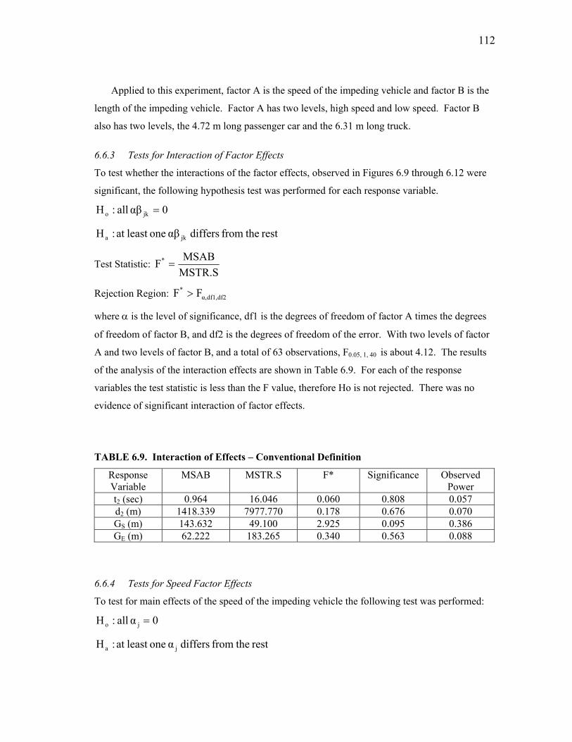
112
Applied to this experiment, factor A is the speed of the impeding vehicle and factor B is the
length of the impeding vehicle. Factor A has two levels, high speed and low speed. Factor B
also has two levels, the 4.72 m long passenger car and the 6.31 m long truck.
6.6.3 Tests for Interaction of Factor Effects
To test whether the interactions of the factor effects, observed in Figures 6.9 through 6.12 were
significant, the following hypothesis test was performed for each response variable.
0αβ all:H jko =
rest thefrom differs αβ oneleast at :H jka
Test Statistic: MSTR.SMSABF* =
Rejection Region: df2df1,α,* FF >
where α is the level of significance, df1 is the degrees of freedom of factor A times the degrees
of freedom of factor B, and df2 is the degrees of freedom of the error. With two levels of factor
A and two levels of factor B, and a total of 63 observations, F0.05, 1, 40 is about 4.12. The results
of the analysis of the interaction effects are shown in Table 6.9. For each of the response
variables the test statistic is less than the F value, therefore Ho is not rejected. There was no
evidence of significant interaction of factor effects.
TABLE 6.9. Interaction of Effects – Conventional Definition
Response Variable
MSAB MSTR.S F* Significance Observed Power
t2 (sec) 0.964 16.046 0.060 0.808 0.057 d2 (m) 1418.339 7977.770 0.178 0.676 0.070 GS (m) 143.632 49.100 2.925 0.095 0.386 GE (m) 62.222 183.265 0.340 0.563 0.088
6.6.4 Tests for Speed Factor Effects
To test for main effects of the speed of the impeding vehicle the following test was performed:
0α all:H jo =
rest thefrom differs α oneleast at :H ja

113
Test Statistic: MSTR.S
MSAF* =
Rejection Region: df2df1,α,* FF >
where df1 is the degrees of freedom of factor A and df2 is the degrees of freedom of the error.
F0.05, 1, 40 is about 4.12. The results of the test for main effects of the speed of the impeding
vehicle are shown in table 6.10. There was evidence to support a difference in the response
variables, distance in the left lane and end gap, based on the effect of the levels of the speed of
the impeding vehicle.
TABLE 6.10. Effect of the Impeding Vehicle Speed – Conventional Definition
Response Variable
MSA MSTR.S F* Significance Observed Power
t2 (sec) 62.011 16.046 3.865 0.056 0.484 d2 (m) 71847.809 7977.770 9.006 0.005 0.834 GS (m) 86.659 49.100 1.765 0.192 0.254 GE (m) 987.280 183.265 5.387 0.025 0.620
6.6.5 Tests for Length Factor Effects
To test for main effects of the length of the impeding vehicle the following test was performed:
0β all:H ko =
rest thefrom differs β oneleast at :H ka
Test Statistic: MSTR.S
MSBF* =
Rejection Region: df2df1,α,* FF >
where df1 is the degrees of freedom of factor B and df2 is the degrees of freedom of the error.
F0.05, 1, 40 is about 4.12. The results of the test for main effect are shown in Table 6.11. There
was evidence to support a difference in the response variables, time and distance in the left lane
and start gap, based on the effect of the levels of the length of the impeding vehicle.

114
TABLE 6.11. Effect of the Impeding Vehicle Length – Conventional Definition
Response Variable
MSB MSTR.S F* Significance Observed Power
t2 (sec) 408.191 16.046 25.439 <0.001 0.998 d2 (m) 172025.608 7977.770 21.563 <0.001 0.995 GS (m) 537.868 49.100 10.955 0.002 0.898 GE (m) 605.864 183.265 3.306 0.077 0.427
6.7 Analysis Results – Conventional Definition
The results from the data analysis were grouped by the response variables to describe the impact
of the speed and length of the impeding vehicle of passing behavior. These results are discussed
in terms of what was expected and what might have caused the observed behavior to differ from
those expectations.
6.7.1 Time in the Left Lane
As expected, the mean time in the left lane increased with increases in the speed and length of
the impeding vehicle. These relationships were illustrated on the factor effects plot in Figure
6.8. It appeared that there was an interaction between the factors but the interaction was found
not significant (F= 0.060, P=0.808).
The increase in the speed of the impeding vehicle was shown to increase the time traveled in
the left lane. From the factor effects plot in Figure 6.8, it appeared that this relationship was far
more pronounced when the impeding vehicle was a truck. There appeared to be very little
difference in the time in the left lane when the impeding vehicle was a car. The effect of the
speed was found not significant (F=3.865, P=0.056). The observed power of this test was 0.484.
A larger sample size could increase the power of the test and perhaps produce a significant effect
of the speed factor.
The lack of significance in the effect of the speed could be attributable to the small
difference between the fast and slow impeding vehicle speeds. One of the limitations of the
prototype was the presence of speed limit signs in the rural simulation environment. The
impeding vehicle needed to be traveling slower than the speed limit so that the test driver would
pass the vehicle but the difference could not be unrealistically large. Therefore, the fast and slow
vehicles were programmed to travel within 8 km/h (5 mph) and 16 km/h (10 mph) under the
speed limit respectively. Removing or changing the speed limit signs would provide the

115
opportunity to use a wider range of impeding vehicle speeds. A wider range of speeds could
result in larger and perhaps significant effects for the time in the left lane.
The effect of the length was significant (F=25.439, P<0.001). The time traveled in the left
lane was observed to be sensitive to the small difference in length between the 4.72 m long
passenger car and the 6.31 m truck.
6.7.2 Distance in the Left Lane
It was also expected that an increase in the speed or length if the impeding vehicle would
increase the distance traveled in the left lane. This relationship was illustrated in the factor
effects plot in Figure 6.9 and there appeared to be an interaction in the effects of the speed and
length of the impeding vehicle. This interaction was not significant (F=0.178, P=0.676).
The speed (F=9.006, P=0.005) and length (F=21.563, P<0.001) of the impeding vehicle
significantly increased the distance traveled in the left lane. The powers of these tests were
0.834 and 0.995 respectively for the effects of the speed and length of the impeding vehicle.
6.7.3 Start Gap Distance
It was expected that the test driver would leave a greater start gap distance when the impeding
vehicle traveled at the faster of the two speeds or when the impeding vehicle was a truck as
opposed to a car. These relationships were observed in the factor effects plot in Figure 6.10 and
there appeared to have been an interaction between the factor effects. However, this interaction
was not significant (F=2.925, P=0.095).
The effect of the speed of the impeding vehicle (F=1.765, P=0.192) was not significant. It
was surprising to see that when the impeding vehicle was a car, subjects left greater start gaps at
the faster speed than at the slower speeds. The opposite behavior was expected. The observed
power for the test of the effect of the speed of the impeding vehicles was 0.254. A larger sample
size could increase the power of the test and perhaps produce a significant effect of the speed
factor. The small differences in the speeds of the impeding vehicle may have also played a role.
Larger increases in the speed may also significantly affect the start gap distance.
The effect of the length of the impeding vehicle (F=10.955, P=0.002) was significant with an
observed power of 0.898. Whether the impeding vehicle was traveling at the slower or faster
speeds, the start gap was larger for the longer impeding vehicles. The distance in the left lane
was sensitive to the small difference in the lengths of the impeding vehicles.

116
6.7.4 End Gap Distance
It was also expected that the test driver would leave greater end gap distance when the impeding
vehicle traveled at the faster of the two speeds or when the impeding vehicle was a truck as
opposed to a car. The factor effects plot in Figure 6.11 illustrated the opposite relationships.
The observed end gap decreased with increases in the speed and length of the impeding vehicle
and there appeared to be an interaction between these effects. The interaction was not significant
(F=0.340, P=0.563).
The effect of the speed of the impeding vehicle (F=5.387, P=0.025) was significant, however
the observed end gap distances were smaller at the faster speeds, which is contrary to
expectation. The effect was more pronounced when the impeding vehicle was a truck as
opposed to a car, however the effect of the length of the impeding vehicle (F=3.306, P=0.077)
was not significant.
These unexpected relationships may be explained by the design of the experimental scenario.
The impeding vehicles were the leading car and following truck in each of the fast and slow
traveling platoons. When a truck was passed, the test driver needed to return to the right lane in
between the truck and the lead vehicle in the platoon. When the lead vehicle was passed, the test
driver returned to the right lane in front of the lead vehicle and there was no other vehicle ahead
to restrict the end gap distance the test driver allowed. Therefore, the smaller end gap distances
observed for the faster and longer vehicles might be the consequence of whether or not a vehicle
was present ahead of the impeding vehicle.
6.8 Data Reduction – Alternate Definition
To avoid including overly large start gap and end gap distances, the passing data was reduced
using an alternate definition of the time and distance in the left lane. The time ( ) and distance
( ) that the passing vehicle occupies the left lane was defined as:
2t&
2d&
beginning when the center of the vehicle crossed over the centerline as the passing vehicle
moved into the left lane; and
•
• ending when the center of the vehicle crossed over the centerline as the passing vehicle
moved back into the right lane.

117
The start gap ( ) was the distance from the front of the passing vehicle to the rear of the
impeding vehicle when the center of the passing vehicle crossed the centerline to move into the
left lane. The end gap ( ) was the distance from the rear of the passing vehicle to the front of
the impeding vehicle when the center of the passing vehicle crossed the centerline to move back
into the right lane.
SG&
EG&
The data from the experimental scenario under each of the four passing conditions for all of
the 24 test drivers was examined. The time and distance in the left lane, start gap distance, and
end gap distance for each of the 96 passing maneuvers is shown in Appendix K along with a
description of the impeding vehicle.
6.8.1 Data Exploration
The Kolmogorov-Smirnov (K-S) test for normality was applied to the data in Appendix K and
the results are shown in Table 6.12. At a 0.05 level of significance, the normal distribution was
not a good fit for the start gap or end gap distances for this sample of passing maneuvers.
TABLE 6.12. Normality Test Results for Time, Distance, and Gap Distances, N=96
Response Variable
n Mean σ Absolute Extreme Difference
K-S test statistic
Significance
2t& (sec) 64 20.05 10.76 0.202 1.617 0.011
2d& (m) 64 490.30 237.64 0.202 1.613 0.011
SG& (m) 64 23.49 12.19 0.155 1.242 0.092
EG& (m) 64 47.37 19.25 0.137 1.099 0.178
Note: n is the sample size and σ is the standard deviation.
To further explore these distributions, box plots of the start gap and end gap distances were
plotted. The plots are shown in Figure 6.12 and 6.13. From the box plots, there appears to be 2
extreme outliers; one in the start gap distance interval labeled by 65 meters and one in the end
gap distance interval labeled by 80 meters. These come from passing maneuvers 24F3 and
23F2, respectively. These maneuvers were excluded from further analysis.

118
Length, m
6.314.72
Star
t Gap
, m
70
60
50
40
30
20
10
0
-10
1
1122
FIGURE 6.12. Box plots of start gap distances.
Length, m
6.314.72
End
Gap
, m
100
80
60
40
20
0
2
2
FIGURE 6.13. Box plots of end gap distances.

119
To ensure that the response variables were normally distributed, passing maneuvers 29F4
and 23F3 were removed. The results of the Kolmogorov-Smirnov (K-S) test for normality for
the remaining 92 passing maneuvers are shown in Table 6.13. At the 0.05 level of significance,
the results of the K-S tests support that the normal distribution was a good fit for each of the
response variables for this sample of 92 passing maneuvers.
TABLE 6.13. Normality Test Results for Time, Distance, and Gap Distances, N=92
Response Variable
n Mean σ Absolute Extreme Difference
K-S test statistic
Significance
2t& (sec) 92 10.21 2.45 0.063 0.601 0.862
2d& (m) 92 263.49 61.54 0.067 0.646 0.798
SG& (m) 92 14.54 8.91 0.141 1.357 0.050
EG& (m) 92 27.42 8.73 0.080 0.772 0.591
Note: n is the sample size and σ is the standard deviation.
TABLE 6.14. Time, Distance, and Gap Distances – Alternate Definition
Slow Speed Fast Speed All Speeds Response Variable
Impeding Vehicle n Mean σ n Mean σ n Mean σ car 22 8.59 1.38 24 9.60 2.21 46 9.12 1.91 truck 23 10.89 1.75 23 11.73 2.99 46 11.31 2.46 2t& (sec) all 45 9.76 1.95 47 10.64 2.81 92 10.21 2.45 car 22 219.2 32.2 24 256.8 57.3 46 238.8 50.2 truck 23 268.9 39.4 23 307.3 75.0 46 288.1 62.3 2d& (m) all 45 244.6 43.6 47 281.5 70.6 92 263.4 61.5 car 22 11.12 7.87 24 12.47 8.46 46 11.82 8.12 truck 23 15.46 8.52 23 19.04 9.13 46 17.25 8.92 SG& (m) all 45 13.33 8.40 47 15.69 9.31 92 14.54 8.91 car 22 30.64 9.36 24 27.68 9.06 46 29.10 9.27 truck 23 27.78 7.48 23 23.70 7.96 46 25.74 7.91 EG& (m) All 45 29.18 8.47 47 25.73 8.74 92 27.42 8.73
Note: n is the sample size and σ is the standard deviation.

120
6.8.2 Data Summary
The averages and standard deviations of the times and distances in the left lane, start gap and end
gap distances are presented in Table 6.14. As expected, it appears that the time and distance in
the left lane were greater when the impeding vehicle was a truck as opposed to a car or when the
impeding vehicle was traveling at the faster of the two speeds. The start gap distance was also
greater when the impeding was a truck or traveling at the faster speed. Contrary to expectation
was the decrease in the end gap distances when the impeding vehicle was a truck as opposed to a
car or when the impeding vehicle was traveling at the faster of the two speeds.
6.9 Data Analysis – Alternate Definition
The effects of the speed and length of the impeding vehicle on each of the response variables
was examined using factor effects plots and then tested using F-tests for the ANOVA model
presented in section 6.6.2.
6.9.1 Factor Effect Plots
The factor effect plots for the time and distance in the left lane, start gap and end gap distances
are shown in Figures 6.14 through 6.17.
Length, m
6.314.72
Mea
n Ti
me,
s
12.0
11.5
11.0
10.5
10.0
9.5
9.0
8.5
8.0
Speed
fast
slow
FIGURE 6.14. Alternate factor effects plot for time in the left lane.

121
Length, m
6.314.72
Mea
n D
ista
nce,
m
320
300
280
260
240
220
200
Speed
fast
slow
FIGURE 6.15. Alternate factor effects plot for distance in the left lane.
Length, m
6.314.72
Mea
n St
art G
ap, m
20
18
16
14
12
10
Speed
fast
slow
FIGURE 6.16. Alternate factor effects plot for start gap distances.

122
Length, m
6.314.72
Mea
n En
d G
ap, m
32
30
28
26
24
22
Speed
fast
slow
FIGURE 6.17. Alternate factor effects plot for end gap distances.
From the factor effects plots, there appears to have been little if any interaction between the
effects of the speed of the impeding vehicles and the effects of the length of the impeding
vehicle. These relationships were further explored by conducting F-tests for the strengths of
interaction between the factor effects as well as the main factor effects.
6.9.2 Tests for Interaction of Factor Effects
The same procedures for testing the interaction of factor effects that was used in section 6.6.3
were applied. The results of the ANOVA are shown in Tables 6.15. The interaction of the
factor effects were not significant given that F0.05, 1, 65 is slightly less than 4.
TABLE 6.15. Interaction of Effects – Alternate Definition
Response Variable MSAB MSTR.S F* Significance Observed Power 2t& (sec) 0.039 2.907 0.013 0.908 0.052
2d& (m) 71.663 1624.004 0.044 0.834 0.055
SG& (m) 69.995 24.458 2.862 0.095 0.385
EG& (m) 11.962 38.600 0.310 0.580 0.085

123
6.9.3 Tests for Speed Factor Effects
The main effects of the impeding vehicle speed were tested using the procedures outlined in
Section 6.6.4 and the results are shown in Table 6.16. The effect of the impeding vehicle speed
was significant for the distance in the left lane and the end gap distance.
TABLE 6.16. Effects of the Impeding Vehicle Speed – Alternate Definition
Response Variable MSA MSTR.S F* Significance Observed Power 2t& (sec) 10.920 2.907 3.757 0.057 0.480
2d& (m) 23017.263 1624.004 14.173 <0.001 0.960
SG& (m) 63.742 24.458 2.606 0.111 0.356
EG& (m) 322.094 38.600 8.344 0.005 0.812
6.9.4 Tests for Length Factor Effects
The main effects of the impeding vehicle length were tested using the procedures outlined in
Section 6.6.5 and the results are shown in Table 6.17. The effect of the impeding vehicle speed
was significant for each of the response variables.
TABLE 6.17. Effects of the Impeding Vehicle Length – Alternate Definition
Response Variable MSB MSTR.S F* Significance Observed Power 2t& (sec) 106.393 2.907 36.602 <0.001 1.000
2d& (m) 54454.633 1624.004 33.531 <0.001 1.000
SG& (m) 671.732 24.458 27.465 <0.001 0.999
EG& (m) 300.498 38.600 7.785 0.007 0.785
6.10 Results of the Data Analysis – Alternate Definition
The results of the alternate data analysis are presented in the following sections grouped by the
various response variables.

124
6.10.1 Time in the Left Lane
It was expected that an increase in the speed or length of the impeding vehicle would increase
the time traveled in the left lane. In the factor effect plot in Figure 6.14, the time in the left lane
was shown to increase for greater speeds and vehicle lengths. There was no significant
interaction of these effects (F=0.013, P=0.908).
As the speed increases, the time in the left lane increases. This relationship was not
significant (F=3.757, P=0.057) but the observed power of the test was 0.480. Increasing the
sample size would increase the observed power of the test and might produce a significant effect
of the speed factor. The lack of significance in the effect of the speed could also be attributable
to the small difference between the fast and slow impeding vehicle speeds as discussed in section
6.7.1.
The effect of the length was significant (F=36.602, P<0.001). The time traveled in the left
lane was observed to be sensitive to the small difference between the 4.72 m long passenger car
and the 6.31 m truck.
6.10.2 Distance in the Left Lane
It was also expected that an increase in the speed or length of the impeding vehicle would
increase the distance traveled in the left lane. In the factor effects plot in Figure 6.15, the
distance in the left lane was shown to increase with increases in the speed and length of the
impeding vehicle. There was no significant interaction of these effects (F=0.044, P=0.834),
however increasing the speed (F=14.173, P<0.001) and the length (F=33.531, P<0.001) of the
impeding vehicle significantly increased the distance traveled in the left lane.
6.10.3 Start Gap Distance
It was expected that the test driver would leave a greater start gap distance when the impeding
vehicle traveled at the faster of the two speeds or when the impeding vehicle was a truck as
opposed to a car. In the effects plot in Figure 6.16, there appeared to be some interaction
between the effects of the speed and the length of the impeding vehicle. The interaction was not
significant (F=2.862, P=0.095).
The test drivers left a greater start gap distance for the faster impeding vehicles but the effect
was not significant (F=2.606, P=0.111). The test drivers also left a greater start gap distance for
the longer vehicles. The effect of the impeding vehicle length was significant (F=27.465,
P<0.001).

125
6.10.4 End Gap Distance
It was also expected that the test driver would leave greater end gap distance when the impeding
vehicle traveled at the faster of the two speeds or when the impeding vehicle was a truck as
opposed to a car. In the factor effects plot in Figure 6.17 it is seen that the reverse relationship
occurred. The test drivers left significantly larger end gap distances when the impeding vehicle
was traveling at the slower speed (F=8.344, P=0.005) or when the impeding vehicle was a car
(F=7.785, P=0.007). This is likely explained by the design of the experimental scenario and the
presence or absence of a vehicle in front of the impeding vehicle, as discussed in section 6.7.4.
There was no significant interaction of these effects (F0.310, P=0.580).
6.11 Comparison of Data Analyses (Conventional and Alternate Definitions)
Two definitions were used to define the time and distance in the left lane and the start and end
gap distances. This was possible because the comprehensive data that was captured during the
passing study, and estimated from the VISSIM data, detailed the movements of all the vehicles
for every tenth of a second. In both approaches, the position of the passing vehicle was
referenced to the centerline of the roadway. Using the conventional definition, the front left and
the rear left wheels of the passing vehicle were referenced, while using the alternate definition,
the center of the vehicle was referenced.
In both analyses, the interaction between the speed effects and the length effects was not
significant. For the main effects, the p-values for each of the response variables are included in
Table 6.18. There were no differences in the significance of the main effects however there were
changes in the p-values.
TABLE 6.18. Comparison of Results – Conventional and Alternate Definitions
Conventional Definition Alternate Definition
Response Variable
Speed Effect
Length Effect
Response Variable
Speed Effect
Length Effect
t2 (sec) 0.056 <0.001* 2t& (sec) 0.057 <0.001*
d2 (m) 0.005* <0.001* 2d& (m) <0.001* <0.001*
GS (m) 0.192 0.002* SG& (m) 0.111 <0.001*
GE (m) 0.025* 0.007* EG& (m) 0.005* 0.007*
Significant effects are indicated with an asterisk.

126
6.12 Nonparametric Analysis
In sections 6.5.1 and 6.8.1, outliers in the passing data were removed from the data sets to obtain
distributions of the response variables that resembled a normal distribution. This was necessary
because when applying of the ANOVA procedures, it was assumed that each group of data was
an independent random sample from a normal population. A preferred alternative to excluding
the outliers and using ANOVA procedures was to analyze the data using nonparametric
techniques.
The Friedman test is the nonparametric equivalent of a one-sample repeated measures
design, which was used to test that
Ho: all experimental conditions had identical effects
Ha: at least on experimental condition tended to yield larger effects than another experimental
condition.
The k variables were ranked from 1 to k and the ranks were used to calculate the test statistic T,
which was then compared to the Chi-squared distribution, with (k-1) degrees of freedom. If
there was evidence that the experimental conditions were not identical, then differences were
tested using the Wilcoxon signed rank test. The differences were considered significant when
the p-value was less than or equal to 0.05. These tests were applied to the passing data
summarized using both the conventional and alternate definitions.
6.12.1 Conventional Definition
The time and distance in the left lane, start gap distance, and end gap distance for each of the 64
passing maneuvers shown in Appendix J were analyzed using the Friedman and Wilcoxon
nonparametric tests. The resulting p-values are shown in Table 6.19. Although the p-values
varied from those found using the ANOVA procedures, the significance of the effects was
comparable.
TABLE 6.19. Nonparametric Results Using the Conventional Definition
Response Variable Group Differences Speed Effect Length Effect t2 (sec) 0.001* 0.085 0.001* d2 (m) <0.001* 0.012* 0.001* GS (m) 0.003* 0.866 0.001* GE (m) 0.013* 0.050* 0.010*
Significant effects are indicated with an asterisk.

127
6.12.2 Alternate Definition
The time and distance in the left lane, start gap distance, and end gap distance for each of the 96
passing maneuvers shown in Appendix K were analyzed using the Friedman and Wilcoxon
nonparametric tests. The resulting p-values are shown in Table 6.20. Although the p-values
varied from those found using the ANOVA procedures, the significance of the effects was
comparable.
TABLE 6.20. Nonparametric Results Using the Alternate Definition
Response Variable Group Differences Speed Effect Length Effect 2t& (sec) <0.001* 0.208 <0.001*
2d& (m) <0.001* 0.003* <0.001*
SG& (m) <0.001* 0.103 <0.001*
EG& (m) 0.025* 0.002* 0.002*
Significant effects are indicated with an asterisk.
6.12.3 Results of the Nonparametric Analyses
Using the Friedman and Wilcoxon nonparametric tests, the impact of the speed of the impeding
vehicle on the distance in the left lane and the end gap distance, and the impact of the length of
the impeding vehicle on the distance and time in the left lane, as well as both the start gap and
end gap distances was found to be significant. The significance of the effects was comparable
using the conventional and alternate definitions, although the p-values varied. The significance
of the effects was also comparable to those found using the ANOVA procedures.
6.13 Transferability of Results
There are concerns about the transferability of simulator study results to the real world. Drivers
in a simulated environment may behave differently than in the real world, may be affected by the
symptoms of simulator sickness, and may have difficulties controlling the simulated vehicles or
maneuvering in the simulated environment. To determine whether this prototype was suitable
for studying passing behavior, the results using both the conventional and the alternate
definitions were compared to the field observations reported by Polus et al. (22).

128
6.13.1 Results Using the Conventional Definition
In this section, the passing data summarized using the conventional definition was compared to
the previously reported field data. The means, standard deviations, and sample sizes for the time
and distance in the left lane and the start and end gap distances are shown in Table 6.21.
The average time in the left lane and the average distance traveled in the left lane were
approximately double that of the field observations. Similarly, the average start gap distance
was approximately triple that of the field observations and the average end gap distance was
approximately double that of the field observations.
TABLE 6.21. Comparing the Conventional Definition Results with Field Observations
Results Field Observations Response Variable Mean σ n Mean σ n
Time in left lane (s) 19.23 8.63 63 10.9 3.4 527 Distance in left lane (m) 472.28 190.43 63 253.7 80.9 507 Start gap distance (m) 23.45 12.29 63 7.4 6.1 462 End gap distance (m) 47.31 19.40 63 21.3 9.7 451
Note: n is the sample size and σ is the standard deviation.
To test whether the underlying populations of these samples are the same, tests for the
difference of means were performed.
0µµ:H yxo =−
Test Statistic:
ms
ns
0yxzy
2x
2
+
−−=
where the population variances were estimated by the sample variances (s2) with sample sizes n
and m. The observed test statistics were:
|z| = 7.59 for the time in the left lane;
|z| = 9.01 for the distance in the left lane;
|z| = 10.20 for the start gap distance; and
|z| = 10.46 for the end gap distance.

129
In each case, the null hypothesis was rejected at an approximate significance level of 0.05 (z0.025
= 1.96), and the conclusion was that the simulation data and the field data were from different
populations.
6.13.2 Results Using the Alternate Definition
In this section, the passing data summarized using the alternate definition was compared to the
previously reported field results. The means, standard deviations, and sample sizes for the time
and distance in the left lane and the start gap and end gap distances are shown in Table 6.22.
The analysis results, based on the alternate definition, compare better to the field
observations reported by Polus et al. (22) than do the results based on the conventional
definition. The average time in the left lane and the average distance traveled in the left lane
appear to be comparable to the field observations. The average start gap distance is
approximately double that of the field observations and the average end gap distance is slightly
greater than the field observations.
TABLE 6.22. Comparing the Alternate Definition Results with Field Observations
Alternate Results Field Observations Response Variable Mean σ n Mean σ n
Time in left lane (s) 10.21 2.45 92 10.9 3.4 527 Distance in left lane (m) 263.49 61.54 92 253.7 80.9 507 Start gap distance (m) 14.54 8.91 92 7.4 6.1 462 End gap distance (m) 27.42 8.73 92 21.3 9.7 451
Note: n is the sample size and σ is the standard deviation.
To test whether the underlying populations of these samples are the same, the same test used
in the previous section were applied to test for the difference of means. The observed test
statistics were:
|z| = 2.34 for the time in the left lane
|z| = 1.33 for the distance in the left lane
|z| = 7.35 for the start gap distance
|z| = 6.01 for the end gap distance
130
At an approximate level of significance of 0.05 (z0.025 = 1.96), there was evidence that the mean
distance in the left lane was the same therefore the null hypothesis was not rejected. However,
the null hypothesis was rejected for the time in the left lane, and the start gap and end gap
distances. The simulation data and field data were from different populations.
From the results of the passing study, using both definitions, and comparisons with previous
field observations, it appears that the drivers left more space between vehicles when in the
simulated environment. Three possible reasons for these differences between the simulation data
and the field data are discussed in the following sections.
6.13.3 Distance Judgments in Real and Simulated Environments
The first reason for the differences is the difficulties drivers have judging the perceived distance
in real and simulated environments. In a fixed-based driving simulator, such as the one used in
this research, a test driver views the two-dimensional image from a fixed point. There are no
vestibular cues and the perception of depth, or stereopsis resulting from binocular disparity is not
possible. The test driver must rely on monocular cues for depth perception. These cues include
atmospheric perspective, relative height, relative size, shadows, texture gradient, occlusion, and
motion parallax (59) and are provided by how the images are drawn.
Pertinent to this experiment, is a comparative study, which investigated the judgment of the
safe distance to a lead vehicle. The distance judgments made in the simulated environment were
underestimated compared to those made while driving in the real world (171). In several other
comparative studies, the tendency to underestimate distances has been shown to be more severe
in virtual environments as compared to the real world (172, 173, 174). If the test drivers in this
passing study underestimated the distance to the impeding vehicle, that would account for the
large start gap and end gap distances, and consequently the large distances and times in the left
lane.
6.13.4 Lateral Position
The second reason for the differences could stem from the lateral position of the test vehicle. In
the passing study, five test drivers performed at least one pass, where the test vehicle was
partially in the left lane while the test driver waited for an opportunity to pass. Six test drivers
performed at least one pass where the test vehicle remained in the left lane at the end of the pass
until after the opposing vehicle passed. Although the data for these test drivers was removed
from the analysis, they may be indicative of a more generalized problem.

131
The images in the simulated environment were two-dimensional. To better see around the
impeding vehicle required driving the vehicle further to the left and perhaps crossing the
centerline. In a real environment, this is a risky behavior but in the simulated environment there
is no imminent threat from the opposing vehicles. Because of the lack of consequences, drivers
may have been encouraged to accept what would normally be considered risky or inappropriate
situations.
6.13.5 Bias in Field Data
The third reason for the differences could be from how the data was collected in the field.
Considering the difficulties accurately pinpointing when and where the vehicle first begins to
cross the centerline as it moves into the left lane or returns to the right lane, it is possible that the
field data reflects a passing maneuver that falls somewhere between the conventional and
alternate definitions. This reason is supported by the fact that the mean distance in the left lane
for the alternate definition and the field data were the same.

132
7 PASSING BEHAVIOR
The data collected during the passing study was further examined to illustrate the variability in
how the passing maneuver is performed and the variability in the types of passing maneuvers.
7.1 Driver Variability
During the passing study, the sex of the test driver was collected. It was recorded on the
simulator sickness questionnaire and used in the naming convention adopted for the data files, as
described in Section 6.5. The effect of the sex of the test drivers was examined using the data in
Appendix J. The data was grouped by the sex of the test drivers and the differences in the time
and distance in the left lane, and the start and end gap distances were evaluated using the
Friedman test and the Wilcoxon nonparametric, signed ranks test. Compared to the male test
drivers, the time in the left lane (P=0.067), distance in the left lane (P=0.067), start gap distance
(P=0.909), and end gap distance (P=0.006) were greater for the female test drivers. The
difference in the end gap distance was significant, at a 0.05 level of significance.
7.2 Position of the Passing Vehicle Relative to the Impeding Vehicle
To avoid a collision, the driver maintained some minimum or safe distance away from the
impeding vehicle. The variability in the start gap and end gap distances was examined.
7.2.1 Start Gap
The start gap (GS) was the distance from the front bumper of the passing vehicle to the rear
bumper of the impeding vehicle at the moment the passing vehicle began to enter the left lane. It
was calculated from the positions of the impeding (xi) and passing (xp) vehicles, taking account
of the vehicle lengths (Li and Lp) such that:
+−
−=
2L
x2L
xG pp
iiS (7.1)
The frequency distribution of the start gap distance is shown in Figure 7.1. Using the
Kolmogorov-Smirnov test (Z=1.242), the start gap distance was shown to resemble a normal
distribution with a mean of 23.5 m and a standard deviation of 12.19 m.

133
Start Gap, m
75.0
65.0
55.0
45.0
35.0
25.0
15.05.0
Freq
uenc
y
16
14
12
10
8
6
4
2
0
Std. Dev = 12.19 Mean = 23.5N = 64.00
FIGURE 7.1. Frequency distribution of the start gap distances.
7.2.2 End Gap
The end gap (GE) was the distance from the rear bumper of the passing vehicle to the front
bumper of the impeding vehicle at the moment the passing vehicle completely returned to the
right lane. It was also calculated from the positions of the impeding (xi) and passing (xp)
vehicles, taking account of the vehicle lengths (Li and Lp) such that:
+−
−=
2L
x2
LxG i
ip
pE (7.2)
The frequency distribution of the end gap is shown in Figure 7.2. Using the Kolmogorov-
Smirnov test (Z=1.099), the end gap distance was shown to resemble a normal distribution with
a mean of 47.4 m and a standard deviation of 19.25 m.

134
End Gap, m
100.
0
90.0
80.0
70.0
60.0
50.0
40.0
30.0
20.0
Freq
uenc
y
12
10
8
6
4
2
0
Std. Dev = 19.25 Mean = 47.4N = 64.00
FIGURE 7.2. Frequency distribution of the end gap distances.
7.3 Speed of the Passing Vehicle
The driver controlled the longitudinal position of the vehicle through speed inputs. The speed of
the passing vehicle can be described in terms of the absolute speed gain that was attained during
the passing maneuver. It can also be described as the maximum speed difference with respect to
the impeding vehicle or relative to the speed limit. The variability of the speed of the passing
vehicle was examined using each of these descriptions.
7.3.1 Speed Gain
The speed gain of the passing vehicle was calculated by a comparison of its maximum and
minimum speeds. The minimum speed occurred when acceleration began (sp(accel)), and the
maximum speed occurred when deceleration began (sp(decel)). The speed gain (∆sp) was
calculated as:
(accel)s(decel)s∆s ppp −= (7.3)

135
The distribution of the speed gain of the passing vehicle for the 96 passing maneuvers is shown
in Figure 7.3. Using the Kolmogorov-Smirnov test (Z=0.853), the speed gain was shown to
resemble a normal distribution with a mean of 7.7 m/s and a standard deviation of 2.29 m/s.
Speed Gain, m/s
15.0
13.0
11.09.0
7.0
5.0
3.0
1.0
Freq
uenc
y
30
20
10
0
Std. Dev = 2.29 Mean = 7.7N = 96.00
FIGURE 7.3. The frequency distribution of the speed gain of the passing vehicle.
The range in speed gain was quite large, with the speed of the passing vehicle increased as
much as 16 m/s (57.6 km/h or 36 mph). The speed of the passing vehicle needed to be compared
to the speed of the impeding vehicle to get a better feel for how the passing maneuver was
performed.
7.3.2 Maximum Speed Difference
The maximum speed difference was the maximum speed of the passing vehicle relative to the
speed of the impeding vehicle. The passing vehicle reached its maximum speed at the moment it
began to decelerate. The speed of the passing vehicle (sp(decel)) and the impeding vehicle
(si(decel)) at that moment were compared to determine the speed of the passing vehicle relative
to the impeding vehicle (Spi(decel)), such that

136
(decel)s(decel)s(decel)S ippi −= (7.4)
The distribution of the maximum speed difference is shown in Figure 7.4. Using the
Kolmogorov-Smirnov test (Z=0.851), the maximum speed difference was shown to resemble a
normal distribution with a mean of 7.8 m/s and a standard deviation of 1.90 m/s.
Maximum Speed Difference, m/s
12.0
11.0
10.09.0
8.0
7.0
6.0
5.0
4.0
Freq
uenc
y
14
12
10
8
6
4
2
0
Std. Dev = 1.90 Mean = 7.8N = 96.00
FIGURE 7.4. The frequency distribution of the maximum speed differences.
Considering that the impeding vehicles were traveling between 19 m/s (43 mph) and 22.2
m/s (50 mph), and the speed limit was 24.4 m/s (55 mph), the range in the maximum speed
difference was quite large. During some passes, the passing vehicle reached a speed as much as
50% faster than the impeding vehicle. These speed differences suggest that the speed limit was
exceeded during many of the passing maneuvers.
7.3.3 Exceeding the Speed Limit
The frequency of the maximum speed (sp(decel))of the passing vehicle was plotted and is shown
in Figure 7.5. In each of the 96 passing maneuvers, the passing vehicle exceeded the 24.4 m/s

137
(55 mph) speed limit. In 29 passing maneuvers, the speed limit was exceeded by at least 4.4 m/s
(10 mph) and in one passing maneuver the speed limit was exceeded by 9.4 m/s (21 mph).
Speed of Passing Vehicle, m/s
33.0
32.0
31.0
30.0
29.0
28.0
27.0
26.0
25.0
Freq
uenc
y
14
12
10
8
6
4
2
0
Std. Dev = 1.85 Mean = 28.1N = 96.00
FIGURE 7.5. The frequency distribution of passing vehicle maximum speeds.
The speed of the passing vehicle has been described as the absolute speed gain, the
maximum speed difference with respect to the impeding vehicle, and the maximum speed in
excess of the speed limit. The speed of the passing vehicle was directly related to the
acceleration and deceleration behavior of the driver. As the magnitude and duration of the
acceleration increased, the speed increased. To further explore the variation in how the passing
maneuver was performed, the acceleration and deceleration behavior was examined.
7.4 Acceleration and Deceleration Behavior.
For each of the 96 passing maneuvers, the data was examined to identify when the passing driver
began to accelerate and began to decelerate. Each was identified in relation to the following
instances.
1. The passing vehicle began to enter the left lane;
2. The passing vehicle was completely in the left lane;

138
3. The passing vehicle was abreast of the impeding vehicle;
4. The passing vehicle began to enter the right lane; and
5. The passing vehicle was completely in the right lane.
These instances are illustrated and numbered accordingly in Figure 7.6. The beginning of the
acceleration is shown in green and beginning of the deceleration is shown in red.
FIGURE 7.6. The order tasks were performed during the passing maneuvers.
In 46 passes the acceleration began prior to the vehicle moving into the left lane (before
instance 1) and in 49 passes the acceleration began as the vehicle moved into the left lane
(between instances 1 and 2). For one pass, acceleration did not begin until the vehicle was
completely in the left lane (between instances 2 and 3).
In 13 passes, deceleration began prior to the vehicle coming abreast with the impeding
vehicle (between instances 2 and 3). In 43 passes, deceleration began prior to the vehicle
moving back into the right lane (between instances 3 and 4), followed by 29 passes where
deceleration began as the vehicle moved back into the right lane (between instances 4 and 5). In
12 passes the drivers began to decelerate only after completely returning to the right lane (after
instance 5). To further explore the acceleration behavior of the drivers, the duration and
magnitude of the acceleration was examined. The results are presented in the following two
sections.

139
7.4.1 Acceleration Duration
The acceleration duration was calculated as the time between the moment acceleration began
(tp(accel)) and the moment deceleration began (tp(decel)). The frequency distribution of the
acceleration duration is shown in Figure 7.7. Using the Kolmogorov-Smirnov test (Z=0.670),
the duration of acceleration was shown to resemble a normal distribution with a mean of 13.3 s
and a standard deviation of 4.04 s.
Duration of Acceleration, s
22.0
20.0
18.0
16.0
14.0
12.0
10.08.0
6.0
4.0
Freq
uenc
y
14
12
10
8
6
4
2
0
Std. Dev = 4.04 Mean = 13.3N = 96.00
FIGURE 7.7. Frequency distribution of the duration of acceleration.
7.4.2 Acceleration Magnitude
The acceleration magnitude was limited by the performance capabilities of the simulation
vehicle. The acceleration performance was shown in Figure 4.8. At the speed limit of 24.4 m/s
(55 mph or 88 km/h) the maximum acceleration was approximately 1.5 m/s2. The acceleration
magnitude was represented by the average acceleration of the passing vehicle (āp). It was
calculated using the speed gain (∆sp) of the passing vehicle and the acceleration duration such
that:

140
(accel)t(decel)t∆s
a pp −
= (7.5)
The distribution of average acceleration achieved over the duration of acceleration is shown in
Figure 7.8. Using the Kolmogorov-Smirnov test (Z=0.670), the average acceleration was shown
to resemble a normal distribution with a mean of 0.60 m/s2 and a standard deviation of 0.17 m/s2.
Average Acceleration, m/s/s
1.13
1.06
1.00.94
.88
.81
.75
.69
.63
.56
.50
.44
.38
.31
Freq
uenc
y
20
10
0
Std. Dev = .17 Mean = .60N = 96.00
FIGURE 7.8. Frequency distribution of the magnitude of acceleration.
7.4.3 Discussion
The data from 96 passing maneuvers collected during the passing study was explored. In each
pass, the driver moved from the right lane to the left lane, overtook the impeding vehicle by
traveling at a higher speed, and moved back into the right lane. However, the drivers’ control of
the vehicle varied, as described by the range in the end gap and start gap distances, speed gain,
maximum speed difference, and acceleration duration and magnitude.
A portion of the variation may have been attributable to differences in the passing
conditions. Even though each driver was given the same experiment where the vehicle,

141
roadway, traffic, and environment conditions were controlled, the passing conditions that were
experienced were the result of the driver’s own behavior. For instance, the driver chose what
distance to follow the impeding vehicle and what gap to accept in the opposing traffic. Two
drivers maintaining different car following distances and choosing different sized gaps would
experience different passing conditions. It is for that reason that the driver behavior data was
used to examine the variability in the type of passing maneuver.
7.5 Variability in the Types of Passing Maneuver
Historically, passing maneuvers have been classified by the beginning and end of the maneuver
whereby the beginning is described as a flying start (5) or accelerated start (5) and the end is
described as a voluntary return (5) or forced return (5). An accelerated start has also been
described as a delayed start (9), and a forced return has also referred to as a hurried return (5, 9).
Using this classification system, the observer judges which category each passing maneuver
belongs. Because the descriptions are, by necessity qualitative, their own passing behavior and
their interpretation of the individual passing situations when making these judgments would
likely bias their judgments.
By using two categories, for the description of the beginning and end of the maneuver, it is
assumed that these categories are distinctly different. In the following sections, the data for 96
passing maneuvers recorded during the passing experiment was explored. By examining the
driver behavior at the beginning and end of the maneuver, it was found that the categories are not
distinct or easily distinguishable.
7.5.1 Start of the Passing Maneuver
A flying start is when the passing vehicle does not significantly slow down as it approaches and
overtakes the impeding vehicle. An accelerated start is when the passing vehicle is traveling at
about the same speed as the impeding vehicle and accelerates to overtake the impeding vehicle.
The passing vehicle may have traveled behind the impeding vehicle for some time or may have
recently approached and slowed to await a passing opportunity.
The difficulty with this classification is determining which definition best describes the start
of each passing maneuver. A flying start would have a high relative speed between the passing
and impeding vehicles and the amount of speed gained during the pass would be low.
Conversely, an accelerated start would have a low relative speed and a high speed gain. To

142
examine the relationship between the relative speed and the speed gain, the data from the passing
study was explored.
For each passing maneuver, the moment the passing vehicle began to accelerate was found,
and the speeds of the passing (sp(accel)) and impeding (si(accel)) vehicles was used to calculate
the speed of the passing vehicle relative to the impeding vehicle (Spi(accel)) as follows:
(accel)s(accel)s(accel)S ippi −= (7.6)
The maximum speed of the passing vehicle during the pass, otherwise the speed at the moment
when the passing vehicle begins to decelerate (sp(decel)) after overtaking the impeding vehicle,
was found and the speed gain (∆sp) was calculated as:
(accel)s(decel)s∆s ppp −= (7.7)
A plot of the relative speed versus the speed gain is shown in Figure 7.9.
Relative Speed, m/s
181614121086420
Spee
d ga
in, m
/s
6
4
2
0
-2
-4
-6
FIGURE 7.9. Relative speed (Spi(accel)) versus speed gain (∆sp).

143
Because the passing study was designed to elicit accelerated starts, the majority of the data
passing maneuvers began with a low relative speed. However, there appears to have been a
relationship between the relative speed and the speed gain. To examine this relationship, a linear
regression analysis was performed. The regression line is described by the following equation:
(accel)S 1.0587.748∆s pip −= (7.8)
Using a regression ANOVA, it was found that at a 0.05 level of significance, the relative speed
explains a good amount of the variation in the speed gain (F1,94≈3.95). The results of the
regression ANOVA are shown in Table 7.1.
TABLE 7.1. Regression ANOVA Results
Model Sum of Squares df Mean Square F-statistic Regression 192.861 1 192.861 59.151 Residual 306.485 94 3.260 Total 499.347 95
This relationship does not support the idea that there are two distinctly different categories to
describe the beginning of the passing maneuver. Instead, this relationship is evidence that there
is a continuum between accelerated and flying starts. To further examine this continuum,
additional passing data is needed; including passes that start with large relative speeds. In
addition, it is also desirable to confirm these findings with field data. The simulated
environment may have influenced the passing behavior during the study and that may have had
an impact on the strength of the relationship between the relative speed and the speed gain.
7.5.2 End of the Passing Maneuver
Historically, the presence of an opposing vehicle has been used to determine whether the end of
the pass was voluntary or forced. It was assumed that with an opposing vehicle, the passing
vehicle was hurried or forced to return to the right lane and without an opposing vehicle, the
passing vehicle returned to the right lane voluntarily. A crude interpretation of these definitions,
could lead to a voluntary return pass being mistakenly classified as forced return pass when an
opposing vehicle is present but does not pose a threat.

144
To examine the perceived threat of an opposing vehicle on the completion of a passing
maneuver, the data from the passing study was explored. It was assumed that the passing vehicle
decelerated only when the driver was comfortable with the clearance to the opposing vehicle and
confident that the pass would be completed. Therefore, the correlation between the clearance
(C(decel)) with the opposing vehicle and the relative position Xpi(decel) with the impeding
vehicle at the moment of deceleration was investigated.
For each passing maneuver, the moment the passing vehicle began to decelerate after
overtaking the impeding vehicle was identified. The head-on clearance (C(decel)) was
calculated from the estimated position of the opposing vehicle ( (decel)) (refer to section
6.4.2) and the position of the passing vehicle (x
ox
p(decel)), as:
[ ]2L
pop(decel)x(decel)xC(decel) −−= (7.9)
The 2Lp term was the distance from the center to the front bumper of the passing vehicle, and
was needed because the position was recorded with reference to the center of the vehicle. The
relative position (Xpi(decel)) was calculated from the positions of the front bumpers of the
impeding (xi(decel)) and passing (xp(decel)) vehicles as follows:
( ) ( )[ ]2L
i2L
ppiip (decelx(decel)x(decel)X +−+= (7.10)
A plot of the clearance with the opposing vehicle versus the relative position with the
impeding is shown in Figure 7.10. The data points where the clearance was greater than 500 m,
the opposing vehicle was not visible to the test driver, as discussed in section 6.3.2. The passes
represented by these data points, were voluntary return passes because there was no threat of an
opposing vehicle when the driver began to decelerate. Some drivers began to decelerate before
attaining a positive relative position with the impeding vehicle, and completed the maneuver
given the available clearance to the opposing vehicle. In these cases, the threat of the opposing
vehicle was low and the return to the right lane was voluntary. The remaining passing
maneuvers were more difficult to categorize. The correlation between the clearance with the
opposing vehicle and the relative position with the impeding vehicle for passes where the
impeding vehicle posed some threat is shown in Figure 7.11. The lane that was occupied at the
time of deceleration is labeled.

145
Relative Position with Impeding Vehicle, m
140120100806040200-20-40
Cle
aran
ce w
ith O
ppos
ing
Veh
icle
, m
1200
1000
800
600
400
200
0
-200
-400-600
FIGURE 7.10. Clearance versus relative position at the moment of deceleration.
Relative Position with Impeding Vehicle, m
140120
10080
6040
200
-20
Cle
aran
ce w
ith O
ppos
ing
Veh
icle
, m
500
300
100
-100
-300
-500
Lane Occupied
Right
Left
Both
FIGURE 7.11. Lane occupied at the moment of deceleration.

146
With the assumption that the driver decelerated only when comfortable with the clearance to
the opposing vehicle and confident that the pass would be completed, it was expected that every
driver would decelerate prior to the opposing vehicle passing by and prior to returning to the
right lane. There were a couple unexpected behaviors that occurred that should be pointed out.
Some drivers did not decelerate until after the opposing vehicle had passed, as noted by those
data points where the clearance is negative. Even though the impeding vehicle had been
successfully overtaken and the threat of the opposing vehicle was gone, both of which should
have elicited the driver to decelerate, some drivers continued to travel at a high speed. In
addition, some drivers had not completely returned to the right lane by the time the opposing
vehicle passed by even though they were well ahead of the impeding vehicle. The reasons for
these behaviors were not clear. It could have been linked to the difficulties drivers have
estimating speed, distance, and lateral position in a simulated environment, the perceived risk, or
it could have actually been the habit of these drivers to behave this way.
In Figure 7.11, there appears to have been a correlation between the clearance with the
opposing vehicle and the relative position with the impeding vehicle at the time of deceleration.
This relationship was explored using Pearson correlation coefficients, which is a measure of the
linear association between two variables. Using the Kolmogorov-Smirnov test, the distributions
of the clearance with the opposing vehicle values (Z=0.574) and the relative position with the
impeding vehicle values (Z=1.040) were tested and found to resemble a normal distribution. The
correlation matrix for these two variables is shown in Table 7.2. A value of –0.546, is
interpreted as a negative correlation that is mildly strong. It was significant at the 0.001 level of
significance.
TABLE 7.2. Pearson Correlation Matrix for Deceleration Behavior.
Clearance with opposing vehicle
Relative position with impeding vehicle
Clearance with opposing vehicle
Pearson Correlation Sig. (2-tail) N
1 . 31
-0.546 0.001 31
Relative position with impeding vehicle
Pearson Correlation Sig. (2-tail) N
-0.546 0.001 31
1 . 31

147
It was assumed that driver decelerated when the clearance with the opposing vehicle and the
relative position with the impeding vehicle were such that the driver felt the passing maneuver
could be completed. Using the data taken at the moment of deceleration, a linear correlation
between the clearance with the opposing vehicle and the relative position with the impeding
vehicle at the time of deceleration was found. This correlation is evidence of a continuum from
the forced to the voluntary types of endings of the passing maneuver. To further examine this
correlation and the assumption about the perceived threat of the opposing vehicle, additional data
is needed. Considering drivers have greater difficulty making accurate distance and speed
judgments in a simulated environment as opposed to a real environment, the additional data
needs to be collected in the field in a covert manner.
Another factor that likely played a role in the behavior at the end of a passing maneuver was
the presence of a vehicle ahead of the impeding vehicle. Although this vehicle would not have
posed a threat to the passing vehicle in the same way that an opposing vehicle does, it did limit
the opportunity for the passing vehicle to return to the right lane. Therefore the relationship
between the clearance with the opposing vehicle and the relative distance to the impeding
vehicle may actually be more complicated and include the size of the gap available ahead of the
impeding vehicle. Additional data is needed to examine this relationship.

148
8 PASSING EQUATION
The original behavior problem that was approached using the methodology was to identify what
impact the length of the impeding vehicle has on the passing distance. In this section, an
equation for the total passing distance is derived that explicitly includes the length of the
vehicles.
8.1 Elements of the Passing Maneuver
The passing maneuver can be broken down into four physical elements, each expressed as a
separate distance. These distances are shown in Figure 8.1. The distance d1 is the distance
traveled by the passing vehicle in the right lane as the driver prepares to enter the left lane. This
distance is traveled during the time interval t1. The distance the passing vehicle travels in the left
lane is d2 and occurs during the time interval t2. The clearance between the passing vehicle and
the opposing vehicle when the passing vehicle returns to the right lane is d3. The distance
traveled by the opposing vehicle during the time intervals t1 and t2 is d4. The total passing
distance is the sum of the four elements, d1+d2+d3+d4. This definition of the passing maneuver
elements differs slightly from the AASHTO definition (10), which describes d4 as 2/3d2.
FIGURE 8.1. Elements of the passing maneuver.
8.1.1 Assumptions
In developing a mathematical equation for the total passing distance, the following three
assumptions were made.
1. The impeding and opposing vehicles maintain constant speeds during t1 and t2;

149
2. The passing vehicle maintains a constant speed over t1; and
3. The passing vehicle increases speed linearly over t2.
These assumptions reflect the behavior of an accelerated start and forced return passing
maneuver that was observed during the passing behavior study. These assumptions are far less
restrictive than the assumptions used in previous models. For instance, the speed of the
impeding vehicle was often assumed to be traveling less than the speed limit, and the passing
vehicle travels approximately at the same speed and during t1 accelerates to the speed limit. The
opposing vehicle was assumed to be traveling at the same speed as the impeding vehicle or at the
speed limit.
In previous models, the passing maneuver has been described by the acceleration of the
passing vehicle. This passing equation was developed using the speed of the vehicles. Of
course, the acceleration of the passing vehicle should be checked for reasonableness to ensure
that the performance of the passing vehicle was not exceeded given the environment.
8.1.2 Passing Maneuver Variables
The following variables were used to develop the equations that describe the elements of the
passing maneuver and the total passing distance (D).
t1 = time taken for the passing driver to decide to pass and move the vehicle towards the left
lane, s
•
•
•
•
•
t2 = time the passing vehicle occupies the left lane, s
vL = length of vehicle v, m
vs = speed of vehicle v, m/s
vs = average speed of vehicle v, m/s
va = average acceleration rate of vehicle v, m/s2. •
Gs = gap between the passing and impeding vehicles at the start of t2, m •
•
•
•
Ge = gap between the passing and impeding vehicles at the end of t2, m
C = clearance between the passing and oncoming vehicles at the end of t2, m
GS+Li+Lp+GE = space interchange needed to be gained by the passing vehicle, m

150
8.1.3 Element d1
In an accelerated pass, the passing driver uses the time interval t1, to perceive the opportunity to
pass, decide the course of action, and begin to execute the pass by steering the vehicle to the left
edge of the lane. Alternately, the driver may first move over to the left edge of the lane in
preparation for making a pass, and upon perceiving an opportunity and deciding to accept the
gap in the opposing traffic, begin to move into the left lane. The passing vehicle travels at an
average speed ( ps ) during t1, and travels a distance
1p1 tsd = (8.1)
During t1, the oncoming vehicle travels at an average speed of os and a distance of 1o ts . These
distances are shown on Figure 8.2.
FIGURE 8.2. Distances traveled during t1.
The time interval t1 has been referred to as the perception and reaction time and the time for
initial acceleration. This time is not calculated; rather it is observed in the field or measured
during controlled experiments.
8.1.4 Element d2
During the time interval t2, the passing vehicle travels a distance of d2 in the left lane. If the
average speed of the passing vehicle is known then d2 can be calculated as
2p2 tsd = (8.2)

151
It is more likely that d2 and t2 were measured and ps can be calculated from the same
relationship. To understand how the passing conditions impact d2 and t2, each needed to be
written in terms of how the passing vehicle overtakes the impeding vehicle. To overtake the
impeding vehicle, the passing vehicle must travel the distance traveled by the impeding vehicle
( 2i ts ) plus a distance equal to the sum of the lengths of the vehicles and the gap distances left
between vehicles at the start and end of t2. Therefore, the distance traveled by the passing
vehicle is
Ep2iiS2 GLtsLGd ++++= (8.3)
During t2, the distance traveled by the opposing vehicle is 2o ts . These distances are shown on
Figure 8.3.
FIGURE 8.3. Distances traveled during t2.
In a forced return pass, it was assumed that the passing vehicle continually increases speed
from sp to sp+∆sp while in the left lane and does not begin to decelerate until after t2. If the
average speed over t2 is known for both the passing and impeding vehicles, then
ip
EpiS2 ss
GLLGt
−
+++= (8.4)
This equation is the ratio of the distance to be gained by passing vehicle with respect to the
impeding vehicle and the rate at which the passing vehicle gains distance. If the average speed
of the passing vehicle is not known, it can be approximated by

152
2∆s
ss ppp += (8.5)
If the passing vehicle is traveling at the same speed as the impeding at the beginning of t2, then
equation 7.4 reduces to
2∆s
GLLGt
p
EpiS2
+++= (8.6)
In this situation, the speed gain (∆sp) is comparable to the speed difference (m) used in previous
models.
When t2 is calculated using equation 8.4 or 8.6, it can then be used in equation 8.3 to
calculate d2. Alternatively, equations 8.2 and 8.5 can be combined so that d2 can be calculated
as:
2p
p2 t2∆s
sd
+= (8.7)
A check on the average acceleration of the passing vehicle ( pa ) is needed to ensure that the
performance capabilities of the vehicle are not exceeded under the given conditions. The
average acceleration is calculated as
2pp tsa ∆= (8.8)
If pa is found to be too large, then the speed gain is too large or the time interval is too small.
Decreasing the speed gain or increasing the time interval can reduce the average acceleration.
8.1.5 Element d3
The distance d3 is the clearance (C) between the passing and opposing vehicles at the end of time
interval t2.
Cd 3 = (8.9)

153
The clearance distance is shown in Figure 8.4.
FIGURE 8.4. The clearance distance.
The clearance is observed in the field or recorded in a controlled experiment. To ensure that the
passing vehicle maintains a safe distance from the opposing vehicle, a minimum clearance
distance, equal to a time separation of one second has been previously suggested (5, 6). The
clearance values in the AASHTO design values range from 30 to 90 meters for a speed range of
50-110 km/h.
8.1.6 Element d4
The distance d4 is the sum of the distances traveled by the opposing vehicle during time intervals
t1 and t2. Traveling at an average speed os , the distance traveled is
( 21o4 ttsd += ) (8.10)
This distance is the sum of the two elements shown in Figure 8.5.
FIGURE 8.5. Distance traveled by opposing vehicle.

154
For the AASHTO design values, d4 is calculated as 2/3d2, and the rationalization for not
using the total distance traveled by the opposing vehicle is that during t1 and the first 1/3 of t2,
the passing vehicle can abort the maneuver. It is also assumed that the opposing vehicle travels
at the passing speed of the passing vehicle.
8.1.7 Total Passing Distance
The passing distance (D) is the sum of the elements d1 through d4. By combining equations 8.1,
8.3, 8.9, and 8.10, the passing distance is calculated as
( )21oEp2iiS1p ttsCGLtsLGtsD ++++++++= (8.11)
If the time interval t2 is not known, it is calculated from the speed of the passing vehicle using
equations 8.4 or 8.6 and the average acceleration of the passing vehicle is checked using
equation 8.8.
8.2 Factors Impacting the Passing Maneuver
The passing study was a controlled experiment where the length and speed of the impeding
vehicle was varied. The drivers were somewhat controlled since participation in the study was
limited to drivers with at least five years driving experience. Therefore, the observed variation
in how the passing maneuver was performed and what type of passing maneuver was completed
was the result of differences in driver behavior and testing conditions. In the real world, there is
limited control of the passing conditions and the test drivers.
The equation presented in Section 8.1.7 includes variables for the length and speed of the
vehicles and the spacing between vehicles that can be changed to reflect a variety of passing
conditions. Because variables are not included for every conceivable change in the passing
conditions, the traditional method for classifying factors by their source is not appropriate. This
method was outlined in section 3.2.2. An alternate method for classifying the factors was
needed, where the factors are classified by their potential to impact the passing maneuver. In the
following sections, an alternative classification system is presented.
8.2.1 Classification by Impact
In the case of the passing maneuver, there are two expected types of impacts that a factor can
have; a factor may impact the mechanics of the maneuver or impact the behavior of the driver

155
performing the passing maneuver. These groups are not mutually exclusive. A factor may
impact both the passing mechanics and passing behavior as outlined in Figure 8.6.
FIGURE 8.6. Classifying passing condition factors by the type of impact.
Unlike the system where the factors are easily classified by their source, classification by
impact requires some insight into the potential impact of the factors and where insight is not
possible perhaps some rationalization of what type of impact is reasonable. For this reason, this
classification system is best illustrated by discussing how some of the factors could impact the
passing mechanics and/or the passing behavior. Three examples will be discussed.
8.2.1.1 Physical attributes of the vehicles. The first example is drawn from the physical
attributes of the vehicles involved in the passing maneuver, specifically the lengths of the

156
vehicles. If the opposing vehicle is a long truck, there is no impact on the mechanics of the
passing maneuver. The passing vehicle has the same distance to gain on the impeding vehicle
and has the same acceleration performance available to complete the pass. However, the
behavior of the driver may change in light of the large opposing vehicle. The driver may choose
a different size gap in the opposing traffic or may change how the available acceleration
performance is utilized.
If the impeding vehicle or the passing vehicle is a long truck, the mechanics of the passing
maneuver is changed. The passing vehicle has a greater distance to gain on the impeding
vehicle. Additionally, the behavior of the driver may change. In the case where the impeding
vehicle is a long truck, the passing driver may leave more space around the large vehicle or
compensate for the addition distance to be gained by utilizing more of the available acceleration
performance. In the case where the passing vehicle is a long truck, the passing driver will
hopefully choose a larger gap in the opposing traffic to compensate for the additional time that
will be spent in the left lane.
8.2.1.2 Roadway Characteristics. The second example is drawn from the characteristics of the
roadway, specifically the design of a vertical curve. Assuming that there is adequate passing
sight distance to perform a pass on an incline, the incline itself can impact the mechanics of the
passing maneuver and the perhaps the behavior of the passing driver. The impact to the passing
mechanics could be observed as an increase in the time spent in the left lane, as the result of a
reduction in the available acceleration performance of the passing vehicle given such an incline.
The change in the passing behavior could be a decrease in the space left between vehicles. The
driver may choose to accept a greater gap in the opposing traffic or allow a smaller clearance to
the opposing vehicle to compensate for the additional time in the left lane.
8.2.1.3 Driver Psychology. The third example deals with the risk taking nature of drivers. The
risk the driver is willing to accept does not impact the mechanics of the passing maneuver but
most certainly does impact the passing behavior. Drivers who are thrill seekers are more likely
to accept smaller gaps in the opposing traffic and leave less space between vehicles than those
drivers who are not willing to take high risks. Although the risk taking nature of the driver may
be influenced by the performance of the vehicle being driven, the reverse is not true. The nature
of the driver does not change the available performance of the vehicle.

157
8.2.2 Incorporating the Factors that Potentially Impact the Passing Maneuver
There are many driver, vehicle, and environment factors that impact the passing distance. Since
it is not reasonable to include each factor as a separate variable in the passing equation, they
were grouped according to their potential impact on the passing distance. The different variables
included in the passing equation are discussed in the following two sections.
8.2.2.1 Passing mechanics variables. The variables in the passing equation that describe the
mechanics of the passing maneuver relate to the distance to be gained by the passing vehicle and
the rate at which that distance can be gained. These are the lengths of the impeding and passing
vehicles, the speeds of all of the vehicles, and the available acceleration of the passing vehicle,
which limits the possible speed gain during the pass. An impact to the mechanics of the passing
maneuver may by some degree be compensated for by a change in passing behavior.
8.2.2.2 Passing behavior variables. All of the variables in the passing equation with the
exception of the speeds of the impeding and opposing vehicles, the acceleration performance of
the passing vehicle, and the lengths of the passing and impeding vehicles change depending on
how the driver chooses to perform the passing maneuver. The driver chooses what gap to accept
in the opposing traffic, the spacing to leave between the passing and impeding vehicles, and the
speed, which together determines the clearance at the end of time interval t2.
8.3 Validation
The purpose of validating the passing equation was to ensure that it adequately describes the
observed passing behavior. The data from the passing study was compared to the results using
the passing equation.
For the 64 passing maneuvers, summarized using the conventional definition, the time in the
left lane t2, and distance in the left lane d2 are listed in Appendix J. The observed times and
distances were compared to those estimated using the following passing equations for t2 and d2
respectively.
ip
EpiS2 ss
GLLGt
−
+++= (8.12)

158
Ep2iiS2 GLtsLGd ++++= (8.13)
The vehicle lengths Li and Lp, start gap distances GS, end gap distances GE, average speed of the
passing vehicle ps , and average speed of the impeding vehicle is , needed to calculate t2 and d2
are also listed in Appendix L.
The estimation error is a measure of how well the passing equation can be used to estimate
the observed distance and time in the left lane. The error was calculated as
100×−
=Observed
ObservedEstimatedE (8.14)
The results are tabled in Appendix M and plotted in Figures 8.7 and 8.8. The estimation errors
for both t2 and d2 are less than 1% suggesting that the passing equation adequately describes the
observed passing behavior.
-0.80%
-0.60%
-0.40%
-0.20%
0.00%
0.20%
0.40%
0.60%
0.80%
1.00%
0.00 10.00 20.00 30.00 40.00 50.00 60.00 70.00 80.00
Estimated t2, s
Estim
atio
n Er
ror
FIGURE 8.7. Estimation error for t2.

159
-0.80%
-0.60%
-0.40%
-0.20%
0.00%
0.20%
0.40%
0.60%
0.80%
1.00%
0 500 1000 1500 2000
Estimated d2, m
Estim
atio
n Er
ror
FIGURE 8.8. Estimation error for d2.
8.4 Calibration
The passing equation was developed using data from the passing behavior study. To calibrate
the passing equations for the time and distance in the left lane, the AASHTO design values were
used.
8.4.1 AASHTO Data
The AASHTO design values (10) are based on Prisk’s evaluation of 2,417 observed passes
collected during the late 1930’s and early 1940’s (9) using the Holmes’ method (8). Prisk
identified 676 of those passes as delayed start and hurried return to arrive at distances in the left
lane, reflecting the 80th percentile of the observed distances. The distances are grouped into 10
mph speed ranges and the passing vehicle is assumed to slow to within approximately 5 mph of
the impeding vehicle and accelerate by 10 mph before entering the left lane. The passing vehicle
is assumed to travel at a constant speed to overtake the impeding vehicle. This interpretation of
the passing behavior differs from what was observed during the passing behavior study and
subsequently used to develop the passing model. Prisk did not provide details about the lengths

160
of the vehicle directly but were supposedly incorporated in to the space interchange distances
along with the gap distances.
For the accelerated start and hurried return passes, the time in the left lane ranged from 9.3 to
10.4 seconds. Using the average speed of the passing vehicle, the distance in the left lane is
calculated using equation 8.2. The values of t2 and d2 for four speed ranges are shown in Table
8.1. The speed of the passing vehicle is assumed to be 15 km/h greater than the impeding
vehicle.
TABLE 8.1. AASHTO Design Values for t2 and d2.
Speed range (km/h) 50-65 66-80 81-95 96-110
ps (km/h) 56.2 70.0 84.5 99.8
t2 (s) 9.3 10.0 10.7 11.3 d2 (m) 145 195 251 314
8.4.2 Results
To calibrate the equations, the space interchange, calculated as the sum of the lengths of the
passing and impeding vehicles and the gap distances, was adjusted in Equation 8.3 to obtain a 15
km/h speed difference between the passing and impeding vehicles given the values of t2 and d2
presented in Table 8.1. The results are shown in Table 8.2
TABLE 8.2. Model Calibration Results
Speed range (km/h) 50-65 66-80 81-95 96-110 ps (km/h) 56.2 70.0 84.5 99.8
ps (m/s) 15.61 19.44 23.47 27.72
t2 (s) 9.3 10.0 10.7 11.3 d2 (m) 145 195 251 314
is (m/s) 11.44 15.28 19.31 23.56
is (km/h) 41.2 55.0 69.5 84.8 GS+Li+Lp+GE (m) 38.6 42.2 44.4 47.8
ip ss − (km/h) 15 15 15 15

161
The equations were successfully calibrated to the AASHTO design values for t2 and d2. As
expected, the speed of the impeding vehicle ( is ) and the size of the space interchange
(GS+Li+Lp+GE ) increased with greater passing vehicle speeds. This relationship and others were
explored through a sensitivity analysis.
8.5 Sensitivity Analysis
The purpose of the sensitivity analysis was to examine the relationship between individual
variables in the passing equation and the calculated t2 and d2 values. The sensitivity of t2 and d2
to the variables that reflect the mechanics of the passing maneuver, such as the speeds and
lengths of the impeding and passing vehicles were explored first. This was followed by an
examination of the sensitivity of t2 and d2 to the variables that reflect passing behavior, such as
the gap distances and speed gain of the passing vehicle.
The base condition used for the sensitivity analysis is described by the following variable
values; vehicle speeds (20 m/s), speed gain of passing vehicle (4.17 m/s), speed difference
between the passing and impeding vehicles (0 m/s), total vehicle length (9.44 m), and total gap
distance (20 m).
8.5.1 Impeding and Passing Vehicle Speeds
The impeding and passing vehicle speeds were the speeds of the individual vehicles at the
beginning of t2. The speed gain (4.17 m/s), speed difference (0 m/s), total vehicle length (9.44
m), and total gap distance (20 m) were held constant. An equal increase in the speeds of the
impeding and passing vehicles increased the distances in the left lane but the time in the left lane
remained unchanged. These relationships are illustrated in Figure 8.9.
The relationship between the value of t2 and the vehicle speeds was expected. When the
space interchange is constant, the passing vehicle has the same amount of distance to gain. If
that distance is gained at the same rate, equal to the difference between the average speeds of the
passing and impeding vehicles, then it takes the same time to make up the space interchange.
The relationship between the vehicle speed and d2 was also expected. Given the same space
interchange, and therefore the same t2, the impeding and passing vehicles travel further at higher
speeds. For every unit increase in speed, the change in d2 is equal to the magnitude of t2 since d2
is proportional to sit2. A change in vehicle speeds also impacts d1 and d4. The response in d1 is
proportional to the change in speed of the passing vehicle, while the response in d4 is
proportional to the change in the opposing vehicle speed.
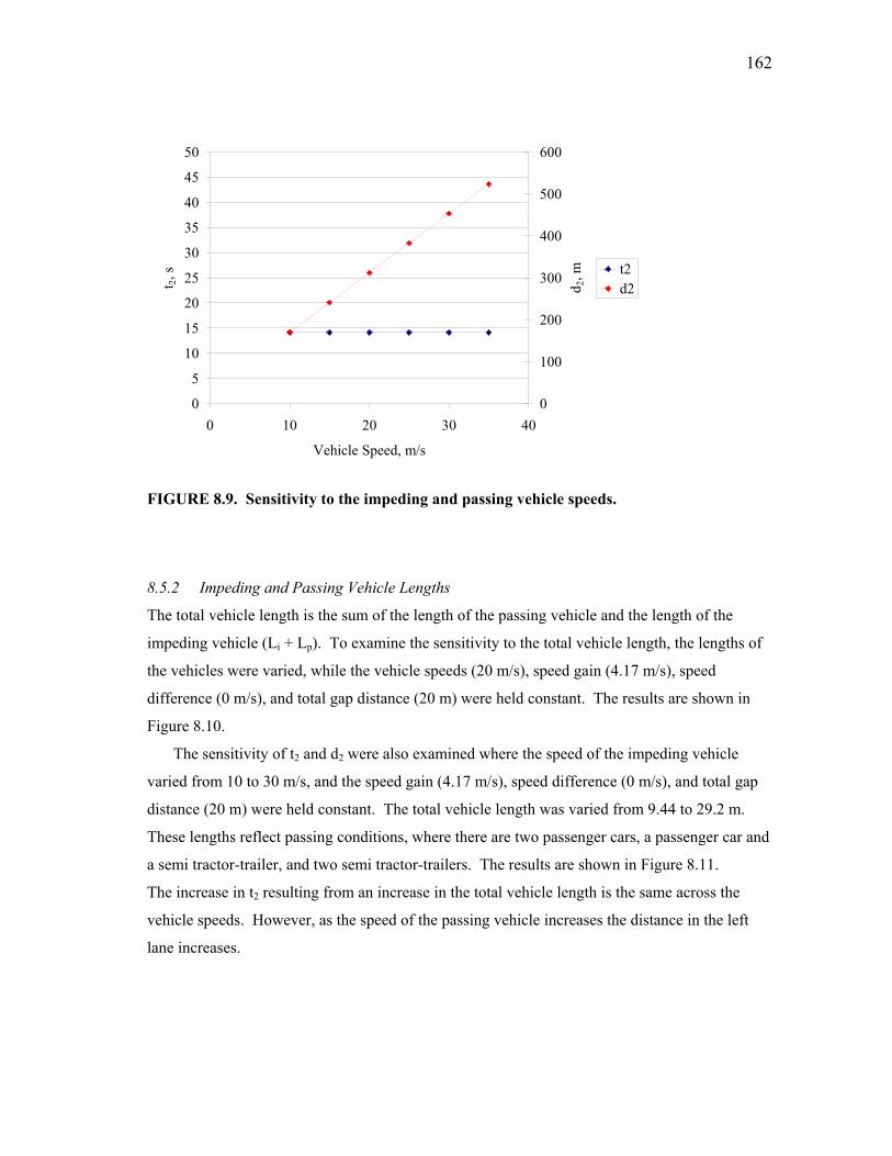
162
0
5
10
15
20
25
30
35
40
45
50
0 10 20 30 40
Vehicle Speed, m/s
t 2, s
0
100
200
300
400
500
600
d 2, m t2
d2
FIGURE 8.9. Sensitivity to the impeding and passing vehicle speeds.
8.5.2 Impeding and Passing Vehicle Lengths
The total vehicle length is the sum of the length of the passing vehicle and the length of the
impeding vehicle (Li + Lp). To examine the sensitivity to the total vehicle length, the lengths of
the vehicles were varied, while the vehicle speeds (20 m/s), speed gain (4.17 m/s), speed
difference (0 m/s), and total gap distance (20 m) were held constant. The results are shown in
Figure 8.10.
The sensitivity of t2 and d2 were also examined where the speed of the impeding vehicle
varied from 10 to 30 m/s, and the speed gain (4.17 m/s), speed difference (0 m/s), and total gap
distance (20 m) were held constant. The total vehicle length was varied from 9.44 to 29.2 m.
These lengths reflect passing conditions, where there are two passenger cars, a passenger car and
a semi tractor-trailer, and two semi tractor-trailers. The results are shown in Figure 8.11.
The increase in t2 resulting from an increase in the total vehicle length is the same across the
vehicle speeds. However, as the speed of the passing vehicle increases the distance in the left
lane increases.

163
0
5
10
15
20
25
30
35
40
45
50
0 10 20 30 40
Total Vehicle Length. m
t 2, s
0
100
200
300
400
500
600
d 2, m t2
d2
FIGURE 8.10. Sensitivity to the total vehicle length.
05
101520253035404550
0 10 20 30 40
Vehicle Speed, m/s
t 2, s
01002003004005006007008009001000
d 2, m
t2 (9.44 m)t2 (19.32 m)t2 (29.2 m)d2 (9.44 m)d2 (19.32 m)d2 (29.2 m)
FIGURE 8.11. Sensitivity to the impeding and passing vehicle lengths and speeds.

164
8.5.3 Gap Distances
The total gap distance is the sum of the start gap and end gap distances (GS+GE) that the passing
driver chooses to leave between the passing vehicle and the impeding vehicle. To examine the
sensitivity of t2 and d2, the total gap distances were varied, while the vehicle speeds (20 m/s),
speed gain (4.17 m/s), speed difference (0 m/s), and total vehicle length (9.44 m) were held
constant. The total gap distance was varied from 20 to 40 m. The results are shown in Figure
8.12.
The differences in t2 and d2 in response to changes the total gap distance are identical to the
differences in response to changes in the total vehicle length. This is because whether the total
vehicle length or the total gap distance increases, the result is an increase to the space
interchange and therefore an increase in t2 and d2. For a unit increase in the total gap distance, t2
increases by the reciprocal of the difference in the average speeds of the impeding and passing
vehicles ( ( 1ip ss −− ) ), and d2 increases by the change in the total gap distance plus the product
of the impeding vehicle speed and the time in the left lane ( ( ) 2i tsG∆ +∑ ).
0
5
10
15
20
25
30
35
40
45
50
0 10 20 30 40 50
Total Gap Distance, m
t 2, s
0
100
200
300
400
500
600
d 2, m t2
d2
FIGURE 8.12. Sensitivity to the total gap distance.
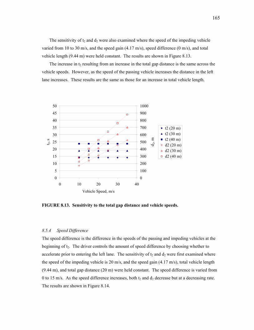
165
The sensitivity of t2 and d2 were also examined where the speed of the impeding vehicle
varied from 10 to 30 m/s, and the speed gain (4.17 m/s), speed difference (0 m/s), and total
vehicle length (9.44 m) were held constant. The results are shown in Figure 8.13.
The increase in t2 resulting from an increase in the total gap distance is the same across the
vehicle speeds. However, as the speed of the passing vehicle increases the distance in the left
lane increases. These results are the same as those for an increase in total vehicle length.
0
5
10
15
20
25
30
35
40
45
50
0 10 20 30 40
Vehicle Speed, m/s
t 2, s
0
100
200
300
400
500
600
700
800
900
1000
d 2, m
t2 (20 m)t2 (30 m)t2 (40 m)d2 (20 m)d2 (30 m)d2 (40 m)
FIGURE 8.13. Sensitivity to the total gap distance and vehicle speeds.
8.5.4 Speed Difference
The speed difference is the difference in the speeds of the passing and impeding vehicles at the
beginning of t2. The driver controls the amount of speed difference by choosing whether to
accelerate prior to entering the left lane. The sensitivity of t2 and d2 were first examined where
the speed of the impeding vehicle is 20 m/s, and the speed gain (4.17 m/s), total vehicle length
(9.44 m), and total gap distance (20 m) were held constant. The speed difference is varied from
0 to 15 m/s. As the speed difference increases, both t2 and d2 decrease but at a decreasing rate.
The results are shown in Figure 8.14.

166
As the speed difference increases, the rate at which the passing vehicle makes up the needed
distance also increases. Because t2 is inversely proportional to the rate the needed distance is
gained, t2 decreases at a decreasing rate. Thus, the passing vehicle spends less time and therefore
travels less distance in the left lane.
The sensitivity of t2 and d2 were also examined where the speed of the impeding vehicle
varied from 10 to 30 m/s, and the speed gain (4.17 m/s), total vehicle length (9.44 m), and total
gap distance (20 m) were held constant. The speed difference was varied from 0 to 10 m/s. The
sensitivity of t2 is the same across vehicle speeds but the sensitivity of d2 increases with higher
vehicle speeds. The results are shown in Figure 8.15.
The change in t2 for all impeding vehicle speeds is the result of the change in the rate that the
distance needed is gained. This relationship was illustrated in Figure 8.14 and occurs for all
impeding vehicle speeds in Figure 8.15. The decrease in d2 is larger for higher impeding vehicle
speeds because d2 is proportional to the product of the impeding vehicle speed and t2.
0
5
10
15
20
25
30
35
40
45
50
0 5 10 15
Speed Difference, m/s
t 2, s
0
50
100
150
200
250
300
350d 2
, m t2d2
FIGURE 8.14. Sensitivity to the speed difference.

167
0
5
10
15
20
25
30
35
40
45
50
0 10 20 30 40
Impeding Vehicle Speed, m/s
t 2, s
0
50
100
150
200
250
300
350
400
450
500
d 2, m
t2 (0 m/s)t2 (5 m/s)t2 (10 m/s)d2 (0 m/s)d2 (5 m/s)d2 (10 m/s)
FIGURE 8.15. Sensitivity to the speed difference and impeding vehicle speed.
8.5.5 Speed Gain
The speed gain, which is controlled by the passing driver, is the difference in the speed of the
passing vehicle during the time interval t2. To examine the sensitivity of t2 and d2, the speed gain
was varied, while the vehicle speeds (20 m/s), speed difference (0 m/s), total vehicle length (9.44
m), and total gap distance (20 m) were held constant. The speed gain was varied from 2 to10
m/s. The results are shown in Figure 8.16.
As the speed gain increases, the rate at which the passing vehicle makes up the needed
distance also increases. Thus, the passing vehicle spends less time and therefore travels less
distance in the left lane. Because t2 is inversely proportional to the rate the needed distance is
gained, t2 decreases at a decreasing rate.
The sensitivity of t2 and d2 was also examined where the speed of the impeding vehicle
varied from 10 to 30 m/s, and the speed difference (0 m/s), total vehicle length (9.44 m), and
total gap distance (20 m) were held constant. The speed gain was varied from 2 to 10 m/s. The
results are shown in Figure 8.17.

168
0
5
10
15
20
25
30
35
40
45
50
0 2 4 6 8 10 12
Speed Gain, m/s
t 2, s
0
100
200
300
400
500
600
700
d 2, m t2
d2
FIGURE 8.16. Sensitivity to the speed gain.
05
101520253035404550
0 10 20 30 40
Vehicle Speed, m/s
t 2, s
0
200
400
600
800
1000
1200
d 2, m
t2 (2.1 m/s)t2 (4.2 m/s)t2 (8.3 m/s)d2 (2.1 m/s)d2 (4.2 m/s)d2 (8.3 m/s)
FIGURE 8.17. Sensitivity to the speed gain and vehicle speeds.

169
The change in t2 for all impeding vehicle speeds is the result of the change in the rate that the
distance needed is gained. This relationship was illustrated in Figure 8.16 and occurs for all
impeding vehicle speeds in Figure 8.17. The decrease in d2 is larger for higher impeding vehicle
speeds because d2 is proportional to the product of the impeding vehicle speed and t2.
The differences in t2 and d2 in response to the speed gain are similar to the differences in
response to changes in the speed difference. Both the speed difference and speed gain contribute
to the rate at which the passing vehicle gains the needed distance. To produce the same response
in d2 and t2, the speed gain would need to be twice the change in the speed difference.
8.5.6 Summary
The passing distance is highly variable. In the passing equation, there are variables that reflect
the mechanics of the passing maneuver and variables that reflect passing behavior. Increases in
the speeds of the vehicles result in increases in d1, d2 and d4. Increases to the total vehicle length
or total gap length result in increases to t2 and d2. The driver can compensate for the increases in
d2 by increasing the speed difference at the beginning of t2 or the speed gain during t2. Of course
an increase in speed difference is also an increase in the speed of the passing vehicle during t1
and results in an increase in d1. The impact of the increase in the individual variable values on t2,
d1, d2, and d4 are summarized in Table 8.3.
TABLE 8.3. Summary of Responses to Increases in Model Variables
Response in passing maneuver Variable increased t2 d1 d2 d4
Vehicle speeds Total vehicle length Total gap distance Speed difference
Speed gain
It should be noted that the clearance distance, d3 is not included in the sensitivity analysis.
This distance is the result of the difference between the gap that is chosen in the opposing traffic
and some portion of the sum of d1, d2 and d4. The portion depends on when the acceptance of the
gap occurs. It may be argued that the gap is accepted at the beginning of t1, when the driver
perceives the opportunity to pass and begins the actions to execute the maneuver. Alternatively,

170
it could be argued that the gap is reassessed during the maneuver, and the gap is accepted
sometime during t2.
8.6 Predicting the Impact of Increasing the Impeding Vehicle Length
Through the sensitivity analysis, an increase in the total vehicle length was shown to positively
impact both the time and distance the passing vehicle travels in the left lane. The increase in t2 is
equal to the distance to be gained during the maneuver divided by the rate at which the passing
vehicle gains that distance.
gained is distance rategained be todistancet 2 = (8.15)
The rate can be represented as the difference in the average speeds of the impeding and passing
vehicles. The increase in t2 is then multiplied by the speed of the impeding vehicle and added to
the increase in the length of the impeding vehicle to determine the impact on d2. The increase in
d2 represents the change in the mechanics of the passing maneuver.
The relationship between the gain rate and d2 for total vehicle lengths of 9.4, 19.3, and 29.2
m is shown in Figure 8.18. These total vehicle lengths represent the passing conditions where
there are two passenger cars, a passenger car and a semi tractor-trailer, and two semi tractor-
trailers.
Increasing the gain rate decreases the distance the passing vehicle travels in the left lane.
The passing driver can increase speed, thereby increasing the gain rate to compensate for the
added distance to be gained caused by an in crease in the total vehicle length. For instance, at a
gain rate of 3 m/s, a passing passenger car travels approximately 240 meters in the left lane to
overtake another passenger car. If the impeding vehicle is a semi tractor-trailer, a passing
passenger car can still overtake the impeding vehicle in the same distance if the gain rate is
increased to 5 m/s. If both vehicles are semi tractor-trailers, the gain rate needs to be increased
to 6 m/s for the passing vehicle to overtake the impeding vehicle in the same distance.
An increase in the gain rate may be achieved in two ways: by increasing the speed difference
by accelerating during t1 or by increasing the speed gained during t2. Either way will help to
compensate for the impact of an increase to the total vehicle length on the distance and time in
the left lane. However, if the driver increases speed during t1, there is also an increase in d1 and
the total passing distance (D).

171
0
5
10
15
20
25
30
35
40
45
50
0 2 4 6 8
Gain Rate, m/s
t 2, s
0
100
200
300
400
500
600
d 2, m
t2 (9.4 m)t2 (19.3 m)t2 (29.2 m)d2 (9.4 m)d2 (19.3 m)d2 (29.2 m)
FIGURE 8.18. Sensitivity to gain rate and vehicle lengths.
0
5
10
15
20
25
30
35
40
45
50
40 60 80 100
Average Speed of Passing Vehicle, km/h
t 2, s
0
50
100
150
200
250
300
350
400
450
500
d 2, m
t2 (calibrated)t2 (+5 m)t2 (+10 m)t2 (+15 m)t2 (+20 m)d2 (calibrated)d2 (+5 m)d2 (+10 m)d2 (+15 m)d2 (+20 m)
FIGURE 8.19. Predicted impact of vehicle length on AASHTO design values.

172
An important consideration is that the increase in the gain rate is limited by the performance
of the passing vehicle under the specific passing conditions. Vehicles with poor acceleration
capabilities may not be able to achieve the higher gain rates. Steep grades may also prevent
vehicles from achieving a high gain rate. In addition, some drivers may not be comfortable with
large gain rates, especially if the speed limit is exceeded. Therefore, compensating for the
impact of the increase in the total vehicle length on the time and distance in the left lane is
dependent on vehicle, environment, and driver factors.
Using the passing model, calibrated for the ASSHTO design variables, the increase in the
length of the impeding vehicle was examined. The predicted increase in d2, shown in Figure
8.19, represents changes only in the mechanics of the passing maneuver and not changes in
passing behavior.
Under the passing conditions described by the ASSHTO design values, a one meter increase
in the total vehicle length is predicted to cause an increase in t2 of 0.24 seconds. This impact is
the same regardless of the average speed of the passing vehicle. However, the impact on d2
depends on the average speed of the impeding vehicle. The marginal changes in t2 and d2 are
summarized in Table 8.4.
TABLE 8.4. Marginal Changes in t2 and d2 for Total Vehicle Length.
Average passing vehicle speed, km/h Marginal change in t2, s Marginal change in d2, m 56.2 0.24 3.74 70 0.24 4.67
84.5 0.24 5.64 99.8 0.24 6.66
The marginal differences only represent the changes in the mechanics of the passing
maneuver. It is possible that the passing driver may behave differently depending on the type of
impeding vehicle. Perhaps the length, width, type of cargo or some other characteristic about the
impeding vehicle is perceived in such a way that the passing driver leaves more space. An
increase in the total gap distance would also add to the space interchange thereby increasing the
time and distance traveled in the left lane. Polus et al. reported that the gap distances were larger
when the impeding vehicles were trucks or buses rather than passenger cars (22). If the behavior

173
observed in Israel is similar to the behavior in the United States of America, then the marginal
differences presented in Table 8.4 are underestimated.
8.6.1 Passing Sight Distance Design Practices
The current passing sight distance values are published in A Policy on Geometric Design of
Highways and Streets (10). The distances are shown in Table 3.1. They are based the passing
driver determining at the start of the passing maneuver that the opposing traffic lane is clear to
successfully complete a passing maneuver. The passing situation is a passenger car overtaking
another passenger car on a level roadway. It has been suggested that the increase in the vehicle
length would require greater passing distance. On unfavorable grades, such as steep inclines, it
is recommended that the passing sight distances should be increased.
The passing equations have been calibrated to the AASHTO values and include variables
that represent the mechanics of the passing maneuver and passing behavior that can be adjusted
to describe a variety of passing conditions. These equations are much more valuable than the
AASHTO representation of passing distances because they can be calibrated to a variety of
conditions and used to predict the impact to the passing distance given changes to the mechanics
of the passing maneuver. For instance, when large trucks are being considered as the impeding
vehicle, not only is the length of the vehicle a concern but also the performance of the vehicle. If
the passing maneuver occurs on a grade, an impeding truck may lose speed on a positive grade
or gain speed on a negative grade. This would change the average speed of the impeding vehicle
and could be incorporated into the equations to predict the impact of t2 and d2.
The passing equations can also be used to identify what changes in driver behavior are
needed to compensate for changes in factors that impact the mechanics of the passing maneuver.
Using the same example of a change in the grade and an impeding truck, on a positive grade the
speed gain needed by the passing vehicle would decrease whereas on the negative grade the
needed speed gain would increase. Depending on the performance of the passing vehicle and
other passing conditions, the larger speed gain may not be achievable.
8.6.2 No-Passing Zones Marking Practices
The current passing sight distance values for marking no-passing zones are published in the
Manual on Uniform Traffic Control Devices (12). The distances are shown in Table 3.3. The
passing sight distance values used for marking are less than those used in design. The
inconsistency between the passing sight distances for design and for marking are a concern

174
because there is a potential that a section of roadway designed with inadequate passing sight
distance may be marked for passing.
Glennon (17) suggested that a critical passing sight distance should be provided at the end of
every passing area. This distance is described as the passing sight distance needed at the critical
point or point of no return, which is the moment when the same sight distance is needed to abort
or complete the pass with the same amount of safety. The measure of the safety is the clearance
to the opposing vehicle at the end of the aborted or completed pass. To calculate the critical
passing sight distance, it is assumed that the driver can decide when the critical point or point of
no return has been reached. This is a complicated decision and given the difficulties of judging
distance, speed, time to collision, it is unlikely that drivers can accurately determine when the
critical point has been reached. Nonetheless, the notion that there should be a connection
between the passing sight distances for design and marking is credible. The exact relationship
between the passing sight distances for design and marking needs to be determined to ensure that
the passing and no-passing areas operate as the roadway was designed.
Under the current marking practices, the minimum passing sight distance is available at any
point within the passing area. The worse case scenario is that the passing maneuver has not been
completed when the end of the passing area is reached. If it is assumed the passing and opposing
vehicles are traveling at the speed limit during the passing maneuver, and the opposing vehicle
enters the line of sight, the minimum passing sight distances are equivalent to approximately a
five second time to collision. To ensure a one second clearance at the end of the maneuver, the
pass needs to be completed or aborted within about four seconds. In most states, the driver is not
allowed to drive left of a solid, yellow centerline therefore, the pass must be completed prior to
the end of the passing area. What limits the size of the passing area is a minimum allowable
distance of 120 m between no-passing areas. In practice, some engineers find it prudent to
increase this minimum allowable distance (126), which is reasonable because a passing
maneuver cannot be performed in a 120 m section of highway. Perhaps the minimum allowable
distance should be the same as the minimum sight distance, however there still needs to be some
link to the passing sight distance used for design.
Once the relationship between the passing sight distances for design and marking is
established, the passing equation could be adjusted to produce a passing model for marking that
is sensitive to changes in the passing conditions. Changes to factors that impact the mechanics
of the maneuver and passing behavior could then be incorporated into the marking practices. For

175
instance, maybe longer minimum passing sections are needed on positive grades and in areas
where there are a large percentage of trucks. Compared to a level roadway with only passenger
cars as impeding and passing vehicles, these types of passing conditions require greater passing
distances; therefore providing a longer minimum passing area would be prudent.
8.7 Evaluating Passing Behavior
In the field, it is difficult to track both the passing and impeding vehicle with enough accuracy so
as to obtain the speed profiles of the vehicles over the duration of the maneuver. With the
passing equation, the speed of the passing vehicle at the beginning and end of the maneuver can
be used in combination with the observed time and distance in the left lane to describe what type
of passing maneuver was performed. The average speed observed in the field is calculated as
( )2
2p t
dobserveds = (8.16)
The estimated average speed, as considered in the passing equation, is calculated as
( )2∆s
spredicteds ppp += (8.17)
If the observed and estimated average speeds of the passing vehicle are equal, then the passing
vehicle increased speed linearly over the time interval t2. In other words the acceleration was
constant over t2. If during t2, the acceleration decreased, the observed average speed would be
greater than the estimated average speed. Similarly, if during t2 the acceleration increased, the
observed average speed would be less than the estimated average speed.
Using this relationship, and the assumption that the acceleration behavior represents the
perceived threat of the opposing vehicle, confidence in completing the pass, and opportunity to
move back into the right lane, some comments can be made about the type of passing maneuver
being observed.
In the situation where the observed average speed is greater than the estimated average
speed, the driver was more aggressive in the beginning of the pass and less aggressive at the end
of the pass. This behavior suggests that the driver had confidence that the pass could be
completed and perceived the threat of the opposing vehicle to be low and therefore, decreased
acceleration. In the situation where the observed average speed is less than the estimated

176
average speed, the driver was less aggressive during the beginning of the pass and more
aggressive during the end of the pass. This behavior suggests that sometime during the pass the
driver’s perception of the threat of the opposing vehicle increased given the percentage of the
pass that has been completed or that the opportunity to return to the right lane was challenged.
The driver responded by increasing acceleration to ensure the pass was completed successfully.
This type of evaluation could be beneficial for identifying problem areas for passing. If a
consistent passing behavior is observed, it may indicate a problem inherent in the specific
location. For instance, if drivers are consistently increasing acceleration late in the pass, this
behavior may indicate that the sight distance is inadequate and drivers are not seeing an
opposing vehicle until well into the pass. It could also indicate that a driveway or other potential
conflict is present that is not seen until late into the maneuver. The results of such an
investigation might support the need for additional signage for hidden driveways or perhaps a
change in the passing markings.

177
9 SUMMARY
The methodology, presented as a general framework for improving simulations through
distributed computing, was used to create a prototype. The methodology was motivated by the
need to capture behavior in traffic simulations and the need to create specific traffic flows in
driving simulations. The prototype was designed based on HLA and the RTI was to facilitate the
two-way real-time communication between a VISSIM simulation and a comparable DriveSafety
simulation.
Problems were encountered, which constrained the development of the prototype and its
usefulness. The major problems included:
1. Queuing during the export of data from VISSIM;
2. Queuing of data in the translator program; and
3. A processing threshold of thirty vehicle speed updates per second in DriveSafety.
With delays in the transfer of data, a two-way real-time data transfer was not feasible. These
problems will need to be solved before the prototype can be further developed. The translator
program will need to be rewritten as a multithread application, which will allow simultaneous
read and write capabilities. The processing threshold in DriveSafety, which limited the update
rate, number of vehicles, and therefore the traffic volume and size of the network being
simulated, will need to be addressed. If this threshold is not remedied, the usefulness of
prototypes such as the one developed for this research cannot be fully explored.
In the final prototype, vehicle information from VISSIM was transferred to DriveSafety to
generate vehicles and control their speed during the simulation. This prototype was successfully
applied to a passing study, where the impact of the length of the impeding vehicle on passing
behavior was investigated. Using the data from VISSIM, two platoons of impeding vehicles
were generated in DriveSafety and their speeds were controlled for the duration of the
simulation. An opposing traffic flow of 250 vehicles per hour was also generated and controlled
in the same manner. Details about the movement of the test vehicle, controlled by the test driver,
were recorded directly in the DriveSafety data collection file. Details about the movement of the
impeding and opposing vehicles were estimated by comparing the data from the VISSIM data

178
collection file, and the log of trigger activations in DriveSafety. Had a two-way real-time data
exchange been achieved, the traffic data could have been read directly from the VISSIM data
collection file.
The passing study was designed as a repeated measure, 2x2 factorial, where the impeding
vehicles differed by length and by speed. The length on the impeding vehicle was found to
significantly impact the time and distance in the left lane as well as the start gap and end gap
distances. These results support the notion that the impact was not limited to the additional
length of the impeding vehicle that the passing vehicle needed to gain during the maneuver. The
impact was also a result of changes in the behavior of the passing driver, as indicated by the
difference in gap distances.
The variation in passing behavior was further explored by examining the data collected
during the passing study. The variations in start gap and end gap distances, speed gain, speed
difference, maximum speed, and acceleration behavior was examined. The variation in the types
of passing maneuvers was also examined. A relationship between the speed difference and
speed gain was identified and can be used to describe the start of the pass. A relationship
between the location of the passing vehicle with respect to the impeding vehicle and the
clearance distance at the time the passing vehicle first decelerates was also identified. This
relationship can be used to describe the end of the pass and perhaps also describe how the
passing driver perceives the threat of the opposing vehicle in terms of the successful completion
of the pass. This relationship may be more complex, and need to account for the opportunity to
return to the right lane.
Using some of the insight gained during the passing study and the subsequent examination
of the passing data, a series of passing equations were developed to describe the four elements of
the passing maneuver. The equations were brought together to form the following equation
describing the total passing distance.
( )21oEp2iiS1p ttsCGLtsLGtsD ++++++++= (9.1)
The variables that reflect the mechanics of the passing maneuver include the speeds and lengths
of the vehicles. The variables that reflect passing behavior include the gap distances and speed
gain of the passing vehicle used to calculate t2. The sensitivity of t2 and d2 to these variables was
examined. Increases to the vehicle length and gap distances increased t2 and increases in the

179
speed difference and speed gain decreased t2. Increases in the vehicle speeds, vehicle lengths,
and gap distances increased d2, and increases in the speed difference and speed gain decreased
d2.
The equations for t2 and d2 were validated using the data from the passing study and
calibrated using the AASHTO passing sight distance criteria. The calibrated equations were
used to predict the impact of longer impeding vehicles. With a one meter increase in the length
of the impeding vehicle, the marginal increase in t2 was 0.24 seconds and the marginal increase
in d2 was 3.74 meters at an average passing vehicle speed of 56.2 km/h and 6.66 meters at an
average passing vehicle speed of 99.8 km/h.
9.1 Contributions
The contributions of this research derive from the two focus areas: the development of a
methodology to combine microscopic traffic simulation programs with driving simulator
programs, and the application of a prototype distributed traffic simulation to study the impact of
the length of an impeding vehicle on passing behavior.
9.1.1 Methodology
Although distributed simulation is not a new idea, it has failed to receive much attention in the
area of transportation, especially in the civil domain. Some efforts in Europe, specifically in
Germany and the Netherlands, have been reported but this research appears to be the first
reported in the United States.
Since the methodology was generic in nature, it could be used to develop a variety of
distributed simulations for a variety of traffic or behavior problems. In fact, a distributed
simulation comprised of two contributing simulations could be expanded upon to incorporate
multiple simulations, or other applications. Ultimately, a distributed simulation could be
developed as an open traffic environment linking together an assortment of traffic simulations,
databases, data acquisition tools, analyses programs, and visualization tools.
This methodology should be attractive to the users of traffic simulation because it increases
the number of tools available for traffic and behavior analysis. It should also be attractive to
developers because this is one avenue to increase the life and usefulness of their products and at
the same time it provides the opportunity to create very specific programs that can be
incorporated into larger simulations.

180
A distributed simulation, combining a traffic simulation and a driving simulation, is a good
data collection tool. The laboratory setting is a safe and easily controlled environment and
provides direct contact with the test drivers. A lot of data can be captured about the test driver,
vehicle, and environment. Similar access to the test driver is not available in field studies and if
it is even possible to capture very detailed data about the vehicle and environment, the methods
are likely quite costly, difficult, and dangerous to implement.
9.1.2 Application
Historically, the passing maneuver has been studied by making observations in the field,
conducting experiments in the field, or conducting experiments on closed courses. This is the
first reported study in the United States to investigate passing behavior in a simulated
environment.
The motivation behind using the prototype to study passing behavior was the potential that
federal truck size and weight regulations will change and the current inconsistency between the
passing sight distance criteria for designing two lane highways and marking no passing zones.
To ensure the safe operation of the two-lane two-way highways, it is necessary that the impact of
longer trucks be understood and considered in the design and marking of the highways. One of
the benefits of the simulated environment is the ability to simulate vehicles that do not exist.
Although it was not done for this research, vehicles longer than what is permitted under the
current federal regulations could be used to examine the impact of these long vehicles.
There are concerns about the validity of using the simulated environment and the potential
for test drivers to behave differently than they do in the real world. From the results of the
passing study and the comparison of the summarized data to field data reported by Polus et al.
(22), there is hope that simulated environments are suitable for passing studies and that the
results are transferable to the real world. The data summarized using the conventional definition
for the occupation of the left lane did not compare well to the field data, however, the data
summarized using the alternate definition was much better. In fact, it was found that the means
of the distance in the left lane from the simulated study and the field study were comparable.
9.1.3 Passing Equation
The passing equation has several uses. It can be used to evaluate the passing sight distance
criteria for design and marking no-passing zones. It can also be used to evaluate the passing
behavior observed in the field. By comparing the actual average speed of the passing vehicle to

181
the estimated average speed of the passing vehicle, calculated using the passing equation,
conclusions can be drawn about the acceleration of the passing vehicle. For example, if the
actual average speed is greater than the estimated, than the majority of the increase in speed
occurred during the beginning of the pass. This type of comparison requires only a few field
observations and could be used to identify problem areas for passing.
9.2 Future Research
This research was multidiscipline in nature and literature was drawn from simulation, distributed
computing, transportation, human factors, and psychology publication sources. It is not
surprising then, that the recommended future research extends over several areas.
9.2.1 Distributed Computing
The first recommendation is to continue the efforts to advance the field of distributed computing.
This recommendation is obvious considering computer technology, web technology, and
networking technology are areas of strong investment. A good source for the current research is
the journal Simulation: Transactions of The Society for Modeling and Simulation International.
The story behind the High Level Architecture is a good example of the benefits of
distributed computing. Without the funding to create new simulations, and a vast library of old
simulations, HLA was developed as a framework to provide the reuse of simulations and the
interoperability among simulations. The old simulations became a new resource to be reused to
address new problems.
Distributed computing has been implemented in many industrial domains including
manufacturing, supply chains, and emergency planning. The experience in transportation is very
limited apart from the use of HLA for the simulation of military operations. This means that
there is a wealth of opportunity to examine the potential of distributing computing within the
field of transportation.
9.2.2 Simulation
The second recommendation is to examine the validity of transportation simulations and the
transferability of the study results to the real world. It is all too easy to use a simulation as a
black box but this approach can lead to erroneous interpretation of the simulation results. The
results of traffic and/or driving simulations reflect the logic incorporated into the models, the
assumptions and simplifications that were made, and the methods of introducing randomness. In

182
the case of a driving simulation, the captured behavior may be influenced by the characteristics
of the animation, interface, and testing environment. The test driver’s reaction to the driving
environment, in terms of the symptoms of simulator sickness, may also influence the behavior of
the driver. Research is needed to validate the host of different traffic and driving simulations.
9.2.3 Behavior Analysis
The third recommendation is to continue examining passing behavior and the impact of trucks
and other driver, vehicle and environment factors. Further detailed passing data is needed to
determine what type of response is expected under a variety of passing conditions. Additional
data is also needed to verify the continuum between the flying and accelerated starts as well as
the continuum between the voluntary and forced returns. One interesting area will be to
determine how the opportunity to return to the right lane needs to be incorporated into the
relationship describing the end of the passing maneuver.
The fourth recommendation is to enhance the deterministic passing equation to reflect the
dynamic and stochastic behavior of drivers. This could be achieved by generating the values for
the behavior variables using a random number generator and the distributions for the response
variables observed during the passing study. It would then be possible to generate a sample of
passing distances and times that could be used to predict behavior or evaluate passing sight
distance criteria.
9.2.4 Traffic Analysis
The fifth recommendation is to define the relationship between the criteria for designing two
lane highways and marking no passing zones, and determine what passing conditions should be
reflected by those criteria. The current inconsistency in the criteria is concerning as sections of
roadway not designed for passing may be subsequently marked as passing areas. The safety
implications of this inconsistency are clear; the markings suggest to the driver that it is safe to
pass while the design of the road requires that the driver judge whether or not it is truly safe to
pass. These criteria could change dramatically depending upon whether the criteria are based on
a flying start and voluntary return pass, or an accelerated start and hurried return pass, or some
combination thereof. The final criteria will impact the capacity of two lane highways, as the
opportunity to pass may change. This in turn may change the passing behavior of drivers and
require further investigation into the interactions between passenger cars and trucks, and the
results should be incorporated into traffic simulations.

183
REFERENCES
1. Highway Capacity Manual. Transportation Research Board, National Research Council, Washington, DC, 2000.
2. Algers, S., E. Bernauer, M. Boero, L. Breheret, C. Di Taranto, M. Dougherty, K. Fox, and J. F. Gabard. Simulation Modeling Applied to Road Transport European Scheme Tests: Review of Micro-simulation Models. Institute for Transport Studies, University of Leeds, Leeds, 1997. http://www.its.leeds.ac.uk/projects/smartest/, Accessed April 2004.
3. Institut National de Recherche sur les Transports et leur Securite. Driving Simulators Links. Updated March 31, 2004, http://www.inrets.fr/ur/sara/Pg_simus_e.html, Accessed April 2004.
4. Greenshields, B. D. Distance and Time Required to Overtake and Pass Cars. In Highway Research Board Proceedings, Vol. 15, 1935, pp. 332-341.
5. Matson, T. M., and T. W. Forbes. Overtaking and Passing Requirements as Determined from a Moving Vehicle. In Highway Research Board Proceedings, Vol. 18, Pt. 1, 1938, pp. 100-112.
6. Forbes, T. W., and T. M. Matson. Driver Judgments in Passing on the Highway. The Journal of Psychology, Vol. 8, 1939, pp. 3-11.
7. Forbes, T. W. Methods of Measuring Judgment and Perception Time in Passing on the Highway. In Highway Research Board Proceedings, Vol. 19, 1939, pp. 218-231.
8. Holmes, E. H. Procedure Employed in Analysis of Passing Distances. In Highway Research Board Proceedings, Vol. 18, Pt. 1, 1938, pp. 368-370.
9. Prisk, C. W. Passing Practices on Rural Highways. In Highway Research Board Proceedings, Vol. 21, 1941, pp. 366-378.
10. A Policy on Geometric Design of Highways and Streets. American Association of State Highway and Transportation Officials, Washington, DC, 2001.
11. A Policy on Geometric Design of Highways and Streets. American Association of State Highway and Transportation Officials, Washington, DC, 1994.
12. Manual on Uniform Traffic Control Devices, Part 3, Markings. Federal Highway Administration. Washington, DC, 2001.
13. A Policy of Marking and Signing of No-Passing Zones on Two- and Three-Lane Roads. American Association of State Highway Officials, Washington, DC, 1940.
14. Herman, R., and T. Lam. A Dilemma in Overtaking on Two-Lane Roads. Traffic Engineering and Control, Vol. 14, 1972, pp. 276-279, 289.
15. Lieberman, E. B. Model for Calculating Safe Passing Distances on Two-Lane Rural Roads. In Transportation Research Record: Journal of the Transportation Research Board, No. 869, TRB, National Research Council, Washington, DC, 1982, pp. 70-76.

184
16. Saito, M. Evaluation of the Adequacy of the MUTCD Minimum Passing Sight Distance Requirement for Aborting the Passing Maneuver. Institute of Transportation Engineers Journal, Vol. 54, No. 1, 1984, pp. 18-22.
17. Glennon, J. C. New and Improved Model of Passing Sight Distance on Two-Lane Highways. In Transportation Research Record: Journal of the Transportation Research Board, No. 1195, TRB, National Research Council, Washington, DC, 1988, pp. 132-137.
18. Rilett, L. R., B. G. Hutchinson, and M. Whitney. Mechanics of the Passing Maneuver and the Impact of Large Trucks. Transportation Research Part A: General, Vol. 24, No. 2, 1990, pp. 121-128.
19. Hassan, Y., S. M. Easa, and A. O. Abd El Halim. Passing Sight Distance on Two-Lane Highways: Review and Revision. Transportation Research Part A: Policy and Practice, Vol. 30, No. 6, 1996, pp. 453-467.
20. Harwood, D. W., and J. C. Glennon. Passing Sight Distance Design for Passenger Cars and Trucks. In Transportation Research Record: Journal of the Transportation Research Board, No. 1208, TRB, National Research Council, Washington, DC, 1989, pp. 59-69.
21. Good, D., J. B. L. Robinson, G. Sparks, and R. Neudorf. The Effect of Vehicle Length on Traffic on Canadian Two-Lane, Two-Way Roads. Report No. CA6 ARH 91E 28. Transportation Association of Canada, 1991.
22. Polus, A., M. Livneh, and B. Frischer. Evaluation of the Passing Process on Two-Lane Rural Highways. In Transportation Research Record: Journal of the Transportation Research Board, No. 1701, TRB, National Research Council, Washington, DC, 2000, pp. 53-60.
23. Nance, R. E. Distributed Simulation with Federated Models: Expectations, Realizations and Limitations. In Proceedings of the 1999 Winter Simulation Conference, Eds. Farrington, P. A., H. B. Nembhard, D. T. Sturrock, and G. W. Evans. 1999, pp. 1026-1031.
24. VISSIM User Manual – Version 3.60. Planung Transport Verkehr AG. Stumpfsrasse 1, D-76131 Karlsruhe, Germany, December 2001.
25. HyperDrive Version 1.5.2. User Manual. GlobalSim Inc. 12159 S. Business Park Drive, Salt Lake City, UT, 2002.
26. Klein, U., T. Schulze, S. Strassburger and H.-P. Menzler. Traffic Simulation Based on the High Level Architecture. In Proceedings of the 1998 Winter Simulation Conference, Eds. Medeiros, D. J., E.F. Watson, J.S. Carson, and M.S. Manivannan, 1998, pp. 1095-1103.
27. Klein, U., T. Schulze, S. Straßburger and H.-P. Menzler. Distributed Traffic Simulation Based on the High Level Architecture. In Proceedings of the 1998 Fall Simulation Interoperability Workshop, September 1999, Orlando, FL, USA.
28. Pipes, L. A. An Operational Analysis of Traffic Dynamics. Journal of Applied Physics, Vol. 24, No. 3, 1953, pp. 274-281.

185
29. Forbes, T. W., H. J. Zagorski, E. L. Holshouser, and W. A Deterline. Measurement of Driver Reaction to Tunnel Conditions, In Highway Research Board Proceedings, Vol. 37, 1958, pp. 345-357.
30. Forbes, T. W. Human Factor Considerations in Traffic Flow Theory. In Highway Research Record, No. 15, Highway Research Board, Washington DC, 1963, pp. 60-66.
31. Forbes, T. W., and M. E. Simpson. Driver and Vehicle Response in Freeway Deceleration Waves. Transportation Science, Vol. 2, No. 1, 1968, pp. 77-104.
32. May, A. D. Traffic Flow Fundamentals. Prentice Hall, Engelwood Cliffs, NJ, 1990.
33. Chandler, R.E., R. Herman, and E.W. Montroll. Traffic Dynamics: Studies in Car Following. Operations Research: The Journal of the Operations Research Society of America, Vol. 6, No. 2, 1958, pp. 165-184.
34. Herman, R., E. W. Montroll, R. B. Potts, and R. W. Rothery. Traffic Dynamics: Analysis of Stability in Car Following. Operations Research: The Journal of the Operations Research Society of America, Vol. 7, No. 1, 1959, pp 86-106.
35. Gazis, D. C., R. Herman, and R. B. Potts. Car-Following Theory of Steady-State Traffic Flow. Operations Research: The Journal of the Operations Research Society of America, Vol. 7, No. 4, 1959, pp. 499-505.
36. Gazis, D. C, R. Herman, and R. W. Rothery. Nonlinear Follow-the-Leader Models of Traffic Flow. Operations Research: The Journal of the Operations Research Society of America, Vol. 9, No. 4, 1961, pp. 545-567.
37. Brackstone, M., and M. McDonald. Car-following: a Historical Review. In Transportation Research Part F: Traffic Psychology and Behavior, Vol. 2, No. 4, 1999, pp. 181-196.
38. Newell, G. F. Theory of Highway Traffic Flow 1945-1965, Course Notes UCB-ITS-CN-95-1, Institute of Transportation Studies, University of California, Berkley, CA, 1995.
39. Revised Monograph on Traffic Flow Theory. Eds. Gartner, N. H., C. J. Messer, and A. K. Rathi. Transportation Research Board, National Research Council, Washington, DC, November 1997.
40. D. L. Gerlough and M. J. Huber. Traffic Flow Theory. Special Report No. 165. Transportation Research Board, National Research Council, Washington, DC, 1975.
41. E. W. Montroll and R. B. Potts. Car Following and Acceleration Noise. In An Introduction to Traffic Flow Theory, Special Report 79, Highway Research Board, National Research Council, Washington, DC, 1964, pp. 37-48.
42. Greenberg, H. An Analysis of Traffic Flow. Operation Research: The Journal of the Operations Research Society of America, Vol. 7, 1959, pp. 79-85.
43. Drew, D. R. Deterministic Aspects of Freeway Operations and Control. Research Report 24-4. Texas Transportation Institute, Texas A&M University, College Station, TX, June 1965.
44. Greenshields, B. D. A Study in Highway Capacity. In Highway Research Board Proceedings, Vol. 14, 1934, pp. 468.

186
45. Edie, L. C. Car-Following and Steady-State Theory for Noncongested Traffic. Operations Research: The Journal of the Operations Research Society of America, Vol. 9, No. 1, 1961, pp. 66-76.
46. Underwood, R. T. Speed, Volume, and Density Relationships. Quality and Theory of Traffic Flow. Yale Bureau of Highway Traffic, 1961, pp. 141-188.
47. May, A. D. Jr., and H. E. M. Keller. Non-Integer Car-Following Models. Highway Research Record, No. 199, Highway Research Board, National Research Council, Washington, DC, 1967, pp. 19-32.
48. Aycin, M. F., and R. F. Benekohal. Comparison of Car-Following Models for Simulation. In Transportation Research Record: Journal of the Transportation Research Board, No. 1678, TRB, National Research Council, Washington, DC, 1999, pp. 116-127.
49. Halati, A., H. Lieu, and S. Walker. CORSIM Corridor Traffic Simulation Model. In Traffic Congestion and Traffic Safety in the 21st Century: Challenges, Innovations, and Opportunities. Ed. R. F. Benekohal. American Society of Civil Engineers. 1997, pp. 570-576.
50. Halati, A., H. Lieu, and S. Walker. CORSIM–Corridor Traffic Simulation Model, Prepared for Transportation Research Board 76th Annual Meeting, Washington, DC, January 1997.
51. Rakha, H., and B. Crowther. Comparison of Greenshields, Pipes, and Van Aerde Car-Following and Traffic Stream Models. In Transportation Research Record: Journal of the Transportation Research Board, No 1802, TRB, National Research Council, Washington, DC, 2002, pp. 248-262.
52. Rakha, H., and B. Crowther. Comparison and Calibration of FRESIM and INTEGRATION Steady-State Car-Following Behavior. In Transportation Research Part A: Policy and Practice, Vol. 37, No. 1, 2003, pp. 1-27.
53. Gipps, P. G. A Behavioural Car-Following Model for Computer Simulation. In Transportation Research Part B: Methodological, Vol. 15, No. 2, 1981, pp 105-111.
54. Young, W., M. A. P. Taylor, and P. G. Gipps. Microcomputers in Traffic Engineering. John Wiley & Sons Inc. New York, NY, 1989.
55. Gipps, P.G. MULTSIM: A Model for Simulating Vehicular Traffic on Multi-Lane Arterial Roads. Mathematics and Computers in Simulation, Vol. 28, 1986, pp. 291-295.
56. Michaels, R. M. Perceptual factors in car following. In Proceedings of the Second International Symposium on the Theory of Traffic Flow, Ed. Almond, J., Paris: OECD, 1965, pp. 44-59.
57. Todosiev, E. P. The Actionpoint Model of Driver-Vehicle System. Engineering Experiment Station, The Ohio State University, Columbus, OH, Report 202 A-3, 1963.
58. Todosiev, E. P., and L. C. Barbosa. A Proposed Model for the Driver-Vehicle System. Traffic Engineering, Vol. 34, No. 17, 1964, pp. 17-20.
59. Goldstein, E. B. Sensation and Perception, Sixth Edition. Wadsworth, Pacific Grove, CA, 2002.

187
60. Gordon, D. A. The Driver in Single Lane Traffic. In Highway Research Record, No. 349, Highway Research Board, National Research Council, Washington, DC, 1971, pp. 31-40.
61. Brackstone, M., B. Sultan, and M. McDonald. Motorway Driver Behaviour: Studies on Car Following. Transportation Research Part F: Traffic Psychology and Behaviour, Vol. 5, No. 1, 2002, pp. 31-46.
62. Evans, L., and R. Rothery. Experimental Measurement of Perceptual Thresholds in Car Following. In Highway Research Record, No 64, Highway Research Board, National Research Council, Washington, DC, 1973, pp. 13-29.
63. Evans, L., and R. Rothery. Perceptual Thresholds in Car Following – A Recent Comparison. Transportation Science, Vol. 11, No. 1, 1977, pp. 60-72.
64. Leutzbach, W., and R. Wiedemann. Development and Applications of Traffic Simulation Models at the Karlsruhe Institut für Verkehrwesen. Traffic Engineering and Control, Vol. 25, No. 5, 1986, pp 270-278.
65. Reiter, U. Empirical Studies as a Basis for Traffic Flow Models. In Proceedings of the Second International Symposium on Highway Capacity, Vol. 2, 1994, pp. 493-502.
66. Wiedemann, R., and U. Reiter. Microscopic Traffic Simulation: The Simulation System MISSION. http://www.itc-world.com/docs/ Accessed April 2004.
67. Wiedemann, R., Modelling of RTI-Elements on Multi-Lane Roads. In Advanced Telematics in Road Transport, Proceedings of the DRIVE Conference, Vol. 2, Brussels, Belgium, February 4-6, 1991, pp. 1007-1019.
68. Ehmanns, D., and A. Hochstädter. Driver-Model Of Lane Change Maneuvers. 7th World Congress on Intelligent Transport Systems, Turin, Italy, November 2000.
69. Fritzsche, H. T. A Model for Traffic Simulation. Traffic Engineering and Control, Vol. 35, No. 5, 1994, pp. 317-321.
70. Lee, J., and J.H. Jones. Traffic Dynamics: Visual Angle Car Following Models. Traffic Engineering and Control, Vol. 9, No. 7, 1967, pp. 348-350.
71. Gipps, P. G. A Model for the Structure of Lane-Changing Decisions. Transportation Research Part B: Methodological, Vol. 20, No. 5, 1986, pp. 403-414.
72. Gipps, P. G., and B. G. Wilson. MULTSIM: A Computer Package for Simulating Multi-Lane Traffic Flows. In Proceedings of the Fourth Biennial Conference, Simulation Society of Australia, 1980, pp. 88-93.
73. Yang, Q., H. N. Koutsopoulos, and M. E. Ben-Akiva. Simulation Laboratory for Evaluating Dynamic Traffic Management Systems. In Transportation Research Record: Journal of the Transportation Research Board, No. 1710, Transportation Research Board, National Research Council, Washington, DC, 2000, pp.122-130.
74. Willman, G. Zustandsformen des Verkehrsablaufs auf Autobahnen, Schriftenreihe des Instituts für Verkehrswesen, University Karlsruhe, Karlsruhe, Germany, Heft 19, 1978.
75. Sparmann, U. The Importance of Lane-Changing on Motorways. Traffic Engineering and Control, Vol. 20, No. 6, 1979, pp. 320-323.

188
76. Sparmann, U. Spurwechselvorgänge auf zweispurigen BAB-Richtungsfahrbahnen, Straßenbau und Straßenverkehrstechnik, Heft 263, 1978.
77. Hoban, C. J., and J. R. McLean. Progress with Rural Traffic Simulation. In Proceedings of the Australian Road Research Board, Vol. 11, Part 4, 1982, pp 23-58.
78. Heimbach, C. L., S. Khasnabis, and G. C. Chao. Relating No-Passing Zone Configurations on Rural Two-Lane Highways to Throughput Traffic. In Highway Research Record, No. 437, Highway Research Board, National Research Council, Washington, DC, 1973, pp. 9-19.
79. Cassel, A., and M. S. Janoff. A Simulation Model of a Two-Lane Rural Road. In Highway Research Record, No. 257, Highway Research Board, National Research Council, Washington, DC, 1968, pp. 1-13.
80. Farber, E., A. Cassel, R. E. Reilly, B. J. Cameron, D. H. Weir, F. R. Alex, and R. F. Ringland. Overtaking and Passing Under Adverse Visibility Conditions. Franklin Institute Research Laboratories, Contract FH-11-61415, Technical Report 1-218, Bureau of Public Roads, Vol. 1, 1970.
81. Farber, E. Overtaking and Passing Under Adverse Visibility Conditions. Franklin Institute Research Laboratories, Contract FH-11-61415, Technical Report 1-218, Bureau of Public Roads, Vol. 2, 1970.
82. Reilly, R. E., and B. J. Cameron. Overtaking and Passing Under Adverse Visibility Conditions. Franklin Institute Research Laboratories, Contract FH-11-61415, Technical Report 1-218, Bureau of Public Roads, Vol. 3, 1970.
83. Weir, D. H., F. R. Alex, and R. F. Ringland. Overtaking and Passing Under Adverse Visibility Conditions. Franklin Institute Research Laboratories, Contract FH-11-61415, Technical Report 1-218, Bureau of Public Roads, Vol. 4, 1970.
84. St. John, A. D., and D. R. Korbett. Grade effects on traffic flow stability and capacity. National Cooperative Highway Research Program, Report 185, Transportation Research Board, National Research Council, Washington, DC, 1978.
85. St. John, A. D. Combined Users, Operations and Program Maintenance Manual for TWOWAF, A Program for Microscopic Simulation of Two-Lane, Two-Way Traffic. Federal Highway Administration, Contract No. FHWA-DOTFH-11-9434, 1980.
86. Schuhl, A. The Probability Theory Applied to Distribution of Vehicles on Two-Lane Highways. In Poisson and Traffic, Eno Foundation for Highway Traffic Control, 1955, pp. 59-75.
87. Grecco, W. L., and E. C. Sword. Prediction of Parameters for Schuhl’s Headway Distribution. Traffic Engineering, Vol. 38, No. 5, 1968, pp. 36-38.
88. Messer, C. J. Two-Lane, Two-Way Rural Highway Capacity. Project Report. National Cooperative Highway Research Program, Project 3-28A, Transportation Research Board, National Research Council, Washington, DC, 1983.
89. Messer, C. J. Two-Lane, Two-Way Rural Highway Level of Service and Capacity Procedures. Final Report. National Cooperative Highway Research Program, Project 3-28A, Transportation Research Board, National Research Council, Washington, DC, 1983.

189
90. TRAF Users Guide. Federal Highway Administration, Report No. FHWA-IP-82-18, Washington, DC, 1983.
91. Botha, J. L., and A. D. May. A Decision-Making Framework for the Evaluation of Climbing Lanes on Two-Lane Two-Way Roads. In Proceedings of the 8th International Symposium on Transportation and Traffic Theory, Eds. Hurdle, V. F., E. Hauer, and G. N. Steuart, University of Toronto Press, 1981, pp. 91`-120.
92. St. John, A. D., and W. D. Glauz. Implications of Light-Weight, Low Powered, Future Vehicles in the Traffic Stream: Volume II – Technical Report. Final report. Federal Highway Administration. Contract No. FHWA-DOTFH-11-9434, 1981.
93. St. John, A.D., and D. W. Harwood. TWOPAS User's Guide, A User's Guide to TWOPAS - A Microscopic Computer Simulation Model of Traffic on Two-Lane, Two-Way Highways. Report No. 7533-S(6), Federal Highway Administration, 1986.
94. Leiman, L., and A. D. May. UCBRURAL: A User-Friendly Interface for Rural Highway Computer Simulation Model with Emphasis on the Incorporation of the TWOPAS Rural Simulation Model, Report No. FHWA/CA/TO-96/25, California Department of Transportation, 1996.
95. Hoban, C. J. Planning and Design for Rural Roads: Observations on a Year in America. Research Report ARR No. 146, Australian Road Research Board, 1986.
96. Harwood, D. W., A. D. May, I. B. Anderson, L. Leiman, and A. R. Archilla. Capacity and Quality of Service of Two-Lane Highways. National Cooperative Highway Research Project 3-55(3), Transportation Research Board, National Research Council, Washington, DC, 1999.
97. Traffic Analysis Module (TAM) Engineer’s Manual: TWOPAS Rural Traffic Simulation Model. IHSDM version 2.05b, TAM version 1.00a, Federal Highway Administration. March 7, 2003.
98. Hoban, C., G. Fawcett, and G. Robinson. A Model for Simulating Traffic on Two-Lane Rural Roads: User Guide and Manual for TRARR, Version 3.0. Australian Road Research Board, Technical Manual, 1985.
99. Troutbeck, R. J. Overtaking Behaviour on Australian Two-Lane Rural Highways. Australian Road Research Board Special Report, SR No. 20, Australian Road Research Board, 1981.
100. Lo, T. K., A. D. May, and L. Leiman. Enhancements to the TRARR Model for Traffic on Rural Roads. Institute of Transportation Studies, University of California at Berkeley, Working Paper UCB-ITS-WP-94-3, 1994.
101. Lo, T. K., A. D. May, and L. Leiman. TRARR Interface Enhancements and Case Study Investigations for Traffic on Rural Roads – Local Technical Assistance Program. Institute of Transportation Studies, University of California at Berkeley, Research Report UCB-ITS-RR-94-15, 1994.
102. Lovell, D. J., L. Leiman, S. V. Lau, and A. D. May. UCBTRARR: A User-Friendly Interface for Rural Highway Computer Simulation Models. Institute of Transportation Studies, University of California at Berkeley, Research Report UCB-ITS-RR-94-16, 1994.

190
103. Cheung, P., T. C. Cheng, L. Leiman, and A. D. May. Interface Enhancements to the TRARR Model for Traffic on Rural Roads and Roadway Studies Using TRARR for Alameda, Fresno and Tuolumne Counties. Institute of Transportation Studies, University of California at Berkeley, Research Report UCB-ITS-RR-95-2, 1995.
104. McDonald, M., J. Wu, and M. Brackstone. Development of a Fuzzy Logic Based Microscopic Motorway Simulation Model. In Proceedings of Intelligent Transportation Systems Council, Institute of Electrical and Electronics Engineers, 1997.
105. Chakroborty, P., and S. Kikuchi. Evaluation of the General Motors Based Car-Following Models and a Proposed Fuzzy Inference Model. Transportation Research Part C: Emerging Technologies, Vol. 7, No. 4, 1999, pp. 209-235.
106. Chakroborty, P., and S. Kikuchi. Calibrating the Membership Functions of the Fuzzy Inference System: Instantiated by Car-Following Data. In Transportation Research Part C: Emerging Technologies, Vol. 11, No. 2, 2003, pp. 91-119.
107. Law, A. M., and W. D. Kelton. Simulation Modeling and Analysis, Third Edition. McGraw Hill, Burr Ridge, IL, 2000.
108. Pegden, C. D., R. E. Shannon, and R. P. Sadowski. Introduction to Simulation Using SIMAN, Second Edition. McGraw Hill, New York, NY, 1995.
109. Traffic Software Integrated Systems Version 5.0. ITT Industries, Federal Highway Administration, Office of Operations Research, Development and Technology, McLean, Virginia, 2001.
110. Wolffelaar, P.C. van, and W. van Winsum. Traffic Generation and Scenario Control in the TRC Driving Simulator. Prepared for the Workshop on Scenario and Traffic Generation for Driving Simulation, Orlando, Florida, December 1996.
111. Michon, J. A. A Critical View of Driver Behavior Models: What Do We Know, What Should We Do? Eds. Evans, L., and R. C. Schwing. Human Behavior and Traffic Safety, Plenum Press, New York, NY, 1985, pp. 485-520.
112. Al-Shihabi, T., and R. R. Mourant. A Framework for Modeling Human-Like Driving Behaviors for Autonomous Vehicles in Driving Simulators. In Proceedings of the 5th International Conference on Autonomous Agents, June 2001, pp. 286-291.
113. Cremer, J., J. Kearney, and Y. Papelis. HCSM: A Framework for Behavior and Scenario Control in Virtual Environments. In ACM Transactions on Modeling and Computer Simulation, Vol. 5, No. 3, 1995, pp. 242-267.
114. Wright, S., T. Fernando, N. J. Ward, and A. G. Cohn. A Framework for Supporting Intelligent Traffic Within the Leeds Driving Simulator. Workshop on Intelligent Virtual Environments, European Conference on Artificial Intelligence, 1998.
115. Hogema, J. H. Car-Following and Approach Manoeuvres on Motorways: a Field Study, TNO Report TM-00-D005, 2000.
116. Hogema, J., H. Schuurman, and C. M. J. Tampère. ISA Effect Assessment: From Driving Behaviour to Traffic Flow. In Proceedings of the International Cooperation on Theories and Concepts in Traffic Safety Workshop, Nagoya, 2002.

191
117. Kuhl, F., R. Weatherley, and J. Dahmann. Creating Computer Simulation Systems: An Introduction to the High Level Architecture. Prentice Hall, Upper Saddle River, NJ, 2000.
118. United States Department of Defense, Defense Modeling and Simulation Office. High Level Architecture https://www.dmso.mil/public/transition/hla/ Updated January 2003, Accessed April, 2004.
119. HLA Standards; IEEE P1516, P1516.1, and P1516.2, Institute of Electrical and Electronic Engineers, 2000.
120. Straßburger, S. On the HLA-Based Coupling of Simulation Tools. In Proceedings of the 1999 European Simulation Multiconference, Ed. Szczerbicka, H., June 1-4, 1999. Warsaw, Poland, pp. 45-51.
121. Schulze, T., S Straßburger, U. Klein. Migration of HLA into Civil Domains: Solutions and Prototypes for Transportation Applications. Simulation, Vol. 73, No. 5, 1999, pp 296-303.
122. Schulze, T., and T. Fliess. Urban Traffic Simulation with Psycho-Physical Vehicle-Following Models. In Proceedings of the 1997 Winter Simulation Conference, Eds. Andradóttir, S., K. J. Healy, D. H. Withers, and B. L. Nelson, 1997, pp. 1222-1229.
123. Schulze, T., S. Straßburger, U. Klein. On-line Data Processing in Simulation Models: New Approaches and Possibilities through HLA. In Proceedings of the 1999 Winter Simulation Conference, Eds. Farrington, P. A., H. B. Nembhard, D. T. Sturrock, and G. W. Evans, 1999, pp. 1602-1609.
124. Schulze, T., S. Straßburger, U. Klein. On-line Data Processing in a Civil Transportation Federation. In Proceedings of the 1999 Fall Simulation Interoperability Workshop. Orlando, FL, September 12-17, 1999.
125. Harwood, D. W., and J. C. Glennon. Framework for Design and Operation of Passing Zones on Two-Lane Highways. In Transportation Research Record: Journal of the Transportation Research Board, No. 601, TRB, National Research Council, Washington, DC, 1976, pp. 45-50.
126. Weber, W. G. Passing Sight Distance and No-Passing Zones: Present Practice in the Light of Needs for Revision. Institute of Transportation Engineers Journal, September 1978, pp. 14-18.
127. Ohene, F. A., and S. A. Ardekani. Minimum Passing Sight Distance for Completing or Aborting the Passing Maneuver. Institute of Transportation Engineers Journal, July 1988, pp. 29-33.
128. No-passing Zones to Fit Modern Vehicles. In Better Roads, Vol. 31, No. 4, 1961, pp. 26.
129. Van Valkenburg, G. W., and H. L. Michael. Criteria for No-Passing Zones. In Highway Research Record, No. 366, Highway Research Board, National Research Council, Washington, D. C., 1971, pp. 1-15.
130. Federal-Aid Highway Act of 1956, Public Law 627-462, January 3, 1956, http://www.ourdocuments.gov/doc_large_image.php?doc=88, Accessed March 2004.
131. Surface Transportation Assistance Act (STAA), Public Law 97 – 424, January 6, 1982.

192
132. Intermodal Surface Transportation Efficiency Act of 1991 (ISTEA), Public Law 102-240, December 18, 1991.
133. Transportation Equity Act for the 21st Century (TEA-21), Public Law 105-178, June 9, 1998.
134. Code of Federal Regulations, Title 23 Highways, Chapter 1 Federal-Aid Highways, Subchapter 1 General Provisions, Sec 127 Vehicle Weight Limitations. January 7, 2003.
135. Code of Federal Regulations, Title 49 Transportation, Subtitle VI Motor Vehicle and Driver Programs, Part B Commercial, Chapter 311 Commercial Motor Vehicle Safety, Subchapter II Length and Width Limitations. January 7, 2003.
136. North American Free Trade Agreement between the Government of Canada, the Government of the United Mexican States, and the Government of the United States of America. www.sice.oas.org/trade/nafta.asp. Date of Signature: December 17, 1992, Entry into Force: January 1, 1994, Accessed March 2004.
137. Task Force on Vehicle Weights and Dimensions Policy. Heavy Truck Weight and Dimension Limits for Interprovincial Operations in Canada: Resulting from the Federal-Provincial-Territorial Memorandum of Understanding on Interprovincial Weights and Dimensions. Summary, www.comt.ca/english/programs/trucking, May 1999, Accessed March 2004.
138. Secretaría de Comunicaciones y Transportes. Norma Oficial Mexicana NOM-012-SCT-2-1995, Peso y dimensiones máximas con los que pueden circular los vehículos de autotransporte que transitan en los caminos y puentes de jurisdicción federal (On the Maximum Weight and Dimensions of Motor Transport Vehicles that Travel on Roads and Bridges of Federal Jurisdiction). http://www.sct.gob.mx/direccion_gral/dgaf/. January 7, 1997, Accessed March 2004.
139. North American Free Trade Agreement Land Transportation Standards Subcommittee, Harmonization of Vehicle Weight and Dimension Regulations within the NAFTA Partnership, http://www.comt.ca/english/programs/trucking, October 1997, Accessed March 2004.
140. North American Free Trade Agreement Land Transportation Standards Subcommittee, Highway Safety Performance Criteria In Support of Vehicle Weight and Dimension Regulations: Candidate Criteria & Recommended Thresholds. http://www.comt.ca/english/programs/trucking, November 1999, Accessed March 2004.
141. North American Free Trade Agreement Land Transportation Standard Subcommittee, Harmonization of Vehicle Weight and Dimension Regulations within the NAFTA Partnership, http://www.comt.ca/english/programs/trucking, Update May 2001, Accessed March 2004.
142. North American Free Trade Agreement Land Transportation Standard Subcommittee, Vehicle Weights and Dimensions Limits Within the NAFTA Partnership, http://www.comt.ca/english/programs/trucking, February 2002, Accessed March 2004.
143. Special Report 267: Regulation of Weights, Lengths and Widths of Commercial Motor Vehicles, Transportation Research Board, National Research Council, Washington, DC, 2002.

193
144. McCullough, G. J. Evaluation of Transportation Research Board Special Report 267: Regulation of Weights, Lengths and Widths of Commercial Motor Vehicles, http://www.aar.org/pubcommon/documents/govt/trb.pdf, August 2002, Accessed March 2004.
145. Fekpe, E., and P. Blow. Federal Truck Size and Weight Policy: Looking Beyond and Comprehensive Truck Size and Weight Study, Workshop Proceedings, Irvine, CA, May 10-11, 2000.
146. Twin Trailer Trucks. Transportation Research Board, National Research Council, Washington, DC, 1986.
147. Special Report 223: Providing Access for Large Trucks. Transportation Research Board, National Research Council, Washington, DC, 1989.
148. Special Report 225: Truck Weight Limits: Issues and Options. Transportation Research Board, National Research Council, Washington, DC, 1990.
149. Special Report 227: New Trucks for Greater Productivity and Less Road Wear: An Evaluation of the Turner Proposal. Transportation Research Board, National Research Council, Washington, DC, 1990.
150. Comprehensive Truck Size and Weight Study. Department of Transportation, Washington, DC, 2000.
151. Crawford, A. The Overtaking Driver. Ergonomics. Vol. 2, No. 6, 1963, pp. 153-170.
152. Jones, H. V., and N. W. Heimstra. Ability of Drivers to Make Critical Passing Judgments. In Highway Research Record, No. 122, Highway Research Board, National Research Council, Washington, DC, 1965, pp. 89-92.
153. Farber, E. Passing Behavior on Public Highways Under Daytime and Nighttime Conditions. In Highway Research Record, No. 292, Highway Research Board, National Research Council, Washington, DC, 1969, pp. 11-23.
154. Hostetter, R. S., and E. L. Seguin. The Effects of Sight Distance and Controlled Impedance on Passing Behavior. In Highway Research Record, No. 292, Highway Research Board, National Research Council, Washington, DC, 1969, pp. 64-78.
155. Weaver, G. D., and J. C. Glennon. Passing Performance Measurements Related to Sight Distance Design. Research Report 134-6, Texas Transportation Institute, Texas A&M University, College Station, TX, 1971.
156. Brown, I. D., A. H. Tickner, and D. C. V. Simmonds. Effect of Prolonged Driving on Overtaking Criteria. Ergonomics, Vol. 13, No. 2, 1970, pp. 239-242.
157. Silver, C. A., and E. Farber. Driver Judgment in Overtaking Situations. In Highway Research Record, No. 247, Highway Research Board, National Research Council, Washington, DC, 1968, pp. 57-62.
158. Farber, E., C. A. Silver, and D. Landis. Knowledge of Closing Rate Versus Knowledge of Oncoming-Car Speed as Determiners of Driver Passing Behavior. In Highway Research Record, No. 247, Highway Research Board, National Research Council, Washington, DC, 1968, pp. 1-6.

194
159. Gordon, D. A., and T. M. Mast. Drivers’ Decisions in Overtaking and Passing. In Highway Research Record, No. 247, Highway Research Board, National Research Council, Washington, DC, 1968, pp. 42-50.
160. Farber, E., and C. A. Silver. Knowledge on Oncoming Car Speed as Determiner of Driver’s Passing Behavior. In Highway Research Record, No. 195, Highway Research Board, National Research Council, Washington, DC, 1967, pp. 52-65.
161. Farber, E., and C. A. Silver. Behavior of Drivers Performing a Flying Pass. In Highway Research Record, No. 247, Highway Research Board, National Research Council, Washington, DC, 1968, pp. 51-56.
162. Troutbeck, R. J. Overtaking Behaviour on Narrow Two-Lane Two Way Rural Roads. In Australian Road Research Board Proceedings. Vol. 12, Part 5, Australian Road Research Board, 1984, pp. 105-116.
163. Kaub, A. R. Passing Operations on a Recreational Two-Lane, Two-Way Highway. In Transportation Research Record: Journal of the Transportation Research Board, No. 1280, TRB, National Research Council, Washington, DC, 1990, pp. 156-162.
164. Polus, A., and A. B. Tomecki. Passing Experiments on Two-Lane Rural Highways. In Transportation Research Record: Journal of the Transportation Research Board, No. 1112, TRB, National Research Council, Washington, DC, 1987, pp. 115- 123.
165. Sequin, E. L., K. W. Crowley, P. C. Jr. Harrison, and K. Perchonok. The Effects of Truck Size on Driver Behavior. The Institute for Research, State College, Pennsylvania. Contract FHWA RD-81/170. Federal Highway Administration, 1982.
166. Hassan, Y., A. O. Abd El Halim, and S. M. Easa. Design Considerations for Passing Sight Distance and Passing Zones. In Proceedings of the International Symposium on Highway Geometric Design Practices, Boston, Massachusetts, Aug 30-Sept 1, 1995, pp. 35-1 – 35-13.
167. Liu, C., and R. Herman. Passing Sight Distance and Overtaking Dilemma on Two-Lane Roads. In Transportation Research Record: Journal of the Transportation Research Board, No. 1566, TRB, National Research Council, Washington, DC, 1996, pp. 64-70.
168. Sparks, G. A., R. D. Neudorf, J. B. L. Robinson, and D. Good. Effect of Vehicle Length on Passing Operations. Journal of Transportation Engineering, Vol. 119, No. 2, March 1993, pp. 272-283.
169. Review of Truck Characteristics as Factors in Roadway Design, National Cooperative Highway Research Program Project 15-21, Midwest Research Institute Project 110110, Transportation Research Board, National Research Council, Washington, DC, 2003.
170. National Highway Traffic Safety Administration. Traffic Safety Facts 2001: Younger Drivers. DOT HS 809 483, National Center for Statistics & Analysis, NPO-121, 400 Seventh Street, S. W., Washington, DC, 20590.
171. Panerai, F., J Droulez, J-M. Kelada, A. Kemeny, E. Balligand, and B. Favre. Speed and Safety Distance Control in Truck Driving: Comparison of Simulation and Real-World Environment. In Proceedings of the Driving Simulation Conference 2001, Sophia Antipolis, France, September 2001.

195
172. Witmer, B. G., and P. B. Kline. Judging Perceived and Traversed Distance in Virtual Environments. Presence, Vol. 7, No. 2, April 1998, pp. 144-167.
173. Lampton, D. R., M. J. Singer, D. McDonald, and J. P. Bliss. Distance Estimation in Virtual Environments. In Proceedings of the Human Factors and Ergonomics Society 39th Annual Meeting, 1995, pp. 1268-1272.
174. Witmer, B. G., and W. J. Jr. Sadowwski. Nonvisually Guided Locomotion to a Previously Viewed Target in Real and Virtual Environments. Human Factors, Vol. 40, No. 3, September 1998, pp. 478-488.

196
APPENDIX A
GLOSSARY AND ACRONYMS
AASHTO American Association of State Highway Transportation Officials
algorithm step-by-step problem-solving procedure
animation the computer generated visual representation of the simulation run
blocking vehicle the vehicle ahead of the opposing vehicle
car following the act of maintaining a safe distance to the vehicle ahead while
traveling in single file
clearance the distance between the front bumpers of the opposing and passing
vehicles when the passing vehicle has returned to the right lane
end gap the gap between the passing and impeding vehicles when the rear left
tire of the passing vehicle crosses over the centerline as the passing
vehicle returns to the right lane
federate a member of a federation, usually a simulation, database or other
application
federation a group of federates that communicate among each other
FHWA Federal Highway Administration
gap the distance between the rear bumper of the lead vehicle and the front
bumper of the following vehicle when the two vehicles are consecutive
and traveling in the same direction
HCM Highway Capacity Manual
headway the distance between the front bumpers of two consecutive vehicles
traveling in the same direction
HLA High Level Architecture
ISTEA Intermodal Surface Transportation Efficiency Act
impeding vehicle the vehicle which obstructs the forward movement of another faster
vehicle in the same lane
lane changing the act of moving from the current lane to the adjacent lane by accepting
a gap in the traffic in the destination lane
logic the sequence of instructions that define how the program operates
LTSS Land Transportation Standards Subcommittee

197
macroscopic the smallest detail is the group of vehicles or drivers
microscopic the smallest detail is the individual vehicle or driver
model a simplified description or representation of a system, theory, or
phenomenon that accounts for its known or inferred properties and may
be used for further study of its characteristics
MUTCD Manual on Uniform Traffic Control Devices
NAFTA North American Free Trade Agreement
NCHRP National Cooperative Highway Research Program
NN National Network
opposing vehicle the vehicle in the opposing lane that constrains the occupation of that
lane during a passing maneuver
overtaking maneuver the act of moving ahead of another vehicle
passing maneuver the act of overtaking another vehicle by traveling at a faster speed in the
opposing lane of a two-lane, two-way road. Also referred to as a pass.
passing vehicle the vehicle which moves ahead of another vehicle by traveling at a
faster speed in the opposing lane
refresh rate the frequency at which an animation is updated
simulation updating the state of a model through time to represent the operation of
the system, theory or phenomenon
simulation rate the number of time steps calculated each real second
simulation run a single execution of the model simulated through a given length of time
using a set time step and simulation rate
STAA Surface Transportation Assistance Act
start gap the gap between the impeding and passing vehicles when the front left
tire of the passing vehicle crosses over the centerline as the passing
vehicle enters the left lane
TEA-21 Transportation Equity Act for the 21st Century
time step the size of the time interval used to update the state of the model
traffic logic the sequence of instructions that govern how vehicles move and interact
traffic model a model specific to a traffic system, theory or phenomenon
USDOD United States Department of Defense
USDOT United States Department of Transportation

198
APPENDIX B
SYMBOLS
t time, s
t1 time taken for the passing driver to decide to pass and move the vehicle
towards the left lane, s
t2 time the passing vehicle occupies the left lane, s
vL length of vehicle v, m
vx x-coordinate location of vehicle v, m
vx y-coordinate location of vehicle v, m
vs speed of vehicle v, m/s
vs average speed of vehicle v, m/s
v∆s speed gain of vehicle v, m/s
va acceleration rate of vehicle v, m/s2.
va average acceleration rate of vehicle v, m/s2.
Gs gap between the passing and impeding vehicles at the start of t2, m
Ge gap between the passing and impeding vehicles at the end of t2, m
C clearance between the passing and oncoming vehicles at the end of t2, m
GS+Li+Lp+GE space interchange or distance needed to be gained by the passing
vehicle, m
E error measurement, percent
m speed difference, the maximum difference between the impeding and
passing vehicles assuming that they were traveling near the same speed
at the beginning of the maneuver, m/s

199
APPENDIX C
STATE STATUTES REGULATING PASSING BEHAVIOR
State Statute State Overtaking/Driving Left of Center No-Passing Zones Alabama 32-5A-82, 32-5A-84, 32-5A-85 32-5A-86 Alaska 13ACC02.060, 13ACC02.065 13AAC02.075 Arizona 28-723, 28-725, 28-726 289-727 Arkansas 27-51-306, 24-51-307 California 21750, 21751, 21752 Colorado 42-4-1003, 42-4-1005 Connecticut 14-232, 14-235 14-234 Delaware 4116, 4118, 4119 4120 District of Columbia Florida 316.083, 316.085, 316.087 316.0875 Georgia 40-6-42, 40-6-44 40-6-46 Hawaii 291C-43, 291C-45, 291C-46 291C-47 Idaho 49-632, 49-634, 49-635 Illinois 625ILCS5/11-703, 625ILCS5/11-705,
625ILCS5/11-706 625ILCS5/11-707
Indiana IC9-21-8-5, IC9-21-8-7, IC9-21-8-7.5, IC9-21-8-8
IC9-21-4-12, IC9-21-4-13
Iowa 321.299, 321.303 321.304 Kansas 8-1516, 8-1518 8-1520 Kentucky 189.340, 189.345, 189.350 Louisiana RS32:73, RS32:75, RS32:76 RS 32:77 Maine 2070 2085 Maryland 21-303, 21-305 21-307 Massachusetts 89-2, 89-4 Michigan 257.636, 257.638, 257.639 257.640 Minnesota 169.18.3 Mississippi 63-3-609, 63-3-611 Missouri 304.016 Montana 61-8-323, 61-8-325 61-8-326 Nebraska 60-6.133, 60-6.135, 60-6.136 60-6,137 Nevada NRS484.295, NRS484.299 NRS 484.301 New Hampshire 265:18, 265:20, 265:21 265:22 New Jersey 39:4-85, 39:4-86, 39:4-87 39:4-201.1 New Mexico 66-7-310, 66-7-312 66-7-315 New York 1122, 1125 71-7A-S1126 North Carolina 20-149, 20-150 North Dakota 39-10-11, 39-10-13, 39-10-14 39-10-15 Ohio 4511.27, 4511.29, 4511.30 4511.31 Oklahoma 47-11-303, 47-11-305,47-11-306 47-11-307 Oregon 811.305, 811.410 811.420

200
State Statute State Overtaking/Driving Left of Center No-Passing Zones Pennsylvania 3303, 3305, 3306 3307 Rhode Island 31-15-4, 31-15-6, 31-15-7 31-15-8 South Carolina 56-5-1840, 56-5-1860, 56-5-1880 56-5-1890 South Dakota 32-26-26, 32-26-31, 32-26-36, 32-26-37, 32-26-38, 32-26-39 Tennessee 55-8-117, 55-8-119 55-8-121 Texas 545.053, 545.054 545.055 Utah 41-6-55, 41-6-57 41-6-59 Vermont 23-1033, 23-1035 23-1036 Virginia 46.2-838, 46.2-843, 46.2-854, 46.2-856 Washington RCW46.61.110, RCW46.61.120,
RCW46.61.125 RCW46.61.130
West Virginia 17C-7-3, 17C-7-5, 17C-7-6 §17C-7-7 Wisconsin 346.07, 346.09 349.12 Wyoming 31-5-203, 31-5-204, 31-5-205 31-5-207

201
APPENDIX D
INSTITUTIONAL REVIEW BOARD APPROVALS

202

203
APPENDIX E
ORDERING COMBINATION SCHEDULE
The vehicle indicated in each trial is the impeding vehicle for that trial. The letter in the
parenthesis indicates whether the impeding is part of the faster or slower platoon.
Subject Sex Trial 1 Trial 2 Trial 3 Trial 4 1 M white truck (F) gray truck (S) red car (F) blue car (S) 2 F white truck (F) blue car (S) red car (F) gray truck (S) 3 M blue car (S) gray truck (S) white truck (F) red car (F) 4 F gray truck (S) white truck (F) red car (F) blue car (S) 5 M white truck (F) red car (F) blue car (S) gray truck (S) 6 M red car (F) gray truck (S) white truck (F) blue car (S) 7 F white truck (F) red car (F) gray truck (S) blue car (S) 8 M gray truck (S) white truck (F) blue car (S) red car (F) 9 F red car (F) gray truck (S) blue car (S) white truck (F) 10 F red car (F) white truck (F) gray truck (S) blue car (S) 11 M blue car (S) red car (F) white truck (F) gray truck (S) 12 F blue car (S) gray truck (S) red car (F) white truck (F) 13 F blue car (S) white truck (F) gray truck (S) red car (F) 14 M blue car (S) white truck (F) red car (F) gray truck (S) 15 M red car (F) white truck (F) blue car (S) gray truck (S) 16 M red car (F) blue car (S) white truck (F) gray truck (S) 17 F white truck (F) gray truck (S) blue car (S) red car (F) 18 M gray truck (S) blue car (S) red car (F) white truck (F) 19 M gray truck (S) red car (F) blue car (S) white truck (F) 20 M blue car (S) red car (F) gray truck (S) white truck (F) 21 F gray truck (S) red car (F) white truck (F) blue car (S) 22 F red car (F) blue car (S) gray truck (S) white truck (F) 23 F white truck (F) blue car (S) gray truck (S) red car (F) 24 F gray truck (S) blue car (S) white truck (F) red car (F) 25 (rep 9) M red car (F) gray truck (S) blue car (S) white truck (F) 26 (rep 1) F white truck (F) gray truck (S) red car (F) blue car (S) 27 (rep 2) F white truck (F) blue car (S) red car (F) gray truck (S) 28 (rep 8) M gray truck (S) white truck (F) blue car (S) red car (F) 29 (rep 1) F white truck (F) gray truck (S) red car (F) blue car (S) 30 (rep 4) F gray truck (S) white truck (F) red car (F) blue car (S)
Note: those subjects that are crossed out were replaced. For instance subject 1 was replaced by
subject 26 who in turn was replaced by subject 29.

204
APPENDIX F
SIMULATOR SICKNESS QUESTIONNAIRE
From previous studies conducted in the Driving Environment Simulator, 1 in 10 participants
experience a level of discomfort that compels them to stop driving. Symptoms include eyestrain,
headache, dizziness, and nausea.
Did you complete the study? ‘Yes ‘No
By checking the appropriate boxes, please indicate what level of discomfort you experienced
while in DriveSafety.
Eye Strain ‘None ‘Low ‘Moderate ‘High
Headache ‘None ‘Low ‘Moderate ‘High
Dizziness ‘None ‘Low ‘Moderate ‘High
Nausea ‘None ‘Low ‘Moderate ‘High
Your response will help to determine the risk for future participants. Thank you.

205
APPENDIX G
SIMULATOR SICKNESS DATA
Subject Sex Completed Eye Strain Headache Dizziness Nausea 1 M Yes None None Low Low 2 F Yes Low None Low Low 3 M Yes Low None Low None 4 F No None Low Moderate Low 5 M Yes Low None None None 6 M Yes Moderate Low None Low 7 F Yes Low Low Low Low 8 M Yes None None None None 9 F Yes None None None None 10 F Yes None None None None 11 M Yes None None None None 12 F Yes Low Low Low None 13 F Yes Low Low None None 14 M Yes None None Low None 15 M Yes Low None None None 16 M Yes Low None None None 17 F Yes Low None High High 18 M Yes Low Low Low None 19 M Yes Low None None None 20 M Yes Low None None None 21 F Yes Low None None None 22 F Yes Moderate None Low None 23 F Yes None Moderate None None 24 F Yes None None Low Low 25 (rep 9) M Yes None None None None 26 (rep 1) F Yes None None None None 27 (rep 2) F Yes Low Low Low Moderate 28 (rep 8) M Yes Low None Low None 29 (rep 1) F Yes None None Low None 30 (rep 4) F Yes None None None None
Completed Eye Strain Headache Dizziness Nausea Totals 29 Yes 1 No
13 None 15 Low 2 Moderate 0 High
22 None 7 Low 1 Moderate 0 High
16 None 12 Low 1 Moderate 1 High
22 None 6 Low 1 Moderate 1 High

206
APPENDIX H
INFORMED CONSENT
This research experiment is being conducted by Jacqueline Jenkins, of the Texas Transportation
Institute (TTI). It is funded by the Southwest University Transportation Center (SWUTC) and is
a component of Ms. Jenkins’ Ph.D. dissertation. If I have questions, I may contact Dr. Larry
Rilett at TTI, Texas A&M University, College Station, TX 77843-3136, (979) 845-9880,
Purpose: The purpose of this study is to observe the behavior of drivers performing passing
maneuvers.
Participants: Twenty participants, an equal number of males and females, each between the age
of 21 and 35 years with at least five years driving experience and a valid driver’s license have
been selected to participate. I meet those requirements. The experiment is taking place in Room
320, Gilchrist Building. The study is scheduled to begin in March 2003 and will be completed by
the end of the 2003 spring semester. I have been instructed to read this form and ask any
questions before agreeing to participate. My decision whether or not to participate will not affect
my current or future relations with the TTI, Texas A&M University, or Texas A&M University
System. A copy of this form will be given to me prior to proceeding with the experiment.
Procedures: If I agree to be in this study, I will be asked to complete the following three tasks:
1. Drive through one practice scenario, starting at a slow speed and increasing to 55 mph over
approximately 5 minutes of driving on a rural roadway, to become familiar with the handling and
control of the simulator vehicle and to become adapted to the simulated environment;
2. Drive through one test scenario, a 20 mile stretch of rural roadway at 55 mph, approximately
25 minutes of driving. I will pass slower, impeding vehicles in a safe, judicious manner. Time,
distance, velocity and acceleration data about my vehicle will be recorded; and
3. Complete a questionnaire about experiencing any symptoms of simulator sickness.
The total time will not exceed one hour, and the time spent driving will be approximately 30
minutes. I may choose to withdraw from the study at any time for any reason.
Risk: I understand that while driving DriveSafety I may experience symptoms of simulator
sickness that include eye strain, nausea, headache, and dizziness. One in ten participants
experience a level of discomfort that compels them to stop driving. I understand that I may
choose to withdraw from the study at any time.

207
Benefit: I will not receive any personal benefit from participating in this study.
Anonymity: I understand that any data collected during the experiment will be coded to ensure
anonymity. If I do not to complete the experiment, or if the experimenter decides that the data is
not valuable to the study, my data will be destroyed and a replacement participant will be
recruited.
Compensation: I will not receive any compensation for my participation in this study.
Approval: I understand that this research study has been reviewed and approved by the
Institutional Review Board - Human Subjects in Research, Texas A&M University. For
research-related problems or questions regarding subjects' rights, I can contact the Institutional
Review Board through Dr. Michael W. Buckley, Director of Support Services, Office of Vice
President for Research at (979) 845-4067.
Consent: I have read and understand the explanation provided me. I have had my questions
answered to my satisfaction, and I voluntarily agree to participate in this study. I have been
provided a copy of this consent form.
______________________________ ___________
Signature of Research Participant Date
______________________________ ___________
Signature of Principal Investigator Date

208
APPENDIX I
INSTRUCTIONS
DriveSafety is an interactive simulator, which means the driving scenario you experience reacts
to your steering and pedal inputs to provide a realistic driving experience. Please drive in a
normal fashion and obey all traffic laws.
Practice Scenario: Your task is to become familiar with the handling and control of the
simulator vehicle and to become adapted to the simulated environment. When the scenario
begins, place the vehicle into drive, and follow the car traveling in front of you. The lead vehicle
will slowly increase its speed to 55 mph. Please continue to follow the lead car. This scenario
takes approximately five minutes to drive. At the end of the scenario, indicated by the stop sign,
stop the vehicle and place it into park.
Experimental Scenario: Your task is to drive through the experimental scenario, passing slower
impeding vehicles in a realistic and judicious manner. The scenario has a 20 mile section rural
road, with a 55 mph speed limit. When the scenario begins, place the vehicle into drive and turn
onto the roadway. When you encounter slower impeding vehicles, overtake these vehicles using
the oncoming lane. Pay attention to oncoming vehicles. Do not make unsafe passing maneuvers.
This scenario takes approximately 25 minutes to drive. At the end of the scenario, indicated by
the stop sign, stop the vehicle and place it into park.

209
APPENDIX J
SUMMARY OF PASSING DATA – CONVENTIONAL DEFINITION
Impeding Vehicle Maneuver Description Speed Length (m)
t2 (s)
d2 (m)
GS (m)
GE (m)
3M1 Blue car Slow 4.72 18.40 427.99 19.53 46.90 3M2 Gray truck Slow 6.31 18.10 416.38 23.44 32.20 3M3 White truck Fast 6.31 27.40 654.55 25.01 42.42 3M4 Red car Fast 4.72 17.30 444.40 16.76 45.09 6M1 Red car Fast 4.72 25.30 625.15 26.14 46.92 6M2 Gray truck Slow 6.31 16.40 404.52 35.59 37.70 6M3 White truck Fast 6.31 22.00 555.17 34.24 38.64 6M4 Blue car Slow 4.72 9.80 248.16 17.59 31.19 7F1 White truck Fast 6.31 71.30 1625.52 25.67 51.44 7F2 Red car Fast 4.72 40.40 993.67 19.41 99.71 7F3 Gray truck Slow 6.31 20.80 529.46 41.45 71.08 7F4 Blue car Slow 4.72 49.60 1098.40 47.00 81.75 10F1 Red car Fast 4.72 18.40 494.28 10.36 78.13 10F2 White truck Fast 6.31 30.80 734.63 18.60 44.78 10F3 Gray truck Slow 6.31 22.00 542.34 17.72 84.91 10F4 Blue car Slow 4.72 41.00 883.78 13.60 66.85 11M1 Blue car Slow 4.72 9.70 247.82 7.41 47.39 11M2 Red car Fast 4.72 13.70 370.14 30.62 35.07 11M3 White truck Fast 6.31 10.40 298.75 29.67 33.62 11M4 Gray truck Slow 6.31 11.90 284.13 12.60 29.39 13F1 Blue car Slow 4.72 17.80 439.40 14.70 75.87 13F2 White truck Fast 6.31 23.10 557.22 11.73 43.06 13F3 Gray truck Slow 6.31 21.20 503.18 18.62 59.65 13F4 Red car Fast 4.72 16.50 419.63 10.76 45.50 14M1 Blue car Slow 4.72 8.80 221.63 17.88 25.77 14M2 White truck Fast 6.31 21.40 540.96 18.09 60.28 14M3 Red car Fast 4.72 17.00 438.91 21.82 47.23 14M4 Gray truck Slow 6.31 21.60 500.94 17.22 62.65 17F1 White truck Fast 6.31 23.50 575.86 28.69 41.70 17F2 Gray truck Slow 6.31 20.30 490.50 26.59 57.51 17F3 Blue car Slow 4.72 18.30 471.42 22.89 86.79 17F4 Red car Fast 4.72 15.40 419.41 19.64 57.78 18M1 Gray truck Slow 6.31 9.60 229.87 9.10 23.64 18M2 Blue car Slow 4.72 10.30 245.97 5.90 31.28 18M3 Red car Fast 4.72 16.20 399.85 8.58 32.89 18M4 White truck Fast 6.31 19.70 478.55 15.67 29.24 21F1 Gray truck Slow 6.31 21.80 542.16 20.29 87.30 21F2 Red car Fast 4.72 13.90 393.77 16.19 75.02 21F3 White truck Fast 6.31 11.70 318.55 33.02 24.37 21F4 Blue car Slow 4.72 11.90 290.34 12.03 39.49

210
Impeding Vehicle Maneuver Description Speed Length (m)
t2 (s)
d2 (m)
GS (m)
GE (m)
22F1 Red car Fast 4.72 8.80 232.29 10.90 27.74 22F2 Blue car Slow 4.72 10.10 238.70 13.74 21.76 22F3 Gray truck Slow 6.31 12.80 296.95 17.37 21.43 22F4 White truck Fast 6.31 13.60 340.24 16.65 22.95 24F1 Gray truck Slow 6.31 15.90 379.56 40.67 25.10 24F2 Blue car Slow 4.72 13.10 341.72 41.07 38.02 24F3 White truck Fast 6.31 24.80 634.69 75.77 22.83 24F4 Red car Fast 4.72 14.50 374.82 34.80 23.31 27F1 White truck Fast 6.31 28.60 699.96 38.74 41.02 27F2 Blue car Slow 4.72 15.00 410.81 43.24 68.94 27F3 Red car Fast 4.72 10.50 294.86 31.96 34.66 27F4 Gray truck Slow 6.31 22.90 536.47 32.35 50.89 28M1 Gray truck Slow 6.31 15.70 384.33 16.21 51.31 28M2 White truck Fast 6.31 18.60 461.43 28.22 23.47 28M3 Blue car Slow 4.72 13.30 343.36 22.81 53.48 28M4 Red car Fast 4.72 14.30 384.22 22.34 44.77 29F1 White truck Fast 6.31 47.40 1096.53 29.57 41.39 29F2 Gray truck Slow 6.31 23.50 553.95 44.01 44.48 29F3 Red car Fast 4.72 18.60 483.70 18.98 54.39 29F4 Blue car Slow 4.72 17.60 471.01 39.97 81.56 30F1 Gray truck Slow 6.31 32.90 715.60 17.18 47.53 30F2 White truck Fast 6.31 21.10 512.80 17.08 42.55 30F3 Red car Fast 4.72 17.30 423.53 14.03 40.18 30F4 Blue car Slow 4.72 17.30 410.01 13.75 55.86

211
APPENDIX K
SUMMARY OF PASSING DATA – ALTERNATE DEFINITION
Impeding Vehicle Maneuver Description Speed Length (m)
2t& (s)
2d& (m)
SG& (m)
EG& (m)
3M1 Blue car Slow 4.72 12.40 294.83 16.11 28.73 3M2 Gray truck Slow 6.31 13.90 327.98 19.38 24.15 3M3 White truck Fast 6.31 13.40 342.77 26.15 19.30 3M4 Red car Fast 4.72 12.20 317.24 13.17 30.61 5M1 White truck Fast 6.31 12.00 316.71 19.20 20.71 5M2 Red car Fast 4.72 6.70 184.62 12.60 18.84 5M3 Blue car Slow 4.72 6.70 175.23 14.31 17.94 5M4 Gray truck Slow 6.31 9.70 247.65 9.21 24.04 6M1 Red car Fast 4.72 11.00 292.68 15.30 29.44
Gray truck Slow 6.31 10.80 281.71 28.31 32.65 6M3 White truck Fast 6.31 14.10 382.33 31.03 34.51 6M4 Blue car Slow 4.72 7.00 182.85 10.67 23.60 7F1 White truck Fast 6.31 14.60 383.46 15.18 39.63 7F2 Red car Fast 4.72 12.20 338.16 10.36 54.35 7F3 Gray truck Slow 6.31 9.90 269.13 31.63 33.17 7F4 Blue car Slow 4.72 8.20 227.14 10.20 47.66 10F1 Red car Fast 4.72 10.80 277.76 6.25 27.57 10F2 White truck Fast 6.31 13.70 358.79 10.25 40.55 10F3 Gray truck Slow 6.31 12.40 306.03 11.83 38.81 10F4 Blue car Slow 4.72 9.10 234.77 3.20 45.05 11M1 Blue car Slow 4.72 7.30 188.12 2.96 33.26 11M2 Red car Fast 4.72 5.60 163.88 6.82 24.67 11M3 White truck Fast 6.31 8.50 246.20 22.46 26.79 11M4 Gray truck Slow 6.31 10.40 250.66 9.04 25.65 12F1 Blue car Slow 4.72 9.00 219.28 4.73 27.50 12F2 Gray truck Slow 6.31 11.90 281.32 9.54 27.81 12F3 Red car Fast 4.72 6.10 154.29 3.41 9.93 12F4 White truck Fast 6.31 7.80 208.07 9.24 18.01 13F1 Blue car Slow 4.72 8.30 212.81 3.70 40.25 13F2 White truck Fast 6.31 9.30 245.19 13.40 20.39 13F3 Gray truck Slow 6.31 11.60 292.49 10.15 42.21 13F4 Red car Fast 4.72 11.00 286.75 7.56 32.07 14M1 Blue car Slow 4.72 7.10 177.55 14.37 13.88 14M2 White truck Fast 6.31 9.70 251.69 13.63 18.41 14M3 Red car Fast 4.72 10.90 284.86 19.19 22.69 14M4 Gray truck Slow 6.31 11.50 268.83 14.36 19.87 15M1 Red car Fast 4.72 10.10 262.60 7.20 26.18 15M2 White truck Fast 6.31 12.20 305.61 12.56 21.71 15M3 Blue car Slow 4.72 8.40 206.01 9.61 21.48 15M4 Gray truck Slow 6.31 12.00 275.63 8.01 21.52
6M2

212
Impeding Vehicle Maneuver Description Speed Length (m)
2t& (s)
2d& (m)
SG& (m)
EG& (m)
16M1 Red car Fast 4.72 8.00 225.35 6.61 36.56 16M2 Blue car Slow 4.72 7.50 196.98 6.57 35.26 16M3 White truck Fast 6.31 11.40 303.82 24.31 21.51 16M4 Gray truck Slow 6.31 11.00 272.72 17.08 27.84 17F1 White truck Fast 6.31 13.20 356.58 24.07 36.57 17F2 Gray truck Slow 6.31 14.10 348.52 22.80 38.62 17F3 Blue car Slow 4.72 11.10 282.37 16.54 38.52 17F4 Red car Fast 4.72 11.10 302.18 15.66 36.96 18M1 Gray truck Slow 6.31 7.10 174.27 5.21 18.57 18M2 Blue car Slow 4.72 8.80 211.03 1.80 26.24 18M3 Red car Fast 4.72 7.80 203.41 1.79 23.48 18M4 White truck Fast 6.31 7.90 205.59 2.32 20.22 19M1 Gray truck Slow 6.31 10.70 255.43 6.68 27.16 19M2 Red car Fast 4.72 10.30 257.71 3.68 22.24 19M3 Blue car Slow 4.72 9.40 234.15 13.25 29.54 19M4 White truck Fast 6.31 12.00 305.75 14.53 20.51 20M1 Blue car Slow 4.72 7.50 204.06 7.93 40.40 20M2 Red car Fast 4.72 7.80 215.23 7.58 27.34 20M3 Gray truck Slow 6.31 7.80 208.13 13.23 28.01 20M4 White truck Fast 6.31 7.90 212.56 12.88 16.73 21F1 Gray truck Slow 6.31 10.60 270.35 14.53 36.39 21F2 Red car Fast 4.72 7.30 198.36 9.71 22.46 21F3 White truck Fast 6.31 8.40 233.18 25.73 13.86 21F4 Blue car Slow 4.72 8.90 218.24 6.49 26.76 22F1 Red car Fast 4.72 6.40 169.41 4.93 18.80 22F2 Blue car Slow 4.72 7.60 181.87 8.57 13.68 22F3 Gray truck Slow 6.31 9.90 234.67 11.45 17.51 22F4 White truck Fast 276.46 6.31 10.90 13.91 17.32 23F1 White truck Fast 6.31 16.30 414.76 34.17 20.44 23F2 Blue car Slow 4.72 14.50 396.35 26.75 78.19 23F3 Gray truck Slow 6.31 17.30 444.38 43.05 48.92 23F4 Red car Fast 4.72 13.20 361.94 32.48 33.63 24F1 Gray truck Slow 6.31 9.60 237.03 24.20 15.07 24F2 Blue car Slow 4.72 8.90 242.21 28.12 28.62 24F3 White truck Fast 6.31 19.60 511.99 65.22 13.96 24F4 Red car Fast 4.72 10.80 288.08 30.91 16.60 25M1 Red car Fast 4.72 10.60 286.12 10.05 36.45 25M2 Gray truck Slow 6.31 10.80 256.08 11.86 21.67 25M3 Blue car Slow 4.72 7.60 196.22 5.73 35.93 25M4 White truck Fast 6.31 8.90 228.50 7.91 16.35 27F1 White truck Fast 6.31 19.70 503.62 36.04 35.29 27F2 Blue car Slow 4.72 9.20 252.06 33.63 28.68 27F3 Red car Fast 4.72 7.60 213.34 24.76 16.05 27F4 Gray truck Slow 6.31 8.80 241.39 16.00 30.57

213
Impeding Vehicle Maneuver Description Speed Length (m)
2t& (s)
2d& (m)
SG& (m)
EG& (m)
28M1 Gray truck Slow 6.31 10.40 265.50 11.16 37.91 28M2 White truck Fast 6.31 11.60 306.71 24.83 18.16 28M3 Blue car Slow 4.72 8.80 238.87 15.64 41.27 28M4 Red car Fast 4.72 10.20 283.33 21.98 33.63 29F1 White truck Fast 6.31 13.70 365.10 31.58 26.94 29F2 Gray truck Slow 6.31 13.70 340.89 38.95 23.11 29F3 Red car Fast 4.72 10.70 292.37 19.42 32.05 29F4 Blue car Slow 4.72 13.50 368.41 37.43 57.91 30F1 Gray truck Slow 6.31 11.80 279.66 10.92 26.73 30F2 White truck Fast 6.31 12.50 314.80 12.55 21.31 30F3 Red car Fast 4.72 12.10 304.16 7.87 31.74 30F4 Blue car Slow 4.72 10.20 246.23 10.45 29.80

214
APPENDIX L
PASSING DATA USED TO VALIDATE THE PASSING EQUATION
ps is (m/s) (m/s)Maneuver t (s) d (m) L (m) L (m) G (m) G (m) 2 2 i p S E
3M1 18.40 427.99 4.72 4.72 19.53 46.90 23.25 19.14 3M2 18.10 416.38 6.31 4.72 23.44 32.20 23.00 19.32 3M3 27.40 654.55 6.31 4.72 25.01 42.42 23.88 21.03 3M4 17.30 444.40 4.72 4.72 16.76 45.09 25.68 21.57 6M1 25.30 625.15 4.72 4.72 26.14 46.92 24.70 21.45 6M2 16.40 404.52 6.31 4.72 35.59 37.70 24.66 19.53 6M3 22.00 555.17 6.31 4.72 34.24 38.64 25.22 21.41 6M4 9.80 248.16 4.72 4.72 17.59 31.19 25.33 19.38 7F1 71.30 1625.52 6.31 4.72 25.67 51.44 22.80 21.55 7F2 40.40 993.67 4.72 4.72 19.41 99.71 24.59 21.41 7F3 20.80 529.46 6.31 4.72 41.45 71.08 25.44 19.52 7F4 49.60 1098.40 4.72 4.72 47.00 81.75 22.15 19.36 10F1 18.40 494.28 4.72 4.72 10.36 78.13 26.86 21.54 10F2 30.80 734.63 6.31 4.72 18.60 44.78 23.84 21.43 10F3 22.00 542.34 6.31 4.72 17.72 84.91 19.49 24.64 10F4 41.00 883.78 4.72 4.72 66.85 21.56 19.36 11M1 9.70 247.82 4.72 7.41 47.39 18.93 11M2 370.14 4.72 35.07 27.02 21.54 11M3 10.40 298.75 4.72 29.67 33.62 21.57 11M4 11.90 284.13 6.31 4.72 29.39 23.88 19.42 13F1 17.80 439.40 4.72 4.72 14.70 75.87 19.07 13F2 557.22 6.31 4.72 11.73 43.06 24.11 21.27 13F3 21.20 503.18 4.72 18.62 59.65 23.73 19.53 13F4 419.63 4.72 4.72 45.50 25.42 21.45 14M1 8.80 221.63 4.72 17.88 25.77 19.15 14M2 21.40 540.96 6.31 4.72 60.28 25.26 21.10 14M3 17.00 438.91 4.72 4.72 21.82 47.23 21.20 14M4 500.94 6.31 4.72 17.22 62.65 23.19 18.99 17F1 23.50 575.86 4.72 28.69 41.70 24.50 21.04 17F2 490.50 6.31 4.72 57.51 24.15 19.51 17F3 18.30 471.42 4.72 22.89 86.79 19.25 17F4 15.40 419.41 4.72 4.72 57.78 27.23 21.60 18M1 9.60 229.87 6.31 4.72 9.10 23.64 19.39 18M2 245.97 4.72 4.72 5.90 31.28 23.89 19.35 18M3 16.20 399.85 4.72 8.58 32.89 24.70 21.54 18M4 478.55 6.31 4.72
13.60 4.72 25.55
4.72 13.70 30.62 6.31 28.73
12.60 24.68
23.10 6.31
16.50 10.76 4.72 25.19
18.09 25.81
21.60 6.31
20.30 26.59 4.72 25.75
19.64 23.95
10.30 4.72
19.70 15.67 29.24 24.30 21.45 21F1 21.80 542.16 6.31 4.72 20.29 87.30 24.86 19.43 21F2 13.90 393.77 4.72 16.19 75.02 28.33 21.08 21F3 11.70 318.55 6.31 4.72 33.02 24.37 21.38 21F4 11.90 290.34 4.72 4.72 12.03 39.49 24.40 19.27
4.72 27.23
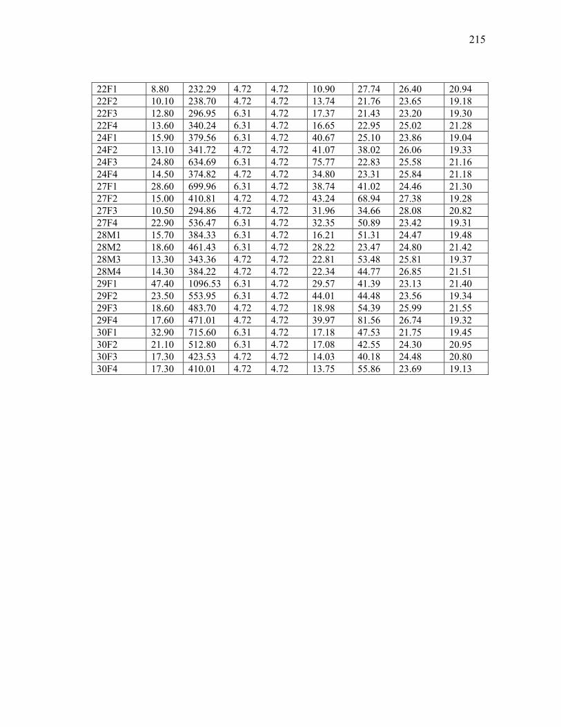
215
22F1 8.80 232.29 4.72 4.72 10.90 27.74 26.40 20.94 22F2 10.10 238.70 4.72 4.72 13.74 21.76 23.65 19.18 22F3 12.80 296.95 6.31 4.72 17.37 21.43 23.20 19.30 22F4 13.60 340.24 6.31 4.72 16.65 22.95 25.02 21.28 24F1 15.90 379.56 6.31 4.72 40.67 25.10 23.86 19.04 24F2 13.10 341.72 4.72 4.72 41.07 38.02 26.06 19.33 24F3 24.80 634.69 6.31 4.72 75.77 22.83 25.58 21.16 24F4 14.50 374.82 4.72 4.72 34.80 23.31 25.84 21.18 27F1 28.60 699.96 6.31 4.72 38.74 41.02 24.46 21.30 27F2 15.00 410.81 4.72 4.72 43.24 68.94 27.38 19.28 27F3 10.50 294.86 4.72 4.72 31.96 34.66 28.08 20.82 27F4 22.90 536.47 6.31 4.72 32.35 50.89 23.42 19.31 28M1 15.70 384.33 6.31 4.72 16.21 51.31 24.47 19.48 28M2 18.60 461.43 6.31 4.72 28.22 23.47 24.80 21.42 28M3 13.30 343.36 4.72 4.72 22.81 53.48 25.81 19.37 28M4 14.30 384.22 4.72 4.72 22.34 44.77 26.85 21.51 29F1 47.40 1096.53 6.31 4.72 29.57 41.39 23.13 21.40 29F2 23.50 553.95 6.31 4.72 44.01 44.48 23.56 19.34 29F3 18.60 483.70 4.72 4.72 18.98 54.39 25.99 21.55 29F4 17.60 471.01 4.72 4.72 39.97 81.56 26.74 19.32 30F1 32.90 715.60 6.31 4.72 17.18 47.53 21.75 19.45 30F2 21.10 512.80 6.31 4.72 17.08 42.55 24.30 20.95 30F3 17.30 423.53 4.72 4.72 14.03 40.18 24.48 20.80 30F4 17.30 410.01 4.72 4.72 13.75 55.86 23.69 19.13

216
APPENDIX M
VALIDATION RESULTS
Observed Estimated Estimation Error Maneuver t2 (s) d2 (m) t2 (s) d2 (m) t2 d2
3M1 18.40 427.99 18.44 428.646 0.19% 0.15% 3M2 18.10 416.38 18.13 417.047 0.19% 0.16% 3M3 27.40 654.55 27.52 657.02 0.42% 0.38% 3M4 17.30 444.40 17.34 445.142 0.20% 0.17% 6M1 25.30 625.15 25.39 627.069 0.35% 0.31% 6M2 16.40 404.52 16.42 404.878 0.10% 0.09% 6M3 22.00 555.17 22.03 555.74 0.16% 0.10% 6M4 9.80 248.16 9.79 247.899 -0.12% -0.11% 7F1 71.30 1625.52 71.01 1618.66 -0.41% -0.42% 7F2 40.40 993.67 40.39 993.465 -0.02% -0.02% 7F3 20.80 529.46 20.85 530.513 0.24% 0.20% 7F4 49.60 1098.40 49.55 1097.58 -0.09% -0.08% 10F1 18.40 494.28 18.39 494.099 -0.04% -0.04% 10F2 30.80 734.63 30.83 735.154 0.10% 0.07% 10F3 22.00 542.34 22.07 543.765 0.31% 0.26% 10F4 41.00 883.78 40.95 882.948 -0.12% -0.09% 11M1 9.70 247.82 9.70 247.874 0.02% 0.02% 11M2 13.70 370.14 13.71 370.408 0.08% 0.07% 11M3 10.40 298.75 10.38 298.33 -0.16% -0.14% 11M4 11.90 284.13 11.90 284.071 -0.03% -0.02% 13F1 17.80 439.40 17.82 439.848 0.12% 0.10% 13F2 23.10 557.22 23.12 557.522 0.09% 0.05% 13F3 21.20 503.18 21.24 504.074 0.20% 0.18% 13F4 16.50 419.63 16.56 421.025 0.39% 0.33% 14M1 8.80 221.63 8.78 221.231 -0.21% -0.18% 14M2 21.40 540.96 21.49 542.812 0.40% 0.34% 14M3 17.00 438.91 17.05 439.913 0.27% 0.23% 14M4 21.60 500.94 21.67 502.373 0.30% 0.29% 17F1 23.50 575.86 23.54 576.635 0.16% 0.13% 17F2 20.30 490.50 20.47 494.399 0.83% 0.80% 17F3 18.30 471.42 18.33 471.981 0.15% 0.12% 17F4 15.40 419.41 15.42 419.777 0.10% 0.09% 18M1 9.60 229.87 9.59 229.655 -0.13% -0.09% 18M2 10.30 245.97 10.26 245.22 -0.35% -0.31% 18M3 16.20 399.85 16.12 398.144 -0.48% -0.43% 18M4 19.70 478.55 19.58 475.976 -0.59% -0.54% 21F1 21.80 542.16 21.85 543.129 0.23% 0.18% 21F2 13.90 393.77 13.89 393.396 -0.10% -0.10% 21F3 11.70 318.55 11.69 318.394 -0.06% -0.05% 21F4 11.90 290.34 11.87 289.757 -0.21% -0.20%

217
22F1 8.80 232.29 8.81 232.518 0.09% 0.10% 22F2 10.10 238.70 10.05 237.697 -0.48% -0.42% 22F3 12.80 296.95 12.77 296.301 -0.23% -0.22% 22F4 13.60 340.24 13.54 338.777 -0.43% -0.43% 24F1 15.90 379.56 15.92 379.914 0.14% 0.09% 24F2 13.10 341.72 13.14 342.446 0.30% 0.21% 24F3 24.80 634.69 24.77 633.78 -0.11% -0.14% 24F4 14.50 374.82 14.51 374.924 0.08% 0.03% 27F1 28.60 699.96 28.66 701.02 0.19% 0.15% 27F2 15.00 410.81 15.02 411.216 0.14% 0.10% 27F3 10.50 294.86 10.48 294.336 -0.17% -0.18% 27F4 22.90 536.47 22.96 537.586 0.25% 0.21% 28M1 15.70 384.33 15.75 385.296 0.30% 0.25% 28M2 18.60 461.43 18.57 460.509 -0.18% -0.20% 28M3 13.30 343.36 13.31 343.512 0.05% 0.04% 28M4 14.30 384.22 14.34 384.985 0.25% 0.20% 29F1 47.40 1096.53 47.50 1098.51 0.21% 0.18% 29F2 23.50 553.95 23.58 555.543 0.35% 0.29% 29F3 18.60 483.70 18.66 484.953 0.32% 0.26% 29F4 17.60 471.01 17.65 472.054 0.30% 0.22% 30F1 32.90 715.60 32.97 717.072 0.22% 0.21% 30F2 21.10 512.80 21.13 513.374 0.14% 0.11% 30F3 17.30 423.53 17.34 424.393 0.23% 0.20% 30F4 17.30 410.01 17.33 410.671 0.18% 0.16%

218
VITA
Jacqueline Marie Jenkins
The University of British Columbia Department of Civil Engineering
2324 Main Mall Vancouver, B.C. Canada V6T 1Z4
Education Ph.D., Civil Engineering, Texas A&M University, August 2004 M.E., Civil Engineering, Texas A&M University, May 2000 Ba.Sc., Civil Engineering, University of Waterloo, April 1996 Academic Awards and Honors Southwest Region University Transportation Center Dr. William J. Harris Award, 2003 Eno Transportation Foundation Fellowship, 2003 Transportation Association of Canada Stantec Scholarship, 2001 National Dean’s List, 2001 Institute of Transportation Engineers (ITE) District 9 Student Paper Award, 2001 AAA Foundation for Traffic Safety Fellowship, January 1999 to December 2002 Professional Experience Graduate Research Assistant, Texas Transportation Institute, Jan. 1999 to Dec. 2003 Collision Investigator, Ryerson Vehicle Safety Research Center, Sep. 1997 to Dec. 1998 Junior Engineer, Marshall Macklin Monaghan, Apr. 1996 to Sep. 1997 Co-op Student, Marshall Macklin Monaghan, Sep. to Dec. 1995 Co-op Student, Toronto Transit Commission, Jan. to Apr. 1995, May to Aug. 1994 Co-op Student, ITX Technologies, Sep. to Dec. 1993 Summer Student, City of Ottawa, May to Aug. 1993, May to Aug. 1992 Professional Registration Professional Engineers of Ontario, License #90481979
Honor Societies Chi Epsilon, National Civil Engineering Honor Society, 2001 Phi Kappa Phi, Honor Society for Academic Excellence, 2001 Professional Memberships American Society of Civil Engineers (ASCE) Institute of Transportation Engineers (ITE)
• •
President, Texas A&M University Student Chapter of ITE, 2001 Corresponding Secretary, Texas A&M University Student Chapter of ITE, 1999
Society of Automotive Engineers (SAE)


![JICA - 国際協力機構 · 2012-09-18 · Transit cargo 3) 4) [insurance] Trucks:148,000 Kip, Passenger cars: 48,000 kip [transit fee] Trucks: 40,000Kip, Passenger cars: 20,000](https://img.dokumen.tips/doc/110x75/5f2645684473ea70a0158682/jica-e-2012-09-18-transit-cargo-3-4-insurance-trucks148000.jpg)