Modeling of a magneto-rheological (MR) fluid damper · PDF file1486 K. K. Ahn et al. / Journal of Mechanical Science and Technol ogy 23 (2009) 1485~1499 safe and does not require either

Journal of Mechanical Science and Technology 23 (2009) 1485~1499 www.springerlink.com/content/1738-494x

DOI 10.1007/s12206-009-0359-7

Journal of Mechanical Science and Technology

Modeling of a magneto-rheological (MR) fluid damper

using a self tuning fuzzy mechanism† Kyoung Kwan Ahn*, Dinh Quang Truong and Muhammad Aminul Islam

School of Mechanical and Automotive Engineering, University of Ulsan, San 29, Muger 2dong, Nam-gu, Ulsan, 680-764, Korea

(Manuscript Received November 17, 2008; Revised December 26, 2008; Accepted February 6, 2009)

--------------------------------------------------------------------------------------------------------------------------------------------------------------------------------------------------------------------------------------------------------

Abstract A magneto-rheological (MR) fluid damper is a semi-active control device that has recently begun to receive more at-

tention in the vibration control community. However, the inherent nonlinear nature of the MR fluid damper makes it challenging to use this device to achieve high damping control system performance. The development of an accurate modeling method for a MR fluid damper is necessary because of its unique characteristics. Our goal was to develop an alternative method for modeling an MR fluid damper by using a self tuning fuzzy (STF) method based on neural tech-nique. The behavior of the researched damper is directly estimated through a fuzzy mapping system. To improve the accuracy of the STF model, a back propagation and a gradient descent method are used to train online the fuzzy pa-rameters to minimize the model error function. A series of simulations were done to validate the effectiveness of the suggested modeling method when compared with the data measured from experiments on a test rig with a researched MR fluid damper. Finally, modeling results show that the proposed STF interference system trained online by using neural technique could describe well the behavior of the MR fluid damper without need of calculation time for generat-ing the model parameters.

Keywords: Magneto-rheological (MR) fluid; Damper; Modeling; Self tuning; Fuzzy --------------------------------------------------------------------------------------------------------------------------------------------------------------------------------------------------------------------------------------------------------

1. Introduction

Many kinds of actuators have been developed and widely used in industry. Among them, the magnetic actuator has been considered and studied since the 1960s. However, it has proven advantages, reliabilities and flexibilities in real applications. Recently, many researches have been conducted on magnetic actuators and magnetic effects.

Vibration suppression is considered key in civil en-gineering to ensure the safety and comfort of the oc-cupants and users of mechanical structures. To reduce the system vibration, an effective vibration control with isolation is necessary. Vibration control tech-

niques have classically been categorized into two areas, passive and active controls. For a long time, efforts were made to make the suspension system work opti-mally by optimizing its parameters, but due to the intrinsic limitations of a passive suspension system, improvements were effective only in a certain fre-quency range. Compared with passive suspensions, active suspensions can improve the performance of the suspension system over a wide range of frequencies. Semi-active suspensions were proposed in the early 1970s [1], and can be nearly as effective as active suspensions. When the control system fails, the semi-active suspension can still work under passive condi-tions. Compared with active and passive suspension systems, the semi-active suspension system combines the advantages of both active and passive suspensions because it provides better performance when com-pared with passive suspensions and is economical,

†This paper was recommended for publication in revised form by Associate Editor Hong Hee Yoo

*Corresponding author. Tel.: +82 52 259 2282, Fax.: +82 52 259 1680E-mail address: [email protected] © KSME & Springer 2009

1486 K. K. Ahn et al. / Journal of Mechanical Science and Technology 23 (2009) 1485~1499

safe and does not require either higher-power actuators or a large power supply as active suspensions do [2].

In early semi-active suspension, many researches on variable orifice dampers were done [3, 4]. With these damper types, the damping force can be regulated by adjusting the orifice area in the oil-filled damper, thus changing the resistance to fluid flow, but adjusting the speed is slow because of mechanical motion limita-tions. Another class of semi-active suspension uses controllable fluids. Two fluids that are viable contend-ers for development of controllable dampers are elec-trorheological (ER) fluids and magnetorheological (MR) fluids. Although the discovery of both ER and MR fluids dates back to the late 1940’s, researchers have primarily concentrated on ER fluids for civil engineering applications [5-8]. Recently developed MR fluids appear to be an attractive alternative to ER fluids for use in controllable fluid dampers [9-12]. MR fluids are smart materials, which typically consist of micron-sized, magnetically polarizable particles dis-persed in a carrier medium such as mineral or silicone oil. The particles form chain-like fibrous structures in the presence of a high electric field or a magnetic field. When the electric field strength or the magnetic field strength reaches a certain value, the suspension solidi-fies and will have high yield stress; conversely, the suspension can be liquefied once more by removal of the electric field or the magnetic field. These materials demonstrate dramatic changes in their rheological behavior in response to a magnetic field [9]. The proc-ess of change is very quick, less than a few millisec-onds, and can easily be controlled by small amounts of energy on the order of several watts. Consequently, MR fluid dampers, which utilize the advantages of MR fluids, are semi-active control devices that are capable of generating a force with magnitude suffi-cient for rapid response in large-scale applications, while requiring only a battery for power [12]. Addi-tionally, these devices offer highly reliable operations and their performance is relatively insensitive to tem-perature fluctuations or impurities in the fluid [9]. As a result, there has been active research and development of MR fluid dampers and their applications [13-18].

However, major drawbacks that hinder MR fluid damper applications are their nonlinear force/dis-placement and hysteretic force/velocity characteristics. One of the challenges involved in creating a high per-formance MR fluid damper in control applications is the development of accurate models that can take full advantage of the unique features of the MR device.

Both parametric and non-parametric models have been built by researchers to describe the behavior of MR fluid dampers. The parametric models based on me-chanical idealizations have been proposed as the Bingham, Bouc-Wen, phenomenological model, and others [19-26]. The Bingham model [19] represents the dry-friction as a signum function on the damper velocity and may be considered as a simple model for describing the hysteresis characteristic. The Bouc-Wen model uses a differential equation to depict the non-linear hysteresis with moderate complexity and is widely applied in building controls. Once the charac-teristic parameters of the Bouc-Wen model are deter-mined, the model can obtain the linearity and the smoothness of the transition from the pre-yield to the post-yield region. One of the major problems in the Bouc-Wen model is the accurate determination of its characteristic parameters, which is obtained by using optimization or trial error techniques. Consequently, these techniques demand high computational cost to generate the model parameters. Moreover, the fact that each set of constant parameters is valid only for single vibration conditions makes the Bouc-Wen model in-appropriate for varying excitation environments. Therefore, many researches on how to develop an MR fluid damper model for higher accuracy and higher adaptability in estimating the behavior of the damper have been done. Spencer et al. [21] successfully de-veloped a phenomenological model to improve the model accuracy with an additional internal dynamical variable. Choi and Lee [22] designed a hysteresis damper model based on a polynomial and curve fit-ting to better predict the damping force when com-pared with conventional models. Dominguez et al. [23, 24] proposed a methodology to find the charac-teristic parameter of Bouc-Wen model and then de-signed a new non-linear model to simulate the behav-ior of the MR fluid dampers. Kwok et al. designed a hysteretic model based on a particle swarm optimiza-tion [25] or using GA technique [26] to modify the Bouc-Wen model and identify the characteristic pa-rameters of the models. The effectiveness of these models with their identification process was proved through the experimental test data. However, the pa-rametric modeling methods require assumptions as regards the structure of the mechanical model that simulates behavior. The approach could be divergent if the initial assumptions for the model structure are flawed, or if the proper constraints are not applied to the parameters. Unrealistic parameters such as nega-

K. K. Ahn et al. / Journal of Mechanical Science and Technology 23 (2009) 1485~1499 1487

tive mass or stiffness may be obtained. Meanwhile, non-parametric methods could avoid these drawbacks of the parametric approaches for modeling, which are adaptive and applicable to linear, nonlinear, and hys-teretic systems. For modeling MR fluid dampers, Chang and Roschke [27] proposed a non-parametric model using multilayer perceptron neural network with optimization method for a satisfactory represen-tation of damper behavior. Schurter and Roschke [28] investigated the modeling of MR fluid dampers with an adaptive neuro-fuzzy inference system. The fuzzy structure was simple for modeling; nevertheless, the training model process relied on input and output information on MR fluid dampers and took much computation time. Wang and Liao [29, 30] explored the modeling of MR fluid dampers by using a trained direct identification based on recurrent neural net-work. Although, the designed models could predict the dynamic responses of the dampers with high pre-cision, the model architectures and the training meth-ods were complex.

For these reasons, a novel direct modeling method to simply model simply MR fluid dampers is proposed in this paper. This method uses a self self-tuning fuzzy (STF) system based on neural technique and was de-signed to overcome the disadvantages of conventional models. Here, an alternative MR fluid damper model built in the form of the simple fuzzy mapping laws, which use uses triangle membership functions (MFs) and centrecenter-average defuzzification, is considered to estimate directly the MR damping force output with respect to the MR characteristics. In order toTo im-prove the accuracy of the proposed STF model, the back propagation learning rules based on gradient descent method is are used to adjust online the fuzzy parameters to minimize the model error function. In-put information for the fuzzy training process is the current supplied for the MR fluid damper and its dy-namic responses. Effectiveness of the proposed MR fluid damper modeling method is clearly verified through comparisons of the experimental data ob-tained from a damper test rig, and modeling results. The results show that the proposed fuzzy interference system trained online by using neural technique has satisfactorily representative ability for the behavior of MR fluid damper with small computational require-ment.

The remainder of this paper is organized as follows. Section 2 describes the test rig using an MR fluid damper. In section 3, some commonly used models

are analyzed and then the procedure of designing the proposed modeling method is presented. Section 4 shows the modeling results of the MR fluid damper using the proposed STF model. Concluding remarks are presented in section 5.

2. Experimental apparatus

To take full advantage of the unique features of the MR fluid damper in control applications, a model must be developed that can accurately reproduce the behavior of MR fluid damper. To verify the precision of the proposed modeling method for an MR fluid damper, a test rig using a specific damper was set up to obtain experimental data used in the modeling process and to compare the real damping response and the MR model output. An MR fluid damper of the RD-1005-3 series manufactured by LORD Corpo-ration was used in this study. The details of the test system are described below.

2.1 MR fluid damper

The MR fluid damper is a damper containing a special fluid, the MR fluid, which is allowed to change its viscosity with respect to an applied exter-nal magnetic field. Here, the MR fluid is a non-magnetic fluid, such as mineral or silicon oil, carrying tiny magnetic particles, such as carbonyl iron. The fluid is housed within a cylinder and flows through a small orifice. A magnetic coil is built in the piston or on the housing. When a current is supplied to the coil, the particles are aligned and the fluid changes from the liquid state to the semi-solid state within millisec-onds. Consequently, a controllable damping force is produced. The force procedure by a linear MR fluid damper depends on magnetic field induced by the current in the damper coil and the piston velocity as in Fig. 1. The damper operates in the flow mode, which means that the produced force is controlled by the flow resistance of the MR fluid portion contained in the gap inside the piston.

The MR fluid damper RD-1005-3 used in this re-search is a compact magneto-rheological fluid dam-per unsurpassed in its combination of controllability, responsiveness and energy density. As a magnetic field is applied to the MR fluid inside the mono-tube housing, the damping characteristics of the fluid in-crease with practically infinite precision. This damper can be adapted to a wide variety of applications be-cause of its simple design, small size, quiet operation,


Table 1. Technical data for the MR fluid damper RD1005-3.

LORD MR fluid damper – RD-1005-3 Series

Parameter Value

Compressed length (mm) 155

Extended length (mm) 208

Weight (g) 800

Magneto-Rheological fluid Viscosity (Pa-s) at 40°C Density (g/cm3) Solids content by weight, % Operating temperature (°C)

MRF-132DG 0.092 ± 0.015 2.98-3.18 80.98 -40 to +130

Electrical characteristics: Maximum input current (A) Input voltage (VDC)

2 12

Mechanical characteristics: Maximum extension force (N) Maximum operating temperature (deg)

4448 71

Response time (ms) (amplifier & power supply depend-ent)

<25 (time to reach 90% of max level during a 0 to 1 amp step input)

Fig. 1. Diagram of an MR fluid damper.

Fig. 2. MR fluid damper RD-1005-3.

Fig. 3. Diagram of the experimental setup.

and compact shock absorption with low voltage and current demands that allow for real-time damping control. The photographs and specifications of the damper are displayed in Fig. 2 and Table 1.

Based on the dimensions and characteristics of the damper RD-1005-3, a rig to perform the damping test and to model the damper was designed and set up as follows.

2.2 Test rig

A schematic diagram of the test rig for the RD-1005-3 damper is depicted in Fig. 3. In the experi-mental system, a hydraulic actuator and a driving controller (VibMaster) manufactured by Park elec-tronics were employed to drive the damper. The data acquisition system consisted of up to eight control axes (synchro or individual), up to four analog input channel users, and four analog output channel users. In the actuator, the servo valve with a nominal opera-tional frequency range of 0-50 Hz, made by Moog Inc., was used as the final control target to adjust the motion. The actuator has a 3.5 cm diameter cylinder and a ±20 mm stroke fitted with low friction Teflon seals to reduce non-linear effects. A linear variable differential transformer (LVDT) was set up to meas-ure the displacement of the piston-rod of the MR fluid damper. In addition, a compatible load cell with 500 kgf capacity by Bongshin was attached in series with the damper rod to measure the damping force. A PC installed with the VibMaster control program was used to generate system vibrations, while the PC with a current amplified circuit sent the current signal to adjust the damper characteristic. Consequently, the feedback signals measured by the LVDT and the load cell were sent back to the PC through an Advantech A/D PCI card 1711 to perform full data acquisition with input and output signals.

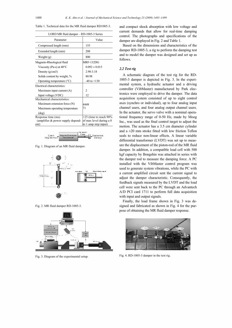
Finally, the load frame shown in Fig. 3 was de-signed and fabricated as shown in Fig. 4 for the pur-pose of obtaining the MR fluid damper response.

Fig. 4. RD-1005-3 damper in the test rig.


3. Modeling of the MR fluid damper with the

STF mechanism

First, some common models used to estimate the behavior of an MR fluid damper are revised. Based on the analysis of those models, the proposed STF model and its designing process are described in de-tail. The experimental data obtained from the testing system is used for model analyses and designs.

3.1 Experimental systems

To obtain the data used to characterize the RD-1005-3 MR fluid damper behavior, a series of ex-periments was conducted under various sinusoidal displacement excitations while simultaneously alter-ing the magnetic coil in a varying current range. The output of each test was the force generated by the damper. The system was excited up to ±5mm by the hydraulic actuator within the frequency range of 1 to 2.5Hz. Likewise, the range of current supplied to the coil inside the damper varied from 0 to 1.5A. A sam-pling time of 0.002 seconds was used to produce Table 2. Parameters setting for the experiments on the MR fluid damper test rig.

Displacement – Sine wave Test No. Amplitude

(mm) Frequency (Hz) MR fluid damper

current (A)

01 to 06 ± 5 1.0 (0,0.5, 0.75, 1.0, 1.25, 1.5)

07 to 12 ± 5 1.5 (0,0.5, 0.75, 1.0, 1.25, 1.5)

13 to 18 ± 5 2.0 (0,0.5, 0.75, 1.0, 1.25, 1.5)

19 to 24 ± 5 2.5 (0,0.5, 0.75, 1.0, 1.25, 1.5)

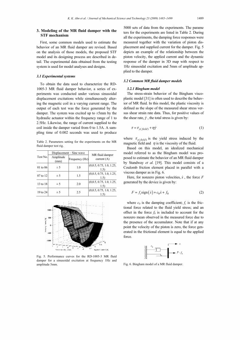
Fig. 5. Performance curves for the RD-1005-3 MR fluid damper for a sinusoidal excitation at frequency 1Hz and amplitude 5mm.

5000 sets of data from the experiments. The parame ters for the experiments are listed in Table 2. During all the experiments, the damping force responses were measured together with the variation of piston dis-placement and supplied current for the damper. Fig. 5 depicts an example of the relationship between the piston velocity, the applied current and the dynamic response of the damper in 3D map with respect to 1Hz sinusoidal excitation and 5mm of amplitude ap-plied to the damper. 3.2 Common MR fluid damper models

3.2.1 Bingham model The stress-strain behavior of the Bingham visco-

plastic model [31] is often used to describe the behav-ior of MR fluid. In this model, the plastic viscosity is defined as the slope of the measured shear stress ver-sus shear strain rate data. Thus, for positive values of the shear rate, γ& , the total stress is given by:

( )y fieldτ τ ηγ= + & (1)

where ( )y fieldτ is the yield stress induced by the magnetic field and η is the viscosity of the fluid.

Based on this model, an idealized mechanical model referred to as the Bingham model was pro-posed to estimate the behavior of an MR fluid damper by Standway et al. [19]. This model consists of a Coulomb friction element placed in parallel with a viscous damper as in Fig. 6.

Here, for nonzero piston velocities, x& , the force F generated by the device is given by:

( ) 0 0signcF f x c x f= + +& & (2)

where c0 is the damping coefficient; fc is the fric-

tional force related to the fluid yield stress; and an offset in the force f0 is included to account for the nonzero mean observed in the measured force due to the presence of the accumulator. Note that if at any point the velocity of the piston is zero, the force gen-erated in the frictional element is equal to the applied force.

Fig. 6. Bingham model of a MR fluid damper.


0.0 0.2 0.4 0.6 0.8 1.0-6

-4

-2

0

2

4

6

Displacement vs. Time

Dis

plac

emen

t [m

m]

Time [s]0.0 0.2 0.4 0.6 0.8 1.0

-1500

-1000

-500

0

500

1000

1500

Force vs. Time

Forc

e [N

]

Time [s]

-6 -4 -2 0 2 4 6

-1500

-1000

-500

0

500

1000

1500

Force vs. Displacement

Forc

e [N

]

Displacement [mm]

Experimental Data Bingham Model Bouc-Wen Model Hysteretic Model

-8 -6 -4 -2 0 2 4 6 8

-1500

-1000

-500

0

500

1000

1500

Force vs. Velocity

Forc

e [N

]

Velocity [cm/s] Fig. 7. Comparison between experimental data and the pre-dicted damping forces for a 2.5Hz sinusoidal excitation with amplitude 5mm while current supplied to the damper is 1.5A.

Fig. 8. Extended Bingham model of an MR fluid damper.

To present the damper behavior, the characteristic

parameters of the Bingham model in Eq. (2) need to be chosen to fit with the experimental data of the damping system. For example, those parameters are chosen as c0 = 50Ns/cm; fc = 950N and f0 = 75N for a 2.5Hz sinusoidal excitation with amplitude 5mm while the current supplied to the damper is 1.5A. Consequently, the predicted damping force by using the Bingham model is compared with the experimen-tal response as plotted in Fig. 7 where the predicted and the measured data are the ‘dash’ and the ‘solid line’, respectively.

From the results, although the force-time and force-displacement behavior are reasonably modeled, the predicted force-velocity relation is not captured, espe-cially for velocities that are near zero. By using this model, the relationship between the force and velocity is one-to-one, but the experimentally obtained data is not one-to-one. Furthermore, at zero velocity, the measured force has a positive value when the accel-eration is negative (for positive displacements), and a negative value when the acceleration is positive (for negative displacements). This behavior must be cap-tured in a mathematical model to adequately charac-terize the device. Hence, Gamota and Filisko [20] developed an extension of the Bingham model, which is given by the viscoelastic-plastic model shown in Fig. 8.

The model consists of the Bingham model in series with a standard model. The governing equations for this model are given as follows:

( ) ( )

( )( )

1 2 1 1 2 1 0

0 1 1 0

2 3 2 0

sign ,c c

F k x x c x x f

c x f x f F f

k x x f

⎫= − + − +⎪⎪= + + >⎬⎪= − + ⎪⎭

& &

& & (3)

( )( )

1 2 1 1 2 0

2 3 2 0, c

F k x x c x fF f

k x x f

⎫= − + + ⎪ ≤⎬= − + ⎪⎭

& (4)

where c0 is the damping coefficient associated with the Bingham model; k1, k2 and c1 are associated with the linear solid material.

This model can present the force-displacement be-havior of the damper better the Bingham model. However, the governing equations (3), (4) are ex-tremely stiff, making them difficult to deal with nu-merically [21]. Therefore, the Bingham model or extended Bingham model is normally employed in case there is a significant need for a simple model.

3.2.2 Bouc-Wen model One model that is numerically tractable and has

been used extensively for modeling hysteretic sys-tems is the Bouc-Wen model. This model contains components from a viscous damper, spring and a hysteretic component. The model can be described by the force equation and the associated hysteretic vari-able as given:

0F cx kx z fα= + + +& (5) 1n nz x z z x z xγ β δ−= − − +& & && (6)

where: F is the damping force; f0 is the offset force; c is the viscous coefficient; k is the stiffness, x& and x are the damper velocity and displacement; α is a scal-ing factor; z is the hysteretic variable; and

, , ,nγ β δ are the model parameters to be identified. Note that when α = 0, the model represents a conven-tional damper.

To determine the Bouc-Wen characteristic parame-ters predicting the MR fluid damper hysteretic re-sponse, Kwok et al. [26] proposed the non-symmetrical Bouc-Wen model with following modi-fications:

( )( ) 0signF c x z kx z fµ α= − + + +& (7)


( ){ }sign nz zx z xγ β δ⎡ ⎤= − + +⎣ ⎦& && (8)

where µ is the scale factor for the adjustment of the velocity.

As the optimization results for the test rig applied the damper RD-1005-3 by using GA in [23], the rela-tionships between the Bouc-Wen parameters and the supplied magnetization current, i, are given as

3 3

3 3

3 3

0

5 5

6 6

6 6

2.65 10 2.05 10 ;

1.99 10 5.57 10 ;

2.11 10 1.68 100.6 12.43; 0.02 1.25;

0.12 1.58

0.5 10 2.5 10 ;

0.45 10 3.18 10 ;

0.39 10 3.6 10

c i

k i

if i in i

i

i

i

αµ

δ

β

γ

= × + ×

= × + ×

= × + ×= − = − += +

= × + ×

= − × + ×

= × + ×

(9)

The Bouc-Wen model built from equations 7 to 9 is

tested for modeling the damping force in this study. As a result, the predicted force is plotted as the ‘dash-dot’ line in Fig. 7 for a 2.5Hz sinusoidal excitation with amplitude 5mm while the current supplied to the damper is 1.5A. From the result, it is clear that to obtain good predicted behavior of an MR fluid dam-per in a specific system, the Bouc-Wen parameters must be tuned by using optimization or trial error techniques, which causes high computational cost to obtain the optimal parameters.

Furthermore, to obtain better modeling perform-ance, some modified Bouc-Wen models have been proposed. The research results in [21] show that the modified Bouc-Wen model improves the modeling accuracy. However, the model complexity is un-avoidably increased with an extended number of model parameters (14 parameters need to be identi-fied in [21]) which may impose difficulties in their identification and take much time for optimization [28].

3.2.3 A hysteretic model For a simple model, Kwok et al. [25] proposed a

hysteretic model to predict the damping force of the MR fluid damper RD-1005-3 as illustrated in Fig. 9. The model can be expressed as the following equa-tions:

Fig. 9. Hysteretic model of an MR fluid damper.

0F cx kx z fα= + + +& (10)

( )( )tanh signz x xβ δ= +& (11)

where: c and k are the viscous and stiffness coeffi-cients; α the scale factor of the hysteresis; z the hys-teretic variable given by the hyperbolic tangent func-tion and f0 is the damper force offset; and ,β δ are the model parameters to be identified.

As the results in [25], the parameters in equations 9 and 10 are given:

20

1929 1232; 1700 5100;

244 918 32; 18 57100; 0.3 0.58

c i k i

i i f ii

αβ δ

= + = − +

= − + + = − += = +

(12)

However, to obtain the parameters as in Eq. (12), a

swarm optimization [26] based on GA algorithm must be used to select the most suitable values with respect to each specific system using the damper RD-1005-3. Hence, when using the set of resulting pa-rameters in [26] to apply to the test system of the MR fluid damper RD-1005-3 in this study, the hysteretic model cannot present well the damper behavior. For example, the modeling result by using the hysteretic model, for a 2.5Hz sinusoidal excitation with ampli-tude 5mm while the current supplied to the damper is 1.5A, is depicted in Fig. 7 as the ‘short dash’ line. The result proves that although the estimated force in this case is better than in case of using Bingham or Bouc-Wen model, the nonlinear characteristic of the damper cannot be described well. Moreover, the swarm optimization also takes training time to gener-ate the parameters of hysteretic model.

3.3 Proposed MR fluid damper model based on STF

From above analyses, the common models can pre-dict the characteristic of an MR fluid damper with high accuracy and applicability. However, the pa-rameters representing those models need to be tuned by using optimization or trial and error techniques,


which causes high computational cost to generate the parameters. In addition, those models only adapt with specific damping systems. For a new system, the optimization process must be done again for a full prediction of the damper behavior. Therefore, a non-parametric method based on intelligent techniques, for example, is an effective solution to estimate di-rectly the MR fluid damper behavior with high preci-sion.

A fuzzy system is an intelligent tool imitating the logical thinking of humans and then is capable of approximating any continuous function. However, there is no systematic method to design and examine the number of rules, input space partitions and mem-bership functions (MFs). Meanwhile, a neural net-work mimics the biological information processing mechanisms. It is typically designed to perform a nonlinear mapping from a set of inputs to a set of outputs. They are non-programmed adaptive informa-tion processing systems that can autonomously de-velop operational capabilities in response to an infor-mation environment. It learns from experience and generalizes from previous examples. This technique modifies its behavior in response to the environment, and is ideal when the required mapping algorithm is unknown and the tolerance to faulty input information is required. Hence an identification system using fuzzy and neural theory can easily be selected as an effective method for directly modeling MR fluid damper purpose.

Here, a newly simple direct modeling method for an MR fluid damper based on the STF mechanism is proposed. This proposed model is based on center-average defuzzification architecture, which is compu-

-8 -6 -4 -2 0 2 4 6 8

-1500

-1000

-500

0

500

1000

1500

Sinusoidal(5mm,1Hz)

Forc

e [N

]

Velocity [cm/s]-8 -6 -4 -2 0 2 4 6 8

-1500

-1000

-500

0

500

1000

1500

Sinusoidal(5mm,1.5Hz)

Forc

e [N

]

Velocity [cm/s]

-8 -6 -4 -2 0 2 4 6 8

-1500

-1000

-500

0

500

1000

1500

Sinusoidal(5mm,2Hz)

Forc

e [N

]

Velocity [cm/s]-8 -6 -4 -2 0 2 4 6 8

-1500

-1000

-500

0

500

1000

1500

Sinusoidal(5mm,2.5Hz)

Forc

e [N

]

Velocity [cm/s]

0.00A 0.50A 0.75A 1.00A 1.25A 1.50A

Fig. 10. Experimental data measured at sinusoidal excitations (frequency range (1, 2.5)Hz and 5mm of amplitude), and supplied current in range (0, 1.5)A.

tationally efficient and well suited for implementation of a nonlinear system. In addition, back propagation is used to decide online the shapes of membership function and fuzzy rules together with the gradient descent method to minimize the modeling error. As a result, the designed fuzzy inference system has higher learning ability that improves the identification qual-ity. The following analyses are used to design the proposed STF model.

The fist factor affecting the dynamic response of the damper is the applied displacement on the piston rod. Fig. 10 displaces the comparison between damp-ing results under various sine excitations with 5mm amplitude and frequency range from 1Hz to 2.5Hz while the supplied current level is in range from 0 to 1.5A. The results show that at fixed current level ap-plied to the damper, the damping force varies due to the piston rod velocity, which is caused by the simul-taneous change of frequency and/or amplitude of the applied excitation.

The second factor affecting the behavior of the damper is the changing of current applied to the dam-per coil. Fig. 11 shows an example of measuring re-sults in plots of force-time, force-displacement, and force-velocity relation with respect to a 2.5Hz sinu-soidal excitation and 5mm of amplitude while the current supplied to the damper is in range between 0 and 1.5A. From this figure, it is readily apparent that:

• The force produced by the damper is not cen-tered at zero. This effect is due to the effect of an accumulator containing high pressure nitrogen gas in the damper. The accumulator helps to prevent cavitations in the fluid during normal

0.0 0.2 0.4 0.6 0.8 1.0

-5

-4

-3

-2

-1

0

1

2

3

4

5


Dis

plac

emen

t [m

m]

Time[s]0.0 0.2 0.4 0.6 0.8 1.0

-1500

-1000

-500

0

500

1000

1500

Force vs. Time

Forc

e [N

]

Time [s]

0.00A 0.50A 0.75A 1.00A 1.25A 1.50A

-6 -4 -2 0 2 4 6

-1500

-1000

-500

0

500

1000

1500


Forc

e [N

]

Displacement [mm]

0.00A 0.50A 0.75A 1.00A 1.25A 1.50A

-8 -6 -4 -2 0 2 4 6 8

-1500

-1000

-500

0

500

1000

1500

Force vs. Velocity

Forc

e [N

]

Velocity [cm/s]

0.00A 0.50A 0.75A 1.00A 1.25A 1.50A

Fig. 11. Experimental data measured at sinusoidal excitation (frequency 2.5Hz, and amplitude 5mm), and within current range (0.5, 1.5)A.


operation and accounts for the volume of fluid displayed by the piston rod as well as thermal expansion of the fluid.

• The greater current level, the greater damping force.

• The force increasing speed is faster at lower cur-rent levels because of the effect of magnetic field saturation.

Based on the above analyses, the damping force of the MR fluid damper depends on the displace-ment/velocity of the damper rod and the current sup-plied for the coil inside the damper. Therefore, the designed STF model contains two parts: one is the neural-fuzzy inference (NFI) that is used to estimate the damping force (u) caused by the displacement of the damper rod, and the other is the scheduling gain fuzzy inference (SGFI), which is used to switch be-tween the damping force levels (k) with respect to the current levels supplied for the MR coil. Consequently, the estimated damping force of the STF model (fMR_est) is computed as a multiple of the NFI esti-mated force and the SGFI gain

_MR estf k u= × (13)

To evaluate the accuracy of the MR model, an error

function (E) is defined by the difference between the damping force (fMR_est) estimated from the MR model and the real damping force obtained from experiment (fMR) when the input conditions (MR current and dis-placement/velocity) for both the model and real MR fluid damper system are the same. Therefore, the error function is expressed by the following equation:

2_0.5( )MR est MRE f f= − (14)

Finally, to improve the identification quality of the

Fig. 12. Structure of identification for a MR fluid damper using proposed STF model.

proposed model, a learning mechanism using neural methodology is used to adjust the fuzzy parameters with the purpose of modeling error minimization. Hence, the overall structure of the proposed STF model for an MR fluid damper is shown in Fig. 12.

3.3.1 Neural-fuzzy inference (NFI) The NFI system takes part in estimating the damp-

ing force caused by the applied displacement to the damper. The NFI set is therefore designed with two inputs (in2, and in3) and one output (u).

The ranges of these inputs are from -1 to 1, and are obtained from the applied displacement, and its de-rivative (velocity) through scale factors chosen from the range of displacement and specification of the MR fluid damper. For each input variable, five triangle membership functions (MFs) are used. Here, “NB”, “NS”, “ZE”, “PS” and “PB” are “Negative Big”, “Negative Small”, “Zero”, “Positive Small” and “Positive Big”, respectively. The centroids of the MFs are set initially at the same intervals and the same shape sizes as in Fig. 13a. Because all of the MFs are triangle shapes, we can express these MFs as follows:

1 2( ) , 1,2.........i ji

iji

x ax j N

bµ

− −= = (15)

where aj is the center of the jth triangle and bj is the width; N is the number of triangles.

The fuzzy reasoning results of outputs are deter-mined by an aggregation operation of fuzzy sets of inputs and the designed fuzzy rules, where the MAX-MIN aggregation method and “centroid” defuzzifica-

(a) Initial membership functions for NFI inputs: in2 (t), in3 (t)

(b) Initial membership functions for NFI output: u (t)

Fig. 13. Initial Membership functions of the NFI inputs and output.


tion method are used. In the proposed neural-fuzzy inference, with a pair of inputs (in2, in3), the output of the proposed neural-fuzzy system can be computed as

1

1

M

j jj

M

jj

w

u

µ

µ

=

=

⎛ ⎞⎜ ⎟⎜ ⎟⎝ ⎠=⎛ ⎞⎜ ⎟⎜ ⎟⎝ ⎠

∑

∑ (16)

where µj and wj are the height and weight of the NFI output, respectively, which are obtained from the rule jth.

The output u of the NFI system has five member-ship functions: “NB”, “NS”, “ZE”, “PS”, and “PB”, with the same meaning as the MFs of the inputs. The ranges of the output are set from -1 to 1. The esti-mated force is then obtained by multiplying the out-put and a scale factor chosen from the specification of the MR fluid damper. The initial output weights are decided from the experimental results with constant supplied current where the damping force values are caused by the corresponding point of input displace-

Table 3. Rules table for neural-fuzzy inference of the STF MR model.

Velocity - in3 Estimated MR force - u NB NS ZE PS PB

NB NB NB NM ZE PB

NS NB NM NM PM PB

ZE NB NM ZE PM PB

PS NB NM PM PM PB

Displacement -

in2

PB NB ZE PM PB PB

0 0.05 0.1 0.15 0.2 0.25 0.3 0.35 0.4 0.45 0.5-5

0

5

Dis

plac

emen

t [m

m] Displacement, Veocity, and Force with respect to Time

0 0.05 0.1 0.15 0.2 0.25 0.3 0.35 0.4 0.45 0.5-10

-5

0

5

10

Vel

ocity

[cm

/s]

0 0.05 0.1 0.15 0.2 0.25 0.3 0.35 0.4 0.45 0.5-2000

-1000

0

1000

2000

Time [sec]

Forc

e [N

]

Fig. 14. Experimental results: displacement, velocity and force vs. time at a sinusoidal excitation (frequency 2.5Hz and ampli-tude 5mm).

ment and velocity. Fig. 14 shows an example of these experiments. Here the force value of compression or extension is not the same even if they have the same velocity because of the nonlinearity of the damper. Therefore, the output weights are not set initially at the same intervals as in Fig. 13(b).

By using the above fuzzy sets of input, output vari-able, experimental data, damper behaviors, and ex-periences, the fuzzy rules for the NFI part of the MR model are described in Table 3. Five membership functions for the each input are used to decide the total twenty five rules by using an IF-THEN structure. Here, one fuzzy rule is composed as follows:

Rule i: IF displacement (in2) is Ai and velocity

(in3) is Bi THEN MR force (u) is Ci (i=1,2, .., 25)

where Ai, Bi, and Ci are the ith fuzzy sets of the input and output variables used in the fuzzy rules. Ai, Bi, and Ci are also the linguistic variable values in2, in3, and u, respectively.

Furthermore, the NFI system is online optimized by using the neural network as mentioned above. The idea of the proposed method is to use a back propaga-tion algorithm to tune the input membership functions shape and the weight of the NFI output during the system operation process to minimize the modeling error. The decisive factors in the inputs MFs aj, bj, and the weights of the outputs wj are automatically updated by using the neuron network. The following set of equations shows the back propagation algo-rithm:

( 1)

( 1)

( 1)

i i ji aji

j i ji bji

j i ji wji

Ea aa

Eb bb

Ew ww

η

η

η

+

+

+

⎫∂= − ⎪∂ ⎪

⎪∂ ⎪= − ⎬∂ ⎪⎪∂ ⎪= −

∂ ⎪⎭

(17)

where ,a bη η and wη are the learning rate which determine the speed of learning; E is the error func-tion defined by (14).

The factor ji

Ew∂∂

in Eq. (17) can be calculated as

_

_

MR est

ji MR est i

fE E uw f u w

∂∂ ∂ ∂=∂ ∂ ∂ ∂

(18)


where:

( ) ( ) ( )__

MR est MRMR est

E e t f t f tf∂ = = −

∂ (19)

_MR estfk

u∂

=∂

(20)

1

iMi

jj i

uw

µ

µ=

∂ =∂ ⎛ ⎞

⎜ ⎟⎜ ⎟⎝ ⎠∑

(21)

The next factors ji

Ea∂∂

in (17) can be computed by:

_

_

MR est i

i MR est i i

fE E ua f u a

µµ

∂∂ ∂ ∂ ∂=∂ ∂ ∂ ∂ ∂

(22)

where _MR est

Ef∂

∂ and _MR estf

u∂

∂ are calculated by

using (19) and (20), respectively.

12

1

( )M

j i jj

Mi

jj

w wu

µ

µµ

=

=

−∂ =∂ ⎛ ⎞

⎜ ⎟⎜ ⎟⎝ ⎠

∑

∑ (23)

2( )ii

i isign x a

a bµ∂ = −∂

(24)

The final factor ji

Eb∂∂

in (17) can be found by:

_

_

MR est i

i MR est i i

fE E ub f u b

µµ

∂∂ ∂ ∂ ∂=∂ ∂ ∂ ∂ ∂

(25)

where _MR est

Ef∂

∂, _MR estf

u∂

∂, and

i

uµ∂∂

is calculated

by using (19), (20), and (23), respectively.

22 ii

i i

x ab bµ −∂ =∂

(26)

With the self learning of neural network technique

and the decreasing of the modeling error, the pro-posed NFI model works more effectively with high

accuracy when compared to the real damping re-sponse.

3.3.2 Scheduling gain fuzzy inference (SGFI) This section provides a description of scheduling

gain fuzzy inference which works as an intelligent switch to tune the damping force levels (k) with re-spect to the current levels supplied for the MR coil. The SGFI system is then designed with a single input (in1) and a single output (k).

The range of the input is from 0 to 1, which is ob-tained from the supplied current through a scale factor chosen from the current range for the MR fluid dam-per coil. Five triangle membership functions, “Z” (Zero), “VS” (Very Small), “S” (Small), “M” (Me-dium), and “B” (Big), are used for this input variable. The centroids of the MFs are set at the same initial intervals and the same shape sizes as in Fig. 15(a). These MFs can then be expressed in the same form as (15).

By using a fuzzy system with the same structure as the NFI system in section 3.3.1, with an input value (in1), the output gain (k) can be computed as

1

1

Q

q qq

Q

qq

w

k

µ

µ

=

=

=∑

∑ (27)

where µq and wq are the height and weight of the SGFI

Table 4. Rules table for scheduling gain inference of the STF MR model.

Supplied Current (in1) Z VS S M B

Damping Force - Gain (k) VS S M B VB

(a) M for SGFI input: in1 (t)

(b) Membership functions for SGFI output: k (t)

Fig. 15. Membership functions of the SGFI inputs and output.


0.1 0.2 0.3 0.4 0.5 0.6 0.7 0.8

-1500

-1000

-500

0

500

1000

1500

Time [s]

For

ce [N

]

Force vs.Time

0A0.5A0.75A1.0A1.25A1.5A

Fig. 16. Damping force response in different current levels at a sinusoidal excitation (frequency 2.5Hz and amplitude 5mm).

output, respectively, which are obtained from the rule qth.

For the output k of the SGFI system, five MFs are used. Here, “VS”, “S”, “M”, “B”, and “VB” are “Very Small”, “Small”, “Medium”, “Big”, and “Very Big”, respectively. The ranges of the output are set from 0 to 1. The output force level is then obtained by multiplying the gain k and a scale factor chosen from the specification of the MR fluid damper. The output weights are decided based on the experimental results and the characteristics of the MR fluid damper. Fig. 16 shows examples of experimental results with dif-ferent current levels supplied to the damper while the generated displacements were the same. Therefore, the output weights are set as in Fig. 15b. By using the above fuzzy sets of input, and output variables, the fuzzy rules for the SGFI part in the MR model are described in Table 4 by using an IF-THEN structure. Finally, the output of the proposed STF MR model (fMR_est) is the multiplication of the NFI output (u) and the SGFI output gain (k) as in Eq. (13).

4. Modeling results and comparisons

In this section, simulations are carried out to evalu-ate the ability of the proposed STF model when com-pared with the measured dynamic responses. The experimental data including the piston displacement and current supplied for the damper coil will be used as the inputs of the suggested MR model (section 3.3). Consequently, the model output, damping force, is directly obtained through the fuzzy mapping system. At that time, the parameters of the STF model are updated after each step of simulation time through the online training process by using the neural technique. Here, the deviation between the predicted force and

0.0 0.2 0.4 0.6 0.8 1.0

-5

-4

-3

-2

-1

0

1

2

3

4

5


Dis

plac

emen

t [m

m]

Time[s]0.0 0.2 0.4 0.6 0.8 1.0

-1500

-1000

-500

0

500

1000

1500

Force vs.Time

Forc

e [N

]

Time [s]

-6 -4 -2 0 2 4 6

-1500

-1000

-500

0

500

1000

1500


Forc

e [N

]

Displacement [mm]-8 -6 -4 -2 0 2 4 6 8

-1500

-1000

-500

0

500

1000

1500

Force vs. Velocity

Forc

e [N

]

Velocity [cm/s]

Experimental Data Proposed STF Model

Fig. 17. Comparison between the estimated force and actual damping force for an applied current range (0, 1.5)A at a sinusoidal excitation (frequency 2.5Hz and amplitude 5mm). measured force is fed back to the learning mechanism (see Fig. 12) inside the STF model as training target. The STF parameters are continuously adjusted in the direction to minimize the modeling error in equation (14) and then, the proposed STF model can accurately capture the force responses of the MR fluid damper in the varying of working conditions.

First, the dynamic responses were measured by do-ing experiments on the test rig with various sinusoidal displacement excitations whose frequency is in the range from 1Hz to 2.5Hz, and 5mm amplitude while the applied current for the damper coil is changed from 0A to 1.5A. Figure 17 shows the modeling re-sults of the proposed STF model in a comparison with the real damping behavior for a 2.5Hz sinusoidal displacement. The results show that with the STF modeling method, the nonlinear characteristic of the MR fluid damper can be directly estimated with high accuracy for both the force/time, force/displacement, and force/velocity relation in despite of the varying of applied current for the damper. The STF model shows a good predicting result especially on low current level. When the value of velocity is high, the pro-posed model describes well the MR fluid damper hysteresis. But in the zero velocity regions, there is some error because of the system compliance and the existing noise in the experimental environment. To obtain high modeling precision as shown in Fig. 17, the STF parameters were online optimized by the learning mechanism with respect to the modeling error cost function. Fig. 18 shows the membership functions of the STF system after training to obtain the better estimated force of the MR fluid damper for a 2.5Hz sinusoidal displacement excitation and 1.5A


of the applied current. As a result, the proposed STF model can predict the damping force with higher accuracy.

Secondly, displacement excitations with a continu-ous variation of frequency were used to fully check the ability of the designed modeling method for vary-ing excitation environments. Since, experimental data were measured from the damping system with the chirp displacement excitations whose frequency was varied from 1Hz to 2.5Hz.

(a) MFs for NFI input in2 (t) after training

(b) MFs for NFI input in3 (t) after training

(c) MFs for NFI output u (t)after training

Fig. 18. MFs of the NFI inputs and output after training.

0.0 0.5 1.0 1.5 2.0 2.5

-5

-4

-3

-2

-1

0

1

2

3

4

5


Dis

plac

emen

t [m

m]

Time[s]0.0 0.5 1.0 1.5 2.0 2.5

-100

-50

0

50

100

Force vs. Time

Forc

e [N

]

Time [s]

-6 -4 -2 0 2 4 6

-100

-50

0

50

100


Forc

e [N

]

Displacement [mm]-8 -6 -4 -2 0 2 4 6 8

-100

-50

0

50

100

Force vs. Velocity

Forc

e [N

]

Velocity [cm/s]


Fig. 19. Comparison between the estimated force and actual damping force for an applied current 0A at a chirp excitation (frequency range (1, 2.5)Hz and amplitude 5mm).

0.0 0.5 1.0 1.5 2.0 2.5

-5

-4

-3

-2

-1

0

1

2

3

4

5


Dis

plac

emen

t [m

m]

Time[s]0.0 0.5 1.0 1.5 2.0 2.5

-1000

-500

0

500

1000

Force vs. Time

Forc

e [N

]

Time [s]

-6 -4 -2 0 2 4 6

-1000

-500

0

500

1000


Forc

e [N

]

Displacement [mm]-8 -6 -4 -2 0 2 4 6 8

-1000

-500

0

500

1000

Force vs. Velocity

Forc

e [N

]

Velocity [cm/s]


Fig. 20. Comparison between the estimated force and actual damping force for an applied current 0.5A at a chirp excita-tion (frequency range (1, 2.5)Hz and amplitude 5mm).

0.0 0.5 1.0 1.5 2.0 2.5

-5

-4

-3

-2

-1

0

1

2

3

4

5


Dis

plac

emen

t [m

m]

Time[s]0.0 0.5 1.0 1.5 2.0 2.5

-1500

-1000

-500

0

500

1000

1500

Force vs. Time

Forc

e [N

]

Time [s]

-6 -4 -2 0 2 4 6

-1500

-1000

-500

0

500

1000

1500


Forc

e [N

]

Displacement [mm]-8 -6 -4 -2 0 2 4 6 8

-1500

-1000

-500

0

500

1000

1500

Force vs. Velocity

Forc

e [N

]

Velocity [cm/s]



0.0 0.5 1.0 1.5 2.0 2.5

-5

-4

-3

-2

-1

0

1

2

3

4

5


Dis

plac

emen

t [m

m]

Time[s]0.0 0.5 1.0 1.5 2.0 2.5

-1500

-1000

-500

0

500

1000

1500

Force vs. Time

Forc

e [N

]

Time [s]

-6 -4 -2 0 2 4 6

-1500

-1000

-500

0

500

1000

1500


Forc

e [N

]

Displacement [mm]-8 -6 -4 -2 0 2 4 6 8

-1500

-1000

-500

0

500

1000

1500

Force vs. Velocity

Forc

e [N

]

Velocity [cm/s]




Figs. 19, 20, 21, and 22 depict the comparisons of the real damping responses and the estimated forces in case of 0A, 0.5A, 1A and 1.5A of the applied cur-rent for the MR fluid damper coil. From these results, it is clear that with the online self tuning ability, the proposed model is strong enough to describe well the nonlinear behavior of the damper under various exci-tation environments, especially in case of low sup-plied current level.

5. Conclusion

A simple, direct modeling method for an MR fluid damper using the STF mechanism has been proposed. Furthermore, a test rig using the MR fluid damper was fabricated to verify the effectiveness of the sug-gested model. Based on the experimental results and modeling results, it is clear that the STF model can predict the force-displacement behavior of the MR damper well with high precision. In addition, the pro-posed STF model with the online self tuning ability based on the neural technique does not require com-putational time to generate the characteristic parame-ters of the model as the common used modeling methods such as Bouc-Wen model. Consequently, the STF model can automatically adjust its parameters to adapt to a damping system containing large nonlin-earities and a working environment under perturba-tion. Based on the proposed model, a controller can be more easily designed to control a suspension sys-tem with high performance.

References

[1] D. Karnopp, M. J. Crosby and R. A. Farwood, Vi-bration control using semi-active force generators, ASME J. Eng. Ind., 96 (2) (1974) 619-626.

[2] K. Yi and B. S. Song, A new adaptive sky-hook control of vehicle semi-active suspensions, Proc. of I Mech E Part D J. of Auto. Eng., 213 (3) (1999) 293-303.

[3] K. Kawashima, S. Unjoh and K. Shimizu, Experi-ments on Dynamics Characteristics of Variable Damper, Proc. of the Japan National Symp. on Structural Response Control, Tokyo, Japan, (1992) 121.

[4] T. Mizuno, T. Kobori, J. Hirai, Y. Matsunaga and N. Niwa, Development of Adjustable Hydraulic Dampers for Seismic Response Control of Large Structure, ASME PVP Conf., (1992) 163-170.

[5] H. P. Gavin, Y. D. Hose and R. D. Hanson, Design and Control of Electrorheological Dampers, Proc. of the First World Conf. on Structural Control, Pa-sadena, CA, (1994) 83-92.

[6] W. C. Park , S. B. Choi , and M. S. Suh, Material characteristics of an ER fluid and its influence on damping forces of an ER damper, Part I: material characteristics, Materials & Design, 20 (6) (1999) 317-323.

[7] W. C. Park , S. B. Choi and M. S. Suh, Material characteristics of an ER fluid and its influence on damping forces of an ER damper, Part II: damping forces, Materials & Design, 20 (6) (1999) 325-330.

[8] S. B. Choi and Y. T. Choi, Sliding Model Control of a Shear-Mode Type ER Engine Mount, KSME Int. J., 13 (1) (1999) 26-33.

[9] J. D. Carlson and K. D. Weiss, A growing attraction to magnetic fluids, J. Machine Design, 66 (15) (1994) 61-64.

[10] J. D. Carlson and M. J. Chrzan, Magnetorheologi-cal Fluid Dampers, U.S. Patent 5277281, 1994.

[11] R. Boelter and H. Janocha, Performance of long-stroke and low-stroke MR fluid damper, Proc. of SPIE, Smart Structures and Materials: Passive Damping and Isolation, San Diego, CA, (1998) 303-313.

[12] S. J. Dyke, B. F. Spencer, Jr, M. K. Sain and J. D. Carlson, Modelling and control of magneto-rheological fluid dampers for seismic response re-duction, Smart Material and Structures, 5 (1996) 565-575.

[13] S. R. Hong, S. B. Choi, Y. T. Choi and N. M. We-reley, Non-dimensional analysis and design of a magnetorheological damper, J. of Sound and Vibra-tion, 288 (4) (2005) 847-863.

[14] S. S. Yoon, S. C. Kang, S. K. Yun, S. J. Kim, Y. H. Kim and M. S. Kim, Safe Arm Design with MR-based Passive Compliant Joints and Viscoelastic Covering for Service Robot Applications, KSME Int. J., 19 (10) (2005) 1835-1845.

[15] K. M. Choi, H. J. Jung, S. W. Cho and I. W. Lee, Application of smart passive damping system using MR damper to highway bridge structure, KSME Int. J., 21 (6) (2007) 870-874.

[16] M. Ahmadian and J. A. Norris, Experimental anal-ysis of magnetorheological dampers when subjected to impact and shock loading, Communications in Nonlinear Science and Numerical Simulation, 13 (9) (2008) 1978-1985.

[17] G. Aydar, C. A. Evrensel, F. Gordaninejad and A.


Fuchs, A Low Force Magneto-rheological (MR) Fluid Damper: Design, Fabrication and Characteri-zation, J. of Intelligent Material Systems and Struc-tures, 18 (12) (2007) 1155-1160.

[18] C. Spelta, F. Previdi, S. M. Savaresi, G. Fraternale and N. Gaudiano, Control of magnetorheological dampers for vibration reduction in a washing ma-chine, Mechatronics, Article in press (2008).

[19] R. Stanway, J. L. Sproston and N. G. Stevens, Non-linear Modelling of an Electro-rheological Vi-bration Damper, J. of Electrostatics, 20 (2) (1987) 167-184.

[20] D. R. Gamota and F. E. Filisko, Dynamic Me-chanical Studies of Electrorheological Materials: Moderate Frequencies, J. of Rheology, 35 (3) (1991) 399-425.

[21] B. F. Spencer, S. J. Dyke, M. K. Sain and J. D. Carlson, Phenomenological Model of a Magneto-Rheological Damper, ASCE J. of Engineering Me-chanics, 123 (3) (1996) 230-238.

[22] S. B. Choi and S. K. Lee, A Hysteresis Model for the Field- dependent Damping Force of a Magneto-rheological Damper, J. of Sound and Vibration, 245 (2) (2001) 375-383.

[23] A. Dominguez, R. Sedaghati and I. Stiharu, Model-ling the hysteresis phenomenon of magnetor-heological dampers, Smart Materials and Structures, 13 (6) (2004) 1351-1361.

[24] A. Dominguez, R. Sedaghati and I. Stiharu, Model-ing and application of MR dampers in semi-adaptive structures, Computers and Structures, 86 (3) (2008) 407-415.

[25] N. M. Kwok, Q. P. Ha, T. H. Nguyen, J. Li and B. Samali, A Novel Hysteretic Model for Magneto-Rheological Fluid Damper and Parameter Identifi-cation Using Particle Swarm Optimization, Sensor and actuators A: Physical, 132 (2) (2006) 441-451.

[26] N. M. Kwok, Q. P. Ha, M. T. Nguyen, J. Li and B. Samali, Bouc-Wen Model Parameter Identification for a MR Fluid Damper Using Computationally Ef-ficient GA, ISA transactions, 46 (2) (2007) 167-179.

[27] C. C. Chang and P. Roschke, Neural network mod-eling of a magnetorheological damper, J. Intell. Ma-ter. Syst. Struct., 9 (9) (1998) 755-764.

[28] K. C. Schurter and P. N. Roschke, Fuzzy Modeling of A Magneto-Rheological Damper Using Anfis, Proc. of IEEE Int. Conf. on Fuzzy Systems, (2000) 122-127.

[29] D. H. Wang and W. H. Liao, Neural Network Modeling and Controllers for Magneto-rheological

Fluid Dampers, Proc. of 10th IEEE Int. Conf. on Fuzzy Systems, (2001) 1323-1326.

[30] D. H. Wang and W. H. Liao, Modeling and Control of Magneto-Rheological Fluid Damper Using Neu-ral Networks, Smart Materials and Structure, 14 (1) (2005) 111-126.

[31] I. H. Shames and F. A. Cozzarelli, Elastic and Ine-lastic Stress Analysis, Prentice Hall, Englewood Cliffs, New Jersey, (1992) 120-122.

[32] L. X. Wang, A Course in Fuzzy Systems and Con-trol, Prentice Hall, 1997.

[33] M. P. Kevin and Y. Stephen, Fuzzy Control, Addi-son Wesley Longman, Menlo Park, CA, 1998.

Kyoung Kwan Ahn received the B.S. degree in the Department of Mechanical Engineering from Seoul National University in 1990, the M. Sc. degree in Mechanical Engineering from Korea Ad-vanced Institute of Science and Technology (KAIST) in 1992 and

the Ph.D. degree from Tokyo Institute of Technology in 1999, respectively. He is currently a Professor in the School of Mechanical and Automotive Engineering, University of Ulsan, Ulsan, Korea. His research interests are design and control of smart actuator using smart mate-rial, fluid power control and active damping control. He is a Member of IEEE, ASME, SICE, RSJ, JSME, KSME, KSPE, KSAE, KFPS, and JFPS.

Dinh Quang Truong received the B.S degree from the de-partment of Mechanical Engi-neering from Hochiminh City University of Technology in 2001. From 2003 to 2006, he worked in the lab of machine design - Mechanical

Department of Hochiminh City University of Technol-ogy. He is currently Ph.D. candidate at University of Ulsan. His research interests focus on designing and con-trol of new hydraulic actuators, applications to hybrid vehicles with saving energy.

Documents

Modeling of a magneto-rheological (MR) fluid damper · PDF file1486 K. K. Ahn et al. / Journal of Mechanical Science and Technol ogy 23 (2009) 1485~1499 safe and does not require either