Embed Size (px)
Citation preview

Iranian Journal of Management Studies (IJMS) 2021, 14(3): 547-564 RESEARCH PAPER
Modeling Asset Pricing Using Behavioral Variables: Fama-
Macbeth Approach
Mohammad Nasiri, Fatemeh Sarraf, Nowrouz Nourollahzadeh, Mohsen Hamidian,
Yadollah Noorifard
Department of Accounting, Faculty of Economics and Accounting, Islamic Azad University, South
Tehran Branch, Tehran, Iran
(Received: May 30, 2020; Revised: October 4, 2020; Accepted:October 27, 2020)
Abstract
Investors generally make decisions based on risk and stock returns, and their decisions are influenced
by two factors, namely macroeconomic variables and microeconomic variables. The behavioral factors
affecting investment decisions are investigated in the area of behavioral finance. In other words,
behavioral finance focuses on specific human behavior attributes and their utilization in asset pricing.
Behavioral asset pricing is the result of applying behavioral finance theories within traditional asset
pricing theories. Although there are many asset-pricing models, due to their weaknesses and
incompleteness as well as the necessity of investigating behavioral factors, this study attempted to
model asset pricing using behavioral models.The population of the study included all listed firms in
Tehran Stock Exchange over the years 2008 to 2018, and the sample was selected through systematic
elimination of the population. Given these conditions, 141 firms were selected as the sample. The
hypotheses were then tested by designing multivariate regression models.The results showed that
using Fama-Macbeth approach, accounting information risk, investors’ trading behavior, and
investors' sentiments had a significant and direct impact on firms’ stock returns.Thus, it is argued that
behavioral variables can play a significant role in Modeling Asset Pricing.
Keywords: Accounting information risk, Investors’ trading behavior,Investors' sentiment stock
returns, Fama-Macbeth approach.
Introduction
The Capital Asset Pricing Model (CAPM) has been a cornerstone of the modern asset pricing
theory (Antypas et al., 2020) that challenges the traditional approach to asset pricing and
argues that judgments in this respect have a short time horizon and are constantly subject to
several risks and costs (De Long et al., 1990). It also argues that prices can somehow be set
through traders' artificial emotions and sentiments, which is mainly true for investors whose
decisions are not based on a thorough analysis of opportunities and are mostly based on
emotionsand unreasonable beliefs (Kumar & Lee, 2006). Financial markets have a
psychological dimension in their true sense (Luo et al., 2014). Behavioral finance is one of the
new topics raised by some financial scholars over the past two decades and has quickly
received the attention of professors, scholars, and students of this field around the world.
According to (Seif Elahi et al., 2015), financial theories have had two different approaches in
recent decades. The first one is the neoclassical approach in financial sciences. According to
this approach, the underlying premise of financial theories is market efficiency and investors’
Corresponding Author, Email: [email protected]
548 Nasiri et al.
rational behavior in the market. This approach began with the Capital Asset Pricing Model
and Efficient Market Theory in the 1960s and the mid-term Capital Asset Pricing Model and
Miller and Modigliani Arbitrage Pricing Theory in the 1970s. Over time and through
conducting different research, researchers noticed many disorders in financial markets, which
could not be justified by efficient market theories. This led to the behavioral revolution in
financial discourses in 1979. On the other hand, theories suggest that risks and errors in asset
pricing are correlated with returns, and the information related to this correlation can be used
to predict future returns. Empirically, pricing models rarely incorporate psychological factors,
but the point is that researchers nowadays can identify influential behavioral factors in
empirical asset pricing models that can seize the manipulation of returns resulting from asset
mispricing (Lin, 2014). As a result, despite the existence of many asset-pricing models, due to
their weaknesses and incompleteness as well as the necessity to investigate behavioral factors,
this study attempted to model asset pricing using behavioral models. Thus, in summary, the
motivators of the present study are the problems of previous models and the weakness in
identifying the role of behavioral factors.In this regard, the Fama-Macbeth model is used
becauseit is a practical way of testing how various factors describe portfolio or asset
returns.This model has survived most of the empirical results to become a standard
methodology in the financial literature for its undeniable merits of simplicity and clarity
(Pasquariello, 1999). Therefore, the question is if we can show (using Fama-Macbeth
approach) that the accounting information risk, investors’ trading behavior, and investors’
sentiment influence firms’ stock returns.
Theoretical Foundations
The purpose of investing in stocks is to receive appropriate returns. Generally, investors’
decision-making is based on risks and stock returns and is influenced by two factors, namely
macroeconomic and microeconomic variables. Macro variables include economic growth,
inflation, etc., which have a general impact on all securities; however, micro economic
variables such as accounting earnings are substantially firmspecific (Chen et al., 2014;Fong &
Toh, 2014). Recognizing these firm-specific factors and relationships can therefore play an
important role in investors and managers’ decision making for deeper analysis and more
efficient use of resources (Bozorg Asl & Razavi, 2008). There are already many asset-pricing
models that explain assets value, but there is still a significant difference between the
theoretical price of securities and their trade value in the market. It seems that other models
need to be sought in order to estimate the price more accurately. One new pricing method is
market-based pricing, which reflects the effect of the behavioral factor of investors' sentiment
on stock pricing. Behavioral Finance Theory states that perceptual errors and sentiments have
a significant impact on financial decision-making (Salehi et al., 2020). Behavioral asset
pricing is the result of applying behavioral finance theories within traditional asset pricing
theories (Xin-ke, 2014). Accounting Information Risk and Stock Returns
Questions about the role of information risk in determining capital cost and whether
information risk is flexible or not remain as unresolved issues in the accounting literature. A
number of recent empirical and theoretical studies have attempted to address this issue. For
example, traditional capital asset pricing model and the Fama and Frenchthree-factor model
do not incorporate any information risk factors (Fama & French, 1993). Contrary to this view,
Easley and O'Hara's (2004) theoretical model assumed that stocks with more confidential

Iranian Journal of Management Studies (IJMS) 2021, 14(3): 547-564 549
information would be more risky because they have more news to be disclosed to investors.
Hughes and Liu also argued that having controlled systematic risk, information asymmetry
would not affect firms’ capital cost. However, they argued that higher information asymmetry
about systemic factors leads to higher capital costs (Hughes & Liu, 2007). Lambert et
al.(2012), too, suggested that in a perfectly competitive market, information asymmetry
cannot influence capital cost, but information accuracy can do so. Besides, in imperfect
markets, information asymmetry and information accuracy play a decisive role in the firm’s
capital cost. Thus, it is argued that in Iran Capital Market, a firm’s accounting information
risk can affect asset returns and pricing.
Trading Behavior, Sentiment, and Stock Returns
Understanding how trading behavior and investors’ sentiment influence stock prices in financial
markets is one of the most important issues in financing. Schiller (2014) emphasized that in the
light of real human behavior, researchers need to consider real thoughts and actions of
individuals. Standard Decision Theory holds the view that individuals act logically and
rationally. Behavioral finance replaces the Behavioral Portfolio Theory with the Mean-Variance
Portfolio Theory, proposes a Behavioral Asset Pricing Model (BAPC) for Capital Asset Pricing
Model (CAPM), and suggests other models that determine expected returns by risks. Behavioral
finance also identifies rational markets for efficient market disputes and tests why many
investors believe it is easy to hit the market. Moreover, while adhering to standard finance,
behavioral finance extends the financial domain beyond the asset pricing portfolio and market
efficiency, (Statman, 2014). According to Ritte (2003), behavioral finance is based on
psychology, and the human decision-making process derives from several cognitive illusions.
Studies of psychology researchers shows that for a variety of reasons, the cognitive process
is not properly performed. As a result, series of cognitive biases that are the source of false
cognition are examined. Due to psychological foundations, human beings are exposed to these
biases, which affect their reactions to the phenomena and the decisions that must be made. Of
course, in different conditions, these biases can occur more or less. However, when it comes to
"false cognition," it is argued that if someone felt out of things, he/she would have different
cognitions and judgments, and now that he/she has been subjected to certain circumstances and
biases, his/her cognitions and judgments have been impressed. Cognitive biases mainly occur in
the absence of information and in uncertainty (Saeedi & Farhanian, 2015). Yet, a large body of
financial literature shows that excess returns cannot be explained easily by fundamental
variables, and numerous studies have concluded that stock returns and a firm's assets value are
influenced by investors’ sentiment. Previous studies have also argued that stock returns are
influenced by the trading behavior of retail or institutional investors. The notable point in these
studies is that retail investors can direct the market (Yang & Zhou, 2015).
Background
Antypaset al. (2020)introduce a methodology that deals with possibly integrated variables in
the specification of the betas of conditional asset pricing models. The results provide evidence
that the residuals of possible cointegrating relationships between integrated variables in the
specification of the conditional betas may reveal significant information concerning the
dynamics of the betas. Chauhan et al. (2019) attempted to find empirical evidence of herding
in two different cross-sections of financial markets using cross-sectional deviations of stock
returns to measure the dispersion of individual stock returns from average market return. They
showed whether the cross-sectional dispersion of stock returns in large-cap stocks were lower

550 Nasiri et al.
compared to that in small-cap stocks, implying stocks with higher market capitalization and
trading volume were less prone to herding. Paraboni et al.(2018) examined the relationship
between sentiment and risk in financial markets. Their results are consistent with Prospect
Theory, indicating that when liquidity is thought to be low, investors try to reduce the
negotiations that positively influence risk. On the other hand, based on the reverse scenario,
when sentiments indicate high liquidity, there is an increase in the volume of negotiations,
and thus, a decrease in risk. In another study, Zaremba and Konieczka (2017) observed that
portfolios which were based on four factors of size (market value), value (book-to-market
value), momentum (annual rate of returns excluding dividends for 12 months prior to
November 31), and liquidity (average daily turnovers in the past month) had positive stock
returns. According to the results of Conrad et al. (2016), there is a negative relationship
between predicted volatility and future returns and a positive relationship between ex ante
skewness and stock returns. Moreover, the predicted returns with negative skewness will
result in higher future returns. Likewise, Adusei (2014)examined the relationship between
inflation and stock market returns. Using the data from Ghana Stock Exchange as an
emerging market, his results showed that in the short run, there was an inverse relationship
between inflation and stock returns, while this relationship would be direct in the long run. In Iran, Kardan et al. (2017)’s results indicated an increase in the explanatory degree of
CAPM by adding sentiment indices. Similarly, Khajavi and Fa’al Qayyum (2016) reported
that earnings announcement had influenced skewness and returns. Accordingly, when
earnings are not announced, the relationship between skewness and returns is negative and
significant, but by earnings announcement, the relationship loses its significance. In addition,
Hejazi et al. (2015) examined the impacts of market, liquidity, and momentum on major stock
price changes. The results showed a significant relationship between the variables under study
and major stock price changes. Among the factors studied, liquidity was the most important
variable to explain the probability of stock price decline, and market was the most influential
variable on the probability of stock price increase.
Hypotheses
Given the explanations in Theoretical Foundations section, the hypotheses are proposed as
follows:
1. Using Fama-Macbeth approach, accounting information risk has a direct and significant
impact on a firm's stock returns.
2. Using Fama-Macbeth approach, investors’ trading behavior has a direct and significant
impact on a firm’s stock returns.
3. Using Fama-Macbeth approach, investors’ sentiment has a direct and significant impact
on a firm’s stock returns.
Methodology
Since conclusions are made by testing the available data, this research will be grouped into
positive theories. On the other hand, managers, investors, and analysts can employ the results
of this study; therefore, in terms of objectives, it is considered as an applied research. In terms
of nature and content, this study is among correlational research, because regression and
correlation techniques will be used to explore the relationships between variables. Thus, in
terms of reasoning, it is considered deductive. Regarding time, it is a longitudinal study. It is
worth mentioning that the proposed models are tested at the level of listed firms in Tehran
Stock Exchange and the results will be summed up.
Iranian Journal of Management Studies (IJMS) 2021, 14(3): 547-564 551
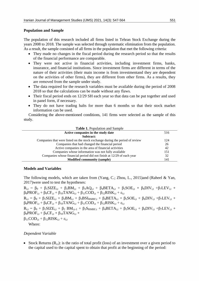
Population and Sample
The population of this research included all firms listed in Tehran Stock Exchange during the
years 2008 to 2018. The sample was selected through systematic elimination from the population.
As a result, the sample consisted of all firms in the population that met the following criteria:
They made no changes in the fiscal period during the research period so that the results
of the financial performance are comparable.
They were not active in financial activities, including investment firms, banks,
insurance, and financial institutions. Since investment firms are different in terms of the
nature of their activities (their main income is from investmentand they are dependent
on the activities of other firms), they are different from other firms. As a results, they
are removed from the sample under study.
The data required for the research variables must be available during the period of 2008
2018 so that the calculations can be made without any flaws.
Their fiscal period ends on 12/29 SH each year so that data can be put together and used
in panel form, if necessary.
They do not have trading halts for more than 6 months so that their stock market
information can be used.
Considering the above-mentioned conditions, 141 firms were selected as the sample of this
study.
Table 1. Population and Sample
516 Active companies in the study date
Subtract:
124 Companies that were listed on the stock exchange during the period of review
26 Companies that had changed the financial period
42 Active companies in the area of financial activities
151 Companies whose information was not fully available
32 Companies whose financial period did not finish at 12/29 of each year
141 Modified community (sample)
Models and Variables
The following models, which are taken from (Yang, C.; Zhou, L., 2015)and (Raheel & Yan,
2017)were used to test the hypotheses:
Ri,t = β0 + β1SIZEi,t + β2BMi,t + β3AQi,t + β4BETAi,t + β5SOEi,t + β6DIVi,t +β7LEVi,t +
β8PROFi,t + β9CFi,t + β10TANGi,t + β11CODi,t + β12RISKi,t + εi,t
Ri,t = β0 + β1SIZEi,t + β2BMi,t + β3BSIRMRF,t + β4BETAi,t + β5SOEi,t + β6DIVi,t +β7LEVi,t +
β8PROFi,t + β9CFi,t + β10TANGi,t + β11CODi,t + β12RISKi,t + εi,t
Ri,t = β0 + β1SIZEi,t + β2 BMi,t-1 + β3SRMRF,t + β4BETAi,t + β5SOEi,t + β6DIVi,t +β7LEVi,t +
β8PROFi,t + β9CFi,t + β10TANGi,t +
β11CODi,t + β12RISKi,t + εi,t
Where:
Dependent Variable
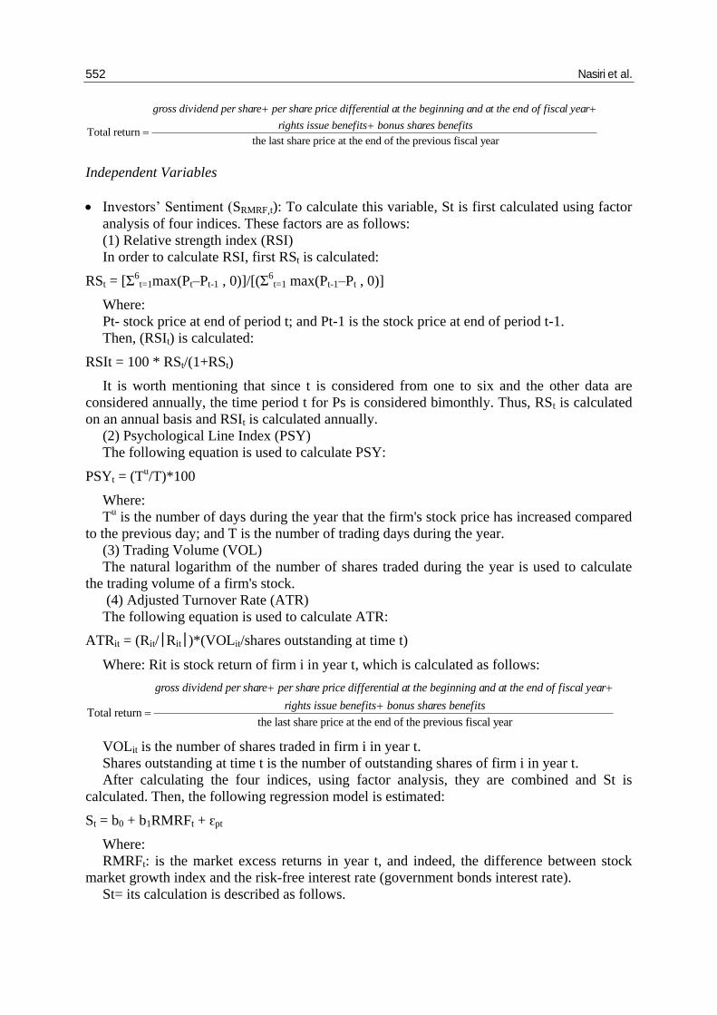
Stock Returns (Ri,t): is the ratio of total profit (loss) of an investment over a given period to
the capital used to the capital spent to obtain that profit at the beginning of the period:
552 Nasiri et al.
Total return the last share price at the end of
gross dividend per share per share price differential at the beginning and at the end of fiscal year
rights issue benefits bonus shares benefits
the previous fiscal year
Independent Variables
Investors’ Sentiment (SRMRF,t): To calculate this variable, St is first calculated using factor
analysis of four indices. These factors are as follows:
(1) Relative strength index (RSI)
In order to calculate RSI, first RSt is calculated:
RSt = [Ʃ6
t=1max(Pt–Pt-1 , 0)]/[(Ʃ6
t=1 max(Pt-1–Pt , 0)]
Where:
Pt- stock price at end of period t; and Pt-1 is the stock price at end of period t-1.
Then, (RSIt) is calculated:
RSIt = 100 * RSt/(1+RSt)
It is worth mentioning that since t is considered from one to six and the other data are
considered annually, the time period t for Ps is considered bimonthly. Thus, RSt is calculated
on an annual basis and RSIt is calculated annually.
(2) Psychological Line Index (PSY)
The following equation is used to calculate PSY:
PSYt = (Tu/T)*100
Where:
Tu is the number of days during the year that the firm's stock price has increased compared
to the previous day; and T is the number of trading days during the year.
(3) Trading Volume (VOL)
The natural logarithm of the number of shares traded during the year is used to calculate
the trading volume of a firm's stock.
(4) Adjusted Turnover Rate (ATR)
The following equation is used to calculate ATR:
ATRit = (Rit/|Rit|)*(VOLit/shares outstanding at time t)
Where: Rit is stock return of firm i in year t, which is calculated as follows:
Total return the last share price at the end of
gross dividend per share per share price differential at the beginning and at the end of fiscal year
rights issue benefits bonus shares benefits
the previous fiscal year
VOLit is the number of shares traded in firm i in year t.
Shares outstanding at time t is the number of outstanding shares of firm i in year t.
After calculating the four indices, using factor analysis, they are combined and St is
calculated. Then, the following regression model is estimated:
St = b0 + b1RMRFt + ԑpt
Where:
RMRFt: is the market excess returns in year t, and indeed, the difference between stock
market growth index and the risk-free interest rate (government bonds interest rate).
St= its calculation is described as follows.
Iranian Journal of Management Studies (IJMS) 2021, 14(3): 547-564 553
The residual of the above model for each firm-year, called SRMRF, will be a criterion for
calculating investors’ sentiment.
Investors’ Trading Behavior (BSIRMRF,t)
To calculate investors’ trading behavior variable, first the following formula needs to be
calculated:
BSIit = (BVit – SVit)/(BVit + SVit)
Where:
BVit is the volume (number) of buying firm i shares during the year t.
SVit is the volume (number) of selling firm i shares during the year t.
After calculating BSIit, the following model is calculated:
BSIit = b0 + b1RMRFt + ԑt
Where:
RMRFt is the market excess returns in year t, or indeed, the difference between the stock
market growth index and the risk-free interest rate (government bonds interest rate).
BSIit is calculated as follows.
The residual of the above model for each firm-year, called BSIRMRF, will be a criterion
for investors’ trading behavior.
Accounting Information Risk (AQi,t):
To calculate accounting information risk, Dicho and Dicho (2002) accruals quality model
modified by Francis et al. (2005) is used:
TCAi,t = b0 + b1CFOi,t-1+ b2CFOi,t + b3CFOi,t+1+ b4∆REVi,t+ b5PPEi,t+ ԑi,t
Where:
TCAi,t= total current accruals of firm i in year t, which is equal to net profit plus
depreciation expense minus operating cash flow divided by total assets.
CFOi,t-1= Operating cash flow of firm i in year t-1, which is equal to operating cash flow
divided by total assets.
CFOi,t= Operating cash flow of firm i in year t, which is equal to operating cash flow
divided by total assets.
CFOi,t+1= The operating cash flow of firm i in year t+1, which is equal to the operating
cash flow divided by total assets.
∆REVi,t= Changes in sales revenue of firm i in year t, which is equal to sales revenue in
year t minus sales income in year t-1 divided by total assets.
PPEi,t= Account of property, plant, and equipment of firm i in year t, which is equal to the
account of property, plant, and equipment divided by total assets.
After estimating the above model at the level of firm totality and calculating the model
coefficient values, the model residual is calculated. Residuals absolute value is used as the
reverse measure of accrual quality and a direct measure for accounting information risk.
Control Variables
SIZEi,t= firm i size in year t, which is equal to the natural logarithm of total assets.
BMi,t-1 = growth opportunities of firm i in year t-1, which is the ratio of the book value of
equity to the market value of equity.
BETAi,t= Systematic risk of firm i in year t which is used to calculate beta coefficient. Beta
coefficient uses the sample firms' stock return (Ri) and market return portfolio (Rm):
β = (Cov(Ri,Rm))/ծ 2Rm
554 Nasiri et al.
SOEi,t= State ownership of firm i in year t. If state ownership exists in the firm, this
variable is set to one, and zero otherwise.
DIVi,t= cash dividend of firm i in year t, which is equal to the ratio of cash dividend per
share to the net profit per share.
LEVi,t= the debt level of firm i in year t, which is equal to debt-to-assets ratio.
PROFi,t= the profitability of firm i in year t, which is equal to the ratio of net profit to
assets.
CFi,t= operating cash flow of firm i in year t, which is the ratio of operating cash to assets.
TANGi,t= tangibility of firm i assets in year t, which is the ratio of tangible assets to total
assets.
CODi,t= cost of debt firm i in year t, which is the ratio of financial costs to total debt.
RISKi,t= risk of firm i in year t, which is the ratio of the standard deviation of the firm's
cash flow over the past three years to assets.
Findings
Descriptive Statistics
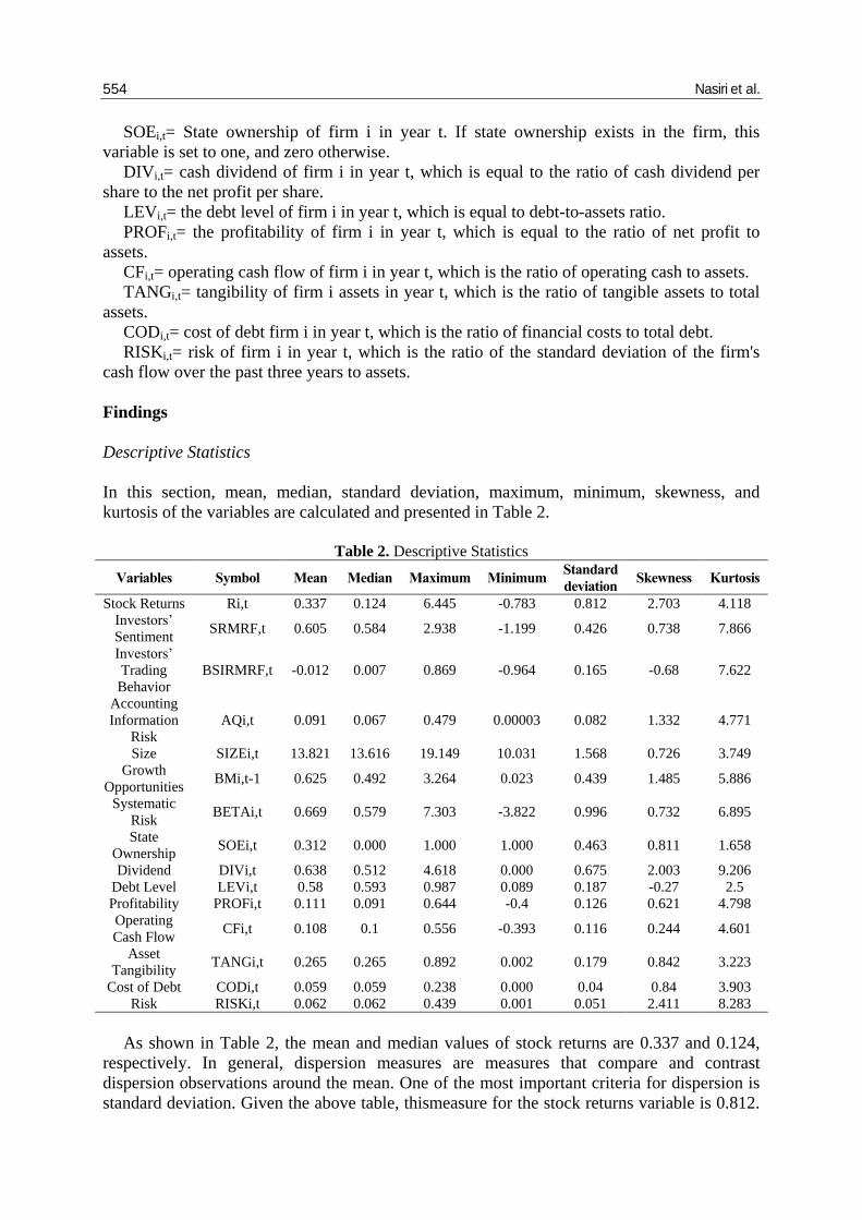
In this section, mean, median, standard deviation, maximum, minimum, skewness, and
kurtosis of the variables are calculated and presented in Table 2.
Table 2. Descriptive Statistics
Kurtosis Skewness Standard
deviation Minimum Maximum Median Mean Symbol Variables
4.118 2.703 0.812 -0.783 6.445 0.124 0.337 Ri,t Stock Returns
7.866 0.738 0.426 -1.199 2.938 0.584 0.605 SRMRF,t Investors’
Sentiment
7.622 -0.68 0.165 -0.964 0.869 0.007 -0.012 BSIRMRF,t
Investors’
Trading
Behavior
4.771 1.332 0.082 0.00003 0.479 0.067 0.091 AQi,t
Accounting
Information
Risk
3.749 0.726 1.568 10.031 19.149 13.616 13.821 SIZEi,t Size
5.886 1.485 0.439 0.023 3.264 0.492 0.625 BMi,t-1 Growth
Opportunities
6.895 0.732 0.996 -3.822 7.303 0.579 0.669 BETAi,t Systematic
Risk
1.658 0.811 0.463 1.000 1.000 0.000 0.312 SOEi,t State
Ownership
9.206 2.003 0.675 0.000 4.618 0.512 0.638 DIVi,t Dividend
2.5 -0.27 0.187 0.089 0.987 0.593 0.58 LEVi,t Debt Level
4.798 0.621 0.126 -0.4 0.644 0.091 0.111 PROFi,t Profitability
4.601 0.244 0.116 -0.393 0.556 0.1 0.108 CFi,t Operating
Cash Flow
3.223 0.842 0.179 0.002 0.892 0.265 0.265 TANGi,t Asset
Tangibility
3.903 0.84 0.04 0.000 0.238 0.059 0.059 CODi,t Cost of Debt
8.283 2.411 0.051 0.001 0.439 0.062 0.062 RISKi,t Risk
As shown in Table 2, the mean and median values of stock returns are 0.337 and 0.124,
respectively. In general, dispersion measures are measures that compare and contrast
dispersion observations around the mean. One of the most important criteria for dispersion is
standard deviation. Given the above table, thismeasure for the stock returns variable is 0.812.

Iranian Journal of Management Studies (IJMS) 2021, 14(3): 547-564 555
It is worth mentioning that the highest value of stock returns is 6.445 and its lowest value is -
0.778. The skewness and kurtosis of the mentioned variable are 2.703 and 4.818, respectively.
Another variable considered in this study is investor’s sentiment, and its maximum and
minimum values are 2.938 (owned by Indamin Shock Absorber Company in 2009) and -1.199
(owned by Alumrad Company in 2015).
Inferential Statistics
1. Estimating Accounting Information Risk Model (Accruals)
In order to estimate accrual quality model coefficients, Chaw and Hausman (Azar & Momeni,
2005) (…) tests were used to identify an appropriate method for estimating the model (Table
3).
Table 3. Chaw and Hausman Test Results
Tests Tests Statistics Significance Level H0 H1
Chaw (fixed effects
vs. panel) 15.111 0.000
Using panel data
method
Using fixed effects
method
Result Rejected Confirmed
Hausman (fixed
effects vs. random
effects
139.252 0.000 Using random
effects method
Using fixed effects
method
Result Rejected Confirmed
According to Table 3, the fixed effects method is preferable to the other two methods;
therefore, the model was estimated using the fixed effects method. The results are presented
in Table 4.
Table 4. Accounting Information Risk (Accruals) Test Results
TCAi,t = b0 + b1CFOi,t-1+ b2CFOi,t + b3CFOi,t+1+ b4∆REVi,t + b5PPEi,t + ԑi,t
Variable Coefficients SD T statistics Significance level VIF
Fixed value 0.133 0.005 24.533 0.000 -
Previous year's
operating cash
flow
0.102 0.015 6.497 0.000 1.28
Current year's
operating cash
flow
-0.873 0.152 -5.727 0.000 1.436
Next year’s
operating cash
flow
0.102 0.014 7.123 0.000 1.365
Changes in sales
revenue 0.098 0.007 13.916 0.000 1.017
Accounts of
property, plant,
and equipment
-0.14 0.016 -8.532 0.000 1.064
F statistics 35.143 R-squared 0.821
F statistics significance level 0.000 Adjusted R-squared 0.798
White diagonal correction (eliminating possible
effects of heteroscedasticity) Dourbin-Watson value 1.828
According to the results of Table 4 and the described approach, the values of accounting
information risk (accruals) are calculated.

556 Nasiri et al.
2. Factor Analysis of Four Variables of RSI, PSY, VOL, and ATR in Order to Calculate
Investors’ Sentiment
As explained earlier, after calculating the four variables of RSI, PSY, VOL, and ATR using
the factor analysis approach, a single variable, named St, was defined, which was used in the
regression model for calculating the investor’s sentiment variable. The reason for employing
factor analysis was that it has the ability to put together the various variables in a balanced
way and according to their values, and then combine them. Thus, the most appropriate
solution for combining multiple variables and forming a new one is factor analysis. Factor
analysis is used to identify the underlying variables of a phenomenon or to summarize a set of
data. The primary data for factor analysis are correlation matrixes between the variables.
Table 5. Factor Analysis of RSI, PSY, VOL, and ATR
Factor loading Headings 0.005 RSI 0.36 PSY
0.008 VOL 0.774 ATR 0.525 KMO index
455.187 Bartlett test statistic 0.000 Bartlett test significance level
Given the KMO index value, which is above 0.5, the identified factors were suitable for
factor analysis. In addition, since the significance level of Bartlett's test is less than 0.05,
factor analysis has been successful. As shown in Table 5, the variable coefficients are used as
a weight in calculating the mean value.
3. Estimating Investors’ Sentiment Model
In order to estimate the coefficients of the investors’ sentiment model, Chaw and Hausman
tests were used to determine an appropriate method for estimating the model (Table 6).
Table 6. Chaw and Hausman Test Results
Tests Test Statistic Significance Level H0 H1 Chaw (fixed effects
vs. panel) 1.394 0.000
Using panel data method
Using fixed effects method
Result Rejected Confirmed Hausman (fixed
effects vs. random effects
22.922 0.000 Using random effects method
Using fixed effects method
Result Rejected Confirmed
As is evident in Table 6, fixed effects method is preferred over the other two methods, and
hence, the model is estimated using fixed effects method. The results are presented in Table 7.
Table 7. Investors’ Sentiment Model Test Results
St = b0 + b1RMRFt + ԑpt Variable Coefficients SD T statistic Significance level VIF
Fixed value 0.06 0.006 9.022 0.000 - Market Excess
Returns 0.22 0.015 13.991 0.000 1.000
F statistic 32.765 R-squared 0.536 F Statistic Significance Level 0.000 Adjusted R-squared 0.51 White diagonal correction (eliminating possible
effects of heteroscedasticity) Dourbin-Watson value 2.084

Iranian Journal of Management Studies (IJMS) 2021, 14(3): 547-564 557
According to the results of Table 6 and the described approach, the values of investors'
sentiment are calculated.
4. Estimating Investors’ Trading Behavior Model
In order to estimate the coefficients of investors' trading behavior model, Chaw and Hausman
tests are used to identify an appropriate method for estimating the model (Table 8).
Table 8. Chaw and Hausman Test Results
Tests Test Statistic Significance Level H0 H1
Chaw (fixed effects
vs. panel)
3.917 0.000 Using panel data
method
Using fixed effects
method
Result Rejected Confirmed
Hausman (fixed
effects vs. random
effects
23.827 0.000 Using random
effects method
Using fixed effects
method
Result Rejected Confirmed
As can be seen in Table 8, fixed effects method is preferred over the other two methods, and
thus, the model is estimated using fixed effects method. The results are presented in Table 9.
Table 9. Investors’ Trading Behavior Model Test Results
BSIit = b0 + b1RMRFt + ԑt
Variable Coefficients SD T statistic Significance level VIF
Fixed value 0.107 0.011 9.259 0.000 -
Market Excess
Returns 0.3 0.101 2.961 0.003 1.000
F statistic 12.718 R-squared 0.617
F Statistic Significance Level 0.000 Adjusted R-squared 0.573
White diagonal correction (eliminating possible
effects of heteroscedasticity) Dourbin-Watson value 2.099
Given the results of Table 9 and the described approach, the values of investors' trading
behavior are calculated.
5. Estimating H1 Model
In order to estimate the coefficients of H1, Chaw and Hausman tests were used to identify an
appropriate method for estimating the model (Table 10).
Table 10. Chaw and Hausman Test Results
Test Test Statistic Significance Level H0 H1
Chaw (fixed effects
vs. panel) 8.543 0.000
Using panel data
method
Using fixed effects
method
Result Rejected Confirmed
Hausman (fixed
effects vs. random
effects
17.962 0.000 Using random
effects method
Using fixed effects
method
Result Rejected Confirmed
As is evident in Table 10, fixed effects method is preferred over the other two methods, and
thus, the model is estimated using fixed effects method. The results are presented in Table 11.

558 Nasiri et al.
Table 11. Results of Estimating H1 Ri,t = β0 + β1SIZEi,t + β2BMi,t + β3AQi,t + β4BETAi,t + β5SOEi,t + β6DIVi,t + β7LEVi,t + β8PROFi,t + β9CFi,t +
β10TANGi,t + β11CODi,t + β12RISKi,t + εi,t
VIF Significance
level T statistic SD Coefficients Variables
- 0.000 4.641 0.237 1.102 Fixed value
1.148 0.000 -5.019 0.01 -0.051 Size
1.315 0.001 -3.239 0.308 -0.999 Growth opportunities
2.209 0.000 5.885 0.064 0.38 Accounting information risk
1.12 0.000 4.386 0.17 0.746 Systematic risk
1.1 0.000 8.146 0.031 0.257 State ownership
1.078 0.000 9.398 0.025 0.235 Dividend
1.714 0.000 5.498 0.203 1.117 Debt level
2.125 0.000 7.895 0.524 4.143 Profitability
1.397 0.000 -6.632 0.035 -0.237 Operating cash flow
1.133 0.000 -6.325 0.037 -0.235 Asset tangibility
1.203 0.002 3.05 3.682 11.232 Cost of debt
1.034 0.000 -7.535 -0.066 -0.504 Risk
0.653 R-squared 25.398 F statistic
0.643 Adjusted R-squared F statistic significance level
2.112 Dourbin-Watson value White diagonal correction (eliminating possible effects of
heteroscedasticity)
Given the results of Table 11, since the t statistic of accounting information risk is greater
than + 1.965 and its significance level is less than 0.05, a significant and direct relationship is
established between accounting information risk and stock returns. Thus, the first hypothesis
– i.e., using Fama-Macbeth approach, accounting information risk has a direct and significant
impact on the firm stock returns – is confirmed.
6. Estimating H2 Model
In order to estimate the coefficients of H2, Chaw and Hausman tests were used to determine
an appropriate method for estimating the model (Table 12).
Table 12. Chaw and Hausman Test Results
Test Test Statistic Significance level H0 H1
Chaw (fixed effects
vs. panel) 7.981 0.000
Using panel data
method
Using fixed effects
method
Result Rejected Confirmed
Hausman (fixed
effects vs. random
effects
23.809 0.000 Using random
effects method
Using fixed effects
method
Result Rejected Confirmed
As can be seen in Table 12, fixed effects method is preferred over the other two methods;
thus, the model is estimated using fixed effects method. The results are presented in Table 13.
According to the results of Table 13, since t statistic of investors’ trading behavior is
greater than + 1.965 and its significance level is less than 0.05, there is a significant and direct
relationship between investors’ trading behavior and stock returns. Therefore, the second
hypothesis of the study – which states using Fama-Macbeth approach, investors' trading
behavior has a direct and significant impact on the firm stock returns – is confirmed.

Iranian Journal of Management Studies (IJMS) 2021, 14(3): 547-564 559
Table 13. Results of Estimating H2 Ri,t = β0 + β1SIZEi,t + β2BMi,t + β3BSIRMRF,t + β4BETAi,t + β5SOEi,t + β6DIVi,t + β7LEVi,t + β8PROFi,t +
β9CFi,t + β10TANGi,t + β11CODi,t + β12RISKi,t + εi,t VIF Significance level T statistic SD Coefficients Variables
- 0.000 8.077 0.16 1.292 Fixed value 1.133 0.02 -2.328 0.02 -0.047 Size 1.245 0.021 -2.298 0.288 -0.663 Growth opportunities 1.041 0.000 9.634 0.797 7.682 Investors’ trading behavior 1.116 0.000 4.154 0.153 0.637 Systematic risk 1.1 0.000 8.148 0.04 0.328 State ownership
1.052 0.000 5.894 0.026 0.156 Dividend 1.61 0.000 6.757 0.243 1.646 Debt level 2.221 0.000 10.022 0.161 1.622 Profitability 1.403 0.000 -3.619 0.038 -0.138 Operating cash flow 1.132 0.000 -5.911 0.036 -0.216 Asset tangibility 1.193 0.014 2.44 3.242 7.914 Cost of debt 1.031 0.000 -13.484 0.042 -0.572 Risk 0.691 R-squared 25.398 F statistic 0.673 Adjusted R-squared F statistic significance level
2.109 Dourbin-Watson value White diagonal correction (eliminating possible effects of
heteroscedasticity)
7. Estimating H3 model
In order to estimate the coefficients of H3, Chaw and Hausman tests were used to determine
an appropriate method for estimating the model (Table 14).
Table 14. Chaw and Hausman Test Results
Test Test Statistic Significance level H0 H1
Chaw (fixed effects vs. panel)
8.445 0.000 Using panel data
method Using fixed effects
method Result Rejected Confirmed
Hausman (fixed effects vs. random
effects 26.717 0.000
Using random effects method
Using fixed effects method
Result Rejected Confirmed
As illustrated in Table 14, fixed effects method is preferable to the other two methods; hence,
the model is estimated using fixed effects method. The results are presented in Table 15.
Table 15. Results of Estimating H3
Ri,t = β0 + β1SIZEi,t + β2 BMi,t-1 + β3SRMRF,t + β4BETAi,t + β5SOEi,t + β6DIVi,t + β7LEVi,t + β8PROFi,t + β9CFi,t + β10TANGi,t + β11CODi,t + β12RISKi,t + εi,t
VIF Significance level T statistic SD Coefficients Variables - 0.000 6.129 0.173 1.065 Fixed value
1.138 0.000 -3.838 0.014 -0.056 Size 1.239 0.002 -3.043 0.287 -0.873 Growth opportunities 1.008 0.000 3.882 0.282 1.097 Investors’ sentiment 1.114 0.000 4.585 0.145 0.668 Systematic risk
1.1 0.000 5.452 0.071 0.39 State ownership 1.053 0.000 7.267 0.019 0.141 Dividend 1.593 0.000 4.754 0.24 1.143 Debt level 2.194 0.032 2.136 1.553 3.318 profitability 1.399 0.000 -5.681 0.02 -0.115 Operating cashflow 1.122 0.000 -3.516 0.03 -0.107 Asset tangibility 1.184 0.003 2.966 3.371 9.999 Cost of debt 1.029 0.002 -3.011 0.171 -0.516 Risk 0.659 R-squared 26.792 F statistic 0.65 Adjusted R-squared 0.000 F statisticsignificancelevel
2.121 Dourbin-Watson value White diagonal correction (eliminating possible effects of
heteroscedasticity)
560 Nasiri et al.
According to the results of Table 15, since t statistic of investors’ sentiment variable is
greater than + 1.965 and its significance level is less than 0.05, a significant and direct
relationship is established between investors’ sentiment and stock returns. Thus, the fifth
hypothesis of the study – which states using Fama-Macbeth approach, investors' sentiment
has a direct and significant impact on the firm stock returns – is confirmed.
Conclusion
In order to test the first hypothesis of the study – which suggests using Fama-Macbeth
approach, accounting information risk has a direct and significant impact on the firm stock
returns – a model consisting of a dependent variable of stock returns and an independent
variable of accounting information risk was used. The results showed that using Fama-
Macbeth approach, accounting information risk has a direct and significant impact on the firm
stock returns. In this regard, it is worth noting that, according to Fama and Laffer, information
has three major benefits, namely reducing risk, improving the firm operating decisions, and
making abnormal earnings in trading securities through gaining access to new confidential
information. It is worth mentioning that in the past, financial reporting was solely taken into
account in terms of regulatory purposes, but since the 1960s, attention was shifted to
providing users with the information they need to make economic decisions (Higson, 2003).
Therefore, the information hypothesis is an alternative or a complement to the supervision
hypothesis. One reason for demanding audited financial statements is to provide useful
information for investors’ decision-making. According to the financial literature on
investment models, the value of a firm is determined by calculating the net present value of
future cash flows. Research evidence also suggests that there is a high correlation between
future cash flows and accounting information reflected in financial statements (Fama &
French, 1993). Given the aforementioned points, it is argued that investors’ sentiment,
investors’ trading behavior, and accounting information risk play a significant role in defining
stock returns and asset pricing. This result is in accordance with the results of Jorgensen and
Li Jing (2012),Choi and Lee (2017), and Hejazi et al.(2015), but it is in contrast with the
results of Khajavii and Fa’al Qayyum (2016).
In order to test the second hypothesis of the study – which states using Fama-Macbeth
approach, investors’ trading behavior has a direct and significant impact on the firm stock
returns – a model consisting of a dependent variable of stock returns and an independent
variable of investors’ trading behavior was used. The results showed that using Fama-
Macbeth approach, investors' trading behavior has a direct and significant effect on the firm
stock returns. In this respect, it is worth noting that Schiller (2014)emphasized that in the light
of real human behavior, researchers need to take into account real human actions and
thoughts. Standard decision theory holds the view that individuals act rationally and logically.
Behavioral finance replaces the Behavioral Portfolio Theory with the Mean-Variance
Portfolio Theory and proposes a Behavioral Asset Pricing Model (BAPC) for Capital Asset
Pricing Model (CAPM), and suggests other models that determine expected returns by risks.
Behavioral finance also identifies rational markets in efficient market disputes, and tests the
reason for which many investors believe it is easy to hit the market. Moreover, while it
adheres to standard finance, behavioral finance extends the financial domain beyond the asset-
pricing portfolio and market efficiency. Behavioral finance is based on psychology, and it
suggests that the human decision-making process derives from several cognitive illusions.
Studies of psychology researchers show that for a variety of reasons, the cognitive process is
not properly performed. As a result, series of cognitive biases that are the source of false
cognition are examined. Due to psychological foundations, human beings are exposed to these
Iranian Journal of Management Studies (IJMS) 2021, 14(3): 547-564 561
biases that affect their reactions to the phenomena and decisions that must be made. Of
course, these biases can manifest more or less in different conditions. However, when it
comes to "false cognition," it is argued that if someone felt out of things, he/she would have
different cognitions and judgments, and now that he/she has been subjected to certain
circumstances and biases, his/her cognitions and judgments have been impressed. Cognitive
biases mainly occur in the absence of information and in uncertainty (Saeedi & Farhanian,
2015). Yet, a large body of financial literature shows that excess returns cannot be explained
easily by fundamental variables, and numerous studies have also concluded that stock returns
and a firm's assets value are influenced by investors’ sentiment. Previous studies have also
argued that stock returns are influenced by the trading behavior of retail or institutional
investors. The notable point in these studies is that retail investors can direct the market (Yang
& Zhou, 2015). This result is in accordance with the results of Kumar and Lee (2006), Li et
al.(2018), Paraboni et al.(2018), and Seif Elahi et al.(2015), butin contrast with the results of
Derakhshandeh and Ali Ahmadi (2017).
To test the third hypothesis of the study – which suggests using Fama-Macbeth approach,
investors' sentiments have a direct and significant impact on the firm stock returns – a model
comprised of a dependent variable of stock returns and an independent variable of investors’
sentiment was employed. The results showed that using Fama-Macbeth approach, investors'
sentiments have a direct and significant impact on the firm stock returns. In this regard, it
should be noted that understanding how investors’ sentiment influences stock prices in
financial markets is one of the most important issues in financing. However, a large body of
the financial literature has shown that excess stock returns cannot be easily explained by
fundamental variables, and numerous studies have also found that a firm’s stock returns are
influenced by investors’ sentiment. In addition, some recent studies have used the investors’
sentiment index to examine the role of investors’ sentiment in explaining the stock returns of
firms listed in the US Stock Exchange. Previous studies have also argued that stock returns
are influenced by retail investors or institutional investors’ sentiment, and many recent studies
have used trading data to classify sellers and buyers transactions and determine a pattern for
investors’ sentiment. The remarkable point in these studies is that retail investors can direct
the market. This result is consistent with the results of Conrad et al.(2016),Li et al. (2018),
Luo (2014), Kardan et al.(2017), and Yang and Zhou (2015), butit is in contrast with the
results of Derakhshandeh and Ali Ahmadi (2017).
Recommendations
Given the results of testing the first hypothesis – which suggests using Fama-Macbeth
approach, accounting information risk has a direct and significant impact on the firm stock
returns – it is suggested to investors in Tehran Stock Exchange and market analysts to
consider that an increase in the risk level of firms’ financial and accounting information can
bring higher returns on investments. Researchers believe that taking risks in investments with
a higher risk level is greater. The principle that higher returns are possible only by taking
higher risks reflects the fact that one cannot take risks and gain returns, and on the other hand,
if the investment takes a higher risk, one should naturally expect higher returns.
According to the second hypothesis of the study, investors in Tehran Stock Exchange and
market analysts are suggested to take into account that investors’ trading behavior - including
informed and uninformed trading- can affect the value of a firm's assets and returns. Thus,
investors in the capital market can assess and predict stock returns of firms in the capital
market by following the investing behavior of other investors and the market totality.

562 Nasiri et al.
Given the results of testing the third hypothesis, it is suggested to investors in the capital
market to consider the fact that if investors' sentiment to trade a particular firm’s stock
increases, the stock returns of that firm will increase, too. This is also useful for capital market
analysts so that they can maximize returns.
It is worth mentioning that in this study, the listed manufacturing firms in Tehran Stock
Exchange were used as the research population. Therefore, it is suggested that in the future
studies, banks and financial institutions listed in Tehran Stock Exchange as well as the listed
firms in Over the Counter (OTC) might be used as the research population. Besides, one of
the independent variables of this study was the firm’s accounting information risk, and Ditcho
and Ditcho accruals quality model adjusted by Francis et al. (2005) was utilized to measure it.
Therefore, researchers and students are suggested to use other criteria such as the model of
Jones accruals model, modified Jones, etc. in future studies and compare the results.
Iranian Journal of Management Studies (IJMS) 2021, 14(3): 547-564 563
References
Adusei, M. (2014). The Inflation-Stock market returns Nexus: Evidence from the Ghana Stock
Exchange. Journal of Economics and International Finance, 6(2), 38-46.
Azar, A., & Momeni, M. (2005). Statistics and its application in management. Tehran: Samat.
Antypas, A., Caporale, G., Kourogenis, N., & Pittis, N. (2020). Estimation of conditional asset pricing
models with integrated variables in the beta specification. Research in International Business
and Finance, 52, 101-148.
Bozorg Asl, M., & Razavi, S. M. (2008). The relationship between stock returns of listed firms in
Tehran Stock Exchange and some macroeconomic variables. Experimental Studies of Financial
Accounting, 27, 97-118.
Chauhan, Y., Ahmad, N., Aggarwal, V., & Chandrad, A. (2019). Herd behavior and asset pricing in
the Indian Stock Market. IIMB Management Review,…32(2),143-152doi:
https://doi.org/10.1016/j.iimb.2019.10.008.
Chen, Z., Lin, W. T., Ma, C., & Tsai, S. (2014). Liquidity provisions by individual investor trading
prior to dividend announcements: Evidence from Taiwan. The North American Journal of
Economics and Finance, 28, 358–374.
Choi, Y., & Lee, S. S. (2017). Realized skewness and future stock returns:The role of
information.Economics, 7(3), 359-378.
Conrad, J., Robert, F. D., & Eric, G. (2016). Ex ante skewness and expected stock returns. Journal of
Finance, 68(1), 85-124.
De Long, J., Shleifer, A., Summers, L., & Waldmann, R. (1990). Noise trader risk in financial
markets. Journal of Political Economy, 98(4), 703-738.
Derakhshandeh, S. H., & Ali Ahmadi, S. (2017). Assessing the role of investors' beliefs on price
orientation and trading volume in the capital market. Financial Knowledge of Securities
Analysis, 10(33), 51-63.
Easley, D., & O'hara, M. (2004). Informationandthe cost of capital. The Journal of Finance, 59, 1553-
1583.
Fama, E. F., & French, K. R. (1993). Common risk factors in the returns on stocks and bonds. Journal
of Financial Economics, 33(1), 3–56.
Fong, W. M., & Toh, B. (2014). Investor sentiment and the MAX effect. Journal of Banking &
Finance, 46, 190–201.
Hejazi, R., Mir Hossein, M., & DaneshvarFarhad, M. (2015). The impact of market, liquidity, and
momentum on major stock price changes. Financial Accounting and Auditing Research, 7(26),
1-19.
Higson, A. (2003). Corporate financial reporting-theory & practice. Sage Publications Ltd.
Hughes, J. S., & Liu, J. (2007). Information asymmetry, diversification, and cost of capital.
TheAccounting Review,82(3), 705–729.
Jorgensen, B., & Li Jing, S. G. (2012). Earnings dispersion and aggregate stock returns.Journal of
Accounting and Economics,53(1-2), 53-69.
Kardan, B., Vadi’ee, M. H., & ZolfagharArani, M. (2017). The role of investors’ behaviors
(sentiments and emotions) in firms valuation. Accounting Knowledge, 8(4), 7-35.
Khajavii, S., & Fa’al Qayyum, A. (2016). The role of information dissemination on the relationship
between skewness and future stock returns. Financial Research, 18(1), 129-148.
Kumar, A., & Lee, C. (2006). Retail investor sentiment and return comovements. Journal of Finance,
61(5), 2451-2486.
Lambert, R., Leuz, C., & Verrecchia, R. (2012). Information asymmetry, information precision, and
the cost of capital. Review of Finance, 16, 1-29.
Li, H., Guo, Y., & Park, S. (2018). Asymmetric relationship between investors' sentiment and stock
returns: Evidence from a quantilenon‐causality test. International Reviw of Finance, 17(4),617-
626, https://doi.org/10.1111/irfi.12120.
Lin, S. (2014). A Test of the role of behavioral factors for asset pricing. University Of California.
Luo, M., Jiang, D., & Cai, J. (2014). Investor sentiment, product features, and advertising investment
sensitivities. Asia-Pacific Journal of Financial Studies, 43(6), 798-837.

564 Nasiri et al.
Paraboni, A., BruttiRighi, M., Vieira, K., & Silveira, V. (2018). The relationship between sentiment
and risk in financial markets. Brazilian AdministrationReview, [online] ,15(1), e170055
http://dx.doi.org/10.1590/1807-7692bar2018170055.
Pasquariello, P. (1999). The fama-macbeth approach revisited. New York: New York University–
Stern School of Business Working Paper.
Raheel, S., & Yan, C. (2017). Information risk, stock returns, and asset pricing: Evidence from China.
Accounting Research Journal, 30(4),379-394 https://doi.org/10.1108/ARJ-04-2015-0057.
Ritter, J. R. (2003). Behavioral finance. Pacific-Basin Finance Journal, 11(4), 429-437.
Saeedi, A., & Farhanian, M. J. (2015). Fundamentals of behavioral economics and finance (2nd ed.).
Exchange Publications.
Salehi, M., Hejazi, R., Talibnia, Q. .., & Amiri, A. (2020). Provide an adjusted model of capital asset
valuation models using financial distress risk and company life cycle. Financial Management
Strategy, 7(24), 95-122.
Seif Elahi, R., Kordloui, H., & Dashti, N. (2015). A comparative study of behavioral factors in
investing financial assets. Journal of Investment Knowledge Research, 4(15), 33-52.
Schiller, R. J. (2014). Speculative asset prices. American Economic Review, 104(6), 1486–1517.
Statman, M. (2014). Behavioral finance: Finance with normal people. Borsa Istanbul Review, 14, 65-
73.
Xin-ke, J. (2014). Comparison and analysis of CAPM and BAPM models. In Xin-ke, J … (Eds.),
International conference on electronic, industrial and control engineering, (pp. 62-65),
Shenyang, China.…
Yang, C., & Zhou, L. (2015). Investor trading behavior, investor sentiment and asset prices. North
American Journal of Economics and Finance , 34, 42–62.
Yang, C.; Zhou, L. (2015). Investor trading behavior, investor sentiment and asset prices. North
American Journal of Economics and Finance , 34, 42–62.
Zaremba, A., & Konieczka, P. (2017). Momentum, Value, Size and Liquidity Factors in the Polish
Market. Retrieved 08 01, 2017, from http://ssrn.com/abstract=2349875.


![On the robustness of Fama and French Model: evidence … 1_4_9.pdf · Capital Asset Pricing Model (CAPM) elaborated independently by Sharpe [48] ... 206 On the robustness of Fama](https://img.dokumen.tips/doc/110x75/5aa3c0c57f8b9aa0108efcbf/on-the-robustness-of-fama-and-french-model-evidence-149pdfcapital-asset.jpg)