Embed Size (px)
Citation preview
DEPARTMENT OF MECHANICAL ENGINEERING
B.M.S. COLLEGE OF ENGINEERING
BANGALORE – 019
(AUTONOMOUS INSTITUTE, AFFILIATED TO VTU)
DEPARTMENT OF MECHANICAL ENGINEERING
MODELING AND FINITE ELEMENT
ANALYSIS - LABORATORY (16ME6DCMFE) Laboratory for 6th Semester Mechanical Engineering
Student Name : USN:
Section: Batch: Staff in charge:

DEPARTMENT OF MECHANICAL ENGINEERING

DEPARTMENT OF MECHANICAL ENGINEERING
VISION
To become a centre of excellence in educating students to
become successful Mechanical Engineers
MISSION
To empower the students with fundamentals for successful
career in the field of Mechanical Engineering
To continue their education through post-graduation,
research & development
To provide service to the society
COURSE OUT COME
CO1 APPLY basics of Theory of Elasticity to continuum problems. CO2 FORMULATE finite elements like bar, truss and beam elements for linear static
structural analysis. CO3 FORMULATE 2D and axisymmetric finite elements. CO4 Develop finite element equations for 1D heat transfer elements and solve
numericals.
CO5 Apply finite element simulation tool to solve practical problems (Lab and Self-study).

DEPARTMENT OF MECHANICAL ENGINEERING

DEPARTMENT OF MECHANICAL ENGINEERING
B.M.S. COLLEGE OF ENGINEERING,
BANGALORE – 19 (AUTONOMOUSINSTITUTE, AFFILIATED TO VTU)
This is to certify that Mr. /Miss. ____________________________________________________
With USN _______________________, a student of VI Semester B.E. (Mech.), B.M.S. College
of Engineering, has successfully completed the lab work connected with MODELING AND
FINITE ELEMENT ANALYSIS (16ME6DCMFE) Laboratory asprescribed by the
AUTONOMOUS INSTITUTION UNDER VTU during the year 2018-19.
Total Marks Obtained
Staff In-charge: Head of the department
Date : Mechanical Engineering
15
CERTIFICATE

DEPARTMENT OF MECHANICAL ENGINEERING

DEPARTMENT OF MECHANICAL ENGINEERING
MODELING AND FINITE ELEMENT ANALYSIS Lab [16ME6DCMFE]
No. of Practical Hrs/ Week: 02
PART-A
Study of a FEA package and analysis of;
a) Trusses
b) Bars of constant cross section area, tapered cross section area and stepped bar.
c) Beams -Simply supported, cantilever, beams with UDL, and beams with varying load etc.
PART-B
d) Stress analysis of a rectangular plate with a circular hole, axisymmetric problems.
e) Dynamic Analysis
1) Fixed -fixed beam for natural frequency determination
2) Bar subjected to forcing function
3) Fixed -fixed beam subjected to forcing function
PART-C [SELF-STUDY]
a) Thermal Analysis -2D problem with conduction and convection boundary conditions
b) Fluid flow Analysis -Potential distribution in the 2 -D bodies
REFERENCE BOOKS:
1.ANSYS Workbench Tutorial Release 14, Structural and Thermal Analysis Using Ansys
Mechanical APDL Release 14 Environment, Kent Lawrence, Schroff Development Corporation,
Website: www.SDCpublications.com
2.Practical Finite Element Analysis,Nitin S. Gokhale, Sanjay S. Despande, Dr. Anand N. Thite,
Finite To Infinite, ISBN 978-81-906195-0-9, E-mail: [email protected], Website:
www.finitetoinfinite.com
3. FINITE ELEMENT ANALYSIS USING ANSYS®, SrinivasPaleti, Sambana, Krishna
Chaitanya, Datti, Rajesh Kumar, PHI Publication, ISBN: 978-81-203-4108-1
WEB REFERENCE:
1. www.ansys.com
2.www.mece.ualberta.ca/tutorials/ansys 3. http://mae.uta.edu/~lawrence/
4. http://expertfea.com/tutorials.html
Online course:
1.‘A Hands-on Introduction to Engineering Simulations’ by Cornell University.Learn how to
analyze real-world engineering problems using ANSYS simulation software and gain important
professional skills sought by employers.
https://www.edx.org/course/hands-introduction-engineering-cornellx-engr2000x-0
2. https://www.diyguru.org/course/ansys-fea-fem-online-certification-course/
3. https://www.edx.org/course/you-xian-yuan-fen-xi-yu-ying-yong-finite-tsinghuax-70120073x
4. https://www.nafems.org/e-learning/schedule/
5. http://www.icaeec.com/index.php/courses/introduction-to-fem/introduction-to-fem-analysis-
with-patran-msc-nastran
Scheme for evaluation:
One Question from Part A 10Marks
One Question from Part B 10Marks
Record and Viva-Voce 10 Marks
Total 30 Marks

DEPARTMENT OF MECHANICAL ENGINEERING

DEPARTMENT OF MECHANICAL ENGINEERING
B.M.S. COLLEGE OF ENGINEERING, BANGALORE – 19 (AUTONOMOUSINSTITUTE, AFFILIATED TO VTU)
MODELLING AND FINITE ELEMENT ANALYSIS Lab
LESSON PLAN Week Class Topic to be covered Page No. Date
PART A
1 1 Study of FEA package. Modeling and stress analysis of
Trusses
2 2 Analysis of trusses continued
3 3 Bars of constant cross section area, tapered cross
section area and stepped bars
4 4 Analysis of bars continued
5 5 Beams: Cantilever, Simply supported, overhanging
beams with self-weight, Concentrated loads, UDL,
Direct moment and UVL with different support
conditions.
6 6 Analysis of beams continued
7 7 CIE-1 for 20 Marks
PART B
8 8 Stress analysis of rectangular plate with circular hole
9 9 Stress analysis of Axisymmetric problems – Pressurized
cylinder and rotating disc or cylinders(Solid and
hollow)
10 10 Dynamic Analysis: Modal analysis of Bars and Beams
11 11 Dynamic Analysis: Harmonic analysis of Bar subjected
to forcing function and Fixed-Fixed beam subjected to
forcing function
12 12 CIE-2 for 20 Marks
PART C [Material for self study]
13 13 Thermal Analysis – 1D problems with conduction and
convection boundary conditions
14 14 Thermal Analysis – 2D problems with conduction and
convection boundary conditions
15 15 Fluid flow Analysis – Potential distribution in 2-D
bodies

DEPARTMENT OF MECHANICAL ENGINEERING

MFEA LAB, 16ME6DCMFE Dept. of Mechanical Engg BMS COLLEGE OF ENGINEERING
1
Chapter1: Introduction to Finite Element Analysis 1.1 What is FEA?
Finite Element Analysis is a way to simulate loading conditions on a design and determine the design’s response to those conditions.
The design is modeled using discrete building blocks called elements. Each element has exact equations that describe how it responds to a certain load.
The “sum” of the response of all elements in the model gives the total response of the design. The elements have a finite number of unknowns, hence the name
finite elements. The finite element model, which has a finite number of unknowns, can only approximate the response of the physical system, which has infinite
unknowns.
So the question arises: How good is the approximation? Unfortunately, there is no easy answer to this question. It depends entirely on
what you are simulating and the tools you use for the simulation. We will, however, attempt to give you guidelines throughout this training course.
Physical System F.E. Model
Most often the mathematical models result in algebraic, differential or integral equations or combinations thereof. Seldom these equations can be solved in closed form (Exact form), and hence numerical methods are used to obtain solutions. Finite
difference method is a classical method that provides approximate solutions to differential equations with reasonable engineering accuracy. There are other methods
of solving mathematical equations that are taught in traditional numerical methods courses. Finite Element Method is one of the numerical methods of solving differential equations. The FEM originated in the area of structural mechanics, and has been
extended to other areas of solid mechanics and later to other fields such as heat transfer, fluid dynamics and electromagnetic devices. In fact FEM has been recognized
as a powerful tool for solving partial differential equations and integral-differential equations. And in the near future it may become the numerical method of choice in many engineering and applied science areas. One of the reasons for Fem.'s popularity
is that the method results in computer programs versatile in nature that can be used to solve many practical problems with least amount of training. Obviously there is a

MFEA LAB, 16ME6DCMFE Dept. of Mechanical Engg BMS COLLEGE OF ENGINEERING
2
danger in using computer programs without proper understanding of the theory behind them, and that is one of the reactions to have a thorough understanding of tile theory
behind the Finite Element Method.
1.2 Brief History of the FEM
Academic and industrial researchers created the finite element method of
structural analysis during the 1950s and 1960s. The underlying theory is over 100 years old, and was the basis for pen-and-paper calculations in the evaluation of suspension bridges and steam boilers.
1. 1943 Courant (Variational Methods)
2. 1960 Clough ("Finite Element", plane problems)
3. 1970 Applications on mainframe computers
4. 1980 Microcomputers, pre- and postprocessors 5. 1990 Analysis of large structural systems
6. 1996 Partition of unity method (PUM) Melenk and Babuska 7. 1996 h-p Cloud Method of Duarte and Oden 8. 1996 Meshless methods by Belytschko et.al 1.3 Why is FEA needed? • To reduce the amount of prototype testing – Computer simulation allows multiple “what-if” scenarios to be tested quickly and effectively.
•To simulate designs that are not suitable for prototype testing – Example: Surgical implants, such as an artificial knee.
• The bottom line: –Cost savings –Time savings… reduce time to market!
–Create more reliable, better-quality designs
FEM TO DESIGNERS: • Easily applied to complex, irregular shaped objects composed of several different
materials and having complex boundary conditions. • Applied to steady state time dependent, Eigen Value problems. • Applicable to linear and non-linear problems.
• Number of general-purpose FEM packages are available. • FEM can be coupled to CAD programs to facilitate Solid modeling and mesh
generations. • Many FEM software packages feature GUI interfaces, automeshers and
sophisticated post processors and graphics to speed the analysis and makes Pre
and post processing more user friendly.
FEM TO DESIGN ORGANISATION: • Reduced Testing and Redesign costs thereby shortening of product development
cycle.
• Identify issues in designs before tooling is committed. • Refine components before dependencies to other components prohibit change.
• Optimize performance before prototyping. • Discovers design problems before litigations. • Allows more time for designers to use engineering judgment and less time for
further thinking.

MFEA LAB, 16ME6DCMFE Dept. of Mechanical Engg BMS COLLEGE OF ENGINEERING
3
1.4 INTRODUCTION TO STRUCTURAL ANALYSIS
Structural Analysis involves determining the stresses and strains in a structure, when
subjected to a variety of loading conditions, under static or dynamic conditions. The term structural
(or structure) implies not only naval, aeronautical and mechanical structures such as ship hulls,
aircraft bodies and machine housings, as well as mechanical components such as pistons, machine
parts, and tools but also civil engineering structures such as bridges and buildings.
The primary unknowns (nodal degrees of freedom) calculated in a structural analysis are
displacements. Other quantities, such as strains, stresses, and reaction forces are then derived from
the nodal displacement
The large size problems handled by modern digital computers connected with static and
dynamic analysis of complicated structures are generally of the form
( ) tFuKCM uu =+
+
•••
Where [M] is the global mass matrix, [C] the global damping matrix and [K] the global stiffness
matrix. {F(t)} is a given forcing function vector in time, { } is the resultant acceleration vector,
and {u} represent its velocity and displacement vectors respectively. Generally, [M], [C] and [K] are
banded. Depending upon the nature of these coefficients, the problems are classified as static,
dynamic, linear and non-linear. The following are some of the specific classifications:
• When [C] = 0, [M] = 0, [K] and {F (t)} are constants, the result is a static linear problem.
• When [M] and [C] are absent, and [K] is a function of {u} and {F (t)} a constant the result is
a non-linear static problem.
• If {F (t)} and [C] are absent, and [M] and [K] are constants, it is an Eigen value problem.
• If [M], [C] and [K] are constants and {F(t)} is a periodic forcing function, the result is a
multi-degree of freedom steady state vibration problem
• If [M], [C] and [K] are constants and {F(t)} is a function of time, the result is a transient
vibration problem.
Static structural Analysis - Used to determine displacements, stresses, etc. under static loading
conditions which includes both linear and nonlinear characteristics. Nonlinearities can include
plasticity, stress stiffening, large deflection, large strain, hyper-elasticity, contact surfaces, and creep.
External excitations as well as the response of the system are time invariant. Inertial forces and
dissipative forces are neglected. If the highest frequency component of excitation is less than about
one-third the lowest fundamental frequency of the system, a static analysis is usually assumed to be
sufficient.
In different domain statics problem are of the type;
Where [K] represents Property, {u} Behavior and {F} Action.
Property [K] Behavior {u} Action {F}
Elastic Stiffness Displacement Force
Thermal Conductivity Temperature Heat Source
Fluid Viscosity Velocity Body Force
Electrostatic Dielectric permittivity Electric Potential Charge

MFEA LAB, 16ME6DCMFE Dept. of Mechanical Engg BMS COLLEGE OF ENGINEERING
4
Dynamic Analysis
In dynamic analysis, external excitation and the response are time dependent. The different
types of dynamic are:
Modal Analysis - Used to calculate the natural frequencies and mode shapes of a structure. Different
mode extraction methods are available.
Transient Dynamic Analysis - Used to determine the response of a structure to arbitrarily time-
varying loads. All nonlinearities mentioned under Static Analysis are allowed.
Harmonic Analysis - Used to determine the response of a structure to harmonically time-varying
loads.
Spectrum Analysis - An extension of the modal analysis, used to calculate stresses and strains due
to a response spectrum or a PSD input (random vibrations).
1.5 The Finite Element (FE) Approach
In this approach, the entire solution domain is divided into small finite segments (hence the name ‘finites elements’). Over each element, the behavior is described by
the differential governing equations. All these small elements are assembled together and the requirements of continuity and equilibrium are satisfied between neighboring elements. Provided that the boundary conditions of the actual problem are satisfied, a
unique solution can be obtained to the overall system of linear algebraic equations (with a sparsely populated solution matrix).
The FE method is very suitable for practical engineering problem of complex geometries. To obtain good accuracy in regions of rapidly changing variables, a large number of finite elements must be used.
1.6 Steps in FEM- Linear Static Structural Analysis
Step1: Discretisation of the Structure The first step in the finite Element method is to divide the structure or solution region into subdivisions or elements. Hence the structure is to be modeled with suitable finite
elements. The number, type, size and arrangement of the elements are to be decided. These elements can be 1-D, 2-D, 3-D or axis symmetric.
Step 2: Selection of a proper interpolation or displacement model Since the displacement solution of a complex structure under any specified load
conditions cannot be predicted exactly, we assume some suitable solution within an element to approximate the unknown solution. The assumed solution must be simple
from a computational point of view, but it should satisfy certain convergence
MFEA LAB, 16ME6DCMFE Dept. of Mechanical Engg BMS COLLEGE OF ENGINEERING
5
requirements. In general, the solution or the interpolation model is taken in the form of a polynomial.
(I.e. define the behavior of variables in each element by suitable shape function. Choose the displacement at each nodal point as the unknown variable and use the
shape functions to describe how the geometry and variables change across each element. For example; linear or quadratic. Higher the order of the shape function, more nodal points are assigned to the element. Accuracy of the solutions can be
improved either by using large number of simple elements – H convergence or increasing the order of the shape functions - P convergence).
Step 3: Element strains and stresses From the displacements, derive the strains and stresses within each element by using
the strain-displacement relationship and Hooke’ law (constitutive equations). Compatibility equations are automatically satisfied within each element because the
displacements are chosen as the unknown variables.
Step 4: Derivation of element stiffness matrices and load
From the assumed displacement model, the stiffness matrix [ ( )eK ] and the load
vector( )→
eF of element “e” are to be derived by using equilibrium conditions or a suitable variational principle.
Step 5: Assembly of elemental equations to obtain the overall equilibrium equations Since the structure is composed of several finite elements, the individual element
stiffness matrices and load vectors are to be assembled in a suitable manner and the overall equilibrium equation can be formulated as
FQK =
Where ~K is called the assembled stiffness matrix, {Q} is the vector of nodal
displacement and {F} is the vector of nodal forces for the complete structure. Since
the summation of stiffness is carried out only on elements sharing a particular node, the overall stiffness matrix will be sparsely populated. The assembled stiffness matrix is singular. The process of finding the appropriate location for the individual element
matrix in the Global matrix is called Direct Stiffness Method.
Step 6: Imposition of the Boundary conditions. These can take the form of prescribed displacement, sliding against a rigid
surface, attached spring, prescribed forces/stresses or pressures. More complex boundary conditions occur in contact problems. The constraints can be single point constraint or multipoint constraint. These constraints can be handled by elimination or
Penalty approach.
Step 7: Solution for the unknown nodal displacements After the incorporation of the boundary conditions, the equilibrium equations can be
expressed as
FQK =
The modified stiffness matrix is non-singular. For linear problems, the vector {Q} can be solved very easily using techniques such as Gauss Elimination method. But for
nonlinear problems, the solution has to be obtained in a sequence of steps, each step involving the modification of the stiffness matrix [K] and /or the load vector {F}.

MFEA LAB, 16ME6DCMFE Dept. of Mechanical Engg BMS COLLEGE OF ENGINEERING
6
Step 8: Computation of element strains and stress From the known nodal displacements {Q}, if required, the element strains and stresses can be computed by using the necessary equations of solid or structural
mechanics. Also the reactions can be computed. The terminology used in the above steps has to be modified if we want to extend
the concept to other fields. For example, we have to use the term continuum or domain in the place of structure, field variable in place of displacement, characteristic matrix in place of stiffness matrix, and element resultants in place of element strains.
In general, a finite element solution may be broken into the following three stages.
This is a general guideline that can be used for setting up any finite element analysis: 1. Preprocessing: defining the problem; the major steps in preprocessing are
given below: o Define keypoints/lines/areas/volumes (Or Building a solid model)
o Define element type and material/geometric properties o Mesh lines/areas/volumes as required The amount of detail required will depend on the dimensionality of the
analysis (i.e. 1D, 2D, axi-symmetric, 3D). 2. Solution: assigning loads, constraints and solving; here we specify the
loads (point or pressure), constraints (translational and rotational) and finally solve the resulting set of equations.
3. Postprocessing: further processing and viewing of the results; in this
stage one may wish to see: o Lists of nodal displacements
o Element forces and moments o Deflection plots o Stress contour diagrams
1.7 ADVANTAGES OF FEM:
• Can readily handle complex geometry • Can handle complex analysis types
➢ Vibration ➢ Transients ➢ Nonlinear
➢ Heat Transfer ➢ Fluids
• Can handle complex loading ➢ Node-Based loading (Point Loads) ➢ Element-based loading (Pressure, thermal, inertial forces)
➢ Time or frequency dependent loading • Can handle complex restraints
➢ Indeterminate structures can be analyzed • Can handle bodies comprised of non homogeneous materials
➢ Every element in the model could be assigned a different set of material
properties • Can handle bodies comprised of nonisotropic materials
➢ Orthotropic ➢ Anisotropic
• Special material effects are handled
➢ Temperature dependent properties

MFEA LAB, 16ME6DCMFE Dept. of Mechanical Engg BMS COLLEGE OF ENGINEERING
7
➢ Plasticity ➢ Creep
➢ Swelling • Special geometric effects can be modeled
➢ Large displacements ➢ Large Rotations
1.8 DISADVANTAGES OF FEM: • A specific numerical result is obtained for a specific problem. A general closed form
solution, which would permit one to examine system response to changes in various parameters. • The FEM is applied to an approximation of the mathematical model of a system
(The source of so called inherited errors.) • Experience and judgment are needed in order to construct a good finite element
model. • Numerical Problems
➢ Computers only carry a finite number of significant digits.
➢ Round off and error accumulation ➢ Can help the situation by not attaching stiff (small) elements to flexible
(large) elements • Susceptible to user introduced modeling errors
➢ Poor choice of element types ➢ Distorted elements ➢ Geometry not adequately modeled
• Certain effects not automatically included ➢ Buckling
➢ Large deflections and rotations ➢ Material nonlinearities
1.9 LIMITATIONS OF FEM: • High Speed computers and larger memory requirements.
• Obtaining material properties other than isotropic is very difficult. • Incapable of handling incompressible fluids. • Proper interpretation of results is more important as large output data is available.
• Larger unwanted data. • Selection of proper mesh size is difficult.
FEM ERRORS:
Errors in FEM analysis can come at any of the following stages of the process: • Error during conversion of mathematical model to solid model
• Descretization error • Solution error
1.10 Commercial FEM PACKAGES:
ABAQUS(tm), ADAMS/FEA(tm), ADINA(tm), AFEMS(tm) ALGOR(tm), ANSYS(R), ANSA, AUTODYN(tm), C-MOLD(R) software CAMRAD II(R), CESAR-LCPC, NISA, IDEAS Simulation module, Pro-MECHANICA, MSC NASTRAN, MSC MARC, LS
DYNA, HYPERWORKS/OPTISTRUCT, ADINA, SOLIDWORKS, 3D EXPERIENCE SIMULIA etc.

MFEA LAB, 16ME6DCMFE Dept. of Mechanical Engg BMS COLLEGE OF ENGINEERING
8
Chapter2: INTRODUCTION TO ANSYS
ANSYS is a general-purpose finite element-modeling package for numerically solving a wide variety of mechanical problems. These problems include: static/dynamic
structural analysis (both linear and non-linear), heat transfer and fluid problems, as well as acoustic and electro-magnetic problems.
2.1 Why Ansys?
• ANSYS is a complete FEA software package used by engineers worldwide in virtually all fields of engineering:
– Structural
– Thermal
– Fluid (CFD, Acoustics, and other fluid analyses)
– Low- and High-Frequency Electromagnetics
• A partial list of industries in which ANSYS is used:
– Aerospace--- Electronics & Appliances
– Automotive--- Heavy Equipment & Machinery
– Biomedical--- MEMS - Micro Electromechanical Systems
– Bridges & Buildings--- Sporting Goods
• ANSYS Multiphysics is the flagship ANSYS product which includes all capabilities in all engineering disciplines.
– ANSYS Classic Environment for exposure to all ANSYS functionality
– ANSYS Workbench Environment for tight integration with CAD
• There are three main component products derived from ANSYS Multiphysics:
– ANSYS Mechanical – structural & thermal capabilities
– ANSYS Emag – electromagnetics
– ANSYS FLOTRAN – CFD capabilities

MFEA LAB, 16ME6DCMFE Dept. of Mechanical Engg BMS COLLEGE OF ENGINEERING
9
• Other product lines:
– ANSYS LS-DYNA – for highly nonlinear structural problems
– ANSYS Professional – linear structural and thermal analyses, a subset of
ANSYS Mechanical capabilities ANSYSDesign Space – linear structural and steady state thermal analyses, a subset of ANSYS Mechanical capabilities in the Workbench Environment.
• Structural analysis: is used to determine deformations, strains, stresses, and Reaction forces.
• Static analysis: –Used for static loading conditions. –Nonlinear behavior such as large deflections, large strain, contact, plasticity,
hyper elasticity, and creep can be simulated. • Dynamic analysis:
–Includes mass and damping effects. –Modal analysis calculates natural frequencies and mode shapes. –Harmonic analysis determines a structure’s response to sinusoidal loads of
known amplitude and frequency. –Transient Dynamic analysis determines a structure’s response to time-varying
loads and can include nonlinear behavior. • Other structural capabilities
–Spectrum analysis
–Random vibrations –Eigen value buckling
–Substructuring, submodeling • Explicit Dynamics with ANSYS/LS-DYNA:
–Intended for very large deformation simulations where inertia forces are
dominant. –Used to simulate Impact, crushing, rapid forming, etc.
• Thermal analysis: is used to determine the temperature distribution in an object. Other quantities of interest include amount of heat lost or gained, thermal gradients,
and thermal flux. All three primary heat transfer modes can be simulated: Conduction, convection, radiation. • Steady-State – Time dependent effects are ignored.
• Transient - To determine temperatures, etc. as a function of time. –Allows phase change (melting or freezing) to be simulated.
• Electromagnetic analysis: is used to calculate magnetic fields in electromagnetic devices. • Static and low-frequency electromagnetics:
–To simulate devices operating with DC power sources, low-frequency AC, or low-frequency transient signals.
–Example: solenoid actuators, motors, transformers –Quantities of interest include magnetic flux density, field intensity, magnetic forces and torques, impedance, inductance, eddy currents, power loss, and flux
leakage. • Computational Fluid Dynamics (CFD):–To determine the flow distributions and
temperatures in a fluid. –ANSYS/FLOTRAN can simulate laminar and turbulent flow, compressible and incompressible flow, and multiple species.
–Applications: aerospace, electronic packaging, automotive design. –Typical quantities of interest are velocities, pressures, temperatures, and film
coefficients.

MFEA LAB, 16ME6DCMFE Dept. of Mechanical Engg BMS COLLEGE OF ENGINEERING
10
CHAPTER 3: Working in ANSYS
3.1 Opening ANSYS SESSION: Ansys can be opened in Windows Operating System through
❖ Start>programs>Ansys18>Interactive
❖ Start>programs>Ansys18>Run Interactive ❖ Start>programs>Ansys18>Batch
The Interactive Option is used in the very beginning of Ansys Session to set
➢ Working Directory ➢ Default File Name
➢ Graphics driver ➢ Data Space
➢ Workspace ➢ Menus to be visible ➢ Command Line Arguments
Run-Interactive directly opens the Ansys Graphical user Interface (GUI) Batch Utility is used to run the Programs Background.
3.2 ANSYS Menu:
By Default ANSYS opens 6 Menus. They are 1. Utility Menu
2. Main Menu
3. Input Window
4. Tool Bar
5. Graphics Window
6. Output Window

MFEA LAB, 16ME6DCMFE Dept. of Mechanical Engg BMS COLLEGE OF ENGINEERING
11
1. This menu contains all important options as follows
a)File: The file contains
• Clear & Start: To clear the database &Start a new job
• Resume from: To resume the previously stored job • Save as: Save the database as filename.db
• Read Input from: if input is taken from Outside programmed file
• Switch Output: To external file or by default files in *.iges
format is supported without any additional software. BY CATIA,UG,PRO-E you can import the geometry
• Export: To export to use in other software’s. • Exit: To close the Ansys Session.
b) Select: This is very important option for viewing the results or applying the
boundary conditions. The parts of the model can be selected and can manipulate for data. This option contains
➢ Entities: Entities to be selected like key points, lines, nodes, elements, areas, volumes, etc
➢ Components: Naming and grouping the selected components. ➢ Everything: Selecting only that part ➢ Everything below: Selecting the entities below that.
c) List: This option can be used to listing the elements, nodes, volumes, forces,
displacements etc. d) Plot: This option is used to plot the areas, volumes, nodes, elements etc.
e) Plot Controls: This option is very important and contains
➢ Pan Zoom Rotate: It opens another menu through which zooming and rotation of the model is possible.
➢ View Setting: By default Z plane is perpendicular to the viewer. By this view option, view settings can be changed.
➢ Numbering: this is useful for setting on/off the entity numbering
➢ Symbols: to view the applied translations, forces, pressures, etc. this option should be used to set them on.
➢ Style: Sectioning, vector arrow sizing and real structural appearances is possible through this.
➢ Window Controls: Window positioning 9 Layout) is possible with this.
➢ Animate: Animation can be done for the output data using this. ➢ Device Options: Wireframe models can be observed through this.
➢ Hard Copy: data can be sent either to printer or any external file. ➢ Capture Image: To capture the graphics window output to a *.bmp
image.
➢ Multiplot Window Layout: To view the results in more than one window.
f) Work plane: By default Z Plane is perpendicular for data input. For any changes in the global X,Y & Z planes, the workplane should be rotated to create the model or view the results.
g) Parameters: These are the scalar parameters represented with values. Eg: b=10

MFEA LAB, 16ME6DCMFE Dept. of Mechanical Engg BMS COLLEGE OF ENGINEERING
12
h) Macros: These are grouping of Ansys commands to fulfill particular work. These
can be taken equivalent to C, C++ & Java Functions.
i) Menu Controls: This can be used to set on/off the menus.
j) Help: For all the help files related to commands and topics
2. Main Menu:
This menu contains ➢ Pre-processor: This sub option can be used to build and mesh the model
through proper element selection and boundary conditions. ➢ Solution: this option can be used solve the matrix equation through proper
solver.
➢ Post Processor: This option is used to interpret the results. ➢ Design Optimization: This option is used to optimize the structure.
➢ Time History Processor: For dynamic problems, results can be viewed through this option.
➢ Run Stats: This option can be used to find the status of the model, time it
take s for execution, computer processor capabilities, wave front size etc.
3. Input Window: This can be used to input commands or named selection.
4. Tool Bar: This contains options like saving the file, resuming the file database, Quitting the Ansys session and Graphics Type. 5. Graphics Window: This is where the model creation and plotting of results carried
out. 6. Output Window: This shows the status of the work being carried out.
WORKPLANE: Although the cursor appears as a point on the screen,
it actually represents a line through space, normal to the screen. In order to define an imaginary plane that, when
intersected by the normal line of the cursor, will yield a unique point in space. This imaginary plane is called a working plane.
Working plane is an infinite plane with an origin, a 2d Coordinate system, a snap increment and a display grid. You
can define only one working plane at a time. (Creating a new working plane eliminates the existing working plane). The working plane is separate from the co-ordinate systems; for
example; the working plane can have a different plane of origin and rotation than the active coordinate system. Work
plane can be positioned wherever required and model can be created.
COORDINATE SYSTEM: The ANSYS program has several types of coordinate systems, each used for a different
reason: ➢ Global and local coordinate systems are used to locate geometry items (nodes, key
points, etc.) in space.
➢ The display coordinate system determines the system in which geometry items are listed or displayed.

MFEA LAB, 16ME6DCMFE Dept. of Mechanical Engg BMS COLLEGE OF ENGINEERING
13
➢ The nodal coordinate system defines the degree of freedom directions at each node and the orientation of nodal results data.
➢ The element coordinate system determines the orientation of material properties and element results data.
➢ The results coordinate system is used to transform nodal or element results data to a particular coordinate system for listings, displays, or general postprocessing operations (POST1).
SCALAR PARAMETERS: These are useful to change the model dimensions at any time. These are useful when macros or batch programs are coded. For example in b
= 10, b is considered as scalar parameter. For optimization the model should be represented in scalar parameters. There is another way t set parameters is *b = 10 and can be changed any time.
MACROS: These are grouping of commands for particular purpose. These are equivalent to functions in C and sub-routines in FORTRAN. They are very powerful and
are based on APDL (Ansys Parametric Design Language). To get expertise with Ansys, one should be through with usage of Macros.
MODELING: this is the important step of creating the physical object in the system.
They are two types of modeling in Ansys. ➢ Direct Modeling
➢ Solid Modeling
DIRECT MODELING: In this approach the physical structure is represented by nodes and elements directly. The problem is solved once after the boundary conditions are applied. This approach is simple and straightforward. Takes very little time
computation. But this can be applied only for simple problems. When problem becomes complex, this method becomes tedious to apply.
SOLID MODELING: Models are directly created either using Ansys Preprocessor or imported from popular CAD software’s like Mechanical Desktop, ProE, CATIA, SOLID
WORKS, etc. Once the structural model is created, by using mesh tool, the model can be meshed and problem can be solved by applying the boundary conditions. In Ansys
Solid Modeling is carried out using two methods: Bottom Up Approach: To create model,Entities are required, Key points,Lines, Areas,
and Volumes are the entities in Ansys. If model is constructed through Key points to Lines, from Lines to Areas, and From Areas to Volumes the approach of modeling is
called Bottom Up Approach. This approach is useful when models are complex. Top Down Approach : A 3D Model can be created directly using the Volumes. Once
Volumes are created, all the entities below the volumes (areas, lines, key points) are automatically created. This approach is easy but can be applied to simple problems.
ELEMENTS: Elements are FE representation of physical structures or discredited parts of the continuum. These elements are like functions designed for specific purpose.
For example bar element can take only axial compressive or tensile loads. And a truss element can take only horizontal and vertical loads in the global directions. So, a truss
element cannot take any transverse loading across the element or a moment. So, proper element should be selected based on the problem and loading. Usually the no. of elements of its library measures capacity of a software. Ansys contains more than
180 elements designed for specific purposes. Few of the Ansys elements are shown below.

MFEA LAB, 16ME6DCMFE Dept. of Mechanical Engg BMS COLLEGE OF ENGINEERING
14
GRAPHICS DISPLAY: There are two methods available for graphic displays. ➢ Full mode display: This option can be used with all the elements.
➢ Power Graphics: Power graphics method is the default when Ansys GUI is on. This method is valid for all the element types except for circuit elements. Power
graphics method offers significantly faster performance than the full mode method.
ELEMENT TABLE: The primary data results are directly available for all elements in
post processor. The secondary data or derived data (stresses, strains, Von mises stress, principal stress, etc.) is available only for solid elements. The problems where
solid model is created and meshed) directly through nodal solution results in the post processor, but not available to line elements like (beam, link, etc.). To get the secondary data for line elements, we need to define the element table for the
particular element to get the required data. For example to get axial stress for the link element, you must go to Ansys help, type link180 and see the link180 definitions and
sequence no. for the link1. Through the post processor you have to create element table > define > by sequence no. – LS1 and plot > element tables > LS1 gives the axial stress for the problem.
Picking & Plotting
• In this course you will be using geometrical entities such as volumes, areas, lines and keypoints as well as FEA entities such as nodes and elements. This chapter introduces the following techniques used to display and manipulate those entities
within the GUI: ❖ Plotting
❖ Picking ❖ Select Logic
❖ Components and Assemblies
Plotting:
•It is often advantageous to plot only certain entities in the model. •Within the Utility Menu > Plot, you will see that
geometric, finite element and other entities can be plotted.
•With Multi-Plots, a combination of entities can be plotted.
Pan-Zoom-Rotate
New Analysis
Open ANSYS File
Save Analysis
ANSYS Help
Image Capture
Report Generator

MFEA LAB, 16ME6DCMFE Dept. of Mechanical Engg BMS COLLEGE OF ENGINEERING
15
The PlotCtrls menu is used to control how the plot is displayed:
–plot orientation –zoom
–colors –symbols –annotation
–animation –etc.
•Among these, changing the plot orientation (/VIEW)and zooming are the most commonly
used functions.
•The default view for a model is the front view: looking down the +Z axis of the
model. There are several methods to change the model view.
•Use dynamic mode — a way to orient the plot dynamically using the Control key and mouse buttons.
–Ctrl + Left mouse button pans the model. –Ctrl + Middle mouse button: zooms the model
spins the model (about screen Z)
–Ctrl + Right mouse button rotates the model: about screen X
about screen Y Note, the Shift-Right button on a two-button mouse is equivalent to the Middle mouse button on a three-button mouse.
•Us e the Model Control Toolbar Icons to change the view.
•The Model Control Toolbar also includes a dynamic rotate option.3.3 Picking
•Picking allows you to identify model entities or locations by
clicking in the Graphics Window. •A picking operation typically involves the use of the mouse
and a picker menu. It is indicated by a + sign on the menu. •For example, you can create keypoints by picking locations in the Graphics Window and then pressing OK in the picker.

MFEA LAB, 16ME6DCMFE Dept. of Mechanical Engg BMS COLLEGE OF ENGINEERING
16
Two types of picking:
•Retrieval picking –Picking existing entities for a subsequent
operation. –Allows you to enter entity numbers in the
Picker Window.
–Use the Pick All button to indicate all entities.
•Locational picking –Locating coordinates of a point, such as a
keypoint or node.
–Allows you to enter coordinates in the Picker Window.
•Note, you must hit the <Enter>
Mouse button assignments for picking:
•Left mouse button picks (or unpicks) the entity or location closest to the mouse pointer. Pressing and dragging allows you to “preview” the item being picked (or
unpicked). •Middle mouse button does an Apply. Saves the time required to move the mouse over to the Picker and press the Apply button. Use Shift-Right button on a two-button
mouse. •Right mouse button toggles between pick and unpick mode.
Note, the Shift-Right button on a two-button mouse is equivalent to the Middle mouse button on a three-button mouse.
Hotspot locations for picking: •Areas and Volumes have one hotspot near the centroid of the solid model entity.
•Lines have three hotspots - one in the middle and one near each end.
Exam
ple of
Locat
ional
Picke
r
Example of Retrieval
Picker
Cannot use the Command
Input area to enter the
values
Prompt area indicates expected items
Type input followed by Enter, then [OK]

MFEA LAB, 16ME6DCMFE Dept. of Mechanical Engg BMS COLLEGE OF ENGINEERING
17
•Why this is important: When you are required to “pick” an entity, you must pick on the hotspot.
•Note:
–Show locational picking by creating a few keypoints. Also show the use of middle and right mouse buttons. –Show retrieval picking by creating a few lines
–Show “Loop” by creating an AL area –Show “Pick All” by deleting area only
–Do KPLOT, LPLOT, etc. with and without numbering. Type in a few of these commands. –Show the use of pan-zoom-rotate
•Suppose you wanted to do the following: –Plot all areas located in the second quadrant
–Delete all arcs of radius 0.2 to 0.3 units –Apply a convection load on all exterior lines
–Write out all nodes at Z=3.5 to a file –View results only in elements made of steel The common “theme” in these tasks is that they all operate on a subset of
the model. •Select Logic allows you to select a subset of entities and operate only on those
entities. •Three steps: –Select a subset
–Perform operations on the subset –Reactivate the full set
Reactivate full set Select subset Operate on subset

MFEA LAB, 16ME6DCMFE Dept. of Mechanical Engg BMS COLLEGE OF ENGINEERING
18
Selecting Subsets •Most selecting tools are available
in the Select Entities dialog box: Utility Menu > Select > Entities...
•Or you can use the xSEL family of commands: KSEL, LSEL, ASEL,
VSEL, NSEL, ESEL
•Criterion by which to select: –By Num/Pick: to select based on entity numbers or by picking
–Attached to: to select based on attached entities. For example, select all lines attached to the
current Subset of areas. –By Location: to select based on X, Y, Z location. For example, select all nodes at X=2.5.
X, Y, Z are interpreted in the active coordinate system.
–By Attributes: to select based on material number, real constant set number, etc.
Different attributes are available for different entities. –Exterior: to select entities lying on the exterior.
–By Results: to select entities by results data, e.g, nodal displacements.
•Type of selection –From Full: selects a subset from the full set of entities. –Reselect: selects (again) a subset from the current subset.
–Also Select: adds another subset to the current subset. –Unselect: deactivates a portion of the current subset.
–Invert: toggles the active and inactive subsets. –Select None: deactivates the full set of entities. –Select All: reactivates the full set of entities.
Select None
Reselect
Also Select Unselec
t
Invert
From Full
Select
All
Entity to select
Criterion by which to select
Type of selection

MFEA LAB, 16ME6DCMFE Dept. of Mechanical Engg BMS COLLEGE OF ENGINEERING
19
Operations on the Subset •Typical operations are applying loads, listing results
for the subset, or simply plotting the selected entities. –The advantage of having a subset selected is that you can
use the [Pick All] button when the picker prompts you pick desired entities.Or you can use the ALL label when using commands.
–Note that most operations in ANSYS, including the SOLVE command, act on the currently selected subset.
•Another “operation” is to assign a name to the selected subset by creating a component (discussed in the next section).
Reactivating the Full Set •After all desired operations are done on the selected subset, you should
reactivate the full set of entities. –y to reactivate the full set is to select “everything”: –Utility Menu > Select > Everything–Or issue the command ALLSEL
You can also use the [Sele All] button in the Select Entities dialog box to reactivate each entity set separately. (Or issue KSEL, ALL; LSEL,ALL; etc.)
3.4 COMPONENTS:
•Components are user-named subsets of entities. The name can then be used in dialog boxes or commands in place of entity numbers or the label ALL. •A group of nodes, or elements, or keypoints, or lines, or areas, or volumes can be
defined as a component. Only one entity type is associated with a component. •Components can be selected or unselected. When you select a component, you are
actually selecting all of the entities in that component. •Component Manager is used to Create, Display, List and Select Components and Assemblies.
–Utility Menu > Select > Component Manager...
•Creating a component
–Utility Menu > Select > Component Manager–Click on the Create Component Icon •All of the currently selected entities will be included in the component, or you can
select (pick) the desired entities at this step. •Enter a name
–Up to 32 characters - letters, numbers, and _ (underscore) - are allowed –Beginning a component with _ (underscore) will make it a “hidden component” and it cannot be picked from the list. This is NOT recommended.
–Suggestion: Use the first letter of the name to indicate the entity type. For example, use N_HOLES for a node component.

MFEA LAB, 16ME6DCMFE Dept. of Mechanical Engg BMS COLLEGE OF ENGINEERING
20
•Creating an assembly –Highlight the components for the assembly
–Click on the Create Assembly Icon and enter a name –Checking the box next to a component under the assembly number will also put a component in an assembly
In the Component Manager above, N_OUTER and N_INNER are in the ASSM_NODES
(ASM1) assembly. ASSM_NODES is in the ASSM_2 (ASM2) assembly.

MFEA LAB, 16ME6DCMFE Dept. of Mechanical Engg BMS COLLEGE OF ENGINEERING
21
Chapter 4: General Procedure in FEM
The objective of this chapter is outlining a general analysis procedure to
be used to solve a simulation. Regardless of the physics of the problem, the
same general procedure can be followed. 4.1 Every analysis involves four main steps:
•Preliminary Decisions
–Which analysis type?
–What to model? –Which element type? •Preprocessing
–Define Material –Create or import the model geometry
–Mesh the geometry •Solution
–Apply loads –Solve
•Postprocessing
–Review results –Check the validity of the solution
4.1 Which analysis type?
•The analysis type usually belongs to one of the following disciplines: Structural :Motion of solid bodies, pressure on solid bodies, or contact
of solid bodies Thermal : Applied heat, high temperatures, or changes in
temperature Electromagnetic: Devices subjected to electric currents (AC or DC),
electromagnetic waves, and voltage or charge excitation Fluid :Motion of gases/fluids, or contained gases/fluids
Coupled-Field :Combinations of any of the above
4.2 What to model?
•What should be used to model the geometry of the spherical tank? –Axisymmetry since the loading, material, and the boundary conditions are
symmetric. This type of model would provide the most simplified model. –Rotational symmetry since the loading, material, and the boundary conditions
are symmetric. Advantage over axisymmetry: offers some results away from applied boundary conditions.
–Full 3D model is an option, but would not be an efficient choice Compared to the axisymmetric and quarter symmetry models. If model results are
significantly influenced by symmetric boundary conditions, this may be the only option.
Preprocessing
Solution
Postprocessing
Preliminary Decisions

MFEA LAB, 16ME6DCMFE Dept. of Mechanical Engg BMS COLLEGE OF ENGINEERING
22
4.3 Which Element Type? •What element type should be used for the model of the spherical tank? –Axisymmetric model:•Axisymmetric since 2-D section can be revolved to created 3D
geometry. •Linear due to small displacement assumption.
–PLANE42 with KEYOPT (3) = 1 –Rotational symmetry model:
•Shell since radius/thickness ratio > 10 •Linear due to small displacement assumption.
•membrane stiffness only option since “membrane stresses” are required. –SHELL63 with KEYOPT (1) = 1
•Since the meshing of this geometry will create SHELL63 elements with shape warnings, a mid-side noded equation of the SHELL63 was used:
–SHELL93
4.4 Create the Solid Model •A typical solid model is defined by volumes, areas, lines, and keypoints.
–Volumes are bounded by areas. They represent solid objects. –Areas are bounded by lines. They represent faces of solid objects, or planar or
shell objects. –Lines are bounded by keypoints. They represent edges of objects.
–Keypoints are locations in 3-D space. They represent vertices of objects.
4.5 Create the FEA Model
•Meshing is the process used to “fill” the solid model with nodes and elements, i.e, to create the FEA model.–Remember, you need nodes and elements for the
finite element solution, not just the solid model. The solid model does NOT
participate in the finite element solution.
Volumes Areas
Lines & Keypoints
Solid model
FEA model
meshing
MFEA LAB, 16ME6DCMFE Dept. of Mechanical Engg BMS COLLEGE OF ENGINEERING
23
4.6 Define Material Material Properties
•Every analysis requires some material property input: Young’s modulus EX for structural elements, thermal conductivity KXX for thermal elements, etc.
•There are two ways to define material properties: –Material library
–Individual properties
4.7 Define Loads
•There are five categories of loads: DOF Constraints Specified DOF values, such as displacements in a stress
analysis or temperatures in a thermal analysis. Concentrated Loads Point loads, such as forces or heat flow rates.
Surface Loads Loads distributed over a surface, such as pressures or convections.
Body Loads Volumetric or field loads, such as temperatures (causing
thermal expansion) or internal heat generation. Inertia Loads Loads due to structural mass or inertia, such as gravity and
rotational velocity.
4.8 Postprocessing--Review Results •Postprocessing is the final step in the finite element analysis process.
•It is imperative that you interpret your results relative to the assumptions made during model creation and solution.
•You may be required to make design decisions based on the results, so it is a good idea not only to review the results carefully, but also to check the validity
of the solution. •ANSYS has two postprocessors:
–POST1, the General Postprocessor, to review a single set of results over the entire model.
–POST26, the Time-History Postprocessor, to review results at selected points
in the model over time. Mainly used for transient and nonlinear analyses. (Not discussed in this course.)
4.9 Verification
•It is always a good idea to do a “sanity check” and make sure that the solution is acceptable.
•What you need to check depends on the type of problem you are solving, but here are some typical questions to ask:
•Do the reaction forces balance the applied loads? •Where is the maximum stress located?
–If it is at a singularity, such as a point load or a re-entrant corner, the value is generally meaningless.
–Are the stress values beyond the elastic limit? –If so, the load magnitudes may be wrong, or you may need to do a nonlinear
analysis.

MFEA LAB, 16ME6DCMFE Dept. of Mechanical Engg BMS COLLEGE OF ENGINEERING
24
4.10 Elements Used in Structural Analysis
Most ANSYS element types are structural elements, ranging from simple
spars and beams to more complex layered shells and large strain solids. Most types of structural analyses can use any of these elements.
Note: Explicit dynamics analysis can use only the explicit dynamic elements
(LINK160, BEAM161, PLANE162, SHELL163, SOLID164, COMBI165, MASS166,
and LINK167).

MFEA LAB, 16ME6DCMFE Dept. of Mechanical Engg BMS COLLEGE OF ENGINEERING
25
Structural Element Types: (NOTE - important elements normally and most commonly used in ANSYS14 are all highlighted (Bold)
Category Element Name(s)
Spars LINK1, LINK8, LINK10, LINK180
Beams BEAM3, BEAM4, BEAM23, BEAM24, BEAM44, BEAM54,
BEAM188, BEAM189
Pipes PIPE16, PIPE17, PIPE18, PIPE20, PIPE59, PIPE60, PIPE288
2-D Solids PLANE2, PLANE25, PLANE42, HYPER56, HYPER74, PLANE82,
PLANE83, HYPER84, VISCO88, VISCO106, VISCO108, PLANE145, PLANE146, PLANE182, PLANE183
3-D Solids SOLID45, SOLID46, HYPER58, SOLID64, SOLID65, HYPER86,
VISCO89, SOLID92, SOLID95, VISCO107, SOLID147, SOLID148, HYPER158, SOLID185, SOLID186, SOLID187,
SOLID191
Shells SHELL28, SHELL41, SHELL43, SHELL51, SHELL61, SHELL63, SHELL91, SHELL93, SHELL99, SHELL150, SHELL181
Thermal LINK31, LINK33, LINK34, PLANE55
Interface INTER192, INTER193, INTER194, INTER195
Contact CONTAC12, CONTAC26, CONTAC48, CONTAC49, CONTAC52,
TARGE169, TARGE170, CONTA171, CONTA172, CONTA173, CONTA174, CONTA175
Coupled-Field SOLID5, PLANE13, FLUID29, FLUID30, FLUID38, SOLID62, FLUID79, FLUID80, FLUID81, SOLID98, FLUID129, INFIN110,
INFIN111, FLUID116, FLUID130
Specialty COMBIN7, LINK11, COMBIN14, MASS21, MATRIX27, COMBIN37, COMBIN39, COMBIN40, MATRIX50, SURF153,
SURF154
Explicit Dynamics
LINK160, BEAM161, PLANE162, SHELL163, SOLID164, COMBI165, MASS166, LINK167

MFEA LAB, 16ME6DCMFE Dept. of Mechanical Engg BMS COLLEGE OF ENGINEERING
26
4.11 Types of Elements Few important FEM elements are as follows
TRUSS: Slender element (Length>>area) which supports only tension or compression along its length, essentially a ID spring
BEAM: Slender element whose length is much greater that its transverse dimension which supports lateral loads, which cause flexural bending.
2D SOLID: Element whose geometry definition lies in a plane and applies loads also lie in the same plane. Plane stress occurs for structures with small
thickness Compared with its in plane dimension- stress components associated with the out of plane coordinate zero. Plane strain occurs for structures where
the thickness becomes large Compared to its in plane dimension-strain component associated with the out of plane coordinate are zero.
PLATE: Element whose geometry lies in the plane with loads acting out of the plane which cause flexural bending and with both in plane dimensions large in
coMParison to its thickness- two dimensional state of stress exists similar to
plane stress except that there is a variation of tension through the thickness. SHELLS: Element similar in character to a plate but typically used on curved
surface and supports both in plane and out of planeloads. Numerous formulations exist.
3D SOLID: Element classification that covers all elements – element obeys the strain displacement and stress strain relationships.

MFEA LAB, 16ME6DCMFE Dept. of Mechanical Engg BMS COLLEGE OF ENGINEERING
27
Chapter5: Trusses
A truss structure consists of only two force members. Therefore every truss
element is in direct tension or compression. Loads are applied only at joints. The joints are assumed to be frictionless. i.e., pin joints. FEM can easily handle
truss problems whether statically determinate and indeterminate. Also it can provide joint deflection and handle temperature changes.
LINK180 Assumptions and Restrictions
• The spar element assumes a straight bar, axially loaded at its ends and of uniform properties from end to end.
• The length of the spar must be greater than zero, so nodes I and J must not be coincident.
• The cross-sectional area must be greater than zero.
• The temperature is assumed to vary linearly along the length of the spar. • The displacement shape function implies a uniform stress in the spar.
• Stress stiffening is always included in geometrically nonlinear analyses (NLGEOM, ON). Prestress effects can be activated by the PSTRES
command. • To simulate the tension-/compression-only options, a nonlinear iterative
solution approach is necessary.
In Ansys 3D-spar Element is referred to as Link180.
LINK180 is a 3-D spar that is useful in a variety of engineering applications.
The element can be used to model trusses, sagging cables, links,
springs, and so on. The element is a
uniaxial tension-compression element with three degrees of freedom at
each node: translations in the nodal x, y, and z directions. Tension-only (cable) and compression-only (gap) options are supported. As in a pin-jointed
structure, no bending of the element is considered. Plasticity, creep, rotation, large deflection, and large strain capabilities are included.
By default, LINK180 includes stress-stiffness terms in any analysis that includes large-deflection effects. Elasticity, isotropic hardening plasticity,
kinematic hardening plasticity, Hill anisotropic plasticity, Chaboche nonlinear hardening plasticity, and creep are supported. To simulate the tension-
/compression-only options, a nonlinear iterative solution approach is necessary; therefore, large-deflection effects must be activated (NLGEOM,ON) prior to the
solution phase of the analysis. See LINK180 in the Mechanical APDL Theory Reference for more details about
this element.

MFEA LAB, 16ME6DCMFE Dept. of Mechanical Engg BMS COLLEGE OF ENGINEERING
28
LINK180 Input Data: The geometry, node locations, and the coordinate system for this element are shown in Figure 5.1 The element is defined by two
nodes, the cross-sectional area (AREA), added mass per unit length (ADDMAS), and the material properties. The element X-axis is oriented along the length of
the element from node I toward node J.
Element loads are described in Nodal Loading. Temperatures may be input as element body loads at the nodes. The node I temperature T(I) defaults to
TUNIF. The node J temperature T(J) defaults to T(I).
LINK180 allows a change in cross-sectional area as a function of axial
elongation. By default, the cross-sectional area changes such that the volume of the element is preserved, even after deformation. The default is suitable for
elastoplastic applications. By using KEYOPT (2), you may choose to keep the
cross section constant or rigid.
LINK180 offers tension-only or compression-only options. You can specify the
desired behavior via the third real constant. (See "LINK180 Input Summary" for
details.) A nonlinear solution procedure is necessary for these options; for more
information, see the documentation for the SOLCONTROL command.
You can apply an initial stress state to this element via the INISTATE command.
For more information, see "Initial State" in the Basic Analysis Guide.
The "LINK180 Input Summary" table summarizes the element input. Element
Input gives a general description of element input.
LINK180 Input Summary Nodes I, J
Degrees of Freedom UX, UY, UZ Real Constants Cross-sectional AREA (ANSYS17 & below)
SECTIONS LINK section (ANSYS18) ADDMAS - Added mass (mass/length)
TENSKEY - Tension- or compression-only option: 0 -- Tension and compression (default)
1 -- Tension only
-1 -- Compression only Material Properties EX, (PRXY or NUXY), ALPX (or CTEX or
THSX), DENS, GXY, ALPD, BETD Surface Loads None
Body Loads Temperatures -- T(I), T(J) KEYOPT (2) Cross-section scaling (applies only if large-
deflection effects [NLGEOM,ON] apply ): 0 --
Enforce incompressibility; cross section is scaled as a function of axial stretch. (default).
1 -- Section is assumed to be rigid.

MFEA LAB, 16ME6DCMFE Dept. of Mechanical Engg BMS COLLEGE OF ENGINEERING
29
LINK180 Output Data: The solution output associated with the element is in two forms:
• Nodal displacements included in the overall nodal solution • Additional element output several items are illustrated in Figure 180.2. A
general description of solution output is given in Solution Output. Element results can be viewed in POST1 with PRESOL, ELEM. See the Basic
Analysis Guide for details.
LINK180 Stress Output:
The Element Output Definitions table uses the following notation:
A colon (:) in the Name column indicates that the item can be accessed by the
Component Name method (ETABLE, ESOL). The O column indicates the availability of the items in the file Jobname. OUT. The R column indicates the
availability of the items in the results file.

MFEA LAB, 16ME6DCMFE Dept. of Mechanical Engg BMS COLLEGE OF ENGINEERING
30
In either the O or R columns, “Y” indicates that the item is always available, a number refers to a table footnote that describes when the item is conditionally
available, and “-” indicates that the item is not available Available only at the centroid as a *GET item.
Available only if the element has an appropriate nonlinear material. Available only if the element temperatures differ from the reference
temperature. The element printout also includes 'INT, SEC PTS' (which are always '1, Y Z'
where Y and Z both have values of 0.0). These values are printed to maintain formatting consistency with the output printouts of the BEAM188, BEAM189,
PIPE288, and PIPE289 elements. Table 5.1: LINK180 Item and Sequence Numbers lists output available through
ETABLE using the Sequence Number method. See The General Postprocessor (POST1) in the Basic Analysis Guide and The Item and Sequence Number Table
in this manual for more information. The following notation is used in
Table 5.2: LINK180 Item and Sequence Numbers: Name output quantity as defined in Table 5.1: LINK180 Element Output Definitions Item predetermined
Item label for ETABLE and ESOLE sequence number for single-valued or constant element data I,J sequence number for data at nodes I and J
Boundary conditions for different supports:

MFEA LAB, 16ME6DCMFE Dept. of Mechanical Engg BMS COLLEGE OF ENGINEERING
31
Problem 1: Determine the nodal deflections, reaction forces, and stress for the truss system shown below: Take Young’s modulus = 200GPa, cross section area = 3250mm2.
Preprocessing: Defining the Problem
1. Give the Simplified Version a Title (such as 'Bridge Truss Tutorial'). In the Utility menu bar select File > Change Title:
The following window will appear:
Enter the title and click 'OK'. This title will appear in the bottom left corner of
the 'Graphics' Window once you begin. Note: to get the title to appear immediately, select Utility Menu > Plot > Replot
2. Enter Key points
The overall geometry is defined in ANSYS using key points, which specify various principal coordinates to define the body. For this example, these
keypoints are the ends of each truss.We are going to define 7 keypoints for the simplified structure as given in the following table.
keypoint coordinates
x y z
1 0 0 0
2 1750 3000 0
3 3500 0 0
4 5250 3000 0
5 7000 0 0
6 8750 3000 0
7 10500 0 0

MFEA LAB, 16ME6DCMFE Dept. of Mechanical Engg BMS COLLEGE OF ENGINEERING
32
➢ (these keypoints are depicted by numbers in the above figure) ➢ From the 'ANSYS Main Menu' select:
Preprocessor > Modeling > Create > Key points > In Active
CS
To define the first keypoint which has the coordinates x = 0 and y = 0: Enter keypoint number 1 in the appropriate box, and enter the x,y coordinates:
0, 0 in their appropriate boxes (as shown above). Click 'Apply' to accept what
you have typed. Enter the remaining keypoints using the same method.
Note: When entering the final data point, click on 'OK' to indicate that you
are finished entering keypoints. If you first press 'Apply' and then 'OK' for the final keypoint, you will have defined it twice!
If you did press 'Apply' for the final point, simply press 'Cancel' to close this dialog box.
Units: Note the units of measure (ie mm) were not specified. It is the responsibility of the user to ensure that consistent sets of units are used for the
problem; thus making any conversions where necessary. Correcting Mistakes
When defining keypoints, lines, areas, volumes, elements, constraints and loads you are bound to make mistakes. Fortunately these are easily corrected
so that you don't need to begin from scratch every time an error is made! Every 'Create' menu for generating these various entities also has a
corresponding 'Delete' menu for fixing things up.
Form Lines The keypoints must now be connected
We will use the mouse to select the keypoints to form the lines. • In the main menu select:
• Preprocessor > Modeling > Create > Lines > Lines > In Active Coord. The following window will then appear:

MFEA LAB, 16ME6DCMFE Dept. of Mechanical Engg BMS COLLEGE OF ENGINEERING
33
Use the mouse to pick keypoint #1 (i.e. click on it). It will now be marked by a small yellow box. Now move the mouse toward keypoint #2.
A line will now show on the screen joining these two points. Left click and a
permanent line will appear. Connect the remaining keypoints using the same method.
When you're done, click on 'OK' in the 'Lines in Active Coord' window, minimize
the 'Lines' menu and the 'Create' menu. Your ANSYS Graphics window should look similar to the following figure in next page.
Disappearing Lines:
Please note that any lines you have created may 'disappear' throughout your analysis. However, they have most likely NOT been deleted. If this occurs at
any time from the Utility Menu select: Plot > Lines
3. Define the Type of Element It is now necessary to create elements. This is called 'meshing'. ANSYS first
needs to know what kind of elements to use for our problem: From the Preprocessor Menu, select: Element Type > Add/Edit/Delete.
The following window will then appear:

MFEA LAB, 16ME6DCMFE Dept. of Mechanical Engg BMS COLLEGE OF ENGINEERING
34
For this example, we will use the 3D finit stn 180 element as selected in the
above figure. Select the element shown and click 'OK'. You should see 'Type 1 LINK180' in the 'Element Types' window.
Click on 'Close' in the 'Element Types' dialog box.
4. Define Geometric Properties [In ANSYS17.0 or below]:
We now need to specify geometric properties for our elements:
In the Preprocessor menu, select Real Constants > Add/Edit/Delete Click Add... and select ‘Type LINK180’ (actually it is already selected). Click on
'OK'. The following window will appear:
[In ANSYS18.0]:
Preprocessor > Sections > Link > Add > Add Link section with ID=1, Section Name= ‘rect’, Area=3250 > ok
NOTE: In ANSYS 18.0, real constants are not supported for LINK180 element.
Hence, in order to define the cross section, the given area is assumed to be
square for simplicity (Or It can be any other type of section).
Element Material Properties
You then need to specify material properties:

MFEA LAB, 16ME6DCMFE Dept. of Mechanical Engg BMS COLLEGE OF ENGINEERING
35
In the 'Preprocessor' menu select Material Props > Material Models
We are going to give the properties of Steel. Enter the following field: EX 200000 Set these properties and click on 'OK'. Note: You may obtain the note 'PRXY will
be set to 0.0'. This is poisson ratio and is not required for this element type. Click 'OK' on the window to continue. Close the "Define Material Model
Behavior" by clicking on the 'X' box in the upper right hand corner.
Mesh Size
The last step before meshing is to tell ANSYS what size the elements should be. There are a variety of ways to do this but we will just deal with one method for
now. • In the Preprocessor menu select Meshing > Size Cntrls > ManualSize
> Lines > All Lines
• In the size 'NDIV' field, enter the desired number of divisions per line.
For trusses we want only 1 division per line, therefore, enter '1' and then click 'OK'. Note that we have not yet meshed the geometry. We have simply
defined the element sizes.
5. Mesh
Now the frame can be meshed. • In the 'Preprocessor' menu select Meshing > Mesh > Lines and click
'Pick All' in the 'Mesh Lines' Window Your model should now appear as shown in the following window

MFEA LAB, 16ME6DCMFE Dept. of Mechanical Engg BMS COLLEGE OF ENGINEERING
36
Plot Numbering: To show the line numbers, keypoint numbers, node numbers... • From the Utility Menu (top of screen) select PlotCtrls > Numbering...
Fill in the Window as shown below and click 'OK' • Fill in the Window as shown below and click 'OK'
• Now you can turn numbering on or off at your discretion
Saving Your Work
Save the model at this time, so if you make some mistakes later on, you will at
least be able to come back to this point. To do this, on the Utility Menu select
File > Save as.... Select the name and location where you want to save your file.
It is a good idea to save your job at different times throughout the building and analysis of the model to backup your work in case of a system crash or what
have you.
Solution Phase: Assigning Loads and Solving You have now defined your model. It is now time to apply the load(s) and
constraint(s) and solve the the resulting system of equations. Open up the 'Solution' menu (from the same 'ANSYS Main Menu').
1. Define Analysis Type
First you must tell ANSYS how you want it to solve this problem: • From the Solution Menu, select Analysis Type > New Analysis.

MFEA LAB, 16ME6DCMFE Dept. of Mechanical Engg BMS COLLEGE OF ENGINEERING
37
• Ensure that
'Static' is selected; i.e. you are going to do a static analysis on the truss as opposed to a dynamic analysis, for example.
• Click 'OK'.
2. Apply Constraints
It is necessary to apply constraints to the model otherwise the model is not tied
down or grounded and a singular solution will result. In mechanical structures, these constraints will typically be fixed, pinned and roller-type connections. As
shown above, the left end of the truss bridge is pinned while the right end has a roller connection.
• In the Solution menu, select Define Loads > Apply > Structural >
Displacement > On Keypoints • Select the left end of the bridge (Keypoint 1) by clicking on it in the
Graphics Window and click on 'OK' in the 'Apply All DOF on KPs' window.
• This location is fixed which means that all translational and rotational
degrees of freedom (DOFs) are constrained. Therefore, select 'All DOF' by
clicking on it and enter '0' in the Value field and click 'OK'.
You will see some blue triangles in the graphics window indicating the
displacement constraints.
• Using the same method, apply the roller connection to the right end (UY
and UZ=0). Note that more than one DOF constraint can be selected at a time in the window. Therefore, you may need to 'deselect' the 'All DOF' option to
select just the 'UY, UZ’ option.

MFEA LAB, 16ME6DCMFE Dept. of Mechanical Engg BMS COLLEGE OF ENGINEERING
38
3. Apply Loads As shown in the diagram, there are four downward loads of 280kN, 210kN,
280kN, and 360kN at keypoints 1, 3, 5, and 7 respectively. • Select Define Loads > Apply > Structural > Force/Moment > on
Keypoints. • Select the first Keypoint (left end of the truss) and click 'OK' in the
'Apply F/M on KPs' window.
• Select FY in the 'Direction of force/mom'. This indicate that we will be
applying the load in the 'y' direction • Enter a value of -280000 in the 'Force/moment value' box and click
'OK'. Note that we are using units of N here, this is consistent with the previous values input.
• The force will appear in the graphics window as a red arrow. • Apply the remaining loads in the same manner.
The applied loads and constraints should now appear as shown below.
4. Solving the System
We now tell ANSYS to find the solution: • In the 'Solution' menu select Solve > Current LS. This indicates that we
desire the solution under the current Load Step (LS).
MFEA LAB, 16ME6DCMFE Dept. of Mechanical Engg BMS COLLEGE OF ENGINEERING
39
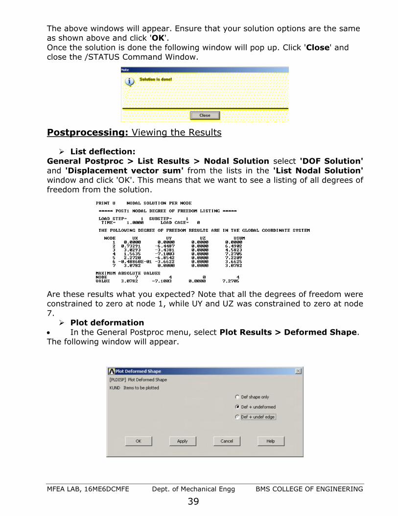
The above windows will appear. Ensure that your solution options are the same as shown above and click 'OK'.
Once the solution is done the following window will pop up. Click 'Close' and close the /STATUS Command Window.
Postprocessing: Viewing the Results
➢ List deflection: General Postproc > List Results > Nodal Solution select 'DOF Solution'
and 'Displacement vector sum' from the lists in the 'List Nodal Solution' window and click 'OK'. This means that we want to see a listing of all degrees of
freedom from the solution.
Are these results what you expected? Note that all the degrees of freedom were constrained to zero at node 1, while UY and UZ was constrained to zero at node
7. ➢ Plot deformation
• In the General Postproc menu, select Plot Results > Deformed Shape. The following window will appear.
MFEA LAB, 16ME6DCMFE Dept. of Mechanical Engg BMS COLLEGE OF ENGINEERING
40
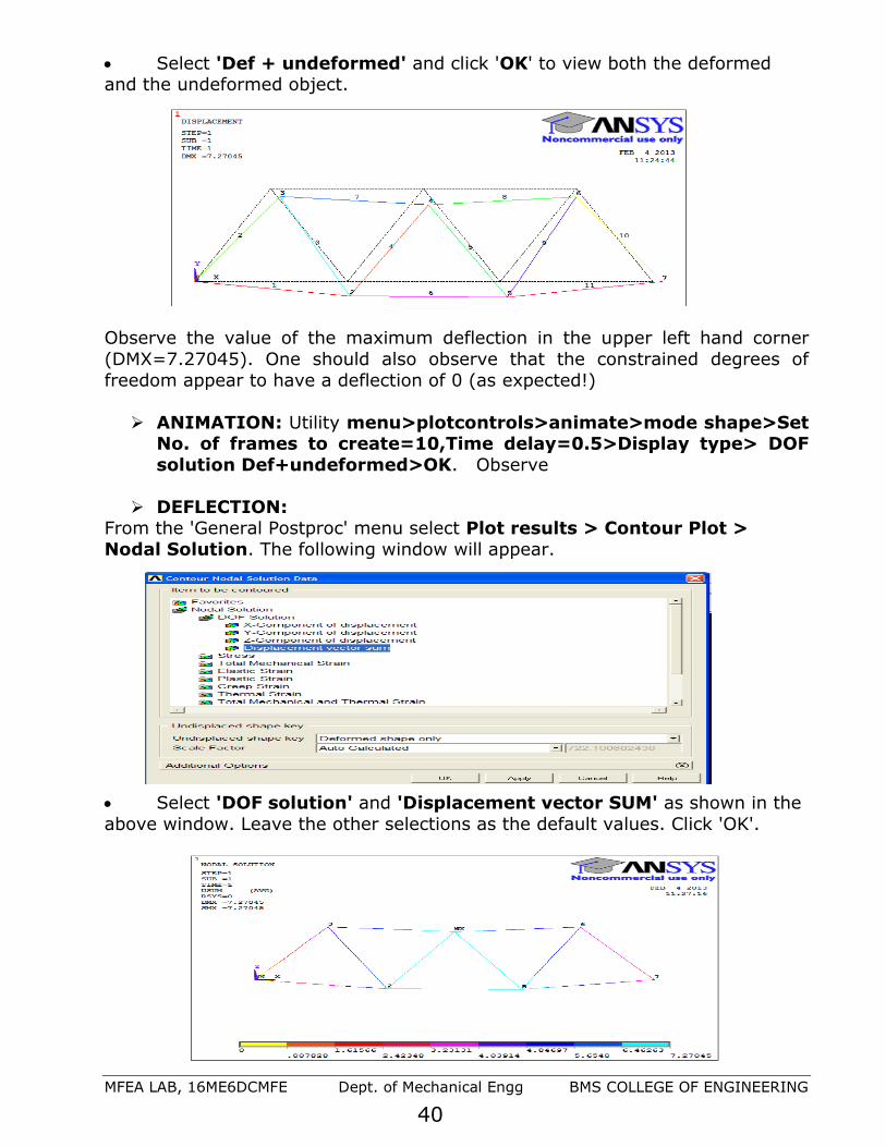
• Select 'Def + undeformed' and click 'OK' to view both the deformed and the undeformed object.
Observe the value of the maximum deflection in the upper left hand corner
(DMX=7.27045). One should also observe that the constrained degrees of
freedom appear to have a deflection of 0 (as expected!)
➢ ANIMATION: Utility menu>plotcontrols>animate>mode shape>Set No. of frames to create=10,Time delay=0.5>Display type> DOF
solution Def+undeformed>OK. Observe
➢ DEFLECTION: From the 'General Postproc' menu select Plot results > Contour Plot >
Nodal Solution. The following window will appear.
• Select 'DOF solution' and 'Displacement vector SUM' as shown in the
above window. Leave the other selections as the default values. Click 'OK'.

MFEA LAB, 16ME6DCMFE Dept. of Mechanical Engg BMS COLLEGE OF ENGINEERING
41
Looking at the scale, you may want to use more useful intervals. From the Utility Menu select Plot Controls > Style > Contours > Uniform Contours...
Fill in the following window as shown and click 'OK'.
You should obtain the following.
➢ REACTION FORCES A list of the resulting reaction forces can be obtained.
• From the Main Menu select General Postproc > List Results > Reaction Solution.
Select 'All struc forc F' as shown above and click 'OK'

MFEA LAB, 16ME6DCMFE Dept. of Mechanical Engg BMS COLLEGE OF ENGINEERING
42
Also try, From the Main Menu select General Postproc > List Results > Nodal loads. To get forces at all nodes.
➢ AXIAL STRESS (Sxx) AND FORCE(FORCE)
For line elements (i.e. links, beams, spars, and pipes) you will often need to use the Element Table to gain access to derived data (i.e. stresses, strains).
The Element Table is different for each element, therefore, we need to look at the help file for LINK180 (Type help link180 into the Input Line). From Table 5.2
we can see that Stress can be obtained through the ETABLE, using the item 'LS,1' and FORCE using ‘SMISC,1’
• From the General Postprocessor menu select Element Table > Define Table . Click on 'Add...'
As shown above, enter 'Stress' in the 'Lab' box. This specifies the name of the
item you are defining. Next, in the 'Item,Comp' boxes, select 'By sequence
number' and 'LS,'. Then enter 1 after LS, in the selection box . Click on 'Apply' and enter 'FORCE' in the 'Lab' box. This specifies the name of
the item you are defining. Next, in the 'Item,Comp' boxes, select 'By sequence number' and 'SMISC,'. Then enter 1 after SMISC, in the selection box and close
the 'Element Table Data' window.
List the Stresses • From the 'Element Table' menu, select 'List Elem Table'
• From the 'List Element Table Data' window which appears ensure 'Stress' and ‘FORCE’ are highlighted
• Click 'OK'

MFEA LAB, 16ME6DCMFE Dept. of Mechanical Engg BMS COLLEGE OF ENGINEERING
43
Plot the Stresses Element Table > Plot Elem Table
The following window will appear. Ensure that 'Stress' is selected and click 'OK'
➢ Because you changed the contour intervals for the Displacement plot to
"User Specified" - you need to switch this back to "Auto calculated" to
obtain new values for VMIN/VMAX.
Utility Menu > PlotCtrls > Style > Contours > Uniform Contours...
Again, you may wish to select more appropriate intervals for the contour plot
➢ Carryout plotting member force similarly ➢ Identify the critically loaded member.
➢ Prepare report in the format shown in the next page
Quitting ANSYS To quit ANSYS, select 'QUIT' from the ANSYS Toolbar or select Utility
Menu/File/Exit.... In the dialog box that appears, click on 'Save Everything' (assuming that you want to) and then click on 'OK'.

MFEA LAB, 16ME6DCMFE Dept. of Mechanical Engg BMS COLLEGE OF ENGINEERING
44
TRUSS- ANALYSIS REPORT Observation and tabulation
1 Node or key point number
2 Element number(Relevant real constants and material ID’s)
3 Displacement boundary conditions to be incorporated
4 Force/moment boundary conditions to be incorporated.
5 Reaction forces
6 Nodal displacements
7 Element stresses
8 Member forces
9 Maximum displacement and location
10 Maximum stress and location(Critical element)
Step1: Name and sketch the element to be used showing its degree of freedom
Ansys 3D-spar element
Sketch
Element Name:
Nodes:
Degrees of Freedom:
Real Constants:
Material Properties:.
Step2 : Sketch of the given truss structure. Show the origin and XY axes.

MFEA LAB, 16ME6DCMFE Dept. of Mechanical Engg BMS COLLEGE OF ENGINEERING
45
Step3: If geometric modeling is done, create keypoint, else node number
Keypoint/node number x y
Step4: Tabulate Cross section and material properties
Sl No. Element No. Cross section set no. and
value of side lengths in mm
Material no. and value of
E in MPa
1
Step 5: Sketch the figure showing Node number and Element number
Step 6: List
a) Displacement boundary conditions to be incorporated
Node Ux in mm Uy in mm Uz in mm
b) Force/moment boundary conditions to be incorporated
Node Fx Newton Fy Newton Fz Newton

MFEA LAB, 16ME6DCMFE Dept. of Mechanical Engg BMS COLLEGE OF ENGINEERING
46
Step 7 Results A.: NODAL SOLUTION- DISPLACEMENTS in mm
Node Ux in mm Uy in mm USUM Remark*
*Highlight node number with maximum and minimum deflection.
B: REACTION SOLUTION: in Newton
NODE FX FY FZ
Total Value
Check: Fx= Fy=
Show reaction on the truss

MFEA LAB, 16ME6DCMFE Dept. of Mechanical Engg BMS COLLEGE OF ENGINEERING
47
C: ELEMENTAL SOLUTION Specify: ETABLE Item and sequence number for Stresses LS , 1
ETABLE Item and sequence number for Member force SMISC , 1
Stresses are in MPa and Forces in N
Stat Element Current Stress Current Force
Minimum Values
Element
Values
Maximum Values
Element
Values
• Identify the element with maximum stress:
• Identify the element with maximum member force:
• Estimate the minimum Factor of safety if yield stress is 328 MPa:
• Identify the member/s which is/are yielding if the applied loads are increased 4
times:

MFEA LAB, 16ME6DCMFE Dept. of Mechanical Engg BMS COLLEGE OF ENGINEERING
48
Problem 2: Figure shows a truss with an inclined roller support at node 4. The area of cross section of the elements of the truss is 120 sq. mm. The forces acting on the nodes are shown in the figure. It is supported at node 1 by a hinged joint. Node 4 is supported on a roller arrangement and this
support allows a freedom of movement at an angle of 30. Determine the nodal displacement, reactions, and stresses in the truss member shown in figure.
:
1. File>change job name > Enter “Truss2”
2. Ansys Main Menu > Preferences > structural > Ok
3. Preprocessor > ELEMENT type > Add/edit/delete >
add > Link,3D finit stn 180> OK
4. Preprocessor > Sections > Link > Add > Add Link section with ID=1,
Section Name= ‘rect’, Area=120 > ok
5. Preprocessor > Material Properties > Material Models > Structural >
Linear > Elastic > Isotropic> EX = 2E5, PRXY = 0.3 > OK
6. Preprocessor >Modeling> Create > Nodes > In active CS >Set Node No:
= 1, X=0,Y=0, Z=0 > Apply >
Set Node No: =2, X= 2000, Y=0, Z=0 > Apply > Set Node No: =3, X= 4000, Y=0, Z=0 > Apply >
Set Node No: =4, X= 6000, Y=0, Z=0 > Apply > Set Node No: = 5, X=1000, Y=1000, Z=0 > Apply >
Set Node No: =6, X= 3000, Y=1000, Z=0 > Apply> Set Node No: =7, X= 5000, Y=1000, Z=0 > OK
NOTE: For simple line structures, mesh (Nodes and Elements) can be
directly created without geometry (without Key points and Lines).
7. Preprocessor > Modeling > Create > elements > Auto Numbered > Thru
Nodes > Pick 1 & 2 nodes > Apply > Pick 2 & 3 nodes > Apply > Pick 3 & 4 nodes > Apply > Pick 1 & 5 nodes > Apply > Pick 5 & 6 nodes > Pick 5
& 2 nodes > Apply > Pick 2 & 6 nodes > Pick 6 & 3 nodes > Apply > Pick
6 & 7 nodes > Apply > Pick 3 & 7 nodes > Apply Pick 7 & 4 nodes > OK
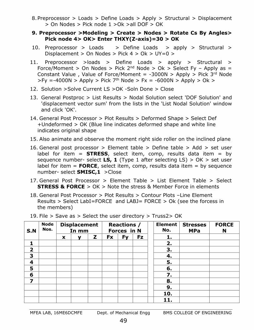
MFEA LAB, 16ME6DCMFE Dept. of Mechanical Engg BMS COLLEGE OF ENGINEERING
49
8. Preprocessor > Loads > Define Loads > Apply > Structural > Displacement
> On Nodes > Pick node 1 >Ok >all DOF > OK
9. Preprocessor >Modeling > Create > Nodes > Rotate Cs By Angles>
Pick node 4> OK> Enter THXY(Z-axis)=30 > OK
10. Preprocessor > Loads > Define Loads > apply > Structural >
Displacement > On Nodes > Pick 4 > Ok > UY=0 >
11. Preprocessor >loads > Define Loads > apply > Structural > Force/Moment > On Nodes > Pick 2nd Node > Ok > Select Fy – Apply as =
Constant Value , Value of Force/Moment = -3000N > Apply > Pick 3rd Node >Fy =-4000N > Apply > Pick 7th Node > Fx = -6000N > Apply > Ok >
12. Solution >Solve Current LS >OK -Soln Done > Close
13. General Postproc > List Results > Nodal Solution select 'DOF Solution' and
'displacement vector sum' from the lists in the 'List Nodal Solution' window
and click 'OK'.
14. General Post Processor > Plot Results > Deformed Shape > Select Def
+Undeformed > OK (Blue line indicates deformed shape and white line
indicates original shape
15. Also animate and observe the moment right side roller on the inclined plane
16. General post processor > Element table > Define table > Add > set user
label for item = STRESS, select item, comp, results data item = by sequence number- select LS, 1 (Type 1 after selecting LS) > OK > set user
label for item = FORCE, select item, comp, results data item = by sequence
number- select SMISC,1 >Close
17. General Post Processor > Element Table > List Element Table > Select
STRESS & FORCE > OK > Note the stress & Member Force in elements
18. General Post Processor > Plot Results > Contour Plots –Line Element Results > Select LabI=FORCE and LABJ= FORCE > Ok (see the forcess in
the members)
19. File > Save as > Select the user directory > Truss2> OK
S.N
Node
Nos. Displacement
In mm
Reactions /
Forces in N
Element No.
Stresses
MPa
FORCE
N
x y Z Fx Fy Fz 1.
1 2.
2 3.
3 4.
4 5.
5 6.
6 7.
7 8.
9.
10.
11.

MFEA LAB, 16ME6DCMFE Dept. of Mechanical Engg BMS COLLEGE OF ENGINEERING
50
Problem 3: Consider a two dimensional structure shown in figure 3a. The
Geometry and loading are symmetrical about the centerline. Determine nodal reactions and reactions as well as element stress and forces. A=100 mm2,
Aluminum=70x103 N/mm2, Steel =200x103 N/mm2 Use symmetry conditions (ref.fig. 3b)
➢ Ansys Main Menu > Preprocessor > Sections > Link > Add > Add Link
section with ID=1, Section Name= ‘area1’, Area=50 > Apply > Add Link
section with ID= 2, Section Name= ‘area2’, Area=100 > ok
➢ Ansys Main Menu > Preprocessor > Material Properties > Material Models
> Structural > Linear > Elastic > Isotropic> EX= 70E3, PRXY = 0.3 > OK > Material > New model > Define Material ID=2 OK > Isotropic> EX=
200E3, PRXY = 0.3 > OK > Close For Full Model: Sl
No
Node
Nos. Displacement
In mm Reactions / Forces in N
Element No.
Stresses MPa
Force N
x y Z Fx Fy Fz
1
2
3
4
For Symmetry Model: Sl
No
Node
Nos. Displacement
In mm Reactions / Forces in N
Element
No. Stresses
MPa Force
N
x y z Fx Fy Fz
1
2
3

MFEA LAB, 16ME6DCMFE Dept. of Mechanical Engg BMS COLLEGE OF ENGINEERING
51
Prioritize case a) or case b) by identifying
Sl. No. No. of
elements
used
Total no. of
DOFs in the
mesh
The size of
global stiffness
matrix
Size of modified stiffness
matrix
Elimination
approach
Penalty
approach
Case a)
Case b)
Conclusion
Problem 4: A three bar steel truss is shown in figure. All bars have the same
area of cross section of 100 mm2. If the temperature of bar 1-2 is increased by 50°C. Find the displacement of joint and the axial force in the three bars.
Young’s modulus=200Gpa, =11.7X10⁻⁶ per °C. L=1000 mm
Hint:
➢ Ansys Main Menu > Preprocessor > Material Properties > Material
Models > Structural > Linear > Elastic > Isotropic> Specify Material No:= 1> OK> Thermal expansion>secant coefficient >Isotropic> ALPX= 11.7X10⁻⁶ (and reference temperature if given, here it is not
given)> ok
➢ Ansys Main Menu > Solution >loads Define Loads > apply > Structural
>temp>on elements > pick the element at bar 1-2 > ok > Enter VAL1= rise in temp+ reference temperature if given (Enter only VAL1
for a uniform body load across the element) > ok
Sl
No
Node
Nos.
Displacement
In mm
Reaction Forces in
N
Element
No. Stress MPa
x y Z Fx Fy Fz
1 1
2 2
3 3
4
NOTE: elements between nodes 2-3 and 3-4 are not required.

MFEA LAB, 16ME6DCMFE Dept. of Mechanical Engg BMS COLLEGE OF ENGINEERING
52
Problem 5: Consider the 4 Bar Truss Shown In fig. and solve the problem for displacements stresses and Reaction Forces.
A = 100 mm2, Young’s modulus=2x10⁵ N/mm2
Results: NODAL SOLUTION- DISPLACEMENTS:
Results: REACTION SOLUTION:
Check:Fx= Fy=
Results: ELEMENTAL SOLUTION- STRESSES:
Node No. Ux Uy Uz USUM
1
2
3
4
Node No. Fx Fy Fz
1
2
3
4
Element No. Stress Force
1
2
3
4

MFEA LAB, 16ME6DCMFE Dept. of Mechanical Engg BMS COLLEGE OF ENGINEERING
53
Problem 6: Find the forces, stresses on each member of the following truss structure.
Data; A=100mm2 v= 0.3
Young’s modulus= 2e5 N/mm2.
Also find displacement field.
RESULTS:
Sl
No
Node
Nos.
Displacement
In mm
Reactions /
Forces in N
Element
No.
Stresses
MFORX
x y Z Fx Fy Fz MPa N
1 1.
2 2.
3 3.
4 4.
5 5.
6 6.
7.
8.
9.
Problem 7: For the pin-jointed configuration shown in figure. a) Calculate the reaction forces. b) Nodal displacements
c) Element stresses
Sl N
o
Node
Nos.
Displacement In mm
Reactions / Forces in N
Element
No. Stresses
MPa MFORCE
N
x y Fx Fy 1
1 2
2 3
3 4
4 5
5 6
Q2I
Q2I-1
E = 200GPa
1000 mm2
1250
mm2
P=10KN

MFEA LAB, 16ME6DCMFE Dept. of Mechanical Engg BMS COLLEGE OF ENGINEERING
54
Problem 8: For the two-bar truss shown in figure, determine the reaction forces, nodal displacements, and element stresses. If Yield stress is 400MPa,
comment on the safety of the truss structure.
Sl No
Node
Nos.
Displacement
In mm
Reactions /
Forces in N
Element
No.
Stresses
MPa
Mforce
N
x y Fx Fy
1
2
3
Problem 9: Determine the force in each member of the following truss. indicate if the member is in tension or compression. The cross-sectional area of
each member is m, the Young's modulus is 200x109 N/m2 and Poisson ratio is 0.3.
Sl
No
Node
Nos.
Displacement In mm
Reactions / Forces in N
Element
No. Stresses
MPa Mforce
N
x y Fx Fy
1
2
3
Young’s modulus = 70 GPa Area = 200 mm2 For both members

MFEA LAB, 16ME6DCMFE Dept. of Mechanical Engg BMS COLLEGE OF ENGINEERING
55
Problem 10: For the truss shown in figure, determine the reaction forces, nodal displacements, and element stresses.
A = 100 mm2, Young's modulus
= 200 GPa
Sl
No Node
Nos.
Displacement
In mm
Reactions /
Forces in N
Element
No.
Stresses MPa
x y Fx Fy
1 1
2 2
3 3
4
Problem 11: Determine the force in each member of the following truss using ANSYS. Indicate if the member is in tension or compression the cross-sectional
area of each member is 0.02 m2, Young’s modulus is 200x109 N/m2 and Poisson's ratio is 0.3.
Sl
No Node
Nos.
Displacement
In mm
Reactions / Forces in
N
Element
No.
Stresses
MPa
Force
N x y Fx Fy
1
2
3
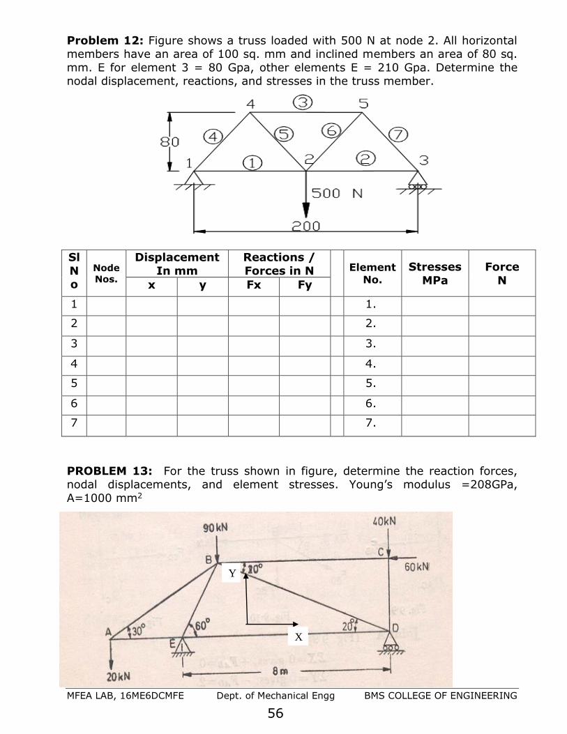
MFEA LAB, 16ME6DCMFE Dept. of Mechanical Engg BMS COLLEGE OF ENGINEERING
56
Problem 12: Figure shows a truss loaded with 500 N at node 2. All horizontal members have an area of 100 sq. mm and inclined members an area of 80 sq.
mm. E for element 3 = 80 Gpa, other elements E = 210 Gpa. Determine the nodal displacement, reactions, and stresses in the truss member.
Sl
No
Node
Nos.
Displacement
In mm
Reactions /
Forces in N
Element
No.
Stresses
MPa
Force
N x y Fx Fy
1 1.
2 2.
3 3.
4 4.
5 5.
6 6.
7 7.
PROBLEM 13: For the truss shown in figure, determine the reaction forces, nodal displacements, and element stresses. Young’s modulus =208GPa,
A=1000 mm2
X
Y
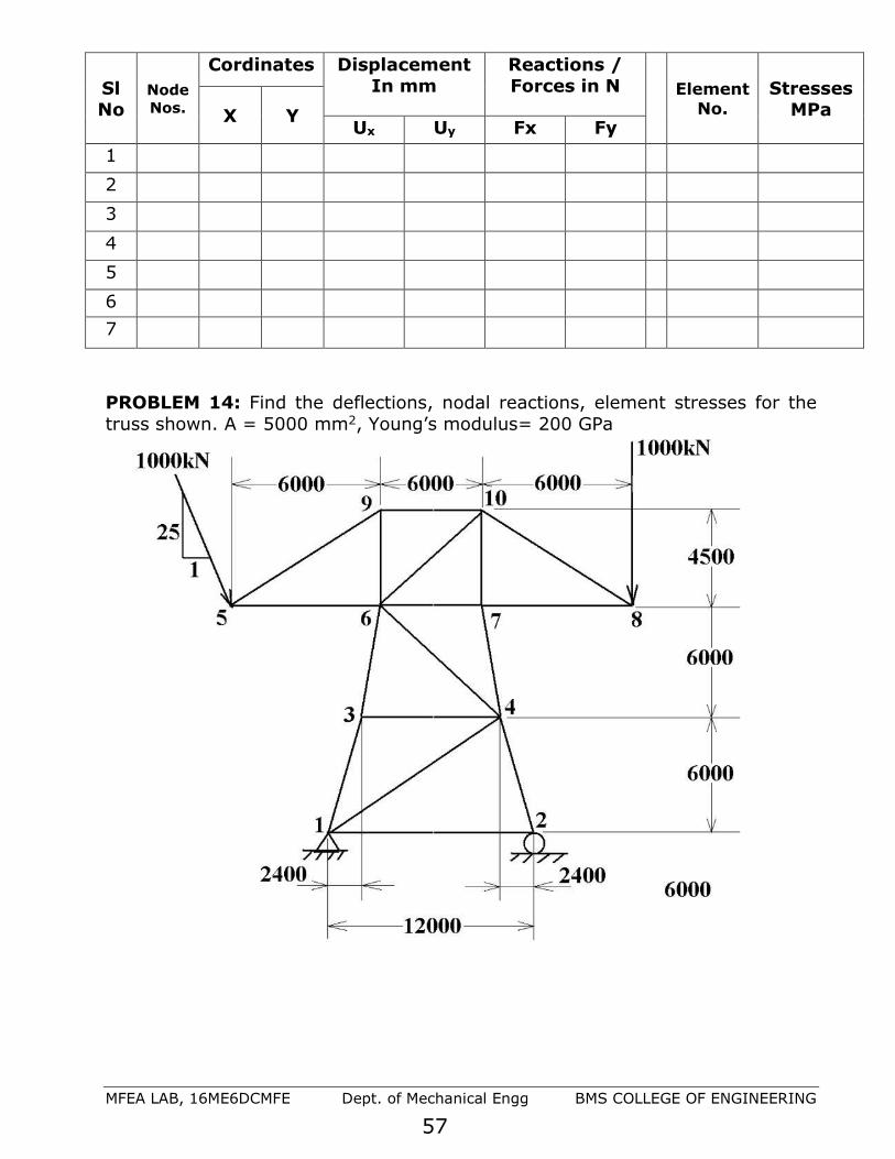
MFEA LAB, 16ME6DCMFE Dept. of Mechanical Engg BMS COLLEGE OF ENGINEERING
57
Sl No
Node
Nos.
Cordinates Displacement In mm
Reactions / Forces in N
Element
No.
Stresses MPa X Y
Ux Uy Fx Fy
1
2
3
4
5
6
7
PROBLEM 14: Find the deflections, nodal reactions, element stresses for the
truss shown. A = 5000 mm2, Young’s modulus= 200 GPa

MFEA LAB, 16ME6DCMFE Dept. of Mechanical Engg BMS COLLEGE OF ENGINEERING
58
Sl
No
Node
Nos.
Displacement In mm
Reactions / Forces in N
Element
No.
Stresses MPa
Force N
x y Fx Fy
1 1.
2 2.
3 3.
4 4.
5 5.
6 6.
7 7.
8 8.
9 9.
10 10.
11.
12.
13.
14.
15.
16.
17.

MFEA LAB, 16ME6DCMFE Dept. of Mechanical Engg BMS COLLEGE OF ENGINEERING
59
Chapter 6: PROBLEMS ON AXIAL LOADING
Problem 15: Find Nodal Displacements Stresses and reaction forces for the following problem using Link Element. AAL = 2400 mm2, Young's modulus =70x103 N/mm2, AST = 600
mm2, Young's modulus 2 =200x103 N/mm2
SOLUTION:
1. File>change job name > Enter “axial15” 2. Ansys Main Menu > Preferences > structural > Ok
3. Ansys Main Menu > Preprocessor > ELEMENT type > Add/edit/delete > add > Link,3D finit stn 180> OK
4. Ansys Main Menu > Preprocessor > Sections > Link > Add > Add Link section with ID=1, Section Name= ‘area1’, Area=2400 > Apply > Add
Link section with ID= 2, Section Name= ‘area2’, Area=600 > ok. 5. Ansys Main Menu > Preprocessor > Material Properties > Material Models
> Structural > Linear > Elastic > Isotropic> Specify Material No: = 1> OK> Young’s modulus= 70E3, Poisson’s ratio = 0.3 > apply > Specify
Material No: = 2> OK> Young’s modulus= 200E3, Poisson’s ratio= 0.3 >
apply > OK 6. Ansys Main Menu > Preprocessor >Modeling> Create > Nodes > In active
CS > Set Node No: = 1, X=0,Y=0, Z=0 > Apply > Set Node No: =2, X= 300, Y=0, Z=0 > Apply >
Set Node No: = 3, X=700, Y=0, Z=0 > OK 7. Ansys Main Menu > Preprocessor > Modeling > Create(Check Element
attributes ) > elements > Auto numbered > Thru Nodes > Pick 1 & 2 nodes > OK
8. Ansys Main Menu > Preprocessor > Modeling > Create >elements >Elements Attributes> Set Element Type No 1 LINK1,Set Material No. 2,
Set section with ID: = 2 > OK 9. Ansys Main Menu > Preprocessor > Modeling> Create> elements > Thru
Nodes> Pick nodes 2& 3 node> OK Utility menu>plot controls>style> size and shape >Display of element based
on real constant ON>ok. To visualize the stepped bar
10. Ansys Main Menu > Preprocessor > Loads > Define Loads > apply > Structural Displacement > On Nodes > Pick 1 and 3> Ok > all DOF > Ok
11. Ansys Main Menu > Preprocessor >loads > Define Loads > apply > Structural > Force/Moment > On Nodes > Pick 2nd Node > Ok > Select FX
300 mm 400 mm
200E3
Aluminium
Steel
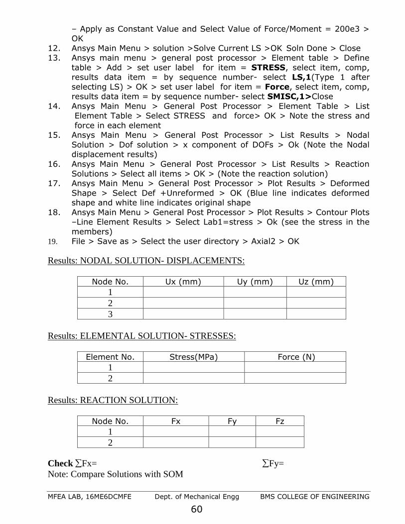
MFEA LAB, 16ME6DCMFE Dept. of Mechanical Engg BMS COLLEGE OF ENGINEERING
60
– Apply as Constant Value and Select Value of Force/Moment = 200e3 > OK
12. Ansys Main Menu > solution >Solve Current LS >OK Soln Done > Close 13. Ansys main menu > general post processor > Element table > Define
table > Add > set user label for item = STRESS, select item, comp, results data item = by sequence number- select LS,1(Type 1 after
selecting LS) > OK > set user label for item = Force, select item, comp, results data item = by sequence number- select SMISC,1>Close
14. Ansys Main Menu > General Post Processor > Element Table > List Element Table > Select STRESS and force> OK > Note the stress and
force in each element 15. Ansys Main Menu > General Post Processor > List Results > Nodal
Solution > Dof solution > x component of DOFs > Ok (Note the Nodal displacement results)
16. Ansys Main Menu > General Post Processor > List Results > Reaction
Solutions > Select all items > OK > (Note the reaction solution) 17. Ansys Main Menu > General Post Processor > Plot Results > Deformed
Shape > Select Def +Unreformed > OK (Blue line indicates deformed shape and white line indicates original shape
18. Ansys Main Menu > General Post Processor > Plot Results > Contour Plots –Line Element Results > Select Lab1=stress > Ok (see the stress in the
members) 19. File > Save as > Select the user directory > Axial2 > OK
Results: NODAL SOLUTION- DISPLACEMENTS:
Node No. Ux (mm) Uy (mm) Uz (mm)
1
2
3
Results: ELEMENTAL SOLUTION- STRESSES:
Element No. Stress(MPa) Force (N)
1
2
Results: REACTION SOLUTION:
Node No. Fx Fy Fz
1
2
Check Fx= Fy=
Note: Compare Solutions with SOM

MFEA LAB, 16ME6DCMFE Dept. of Mechanical Engg BMS COLLEGE OF ENGINEERING
61
Problem 16: case a) For the simple bar shown in the figure determine the
displacement strain, stress caused due to self-weight given length of the bar is
0.5m , cross-section area of the bar is 0.1m2 , ρ =7848 kg/m3 and Young’s Modulus 2X10¹¹ N/m2
1. File>change job name > Enter “axial16” 2. Ansys Main Menu > Preferences > structural > Ok
3. Ansys Main Menu > Preprocessor > ELEMENT type > Add/edit/delete > add > Link,3D finit stn 180> OK
4. Ansys Main Menu > Preprocessor > Sections > Link > Add > Add Link section with ID=1, Section Name= ‘area1’, Area=0.1 > ok
5. Ansys Main Menu > Preprocessor > Material Properties > Material Models
> Structural > Linear > Elastic > Isotropic> Specify Material No:= 1> OK> Youngs modulus= 2E11, Poisson’s ratio Minor= 0.3 >
OK>density>7848>ok 6. Ansys Main Menu > Preprocessor >Modeling> Create > key point > In
active CS > Set Key point No: = 1, X=0,Y=0, Z=0 > Apply > Set Key p0int NO: =2, X= 0, Y=-0.5, Z=0 > OK
7. Ansys Main Menu > Preprocessor >Modeling> Create > line > cursor pick> key points 1and 2 >Ok
8. Ansys Main Menu > Preprocessor > Meshing >Size control > Manual Size >Lines >Picked Line >NDIV=10 > OK
9. Ansys Main Menu > Preprocessor > Meshing>Mesh>Pickline> OK
10. Ansys Main Menu > Solver > loads> Define Loads > apply > Structural Displacement > On keypoint > Pick 1 > Ok > all DoF > Ok
11. Ansys Main Menu > Solver >loads> Define Loads > apply > Structural
> Inertia >Gravity>Global >ACELY=9.81>OK 12. Ansys Main Menu > solution >Solve Current LS >OK> Soln Done >
Close 13. Ansys main menu > general post processor > Element table > Define
table > Add > set user label for item = STRESS, select item, comp, results data item = by sequence number- select LS,1(Type 1 after
selecting LS) > OK > set user label for item = Force, select item, comp, results data item = by sequence number- select SMISC,1>Close
g
y

MFEA LAB, 16ME6DCMFE Dept. of Mechanical Engg BMS COLLEGE OF ENGINEERING
62
14. Ansys Main Menu > General Post Processor > Element Table > List Element Table > Select STRESS and force> OK > Note the stress and
force in each element 15. Ansys Main Menu > General Post Processor > List Results > Nodal
Solution > Dof solution > x component of DOFs > Ok (Note the Nodal displacement results)
16. Ansys Main Menu > General Post Processor > List Results > Reaction Solutions > Select all items > OK > (Note the reaction solution)
17. Ansys Main Menu > General Post Processor > Plot Results > Deformed Shape > Select Def +Unreformed > OK (Blue line indicates deformed
shape and white line indicates original shape 18. Ansys Main Menu > General Post Processor > Plot Results > Contour
Plots –Line Element Results > Select Lab1=stress > Ok (see the stress in the members)
19. File > Save as > Select the user directory > Axial 16> OK Results: SOLUTION- DISPLACEMENTS: Element solution
Node No. Ux
(mm)
Uy
(mm)
Uz
(mm)
Element Stress
(MPa)
Force
N
1.
2.
3.
4.
5.
6.
7.
8.
9.
10.
11.
Results: REACTION SOLUTION:
Node No. Fx Fy
1
Check Fx= Fy=
Compare with SOM Solutions
E
glxu x
2
= ==
E
glu
2
2
max
Problem 16: case b) Solve the same problem by putting total weight at free end
and Compare:

MFEA LAB, 16ME6DCMFE Dept. of Mechanical Engg BMS COLLEGE OF ENGINEERING
63
Problem 17: Model the figure with 1D bar elements and find tip
displacement. Carry out convergence study (H - convergence) by increasing the
number of elements (1,2,4,8) and plot graph of displacement Vs number of elements and Compare with theoretical value.
P = 10kN, d1 = 40 mm, d2 = 20 mm, l = 300 mm,
Young's modulus = 20 Gpa
Note: For Taper rod under axial loading, Theoretical deflection
=4Pl /( Ed1d2)
STEP 1 One element
RC= * 302/4=706.85 mm2, Le=300 mm
20
1515
30
1 2
1
40
Displacements In mm
NODE UX UY UZ USUM
1 0.0000 0.0000 0.0000 0.0000
2 0.21221 0.0000 0.0000 0.21221
MAXIMUM ABSOLUTE VALUES NODE 2 0.21221
ELEMENT STRESSES (LS,1)
ELEM STRESS (MPa)
1 14.147

MFEA LAB, 16ME6DCMFE Dept. of Mechanical Engg BMS COLLEGE OF ENGINEERING
64
STEP 2 Two elements
RC-1= * 352/4=962.113 mm2, Le=150 mm
RC-2= * 252/4=490.873 mm2 Le=150 mm
20
1
40
3
RC-1 RC-2
21 2
2535
Nodes and coordinates
NODE X Y
1 0.0000 0.0000
2 150.00 0.0000
3 300.00 0.0000
Connectivity table
ELEM NODES AREA mm2 MAT
1 1 2 962.113 1
2 2 3 490.873 1
Displacements in mm
NODE UX UY UZ USUM
1 0.0000 0.0000 0.0000 0.0000
2 0.77953E-01 0.0000 0.0000 0.77953E-01
3 0.23074 0.0000 0.0000 0.23074
MAXIMUM ABSOLUTE VALUES
NODE3 0.23074
ELEMENT STRESSES (LS 1) in MPa
ELEM STRESS
1 10.394
2 20.372
STEP 3 Four elements
RC-1= * 37.52/4=1105.64 mm2, Le=75 mm
RC-2= * 32.52/4=829.577 mm2 Le=75 mm
RC-3= * 27.52/4=593.95 mm2, Le=75 mm
RC-4= * 22.52/4=397.6 mm2 Le=75 mm

MFEA LAB, 16ME6DCMFE Dept. of Mechanical Engg BMS COLLEGE OF ENGINEERING
65
20
1
40
3
RC-1 RC-2
4
RC-3 RC-4
2 51 2 3 4
37,5
32,5
27,5
22,5
Nodes and coordinates
NODE X Y Z THXY THYZ THZX
1 0.0000 0.0000 0.0000 0.00 0.00 0.00
2 75.000 0.0000 0.0000 0.00 0.00 0.00
3 150.00 0.0000 0.0000 0.00 0.00 0.00
4 225.00 0.0000 0.0000 0.00 0.00 0.00
5 300.00 0.0000 0.0000 0.00 0.00 0.00
LIST ALL SELECTED ELEMENTS.
ELEM NODES AREA mm2 MAT
1 1 2 1105.63 1
2 2 3 829.566 1
3 3 4 593.957 1
4 4 5 397.61 1
Displacements In mm
NODE UX UY UZ USUM 1 0.0000 0.0000 0.0000 0.0000
2 0.33917E-01 0.0000 0.0000 0.33917E-01
3 0.79121E-01 0.0000 0.0000 0.79121E-01
4 0.14226 0.0000 0.0000 0.14226
5 0.23657 0.0000 0.0000 0.23657
ELEMENT STRESSES (LS 1)in MPa
STAT CURRENT
ELEM STRESS
1 9.0445
2 12.054
3 16.836
4 25.151
CONVERGENCE STUDIES-H CONVERGENCE
SL.NO NUMBER
OF
ELEMNTS
TIP
DISPLCEMENT(ANSYS)
IN mm
TIP
DISPLCEMENT
EXACT FROM
SOM
In mm
Stress at
small(Free)
end(ANSYS)
MPa
Stress at small(Free)
end
MPa
1 1 0.21221 exact =4PL
E d1d2
= 0.2387314
14.147 =4p/(d22)
=31.85 2 2 0.23074 20.372
3 4 0.23657 25.151

MFEA LAB, 16ME6DCMFE Dept. of Mechanical Engg BMS COLLEGE OF ENGINEERING
66
Convergence of Tip Displacement with increase in
Number of Elements
0.21
0.215
0.22
0.225
0.23
0.235
0.24
0.245
0 1 2 3 4 5
No.of Elements
Tip
Dis
pla
cem
ent
Graph of H Convergence
Graph of Convergence of tip stress with increase in number of elements
Question: Check whether displacement or stress converges faster. What are its implications?

MFEA LAB, 16ME6DCMFE Dept. of Mechanical Engg BMS COLLEGE OF ENGINEERING
67
D1 = (d1+d2) / 2
d3 = (d1+d2) / 2 D1 = (d1+d3) / 2 D2 = (d3+d2) / 2
Problem18: Model the figure with 1D bar elements and find tip displacement
carry out convergence study (H - convergence) by increasing the number of
elements (1,2,4,8) and plot graph of Vtip displacement Vs number of elements and Compare with theoretical value. P = 15kN, t = 15 mm, d1 = 100 mm, d2
= 40 mm, l = 300mm, Young’s modulus E = 200 Gpa, poison's ratio = 0.3
Theoretical deflection = {Pl loge(d1/d2)}/ {E t (d1-d2)} ELEMENT TYPE =
No. of elements: One
Displacement ux at node 2 = A1 = D1.t = No. of elements : Two Discretization (connectivity) and material properties
Displacement ux at node 3 =
Sl. No. Element No.
Node No.
Length mm
C/S area E (Gpa)
1 1-2
2 2-3

MFEA LAB, 16ME6DCMFE Dept. of Mechanical Engg BMS COLLEGE OF ENGINEERING
68
No. of elements : Four Discretisation (connectivity) and material properties
Sl. No. Element No.
Node No.
Length C/S area
1 1 1-2
2 2 2-3
3 3 3-4
4 4 4-5
Displacement ux at node 5 = No. of elements: eight Discretization (connectivity) and material properties
Sl. No. Element No.
Node No.
d1 mm
d2 mm
Length mm
C/S
D, mm A, mm2
1 1 1-2
2 2 2-3
3 3 3-4
4 4 4-5
5 5 5-6
6 6 6-7
7 7 7-8
8 8 8-9

MFEA LAB, 16ME6DCMFE Dept. of Mechanical Engg BMS COLLEGE OF ENGINEERING
69
Answer - Tip deflection
Theoretical No. of Finite Elements
1 2 4 8
Convergence of Tip Displacement with increase in
Number of Elements
0
0.05
0.1
0.15
0.2
0.25
0.3
0.35
0.4
0.45
0 1 2 3 4 5
No.of Elements
Tip
Dis
plac
emen
t
Graph of H Convergence
Graph of Convergence of tip stress with increase in number of elements

MFEA LAB, 16ME6DCMFE Dept. of Mechanical Engg BMS COLLEGE OF ENGINEERING
70
Problem 19: A copper bar of Length 160mm is placed on rigid support in vertical
position .Clearance between the upper support and top surface of the member is 0.1mm as shown. Determine Stress and reactions for 1) when the temperature is raised by 34.70C. 2) when the temperature is raised by 810C. 3) when the temperature is raised by 900C and upper support yields by 0.12mm and 4) when the temperature is raised by 300C and there
is no clearance between upper support and top surface of the bar. E c=120 GPa and =
18 x 10-6 per C. A=10mm2
Note:
➢ Ansys Main Menu > Preprocessor > Material Properties > Material
Models > Structural > Linear > Elastic > Isotropic> Specify Material No:= 1> OK> Thermal expansion>secant coefficient >Isotropic>
ALPX= 18 e-6
(and reference temperature if given)> ok
➢ Ansys Main Menu > Solver >loads Define Loads > apply > Structural
>temp>uniform temp=(rise in temp+ reference temperature if given)> ok
Case Description Force-N Stress in
MPa -Ansys Stress in MPa
SOM
1.
2.
3.
4.

MFEA LAB, 16ME6DCMFE Dept. of Mechanical Engg BMS COLLEGE OF ENGINEERING
71
Problem 20: Find Nodal Displacements Stresses and reaction forces for the following problem using Link1 Element. Given data: A1 = 40mm2,
A2 = 20mm2, Young's modulus =2x10⁵ N/mm2
Results: NODAL SOLUTION- DISPLACEMENTS:
Node No. Ux (mm) Uy (mm)
1
2
3
Results: ELEMENTAL SOLUTION- STRESSES:
Element No. Stress(MPa) Force (N)
1
2
Results: REACTION SOLUTION:
Node No. Fx Fy
1
2
Check Fx= Fy=
Note:Compare Solutions with SOM
A2=20mm2
40 mm 20 mm
A1= 40mm2
1000N

MFEA LAB, 16ME6DCMFE Dept. of Mechanical Engg BMS COLLEGE OF ENGINEERING
72
Problem21: Consider the bar shown in figure. An axial load p=200 x 103 N is applied as shown. Determine 1) the nodal displacements and the reaction forces & 2) Element
stresses. Area1 = 2400 mm2 Area 2= 600 mm2
Young's modulus = 70 x 109 N/m2 Young's modulus = 200 x 109 N/m2 Descretization (connectivity) and material properties
Sl. No. Element No.
Node Nos.
Length C/S
E (Gpa)
1
2
Answer
Sl. No. Node No. Deflection. mm
Load / Reaction N
Element No Stress MPa Force (N)
1 ➢
2 ➢
3
Check R1+R3+P = 0

MFEA LAB, 16ME6DCMFE Dept. of Mechanical Engg BMS COLLEGE OF ENGINEERING
73
Problem 22: Determine the displacement field, support reactions & stress in the
body shown as loaded. Use 1D bar elements.
Young's modulus = 20 Gpa A = 250 mm2 P = 60 kN Case A Case B & C Also what will be these values for case B
and Case C
Case B : g =1.2 mm Case C : g = 2 mm Answer Sl. No
Node No.
CASE A CASE B CASE C
Displacement mm
Reaction N
Displacement mm
Reaction N
Displacement mm
Reaction N
1
2
3
Stresses in element MPa
1 2
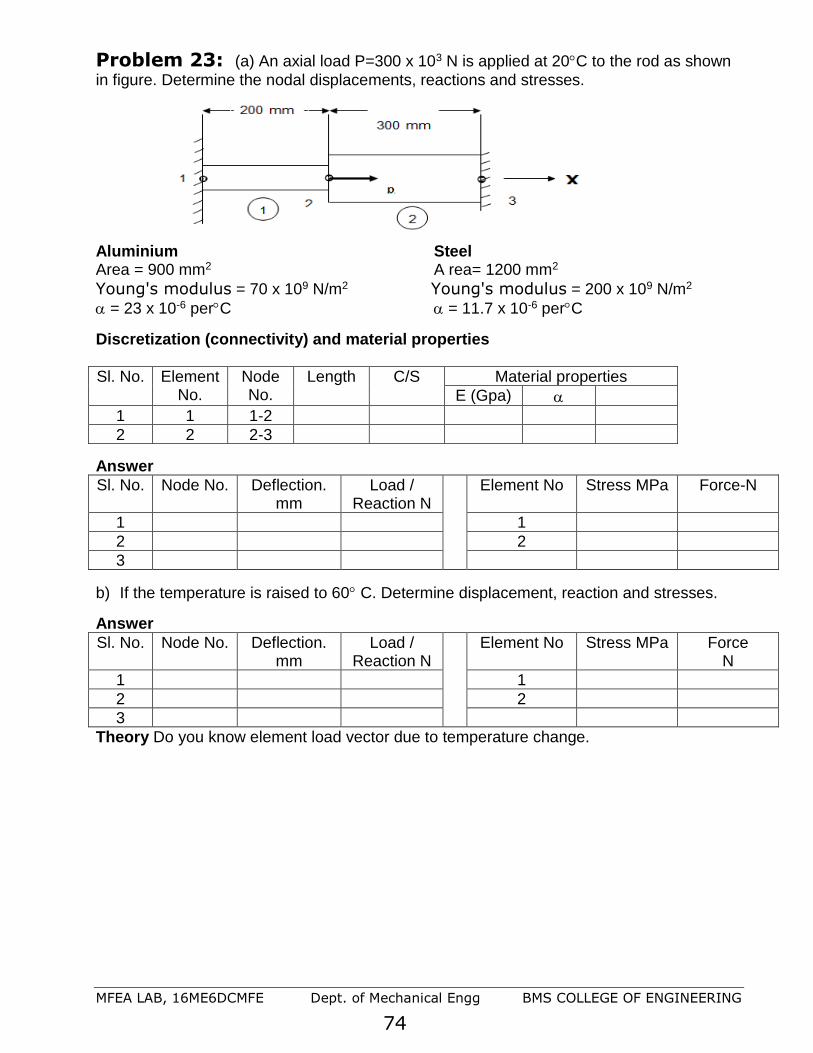
MFEA LAB, 16ME6DCMFE Dept. of Mechanical Engg BMS COLLEGE OF ENGINEERING
74
Problem 23: (a) An axial load P=300 x 103 N is applied at 20C to the rod as shown
in figure. Determine the nodal displacements, reactions and stresses.
Aluminium Steel Area = 900 mm2 A rea= 1200 mm2
Young's modulus = 70 x 109 N/m2 Young's modulus = 200 x 109 N/m2
= 23 x 10-6 perC = 11.7 x 10⁻⁶ perC
Discretization (connectivity) and material properties
Sl. No. Element No.
Node No.
Length C/S Material properties
E (Gpa)
1 1 1-2
2 2 2-3
Answer
Sl. No. Node No. Deflection. mm
Load / Reaction N
Element No Stress MPa Force-N
1 1
2 2
3
b) If the temperature is raised to 60 C. Determine displacement, reaction and stresses.
Answer
Sl. No. Node No. Deflection. mm
Load / Reaction N
Element No Stress MPa Force N
1 1
2 2
3
Theory Do you know element load vector due to temperature change.
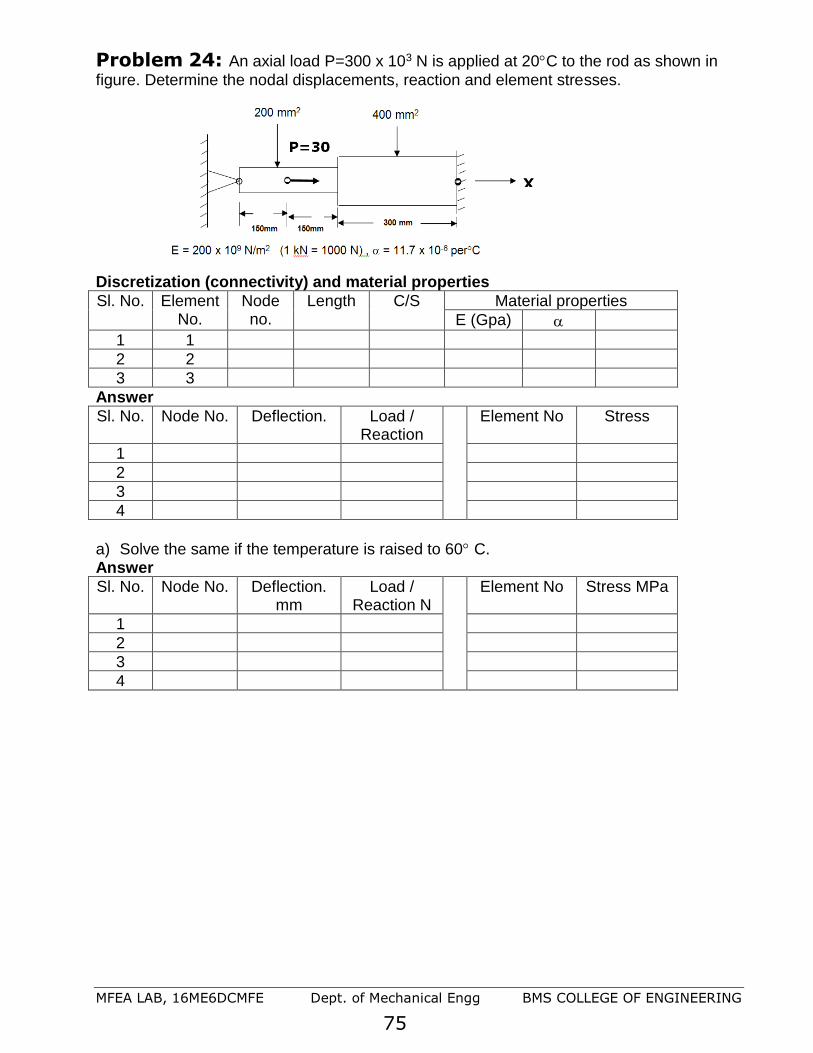
MFEA LAB, 16ME6DCMFE Dept. of Mechanical Engg BMS COLLEGE OF ENGINEERING
75
Problem 24: An axial load P=300 x 103 N is applied at 20C to the rod as shown in
figure. Determine the nodal displacements, reaction and element stresses. Discretization (connectivity) and material properties
Sl. No. Element No.
Node no.
Length C/S Material properties
E (Gpa)
1 1
2 2
3 3
Answer
Sl. No. Node No. Deflection. Load / Reaction
Element No Stress
1
2
3
4
a) Solve the same if the temperature is raised to 60 C. Answer
Sl. No. Node No. Deflection. mm
Load / Reaction N
Element No Stress MPa
1
2
3
4

MFEA LAB, 16ME6DCMFE Dept. of Mechanical Engg BMS COLLEGE OF ENGINEERING
76
Problem 25: Consider the bar in figure. Determine the nodal displacements, element
stresses and support reactions. a) At room temperature b) The temperature is then
raised to 60C
= 11.7 x 10⁻⁶ perC Young's modulus = 200 x 109 N/m2 , Discretization (connectivity) and material properties
Sl. No. Element No.
No. of nodes
Length C/S Material properties
E (Gpa)
1
2
3
4
Answer: Part A
Sl. No. Node No. Deflection. mm
Load / Reaction N
Element No Stress MPa
1
2
3
4
5
Answer:Part B
Sl. No. Node No. Deflection. mm
Load / Reaction N
Element No Stress MPa
1
2
3
4
5

MFEA LAB, 16ME6DCMFE Dept. of Mechanical Engg BMS COLLEGE OF ENGINEERING
77
Problem 26: For the structure shown
Case a-without temperature rise , Case b-with temperature rise of 80oC 1) Specify the type of element to be used. 2) Create finite element model showing element numbers & node numbers. 3) Specify the displacement and force boundary condition s 4) Obtain nodal reaction s. 5) Displacement of various nodes. Identify maximum displacement with location 6) Stresses and force along each element.
Bronze Aluminium Steel A = 2400 mm2 A = 1200 mm2 A = 600 mm2 E = 83 GPa E = 70 GPa E = 200 GPa
= 18.9 x 10⁻⁶ perC = 23 x 10-6 perC = 11.7 x 10⁻⁶ perC STEP1 NODE NUMBERING AND COORDINATES
NODE X Y
1 0.0000 0.0000
2 800.00 0.0000
3 1400.0 0.0000
4 1800.0 0.0000
STEP2 LIST ALL SELECTED ELEMENTS.
ELEM NODES Real Constant AREA (mm2) MAT ID E-MPa /0C
1 1,2 1 2400.00 1 83e3 18.9e-6
2 2,3 2 1200.00 2 70e3 23e-6
3 3,4 3 600.000 3 200e3 11.7e-6
STEP3 CURRENTLY SELECTED DOF SET= UX UY
NODE LABEL REAL
1 UX 0.00000000
1 UY 0.00000000
4 UX 0.00000000
4 UY 0.00000000
STEP 4 LIST NODAL FORCES FOR SELECTED NODES in Newton
NODE LABEL REAL
2 FX -60000.0000
3 FX -75000.0000

MFEA LAB, 16ME6DCMFE Dept. of Mechanical Engg BMS COLLEGE OF ENGINEERING
78
RESULTS PARTICULAR CASE A WITHOUT TEMPERATURE CASE B WITH TEMPERATURE RISE of
80 deg.C
Displacements
In mm
NODE UX USUM
1 0.0000 0.0000
2 -0.24347 0.24347
3 -0.24792 0.24792
4 0.0000 0.0000
MAXIMUM ABSOLUTE VALUES
NODE 2
VALUE -0.24792
NODE UX USUM
1 0.0000 0.0000
2 0.22124 0.22124
3 -0.40603E-02 0.40603E-02
4 0.0000 0.0000
MAXIMUM ABSOLUTE VALUES
NODE 2
VALUE 0.22124
REACTION IN
NEWTON
NODE FX FY
1 60624. 0.0000
4 74376. 0.0000
TOTAL VALUES
VALUE 0.13500E+06 0.0000
NODE FX FY
1 0.24610E+06 0.0000
4 -0.11110E+06 0.0000
TOTAL VALUES
VALUE 0.13500E+06 0.0000
ELEMENT
STRESSES
(LS,1) &
MEMBER FORCE
(SMISC,1)
FROM ETABLE
ELEM STRESS FORCE
(MPA) (NEWTON)
1 -25.260 -60624.
2 -0.51960 -623.52
3 123.96 74376.
MINIMUM VALUES
ELEM 1 1
VALUE -25.260 -60624.
MAXIMUM VALUES
ELEM 3 3
VALUE 123.96 74376.
ELEM STRESS FORCE
(MPA) (NEWTON)
1 -102.54 -0.24610E+06
2 -155.08 -0.18610E+06
3 -185.17 -0.11110E+06
MINIMUM VALUES
ELEM 3 1
VALUE -185.17 -0.24610E+06
MAXIMUM VALUES
ELEM 1 3
VALUE -102.54 -0.11110E+06

MFEA LAB, 16ME6DCMFE Dept. of Mechanical Engg BMS COLLEGE OF ENGINEERING
79
Problem 27: Three equidistant vertical rods, each of 20mm dia, support a load as
shown taking Es=205GPa and Ec=100GPa determine the final stresses
Given Data: Ls=3.6m,
Lc=2.8m,
d=20mm
Hint : Horizontal bar remains horizontal. Hence the upper ends of all the vertical bars move together vertically. So we need to couple them in Uy. Assume a=1000mm.
Procedure Ansys Main Menu > Preferences > Structural > Ok
Ansys Main Menu > Preprocessor > Element type > Add/edit/delete > add >LINK > 3D Finite Stn>
OK > close Ansys Main Menu > Preprocessor > Sections > Link > Add > Add Link section with ID=1, Section Name= ‘area1’, Area=3.142*20**2/4 > ok Ansys Main Menu > Preprocessor > Material Properties > Material Models > Structural > Linear >
Elastic >Isotropic> EX= 205E3, PRXY= 0.3, OK> Material>New Model> Specify Material No: =
2> OK> EX= 100E3, PRXY= 0.3, OK
Ansys Main Menu > Preprocessor >Modeling> Create > Nodes > in active CS >
Set Node No: = 1, X=0, Y=0, Z=0 > Apply > Set Node No: =2, X= 0, Y=3600, Z=0 > Apply >
Set Node No: =3, X= 1000, Y=800, Z=0 > Apply > Set Node No: =4, X= 1000, Y=3600, Z=0 >
Apply >Set Node No: =5, X= 2000, Y=0, Z=0 >Apply > set Node No:=6, X= 2000, Y = 3600, Z=0
>OK
Ansys Main Menu > Preprocessor > Modeling > Create > elements > Element Attributes > Material
no. = 1, Real constant set no. = 1 > ok
Ansys Main Menu > Preprocessor > Modeling > Create > elements > Auto numbered > Thru Nodes
> Pick nodes 1 and 2 > Apply > pick nodes 5 and 6 > ok
Ansys Main Menu > Preprocessor > Modeling > Create > elements > Element Attributes > Material
no. = 2, Real constant set no. = 1 > ok
Ansys Main Menu > Preprocessor > Modeling > Create > elements > Auto numbered > Thru Nodes
> Pick nodes 3 and 4 > ok
Ansys Main Menu > Preprocessor > Coupling/Ceqn > Couple DOFs > pick nodes 2, 4 and 6, ok >
set reference no. = 1, Degree of freedom label = Uy > ok
Ansys Main Menu > Preprocessor > Loads > Define Loads > Apply > Structural > Displacement >
On Nodes > Pick nodes 1, 3 and 5, Ok> DOFs to be constrained= All DOF, ok.
25kN
a a
2.8
m
3.6
m
ST
EE
L
CO
PP
ER
ST
EL
L

MFEA LAB, 16ME6DCMFE Dept. of Mechanical Engg BMS COLLEGE OF ENGINEERING
80
Ansys Main Menu > Preprocessor >loads > Define Loads > apply > Structural >Force/Moment > On
Nodes > Pick node 4 > Ok > Select Fy= –25e3, ok
Ansys Main Menu > solution >Solve Current LS >OK
Ansys main menu > general post processor > Element table > Define table > Add > set user label for
item = STRESS, select item, comp, results data item = by sequence number- select LS, 1 (Type 1
after selecting LS) > OK > set user label for item = FORCE, select item, comp, results data item =
by sequence number- select SMISC,1>Close
Ansys Main Menu > General Post Processor > Element Table > List Element Table > Select
STRESS & FORCE > OK > Note the stress & Force in elements
Ansys Main Menu > General Post Processor > List Results > Nodal Solution >Dof solution > x
component of DOFs > Ok (Note the Nodal displacement results)
Ansys Main Menu > General Post Processor > List Results > Reaction Solutions > Select all items >
OK > (Note the reaction solution) RESULTS: Results: NODAL SOLUTION- DISPLACEMENTS:
Node No. Ux (mm) Uy (mm) Uz(mm)
1
2
3
Results: ELEMENTAL SOLUTION- STRESSES:
Element No. Stress(MPa) Force (N)
1
2
3
Results: REACTION SOLUTION:
Node No. Fx Fy Fz
1
2
3

MFEA LAB, 16ME6DCMFE Dept. of Mechanical Engg BMS COLLEGE OF ENGINEERING
81
Problem 28: Three equally spaced rods in the same vertical are Brasses, each 600mm long and of 25mm in dia, The central rod is of steel that is 800mm long and 30mm in dia, determine the forces in each rods due to an applied load of 120kN downwards through the midpoint of the bar, The bar remains horizontal after the application of load. Take
Es=200GPA and Eb=105GPa.
RESULTS :
Results: NODAL SOLUTION- DISPLACEMENTS:
Node No. Ux (mm) Uy (mm) Uz(mm)
1
2
3
Results: ELEMENTAL SOLUTION- STRESSES:
Element No. Stress(MPa) Force (N)
1
2
3
Results: REACTION SOLUTION:
Node No. Fx Fy Fz
1
2
3
BR
AS
S
a a
600 m
m
800 m
m
ST
EE
L
BR
AS
S
Ø 25mm
Ø 30mm

MFEA LAB, 16ME6DCMFE Dept. of Mechanical Engg BMS COLLEGE OF ENGINEERING
82
Problem 29: A rigid horizontal bar AB hinged at A is supported by a 1.2m long steel rod and a 2.4m long bronze rod, both rigidly fixed at the upper ends, A load of 48kN is applied at a point that is 3.2m from the hinge point A, the areas of cross-section of steel and bronze rods are 850mm2 and 650mm2 respectively. Find stress in each rod.
Given Data:
As=850mm2 Ab=650mm2
Es=205GPa Eb=82GPA
Hint : Model AB with three MPC184 elements(constraint element) with ‘Rigid
beam’ element option. Allow Rotz DOF for node at A.
Procedure Ansys Main Menu > Preferences > Structural > Ok
Ansys Main Menu > Preprocessor > ELEMENT type > Add/edit/delete > add >LINK > 3D Finite
Stn> OK
Ansys Main Menu > Preprocessor > ELEMENT type > Add/edit/delete > add >Constraint >Non
linear MPC184>OK>Options>K1 Rigid Beam>K2 Lagrange Multiplier>OK
Ansys Main Menu > Preprocessor > Sections > Link > Add > Add Link section with ID=1, Section
Name= ‘area1’, Area=850 > Apply > Add Link section with ID= 2, Section Name= ‘area2’,
Area=650 > ok.
Ansys Main Menu > Preprocessor > Material Properties > Material Models > Structural > Linear >
Elastic >Isotropic> EXX= 205E3, PRXY= 0.3, OK> Material>New Model> Specify Material No: =
2> OK> EXX= 82E3, PRXY= 0.3, OK
Ansys Main Menu > Preprocessor >Modeling> Create > Nodes > in active CS >
Set Node No: = 1, X=0, Y=0, Z=0 > Apply > Set Node No: =2, X= 800, Y=0, Z=0 > Apply >
Set Node No: =3, X= 800, Y=1200, Z=0 > Apply > Set Node No: =4, X= 2400, Y=0, Z=0 > Apply
>Set Node No: =5, X= 2400, Y=2400, Z=0 >Apply > set Node No:=6, X= 3200, Y = 0, Z=0 >OK
Ansys Main Menu > Preprocessor > Modeling > Create (Check Element attributes) > elements >
Auto numbered > Thru Nodes > Pick 2&3 nodes > OK
Ansys Main Menu > Preprocessor > Modeling > Create >elements >Elements Attributes> Set
Element Type No 1 LINK1, Set Material No. 2, Set real constant set No: = 2> OK
Ansys Main Menu > Preprocessor > Modeling> Create> elements> Thru Nodes> Pick nodes 4&5
node> OK
Ansys Main Menu > Preprocessor > Modeling > Create >elements >Elements Attributes> Set
Element Type No 1MPC184, > OK

MFEA LAB, 16ME6DCMFE Dept. of Mechanical Engg BMS COLLEGE OF ENGINEERING
83
Ansys Main Menu > Preprocessor > Modeling> Create> elements> Thru Nodes> Pick nodes
1&2,2&4, and 4&6> OK
Ansys Main Menu > Preprocessor > Loads > Define Loads > apply > Structural Displacement > On
Nodes > Pick 1 Ok >Select UX,UY,UZ,ROTX,ROTY> Ok
Ansys Main Menu > Preprocessor > Loads > Define Loads > apply > Structural Displacement > On
Nodes > Pick 3 &5 Ok>Select All Dof> Ok
Ansys Main Menu > Preprocessor >loads > Define Loads > apply > Structural >Force/Moment > On
Nodes > Pick 6th Node > Ok > Select Fy= –48000
Ansys Main Menu > solution >Solve Current LS >OK Soln Done > Close
Ansys main menu > general post processor > Element table > Define table > Add > set user label for
item = STRESS, select item, comp, results data item = by sequence number- select LS, 1 (Type 1
after selecting LS) > OK > set user label for item = FORCE, select item, comp, results data item =
by sequence number- select SMISC,1>Close
Ansys Main Menu > General Post Processor > Element Table > List Element Table > Select
STRESS & FORCE > OK > Note the stress & Force in elements
Ansys Main Menu > General Post Processor > List Results > Nodal Solution >Dof solution > x
component of DOFs > Ok (Note the Nodal displacement results)
Ansys Main Menu > General Post Processor > List Results > Reaction Solutions > Select all items >
OK > (Note the reaction solution)
RESULTS: Results: NODAL SOLUTION- DISPLACEMENTS:
Node No. Ux (mm) Uy (mm) Uz (mm)
1
2
3
4
5
6
Results: ELEMENTAL SOLUTION- STRESSES:
Element No. Stress(MPa) Force (N)
_ _ (Steel)
_ _ (Bronze)
Results: REACTION SOLUTION:
Node No. Fx Fy Fz
1
3
5

MFEA LAB, 16ME6DCMFE Dept. of Mechanical Engg BMS COLLEGE OF ENGINEERING
84
Chapter7: Problems on Beams
3-D 2-Node Beam (beam188, beam189) geometry
Fig.7.1
Element Description:
BEAM188 is suitable for analyzing slender to moderately stubby/thick beam structures. The element is based on Timoshenko beam theory which includes shear-deformation effects. The element provides options for unrestrained warping and restrained warping of cross-sections.
The element is a linear, quadratic, or cubic two-node beam element in 3-D. BEAM188 has six or seven degrees of freedom at each node. These include translations in the x, y, and z directions and rotations about the x, y, and z directions. A seventh degree of freedom (warping magnitude) is optional. This element is well-suited for linear, large rotation, and/or large strain nonlinear applications.
The element includes stress stiffness terms, by default, in any analysis with large deflection. The provided stress-stiffness terms enable the elements to analyze flexural, lateral, and torsional stability problems (using eigenvalue buckling, or collapse studies with arc length methods or nonlinear stabilization).
Elasticity, plasticity, creep and other nonlinear material models are supported. A cross-section associated with this element type can be a built-up section referencing more than one material.
Assumptions and Restrictions:
• The beam must not have zero length. • By default (KEYOPT(1) = 0), the effect of warping restraint is assumed to be
negligible. • Cross-section failure or folding is not accounted for. • Rotational degrees of freedom are not included in the lumped mass matrix if offsets
are present. • The element works best with the full Newton-Raphson solution scheme (that is, the
default choice in solution control).

MFEA LAB, 16ME6DCMFE Dept. of Mechanical Engg BMS COLLEGE OF ENGINEERING
85
• Only moderately "thick" beams can be analyzed. See "BEAM188 Element Technology and Usage Recommendations" for more information.
• Stress stiffening is always included in geometrically nonlinear analyses (NLGEOM,ON). Prestress effects can be activated by the PSTRES command.
• When the element is associated with nonlinear general beam sections (SECTYPE,,GENB), additional restrictions apply. For more information, see Considerations for Using Nonlinear General Beam Sections.
• The element coordinate system (/PSYMB,ESYS) is not relevant. • For a random vibration (PSD) analysis, equivalent stress is not calculated.
BEAM188 Input Data:
The geometry, node locations, coordinate system, and pressure directions for this element are shown in Figure 7.1. BEAM188 is defined by nodes I and J in the global coordinate system.
Node K is a preferred way to define the orientation of the element. For information about orientation nodes and beam meshing, see Generating a Beam Mesh With Orientation Nodes in the Modeling and Meshing Guide. See the LMESH and LATT command descriptions for details on generating the K node automatically.
BEAM188 can also be defined without the orientation node K. In this case, the element x-axis is oriented from node I (end 1) toward node J (end 2). If no orientation node is used, the default orientation of the element y-axis is automatically calculated to be parallel to the global X-Y plane. For the case where the element is parallel to the global Z-axis (or within a 0.01 percent slope of it), the element y-axis is oriented parallel to the global Y-axis (as shown). To control the element orientation about the element x-axis, use the orientation-node option. If both are defined, the orientation-node option takes precedence. The orientation node K, if used, defines a plane (with I and J) containing the element x and z-axes (as shown). If using this element in a large-deflection analysis, be aware that the location of the orientation node K is used only to initially orient the element.
The number of degrees of freedom depends on the value of KEYOPT(1). When KEYOPT(1) = 0 (the default), six degrees of freedom occur at each node. These include translations in the x, y, and z directions and rotations about the x, y, and z directions. When KEYOPT(1) = 1, a seventh degree of freedom (warping magnitude) is also considered.
The beam element is a one-dimensional line element in space. The cross-section details are provided separately via the SECTYPE and SECDATA commands. (See Beam Analysis and cross-sections in the Structural Analysis Guide for details). A section is associated with the beam elements by specifying the section ID number (SECNUM). A section number is an independent element attribute. In addition to a constant cross-section, you can also define a tapered cross-section by using the TAPER option on the SECTYPE command (see Defining a Tapered Beam).

MFEA LAB, 16ME6DCMFE Dept. of Mechanical Engg BMS COLLEGE OF ENGINEERING
86
BEAM188 Input Summary Nodes
I, J, K (K, the orientation node, is optional but recommended)
Degrees of Freedom
UX, UY, UZ, ROTX, ROTY, ROTZ if KEYOPT(1) = 0
UX, UY, UZ, ROTX, ROTY, ROTZ, WARP if KEYOPT(1) = 1
Section Controls
TXZ, TXY, ADDMAS (See SECCONTROLS)
(TXZ and TXY default to A*GXZ and A*GXY, respectively, where A = cross-sectional
area)
Material Properties
EX, (PRXY,or NUXY), GXY, GXZ ALPX, (or CTEX, or THSX) DENS, ALPD, BETD
Surface Loads Pressure --
face 1 (I-J) (-z normal direction)
face 2 (I-J) (-y normal direction)
face 3 (I-J) (+x tangential direction)
face 4 (I) (+x axial direction)
face 5 (J) (-x axial direction)
I and J denote the end nodes.
Use a negative value for loading in the opposite direction.
Issue the SFBEAM command to specify surface loads.
For faces 1, 2, and 3, offsets apply only if you are using the cubic option (KEYOPT(3) = 3).
Body Loads
Temperatures -- T(0,0), T(1,0), T(0,1) at each end node
KEYOPT(1) Warping degree of freedom: 0 -- Six degrees of freedom per node, unrestrained warping (default) 1 -- Seven degrees of freedom per node (including warping). Bimoment and bicurvature are output.
KEYOPT(2) Cross-section scaling, applies only if NLGEOM,ON has been invoked: 0 -- Cross-section is scaled as a function of axial stretch (default) 1 -- Section is assumed to be rigid (classical beam theory)
KEYOPT(3) Shape functions along the length: 0 -- Linear (default) 2 -- Quadratic 3 -- Cubic

MFEA LAB, 16ME6DCMFE Dept. of Mechanical Engg BMS COLLEGE OF ENGINEERING
87
KEYOPT(4) Shear stress output: 0 -- Output only torsion-related shear stresses (default) 1 -- Output only flexure-related transverse-shear stresses 2 -- Output a combined state of the previous two types
KEYOPT(6), KEYOPT(7), and KEYOPT(9) active only when OUTPR,ESOL is active:
KEYOPT(6) Output control for section forces/moments and strains/curvatures: 0 -- Output section forces/moments and strains/curvatures at integration points along the length (default) 1 -- Same as KEYOPT(6) = 0 plus current section area 2 -- Same as KEYOPT(6) = 1 plus element basis directions (X,Y,Z) 3 -- Output section forces/moments and strains/curvatures extrapolated to the element nodes
KEYOPT(7) Output control at integration points (not available when section subtype = ASEC): 0 -- None (default) 1 -- Maximum and minimum stresses/strains 2 -- Same as KEYOPT(7) = 1 plus stresses and strains at each section point
KEYOPT(9) Output control for values extrapolated to the element and section nodes (not available when section subtype = ASEC): 0 -- None (default) 1 -- Maximum and minimum stresses/strains 2 -- Same as KEYOPT(9) = 1 plus stresses and strains along the exterior boundary of the cross-section 3 -- Same as KEYOPT(9) = 1 plus stresses and strains at all section nodes
KEYOPT(11) Set section properties: 0 -- Automatically determine if preintegrated section properties can be used (default) 1 -- Use numerical integration of section
KEYOPT(12) Tapered section treatment: 0 -- Linear tapered section analysis; cross-section properties are evaluated at each Gauss point (default). This is more accurate, but computationally intensive. 1 -- Average cross-section analysis; for elements with tapered sections, cross- Section properties are evaluated at the centroid only. This is an approximation of the order of the mesh size; however, it is faster.
KEYOPT(15) Results file format: 0 -- Store averaged results at each section corner node (default). 1 -- Store non-averaged results at each section integration point. (The volume of data may be excessive. This option is typically useful for built-up sections with multiple materials only.)

MFEA LAB, 16ME6DCMFE Dept. of Mechanical Engg BMS COLLEGE OF ENGINEERING
88
BEAM188 Output Data
The solution output associated with these elements is in two forms:
Nodal displacements and reactions included in the overall nodal solution
Additional element output as described in Table 7.1: BEAM188 Element Output Definitions
To view 3-D deformed shapes for BEAM188, issue an OUTRES,MISC or OUTRES,ALL command for static or transient analyses. To view 3-D mode shapes for a modal or eigenvalue buckling analysis, you must expand the modes with element results calculation active (via the MXPAND command's Elcalc = YES option).
Linearized Stress
It is customary in beam design to employ components of axial stress that contribute to axial loads and bending in each direction separately; therefore, BEAM188 provides a linearized stress output as part of its SMISC output record, as indicated in the following definitions:
SDIR is the stress component due to axial load.
SDIR = Fx/A, where Fx is the axial load (SMISC quantities 1 and 14) and A is the area of the cross-section.
SByT and SByB are bending-stress components.
SByT = -Mz * ymax / Izz
SByB = -Mz * ymin / Izz
SBzT = Mz * zmax / Iyy
SBzB = Mz * zmin / Iyy
where My, Mz are bending moments in the beam coordinate system (SMISC quantities 2,15,3,16), as shown in Figure 7.1. Coordinates ymax, ymin, zmax, and zmin are the maximum and minimum y, z coordinates in the cross-section measured from the centroid. Values Iyy and Izz are moments of inertia of the cross-section. Except for the ASEC type of beam cross-section, the program uses the maximum and minimum cross-section dimensions. For the ASEC type of cross-section, the maximum and minimum in each of y and y direction is assumed to be +0.5 to -0.5, respectively.
Corresponding definitions for the component strains are:
EPELDIR = Ex
EPELByT = -Kz * ymax
EPELByB = -Kz * ymin

MFEA LAB, 16ME6DCMFE Dept. of Mechanical Engg BMS COLLEGE OF ENGINEERING
89
EPELBzT = Kz * zmax
EPELBzB = Kz * zmin
where Ex, Ky, and Kz are generalized strains and curvatures (SMISC quantities 7,8,9, 20,21 and 22).
The reported stresses are strictly valid only for elastic behavior of members. BEAM188 always employs combined stresses in order to support nonlinear material behavior. When the elements are associated with nonlinear materials, the component stresses can at best be regarded as linearized approximations and should be interpreted with caution.
When using KEYOPT(7) with the cubic option (KEYOPT(3) = 3), the integration point at the middle of the element is reported last in the integration-point printout.
The Element Output Definitions table uses the following notation:
A colon (:) in the Name column indicates that the item can be accessed by the Component Name method (ETABLE, ESOL). The O column indicates the availability of the items in the file Jobname.OUT. The R column indicates the availability of the items in the results file.
In either the O or R columns, “Y” indicates that the item is always available, a number refers to a table footnote that describes when the item is conditionally available, and “-” indicates that the item is not available.
Table 7.1 BEAM188 Element Output Definitions
Name Definition O R
EL Element number Y Y
NODES Element connectivity Y Y
MAT Material number Y Y
C.G.:X, Y, Z Element center of gravity Y 1
Area Area of cross-section 2 Y
SF:y, z Section shear forces 2 Y
SE:y, z Section shear strains 2 Y
S:xx, xy, xz Section point stresses 3 Y
TQ Torsional moment Y Y
Fx Axial force Y Y
My, Mz Bending moments Y Y
SDIR Axial direct stress - 2
SByT Bending stress on the element +Y side of the beam - Y
SByB Bending stress on the element -Y side of the beam - Y
SBzT Bending stress on the element +Z side of the beam - Y
SBzB Bending stress on the element -Z side of the beam - Y

MFEA LAB, 16ME6DCMFE Dept. of Mechanical Engg BMS COLLEGE OF ENGINEERING
90
1. Available only at the centroid as a *GET item.
2. See KEYOPT(6) description.
3. See KEYOPT(7) and KEYOPT(9) descriptions.
4. See KEYOPT(1) description.
5. Available if the element has a nonlinear material.
6. Available only if OUTRES,LOCI command is used.
7. Available only if the UserMat subroutine and TB,STATE command are used.
More output is described via the PRESOL and *GET,,SECR commands in POST1.
Table 7.2: BEAM188 Item and Sequence Numbers lists output available via ETABLE using the
Sequence Number method. See Creating an Element Table in the Basic Analysis Guide and The Item
and Sequence Number Table in this manual for more information. Table 7.2: BEAM188 Item and
Sequence Numbers uses the following notation:
Name output quantity as defined in the Table 7.1: BEAM188 Element Output Definitions
Item predetermined Item label for ETABLE
I,J sequence number for data at nodes I and J
Table 7.2 BEAM188 Item and Sequence Numbers
Output Quantity Name ETABLE and ESOL Command Input
Item I J
Fx SMISC 1 14
My SMISC 2 15
Mz SMISC 3 16
TQ SMISC 4 17
SFz SMISC 5 18
SFy SMISC 6 19
Ex SMISC 7 20
Ky SMISC 8 21
Kz SMISC 9 22
TE SMISC 10 23
SEz SMISC 11 24
SEy SMISC 12 25
SDIR SMISC 31 36
SByT SMISC 32 37
SByB SMISC 33 38
SBzT SMISC 34 39
SBzB SMISC 35 40
S:xx, xy, xz LS CI[1], DI[2] CJ[1], DJ[2]
Types of support conditions in 2D:

MFEA LAB, 16ME6DCMFE Dept. of Mechanical Engg BMS COLLEGE OF ENGINEERING
91
Problem 30: Effect of Self Weight on a Cantilever Beam. The beam is to be
made of steel with a modulus of elasticity of 200 GPa. L=1000mm, W=50mm,
h=10mm.Density= 7860 Kg/m3
Preprocessing: Defining the Problem
1. Define the Type of Element: Preprocessor > Element Type > Add/Edit/Delete >Beam>3D Finite Strain>Ok>Options>K3>select Cubic Form > Ok
2. Define Element Material Properties: Preprocessor > Material Props > Material Models > Structural > Linear > Elastic > Isotropic >EX= 2E5, PRXY=0.3
3. Define Material Density: Preprocessor > Material Props > Material Models >
Structural > Linear > Density > DENS=7.86e-6>Ok
4. Define Cross sectional Area: Preprocessor > Sections > Beam >Common Sections, B=50, H=10 > Ok
5. Define Keypoints: Preprocessor > Modeling > Create > Key points > In ActiveCS
X=0, Y=0, Z=0 > Apply >
X= 1000, Y=0, Z=0 > Apply > X=0, Y=500, Z=0 > OK (Last KP is ORIENTATION KEYPOINT - for orienting the beam cross section)
Plot Ctrls > Numbering > Tick “ON” Keypoint Numbers > OK
6. Create Lines: Preprocessor > Modeling > Create > Lines > Lines >Straight line> pick KP’s 1 and 2 to create the line.
7. Define the orientation of the beam cross section: Preprocessor> Meshing > Mesh
Attributes > All lines > Tick ‘YES’ in Pick Orientation Keypoint(s)> Ok > Pick
KP 3 (Orientation Keypoint) > OK

MFEA LAB, 16ME6DCMFE Dept. of Mechanical Engg BMS COLLEGE OF ENGINEERING
92
8. Define Mesh Size: Preprocessor > Meshing > Size Cntrls > ManualSize > Lines > All Lines
For this example we will use an SIZE element edge length=100mm.
9. Mesh the model: Preprocessor > Meshing > Mesh > Lines > click 'Pick All'
Solution Phase: Assigning Loads and Solving
1. Apply Constraints: Solution > Define Loads > Apply > Structural >
Displacement > On Keypoints > pick keypoint 1> ok > pick All DOF >ok
2. Define Gravity: It is necessary to define the direction and magnitude of gravity for this problem as we need to account self weight of the beam.
o Select Solution > Define Loads > Apply > Structural > Inertia >
Gravity> Global. The following window will appear. Fill it in as shown to define an acceleration of 9.81 (m/s2) in the y direction.
Note: Acceleration is defined in terms of meters (not 'mm' as used throughout
the problem). This is because the units of acceleration and mass must be consistent to give the product of force units (Newtons in this case). Also note
that a positive acceleration in the y direction stimulates gravity in the
negative y direction.
There should now be a red arrow pointing in the positive y direction. This indicates that acceleration has been defined in the y direction.
The applied loads and constraints should now appear as shown in the figure
below.
3. Solve the System Solution > Solve> CurrentLS > SOLVE

MFEA LAB, 16ME6DCMFE Dept. of Mechanical Engg BMS COLLEGE OF ENGINEERING
93
Postprocessing: Viewing the Results
1. Hand Calculations
Perform SOM calculations to verify the solution found using ANSYS:
Show the deformation of the beam General Postproc > Plot Results > Deformed Shape > Def +
undefedge (Blue line indicates deformed shape and white line indicates original shape
As observed in the upper left hand corner, the maximum displacement was
found to be 5.777mm. This is in agreement with the theoretical value.
2. General Post Processor > List Results > Nodal Solutions> DOF Solution>Displacement vector sum>OK > You will get a list of deflection results
3. General Post Processor > List Results > Reaction Solutions> all items >OK > note
down the values. Check for equilibrium
4. General Post Processor > List Results > Nodal Solutions> DOF Solution> Rotation vector sum > OK > You will get a list of slope results (in terms of radians)
5. Carry out animation also: Plot Ctrls > Animate > Deformed Shape >
Def+undeformed > Ok
For BEAM188 element, use the following sequence numbers:
Entity At the starting node(I) of the
element
At the ending node(J) of
the element
Shear force SMISC,5 SMISC,18
Bending moment SMISC,2 SMISC,15
Combined Max stress SMISC,34 SMISC,39
Combined Min stress SMISC,35 SMISC,40
Axial thrust SMISC,1 SMISC,14
Axial direct stress SMISC,31 SMISC,36
* You can also find these in the element description of BEAM188 in ANSYS help
6. General post processor > Element table > Define table > Add > set user label for item = SFD5, select item, comp, results data item = by sequence
number- select SMISC, 5 (Type 5 after selecting SMISC) > Apply > set user

MFEA LAB, 16ME6DCMFE Dept. of Mechanical Engg BMS COLLEGE OF ENGINEERING
94
label for item = SFD18, select item, comp, results data item = by sequence number- select SMISC, 18 (Type 18 after selecting SMISC) > Apply > set
user label for item = BMD2, select item, comp, results data item = by sequence number- select SMISC,2 (Type 2 after selecting SMISC) > Apply
> set user label for item = BMD15, select item, comp, results data item = by sequence number- select SMISC, 15 (Type 15 after selecting SMISC) >
Apply > OK > Close 7. General Post Processor > Element Table > List Element Table > Select
SFD5, SFD18, BMD2, BMD15 > OK > Tabulate the shear Force and Bending Moment values at each node.
(Similarly you can list the stresses also) 8. General Post Processor >Plot Results > contour plot > Line element res>
Select SFD5, SFD18, > OK > Note down the SFD displayed.
10 . General Post Processor >Plot Results > contour plot > Line element
res>Select BMD2, BMD15, > OK > Note down the BMD displayed.
11 . Plot Ctrls > Style > Size & Shape > Display of element= ON > ok. This will show
the beam with assigned element orientation and cross section.
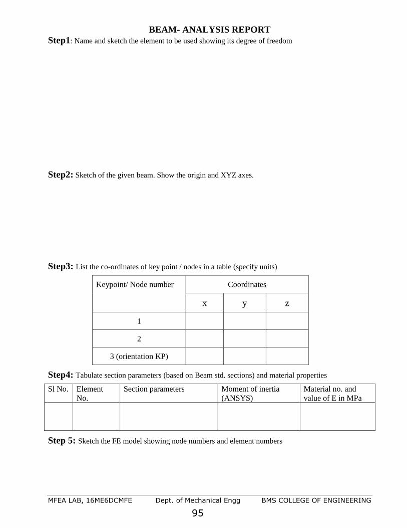
MFEA LAB, 16ME6DCMFE Dept. of Mechanical Engg BMS COLLEGE OF ENGINEERING
95
BEAM- ANALYSIS REPORT
Step1: Name and sketch the element to be used showing its degree of freedom
Step2: Sketch of the given beam. Show the origin and XYZ axes.
Step3: List the co-ordinates of key point / nodes in a table (specify units)
Keypoint/ Node number Coordinates
x y z
1
2
3 (orientation KP)
Step4: Tabulate section parameters (based on Beam std. sections) and material properties
Sl No. Element
No.
Section parameters Moment of inertia
(ANSYS)
Material no. and
value of E in MPa
Step 5: Sketch the FE model showing node numbers and element numbers

MFEA LAB, 16ME6DCMFE Dept. of Mechanical Engg BMS COLLEGE OF ENGINEERING
96
Step 6: List
a) Displacement boundary conditions to be incorporated
Node No. Ux Uy Uz Rotx Roty Rotz
Translations are in mm and rotations are in radians
b) Force/Moment boundary conditions to be incorporated
Node No. Fx Fy Fz Mx My Mz
Forces are in N and Moments are in N-mm
Solution:
Step7: List Reaction solution
Node No. Rx Ry Rz RMx RMy RMz
Show them on the sketch and check for ΣFx= 0, ΣFy=0, ΣFz=0, ΣMx= 0, ΣMy=0, ΣMz=0,
Also calculate reactions from fundamentals and compare with the ANSYS values. Ensure that they are
same, else doesn’t proceed.

MFEA LAB, 16ME6DCMFE Dept. of Mechanical Engg BMS COLLEGE OF ENGINEERING
97
Step8:
Nodal Displacements and rotations with units
Node No. Ux Uy Uz Rotx Roty Rotz
Highlight/ specify node with maximum displacements
Step9: List Shear force and Bending Moment Values with units. Specify:
ETABLE Item and sequence number for shear forces:
ETABLE Item and sequence number for Bending moment:
Element
No.
Shear Forces on Elements Bending Moment Values
I - node J - node I - node J - node

MFEA LAB, 16ME6DCMFE Dept. of Mechanical Engg BMS COLLEGE OF ENGINEERING
98
Step10: List bending stress with units.
Specify: ETABLE Item and sequence number for bending stress:
Element
No.
Top Fiber Bottom Fiber
I - node J - node I - node J - node
Highlight maximum stress with location
Step11: Conclusion
1) Critical element/ location is …………. and the stress value is………….
2) Maximum displacement point / node is ……………… and value is……………
3) Maximum shear force is …………. and occurs at ………..
4) Maximum bending moment is ……… and occurs at……………
5) Sketch the followings, one below the other (must be written in a single page):

MFEA LAB, 16ME6DCMFE Dept. of Mechanical Engg BMS COLLEGE OF ENGINEERING
99
FE model with Node no.s, Element
No.s, BCs
Applied loads & reactions
Displacement plot
Shear force diagram
Bending moment diagram

MFEA LAB, 16ME6DCMFE Dept. of Mechanical Engg BMS COLLEGE OF ENGINEERING
100
Solution from Strength of Materials:
* From SOM , calculate Theoretical Maximum, Bending stress Maximum. Also write SFD
&BMD diagram (SFD5, SFD18, BMD2, BMD15)
30. a) Effect of Self Weight on a Cantilever Beam. The beam is to be made of steel with a modulus
of elasticity of 200 GPa. L=1000mm, W=10mm, h=50mm. Density= 7860 Kg/m3.
Compare and explain the influence of moment of Inertia on deflection and stresses with that of
problem 30. Is there any change in SFD and BMD?
Sl.
No.
Particular Maximum
value with
units
Maximum value
from problem
30
remarks
1 Moment of inertia
2 Deflection
3 Stress
4 Shear force
5 Bending moment
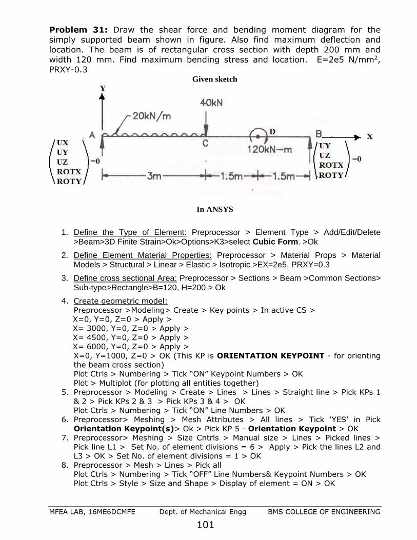
MFEA LAB, 16ME6DCMFE Dept. of Mechanical Engg BMS COLLEGE OF ENGINEERING
101
Problem 31: Draw the shear force and bending moment diagram for the simply supported beam shown in figure. Also find maximum deflection and
location. The beam is of rectangular cross section with depth 200 mm and width 120 mm. Find maximum bending stress and location. E=2e5 N/mm2,
PRXY-0.3 Given sketch
In ANSYS
1. Define the Type of Element: Preprocessor > Element Type > Add/Edit/Delete >Beam>3D Finite Strain>Ok>Options>K3>select Cubic Form. >Ok
2. Define Element Material Properties: Preprocessor > Material Props > Material Models > Structural > Linear > Elastic > Isotropic >EX=2e5, PRXY=0.3
3. Define cross sectional Area: Preprocessor > Sections > Beam >Common Sections> Sub-type>Rectangle>B=120, H=200 > Ok
4. Create geometric model:
Preprocessor >Modeling> Create > Key points > In active CS > X=0, Y=0, Z=0 > Apply > X= 3000, Y=0, Z=0 > Apply >
X= 4500, Y=0, Z=0 > Apply > X= 6000, Y=0, Z=0 > Apply >
X=0, Y=1000, Z=0 > OK (This KP is ORIENTATION KEYPOINT - for orienting the beam cross section)
Plot Ctrls > Numbering > Tick “ON” Keypoint Numbers > OK
Plot > Multiplot (for plotting all entities together) 5. Preprocessor > Modeling > Create > Lines > Lines > Straight line > Pick KPs 1
& 2 > Pick KPs 2 & 3 > Pick KPs 3 & 4 > OK Plot Ctrls > Numbering > Tick “ON” Line Numbers > OK
6. Preprocessor> Meshing > Mesh Attributes > All lines > Tick ‘YES’ in Pick
Orientation Keypoint(s)> Ok > Pick KP 5 - Orientation Keypoint > OK 7. Preprocessor> Meshing > Size Cntrls > Manual size > Lines > Picked lines >
Pick line L1 > Set No. of element divisions = 6 > Apply > Pick the lines L2 and L3 > OK > Set No. of element divisions = 1 > OK
8. Preprocessor > Mesh > Lines > Pick all
Plot Ctrls > Numbering > Tick “OFF” Line Numbers& Keypoint Numbers > OK Plot Ctrls > Style > Size and Shape > Display of element = ON > OK

MFEA LAB, 16ME6DCMFE Dept. of Mechanical Engg BMS COLLEGE OF ENGINEERING
102
Solution Phase: Assigning Loads and Solving
9. Preprocessor > Loads > Define Loads > apply > Structural
Displacement > On Nodes > Pick staring node > Ok >Select UX,UY,UZ, ROTX,ROTY > Ok
10. Preprocessor > Loads > Define Loads > apply > Structural Displacement > On Nodes > Pick the last node > Ok >Select UY,UZ
ROTX,ROTY > Ok 11. Preprocessor >loads > Define Loads > apply > Structural >
Force/Moment > On Nodes > Pick Node no.2 > Ok > Select FY= -40000> OK
12. Preprocessor >loads > Define Loads > apply > Structural > Force/Moment > On Nodes > Pick Node no.14 > Ok > Select MZ= -
120e6> OK 13. Preprocessor >loads > Define Loads > apply > Structural >
Pressure > On beams >Click Box option>Drag a window selecting
elements first 6 elements > Ok >LKEY=1, VALI=20> OK 14. Solution>Solve>Current LS>SOLVE> ‘Solution is Done’ > Close 15. General Post Processor > List Results > Nodal Solutions> DOF
Solution>Displacement vector sum>OK > You will get a list as shown below:
16. General Post Processor > List Results > Nodal Solutions> DOF Solution>Rotation
vector sum>OK >
* The above values are in radians

MFEA LAB, 16ME6DCMFE Dept. of Mechanical Engg BMS COLLEGE OF ENGINEERING
103
17. General Post Processor > Plot Results >Deformed Shape > Select Def + Undeformed > OK (Blue line indicates deformed shape and white line indicates
original shape Carry out animation also: Plot Ctrls > Animate > Deformed Shape >
Def+undeformed > Ok
18. General Post Processor > List Results > Reaction Solutions> all items >OK >
note down the values. Check for equilibrium
REACTION SOLUTIONS in Newton
19. General post processor > Element table > Define table > Add > set user
label for item = SFD5, select item, comp, results data item = by sequence number- select SMISC, 5 (Type 5 after selecting SMISC) >
Apply > set user label for item = SFD18, select item, comp, results data item = by sequence number- select SMISC, 18 (Type 18 after selecting
SMISC) > Apply > set user label for item = BMD2, select item, comp,
results data item = by sequence number- select SMISC,2 (Type 2 after selecting SMISC) > Apply > set user label for item = BMD15, select
item, comp, results data item = by sequence number- select SMISC, 15 (Type 15 after selecting SMISC) > Apply > OK > Close
20. General Post Processor > Element Table > List Element Table > Select SFD5, SFD18, BMD2, BMD15 > OK > Note the
shear Forces and Note the Bending Moments
21. General Post Processor >Plot Results > contour plot > Line element res> Select SFD5, SFD18, > OK > SFD will be displayed
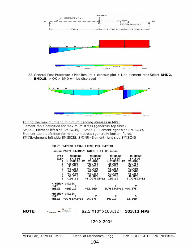
MFEA LAB, 16ME6DCMFE Dept. of Mechanical Engg BMS COLLEGE OF ENGINEERING
104
22. General Post Processor >Plot Results > contour plot > Line element res>Select BMD2,
BMD15, > OK > BMD will be displayed
To find the maximum and minimum bending stresses in MPa:
Element table definition for maximum stress (generally top fibre)
SMAXL -Element left side SMISC34, SMAXR - Element right side SMISC39,
Element table definition for minimum stress (generally bottom fibre),
SMINL-element left side SMISC35, SMINR -Element right side SMISC40
NOTE: = 82.5 X106 X100x12 = 103.13 MPa
120 X 2003

MFEA LAB, 16ME6DCMFE Dept. of Mechanical Engg BMS COLLEGE OF ENGINEERING
105
SOM solution for Problem 31
Draw the shear force and bending moment diagram for the beam shown in figure. Also find
maximum deflection and location. The beam is of rectangular cross section with depth 200 mm and
width 120 mm. Find maximum bending stress and location.

MFEA LAB, 16ME6DCMFE Dept. of Mechanical Engg BMS COLLEGE OF ENGINEERING
106
Problem32: Draw the shear force and bending moment diagram for the following problem.
Also determine displacement field, Maximum bending stress, and reactions by taking it as a
Rectangular c/s with depth 20 mm and thickness 10mm. Take v= 0.3, E= 2x10⁵N/mm2.
1”
SFD5, SFD18, BMD2, BMD15
Results:
ELEMENTAL SOLUTION- Shear Force and Bending Moment(Mention the units also)
Results: ELEMENTAL SOLUTION-Bending Stresses
Max stress:____________ Location:____________
Max deflection:________________ Location:____________
Slope at tip:
Element
No.
Shear Forces on Elements Bending Moment Values
SFD5 SFD18 BMD2 BMD15
1
2
3
4
Element
No.
Bending Stresses SMAXL34 SMAXR39 SMINL 35 SMINR 40
1
2
3
4
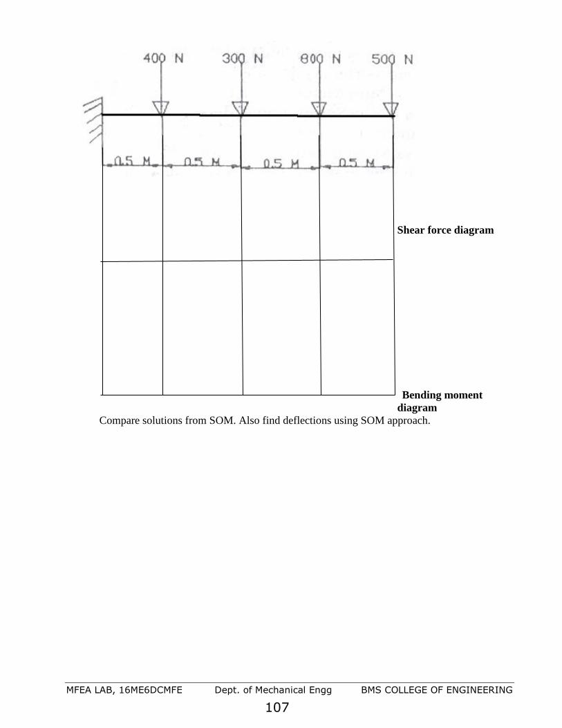
MFEA LAB, 16ME6DCMFE Dept. of Mechanical Engg BMS COLLEGE OF ENGINEERING
107
Shear force diagram
Bending moment
diagram
Compare solutions from SOM. Also find deflections using SOM approach.

MFEA LAB, 16ME6DCMFE Dept. of Mechanical Engg BMS COLLEGE OF ENGINEERING
108
Problem33: Find the shear force and bending moments and draw diagrams for the following problem. Data: Rectangular c/s depth 120 mm, thickness 10mm, v= 0.3, E= 2x10⁵N/mm2 Also determine displacement field, Maximum bending stress, and reactions.
SOLUTION:
Shear force diagram
Bending moment diagram
Results: ELEMENTAL SOLUTION- Shear Force and Bending Moment:
Element No.
Shear Forces on Elements Bending Moment Values
SFD5 SFD18 BMD2 BMD15
1
2
3
4
5
6
7
8
9
10
11
12

MFEA LAB, 16ME6DCMFE Dept. of Mechanical Engg BMS COLLEGE OF ENGINEERING
109
Results: ELEMENTAL SOLUTION- Bending stresses
Also obtain maximum stress, maximum deflection and locations
Problem 34: A long cantilever beam with 30 mm square cross-section and 1000 mm length (see figure below) is subjected to (a) Concentrated tip force (b) Concentrated tip moment (c) Distributed pressure load Each loading is applied separately.
Loading Deflection (mm) Bending Moment (N-mm)
Max. Bending Stress (N/mm2)
ANSYS Theory ANSYS Theory ANSYS Theory
Case A F=10KN
Case B M=10KN-m
Case C P=5MPa
Element No. Bending stresses
SMAXL34 SMAXR39 SMINL 35 SMINR 40
1
2
3
4
5
6
7
8
9
10
11
12

MFEA LAB, 16ME6DCMFE Dept. of Mechanical Engg BMS COLLEGE OF ENGINEERING
110
Problem 35:A long cantilever beam with 30 mm square cross-section and 1000 mm
length is subjected to an off-centered axial force of 1000 N (see figure below). The force is offset by 100 mm. E=70GPa
Result Node No.
Deflection (mm)
Node No. Bending Moment (N-mm)
Element No.
Max. Bending Stress (N/mm2)
ANSYS Analysis
Theory
Problem 36: Determine the end forces of a clamped-clamped beam due to a 25 mm settlement at the right end. Take 10 Elements A = 50 X 50 Sq. E = 200 Gpa L = 2 m
A= 50X50 sq
25
Reactions:
Fx=1000N
Mz=1000 X 100N-mm
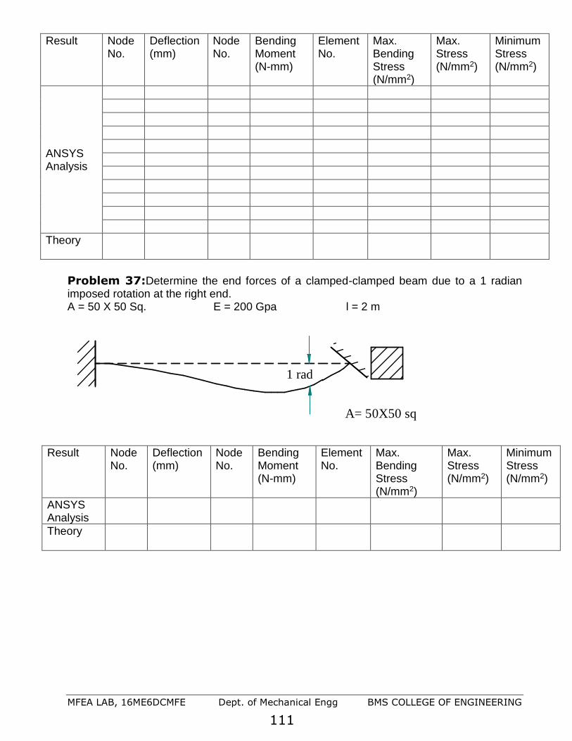
MFEA LAB, 16ME6DCMFE Dept. of Mechanical Engg BMS COLLEGE OF ENGINEERING
111
Result Node No.
Deflection (mm)
Node No.
Bending Moment (N-mm)
Element No.
Max. Bending Stress (N/mm2)
Max. Stress (N/mm2)
Minimum Stress (N/mm2)
ANSYS Analysis
Theory
Problem 37:Determine the end forces of a clamped-clamped beam due to a 1 radian imposed rotation at the right end. A = 50 X 50 Sq. E = 200 Gpa l = 2 m
A= 50X50 sq
1 rad
Result Node No.
Deflection (mm)
Node No.
Bending Moment (N-mm)
Element No.
Max. Bending Stress (N/mm2)
Max. Stress (N/mm2)
Minimum Stress (N/mm2)
ANSYS Analysis
Theory

MFEA LAB, 16ME6DCMFE Dept. of Mechanical Engg BMS COLLEGE OF ENGINEERING
112
Problem 38: A beam of length L and height h is built-in at one end and loaded at free end with (A) a shear force F, and (B) a moment M. Determine the deflection at the free end. A = 50 X 50 Sq. E = 200 Gpa L = 2 m
Result Node
No. Deflection (mm)
Node No.
Bending Moment (N-mm)
Element No.
Max. Bending Stress (N/mm2)
Max. Stress (N/mm2)
Minimum Stress (N/mm2)
ANSYS Analysis
Theory
Problem 39: The figure shows a loaded beam subjected to various types of loading E =
200 GPa , I = 4 X 106 mm4
Result Max Deflection (mm)
Node No. Bending Moment (N-mm)
Element No.
Max. Bending location Stress (N/mm2)
ANSYS Analysis
Theory
Hint: Assume it as a square cross section; calculate the dimension from the given value of moment of inertia

MFEA LAB, 16ME6DCMFE Dept. of Mechanical Engg BMS COLLEGE OF ENGINEERING
113
Problem 40: A long cantilever beam has an I cross section with a total depth of
150mm , flange width of 100mm , thickness of flange and web being 25mm. Length of the beam is 1000 mm (see figure below) and is subjected to (a) Concentrated tip force (b) Concentrated tip moment (c) Distributed pressure load. Each loading is applied separately
A=
Loading Deflection (mm) Bending Moment (N-mm)
Max. Bending Stress (N/mm2)
ANSYS Theory ANSYS Theory ANSYS Theory
Case A F=10KN
Case B M=10KN-m
Case C P=5MPa

MFEA LAB, 16ME6DCMFE Dept. of Mechanical Engg BMS COLLEGE OF ENGINEERING
114
Problem 41: Draw the shear force and bending moment diagram for the beam shown in figure. Also find maximum deflection and location .The beam is of rectangular cross section with depth 300 mm and width 200 mm. Find maximum stress and location. .E =200GPa.
Results: ELEMENTAL SOLUTION- Shear Force and Bending Moment,and Axial thrust
Results: ELEMENTAL SOLUTION- stresses
Also obtain maximum stress, maximum deflection and their locations
Element
No.
Shear Forces on Elements
Bending Moment
Values Axial thrust
SFD5 SFD18 BMD2 BMD15 Mforx1(SMISC,1) Mforx7(SMISC,14)
1
2
3
4
Element
No. stresses
SMAXL SMAXR SMINL SMINR
1
2
3
4

MFEA LAB, 16ME6DCMFE Dept. of Mechanical Engg BMS COLLEGE OF ENGINEERING
115
Problem 42: Draw the shear force and bending moment diagram for the beam shown in figure. Also find maximum deflection and location. Cross section is I with a total depth of 150mm, flange width of 100mm, thickness of flange and web being 25mm. Find maximum stress and location. .E =200GPa.
80KN
3000 1500 1500
500
40 KN/m
Results: ELEMENTAL SOLUTION- Shear Force and Bending Moment:
Results: ELEMENTAL SOLUTION- Bending stresses
Also obtain maximum stress, maximum deflection and their locations
Element
No.
Shear Forces on Elements Bending Moment Values
SFD5 SFD18 BMD2 BMD15
1
2
3
4
5
6
7
8
9
10
11
12
Element
No.
Bending stresses
SMAXL SMAXR SMINL SMINR
1
2
3
4
5
6
7
8
9
10
11
12

MFEA LAB, 16ME6DCMFE Dept. of Mechanical Engg BMS COLLEGE OF ENGINEERING
116
Problems on TORSION of shafts
Problem 43: A Stepped shaft is subjected to torque as shown in fig. Determine the angle
of twist at the free end and twist in each portion in degrees. Also find the maximum shear stress in each step. Young’s modulus=208GPa, poisons ratio=0.3 Case a) Procedure for BEAM model:
Tabulate the node-coordinate data. 1. Preferences > structural > Ok 2. Preprocessor > ELEMENT type > Add/edit/delete > add > Beam- 3D finite strain > OK > CLOSE 3. Preprocessor > Material Props >Material Model >Structural > Elastic>Isotropic> EX=208GPa, PRXY=0.3>OK 4. Preprocessor > Section > Beam >Common Sections.
On the beam Tool dialog box, enter ’1’ for ID, ‘Section1” for Name, Choose Hollow Cross-Section for Sub-Type, enter Ri=40, Ro=50 Apply. 5. On the beam Tool dialog box, enter ’2’ for ID, ‘Section2” for Name, Choose Circular Solid Cross-Section for Sub-Type, Enter R=40, Apply . 6. On the beam Tool dialog box, enter ’3’ for ID, ‘Section3” for Name, Choose Circular Solid Cross-Section for Sub-Type, enter R=30, ok. 7. Preprocessor >Modeling> Create > Nodes > In active CS >
Node No:=1, X=0, Y=0, Z=0 > Apply Node No:=2, X=300, Y=0, Z=0 > Apply Node No:=3, X=700, Y=0, Z=0 > Apply Node No:=4, X=1200,Y=0, Z=0 > OK
8. Preprocessor > Modeling > Create > elements >Element Attributes> Section number>Section1>OK 9. Preprocessor > Modeling > Create > elements Thru Nodes > 1 & 2 nodes > OK 10. Preprocessor > Modeling > Create > elements >Element Attributes>Section number> Section2>OK 11. Preprocessor > Modeling > Create > elements Thru Nodes > Pick 2 & 3 nodes > OK
Node No Coordinate
X (mm) Y (mm) Z (mm)
1 0 0 0
2 300 0 0
3 700 0 0
4 1200 0 0

MFEA LAB, 16ME6DCMFE Dept. of Mechanical Engg BMS COLLEGE OF ENGINEERING
117
12. Preprocessor > Modeling > Create > elements >Element Attributes>Section number>Section3>OK 13. Preprocessor > Modeling > Create > elements Thru Nodes > Pick 3 & 4 nodes > OK 14. Utility Menu > PlotCtrls>Style>Size and Shape > On Size and Shape dialog box turn ON [/ESHAPE] display of Element and click OK. 15. In the Utility Menu, select Plot> Elements. 16. Switch to isometric view using the pan-Zoom-Rotate dialog box. 17. Preprocessor>Loads>DefineLoads>Apply>Structural> Displacement> On Nodes>select Node1>OK>ALLDOF>OK 18. Preprocessor>Loads>DefineLoads>Apply>Structural> Force/Moment> On Nodes>select Node2>OK>Direction of force/mom=MX, Value= 3e6>Apply 19. Preprocessor>Loads>DefineLoads>Apply>Structural>Force/Moment > On Nodes>select Node3>OK>Direction of force/mom=MX, Value= -2e6>Apply 20. Preprocessor>Loads>DefineLoads>Apply>Structural>Force/Moment >On Nodes>select Node4>OK>Direction of force/mom=MX, Value= 1e6>OK 21. Solution>Solve>Current LS>OK, Close Solution Done Window. RESULTS: Nodal solution: 22. General Postproc>Plot result>Contour Plot>NodalSolu. On the Contour Nodal Solution Data dialog box, Nodal solution>DOF Solution> Select Rotation vector sum>OK 23. General postprocessor>List Results>Nodal Solutions>OK>DOF Solution>Rotation vector sum>OK (in radians)
Reaction solution: 24. General Postproc>List results>Reaction Solution>All Items>OK
Element Solution:
25. General post processor > Element table > Define table > Add > set user label for item = TQ4, select item, comp, results data item = by sequence
number- select SMISC, 4 (Type 4 after selecting SMISC) > Apply > set user label for item = TQ17, select item, comp, results data item = by sequence

MFEA LAB, 16ME6DCMFE Dept. of Mechanical Engg BMS COLLEGE OF ENGINEERING
118
number- select SMISC, 17 (Type 17 after selecting SMISC) > Apply > OK > Close
26. General Post Processor > Element Table > List Element Table > Select TQ4, TQ17>OK > Note the Torsional Moments in N-mm
27. General Post Processor > Plot results >Contour plot> Element Table >
Select TQ4, TQ17>OK NOTE: We can only find torsional moments as we are using BEAM element. We can get shear stresses in each portion by using PIPE288 element Case b) Procedure for PIPE model: 1. Preferences > structural > Ok 2. Preprocessor > ELEMENT type > Add/edit/delete > add > Pipe- 3D finite strain > OK > Options > Hoop strain treatment = Thick shell > OK > CLOSE 3. Preprocessor > Material Props >Material Model >Structural > Elastic>Isotropic> EX=208GPa, PRXY=0.3>OK 4. Preprocessor > Section > Pipe >Add > Add pipe section with ID = 1, ok > Section name = Section1, Pipe diameter = 100, Wall thickness = 10, Apply > Add pipe section with ID = 2, ok > Section name = Section2, Pipe diameter = 80, Wall thickness = 40, Apply > Add pipe section with ID = 3, ok > Section name = Section3, Pipe diameter = 60, Wall thickness = 30, Ok (Close the warning message) 5. Preprocessor >Modeling> Create > Nodes > In active CS >
Node No:=1, X=0, Y=0, Z=0 > Apply Node No:=2, X=300, Y=0, Z=0 > Apply Node No:=3, X=700, Y=0, Z=0 > Apply Node No:=4, X=1200,Y=0, Z=0 > OK
6. Preprocessor > Modeling > Create > elements >Element Attributes> Section number>Section1>OK 7. Preprocessor > Modeling > Create > elements Thru Nodes > 1 & 2 nodes > OK 8. Preprocessor > Modeling > Create > elements >Element Attributes>Section number> Section2>OK 9. Preprocessor > Modeling > Create > elements Thru Nodes > Pick 2 & 3 nodes > OK 10. Preprocessor > Modeling > Create > elements >Element Attributes>Section number>Section3>OK 11. Preprocessor > Modeling > Create > elements Thru Nodes > Pick 3 & 4 nodes > OK 12. Utility Menu > PlotCtrls>Style>Size and Shape > On Size and Shape dialog box turn ON [/ESHAPE] display of Element and click OK. 13. In the Utility Menu, select Plot> Elements. 14. Switch to isometric view using the pan-Zoom-Rotate dialog box.
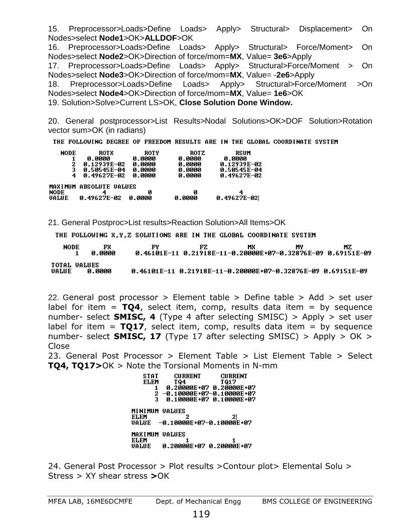
MFEA LAB, 16ME6DCMFE Dept. of Mechanical Engg BMS COLLEGE OF ENGINEERING
119
15. Preprocessor>Loads>Define Loads> Apply> Structural> Displacement> On Nodes>select Node1>OK>ALLDOF>OK 16. Preprocessor>Loads>Define Loads> Apply> Structural> Force/Moment> On Nodes>select Node2>OK>Direction of force/mom=MX, Value= 3e6>Apply 17. Preprocessor>Loads>Define Loads> Apply> Structural>Force/Moment > On Nodes>select Node3>OK>Direction of force/mom=MX, Value= -2e6>Apply 18. Preprocessor>Loads>Define Loads> Apply> Structural>Force/Moment >On Nodes>select Node4>OK>Direction of force/mom=MX, Value= 1e6>OK 19. Solution>Solve>Current LS>OK, Close Solution Done Window. 20. General postprocessor>List Results>Nodal Solutions>OK>DOF Solution>Rotation vector sum>OK (in radians)
21. General Postproc>List results>Reaction Solution>All Items>OK
22. General post processor > Element table > Define table > Add > set user label for item = TQ4, select item, comp, results data item = by sequence
number- select SMISC, 4 (Type 4 after selecting SMISC) > Apply > set user label for item = TQ17, select item, comp, results data item = by sequence
number- select SMISC, 17 (Type 17 after selecting SMISC) > Apply > OK > Close
23. General Post Processor > Element Table > List Element Table > Select
TQ4, TQ17>OK > Note the Torsional Moments in N-mm
24. General Post Processor > Plot results >Contour plot> Elemental Solu > Stress > XY shear stress >OK

MFEA LAB, 16ME6DCMFE Dept. of Mechanical Engg BMS COLLEGE OF ENGINEERING
120
Check with SOM solution:

MFEA LAB, 16ME6DCMFE Dept. of Mechanical Engg BMS COLLEGE OF ENGINEERING
121
PART-B
Chapter 08: 2D Analysis
Plate Problems
Examples: Thin Plate with a hole subjected to in plane loading, rotating disk or flywheel
Examples:wall of a dam, Strip footing, rotating shaft or cylinder

MFEA LAB, 16ME6DCMFE Dept. of Mechanical Engg BMS COLLEGE OF ENGINEERING
122
Plate with a hole: Can be solved as Bi-axial symmetry problem, as shown below
PLANE182 Element Description: 2-D 4-Node Structural Solid

MFEA LAB, 16ME6DCMFE Dept. of Mechanical Engg BMS COLLEGE OF ENGINEERING
123
PLANE182 is used for 2-D modeling of solid structures. The element can be used as either
a plane element (plane stress, plane strain or generalized plane strain) or an axisymmetric
element. It is defined by four nodes having two degrees of freedom at each node:
translations in the nodal x and y directions. The element has plasticity, hyperelasticity,
stress stiffening, large deflection, and large strain capabilities. It also has mixed formulation
capability for simulating deformations of nearly incompressible elastoplastic materials, and
fully incompressible hyperelastic materials.
PLANE182 Geometry
PLATE PROBLEMS

MFEA LAB, 16ME6DCMFE Dept. of Mechanical Engg BMS COLLEGE OF ENGINEERING
124
Meshing – An important step:
Free meshing v/s Mapped Meshing:

MFEA LAB, 16ME6DCMFE Dept. of Mechanical Engg BMS COLLEGE OF ENGINEERING
125
Problem 44. Obtain Stress concretion factor for a Plate with hole under tension, Young’s modulus=200GPa, PRXY=0.3
Preprocessing: Defining the Problem:-
Step-1 Preprocessor Menu > Element Type > Add/Edit/Delete > add Solid and Quad 4node
182>Ok> Option>K3-Plane strs w/thk>Ok>Close
Step 2 Preprocessor > Real Constants > Add/Edit/Delete >Add>Ok>thk 20>Ok>Close
Step 3 Preprocessor > Material Props > Material models > Structural > Linear > Elastic >
Isotropic > EX20e4, PRXY 0.3>OK> Close
Step 4 Preprocessor > Modeling > Create > Areas > Rectangle > By 2 Corners>X0,Y0 Width
100 and Height 50>OK
Step 5 Preprocessor > Modeling > Create > Areas > Circle > Solid Circle > X0, Y0, R20 >Ok
Step 6 Preprocessor > Modeling > Operate > Booleans > Subtract > Areas
Therefore, select the base area (the rectangle) by clicking on it. Note: The selected area will turn
pink once it is selected. The following window may appear because there are 2 areas at the location
you clicked.
Ensure that the entire rectangular area is selected (otherwise click 'Next') and then click 'OK'. Click
'OK' on the 'Subtract Areas' window. Now you will be prompted to select the areas to be subtracted,
select the circle by clicking on it and then click 'OK'.
Here w=100 mm, a=40mm, t=20mm

MFEA LAB, 16ME6DCMFE Dept. of Mechanical Engg BMS COLLEGE OF ENGINEERING
126
Step 7 Preprocessor > Meshing > Size Cntrls > Manual Size > Areas > All Areas > 25>OK
NOTE: Deciding the mesh size/element size is based on the geometry, level of accuracy required and
type of element used. Here, element size must be such that mesh includes at least 2 elements at the
arc of the hole. Later, this number is increased to improve the accuracy of the solution (convergence
study).
Step 8 Meshing > Mesh > Areas > Free> Pick the rectangle>Ok> li
Note down the total number of elements and nodes
Solution Phase: Assigning Loads and Solving:-
Step 09 Define Analysis Type :Solution > Analysis Type > New Analysis>Static> OK
Step 10 Apply Constraints :Solution > Define Loads > Apply > Structural > Displacement >
Symmetric B.C> on Lines> Select Left side and bottom> OK
Step 11 Apply Loads :Solution > Define Loads > Apply > Structural > Pressure > On Lines>
Select the Right end of the plate and click on 'Apply’>Load PRES value = (-1) > OK
Note: a) Calculate the pressure on the plate end by dividing the distributed load by the
thickness of the plate (1 MPa).
b) The pressure is uniform along the surface of the plate, therefore the last field is left
blank.
c) The pressure is acting away from the surface of the plate, and is therefore defined as
a negative pressure
Step 12 Solving the System : Solution > Solve > Current LS> Ok
Postprocessing: Viewing the Results
Step 13 ANSYS : Utility Menu > Plot > Nodes>Utility Menu > PlotCtrls > Numbering
(The plot should look similar to the one shown below. Make a note of the node closest to the top of
the circle (ie. #25)

MFEA LAB, 16ME6DCMFE Dept. of Mechanical Engg BMS COLLEGE OF ENGINEERING
127
Step 14 Postproc > List Results > Nodal Solution > Stress, von Mises stress>Ok
The Von Mises Stress was found to be 2.5494 MPa at this point. We will use smaller elements to try
to get a more accurate solution.
Step 15 Deformation: Genrl Postproc > Plot Results >Deformed Shape >Def + undeformd >Ok
Step16 Deflection : General Postproc > Plot Results > Contour plot>Nodal Solution> DOF >
Solution> Displacement vector sum>OK

MFEA LAB, 16ME6DCMFE Dept. of Mechanical Engg BMS COLLEGE OF ENGINEERING
128
Step17 Stresses: General Postproc > Plot Results > Nodal Solution> Stress> von Misesstress.
Contour Plot of Mises Equivalent
The Mises equivalent stress, stress_bar, is given by the equation :
In applying the Von Mises yield criterion, yielding is predicted to occur when σmises_eq=σy where σy
is the yield stress measured under uniaxial tension.
Viewing results for the Mises Equivalent Stress can provide insight into the load causing initial
yielding and the initial shape of yielding zones.
MAIN MENU -> General Postproc -> Plot Results-> Contour Plot-nodal solu...
COUNTOUR NODAL SOLUTION DATA -> Highlight Stress
COUNTOUR NODAL SOLUTION DATA -> Highlight von Mises SEQV
COUNTOUR NODAL SOLUTION DATA -> OK
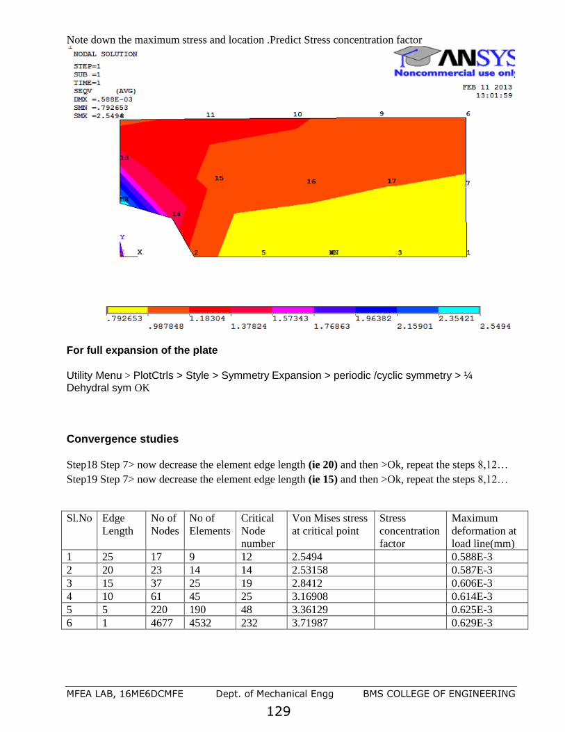
MFEA LAB, 16ME6DCMFE Dept. of Mechanical Engg BMS COLLEGE OF ENGINEERING
129
Note down the maximum stress and location .Predict Stress concentration factor
For full expansion of the plate
Utility Menu > PlotCtrls > Style > Symmetry Expansion > periodic /cyclic symmetry > ¼ Dehydral sym OK
Convergence studies
Step18 Step 7> now decrease the element edge length (ie 20) and then >Ok, repeat the steps 8,12…
Step19 Step 7> now decrease the element edge length (ie 15) and then >Ok, repeat the steps 8,12…
Sl.No Edge
Length
No of
Nodes
No of
Elements
Critical
Node
number
Von Mises stress
at critical point
Stress
concentration
factor
Maximum
deformation at
load line(mm)
1 25 17 9 12 2.5494 0.588E-3
2 20 23 14 14 2.53158 0.587E-3
3 15 37 25 19 2.8412 0.606E-3
4 10 61 45 25 3.16908 0.614E-3
5 5 220 190 48 3.36129 0.625E-3
6 1 4677 4532 232 3.71987 0.629E-3

MFEA LAB, 16ME6DCMFE Dept. of Mechanical Engg BMS COLLEGE OF ENGINEERING
130
As the number of elements in the mesh increases (i.e. the element edge length decreases), the values
converge towards a final solution.
Graph Stresses in Cross Section
• MAIN MENU -> General Postproc -> Path Operations -> Define Path-By Nodes
• DEFINE PATH -> Pick nodes along the left edge of the plate towards the hole. Click OK.
• In the Define Path Name box, type: 1, click OK.
• PATH OPERATIONS -> Map Onto Path, MAP RESULTS ITEMS ONTO PATH -> Highlight
Stress, MAP RESULTS ITEMS ONTO PATH -> Highlight X-Direction SX or whichever stress
component is relevant.
• MAP RESULTS ITEMS ONTO PATH -> OK
• PATH OPERATIONS -> Plot Path Items -On Graph
• PATH PLOT OF PATH ITEMS -> Highlight SX
• PATH PLOT OF PATH ITEMS -> OK
Calculated net stress concentration factor (SCF):
Load, F=P x w x t =
nominal=F/[(w-a)t] =
K=max/nominal=
max= Maximum value of Sxx on hole boundary at =900=
Compare this value with that obtained from Data Hand Book.
The von Mises stress at the top of the hole in the plate was found to be approximately 3.8 MPa. This
is a mere 2.5% difference between the analytical solution and the solution found using ANSYS.
Note: Refer appendix on the page No 233
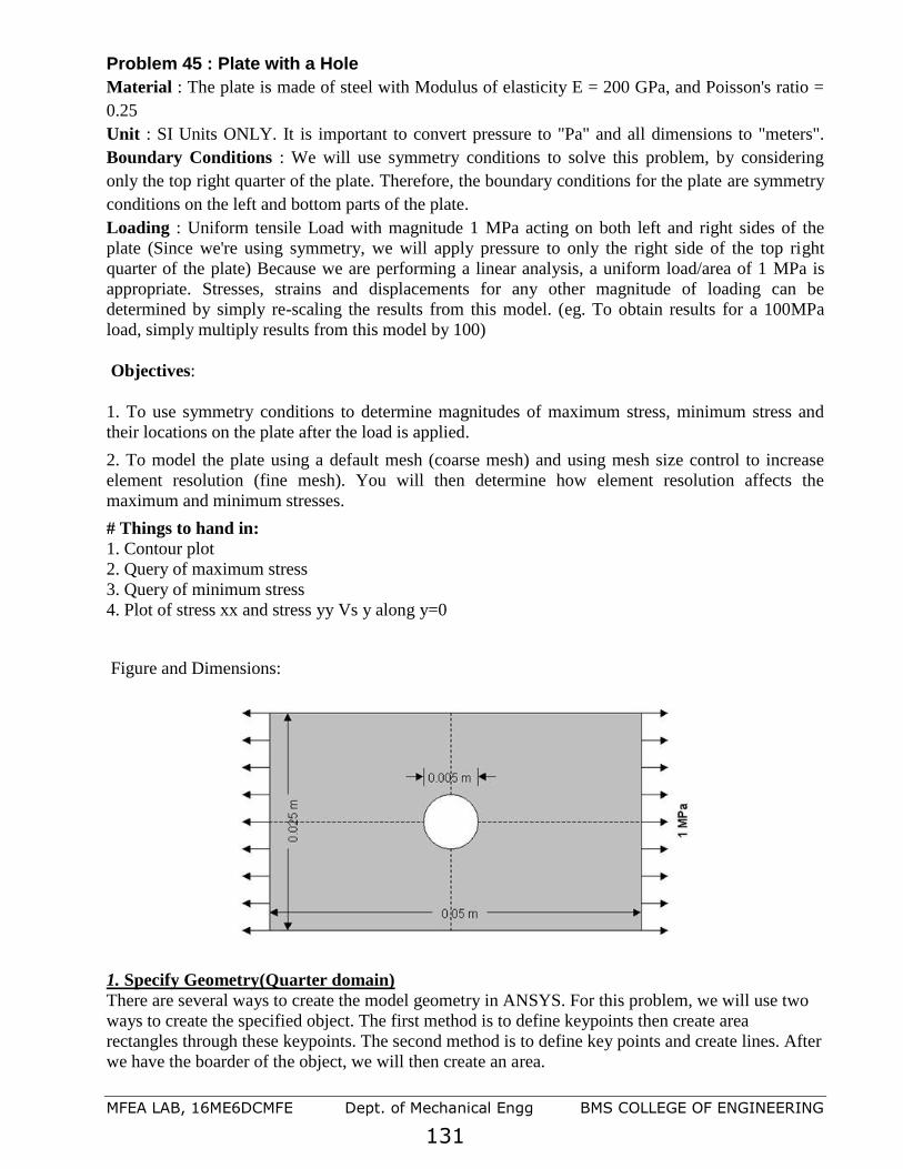
MFEA LAB, 16ME6DCMFE Dept. of Mechanical Engg BMS COLLEGE OF ENGINEERING
131
Problem 45 : Plate with a Hole
Material : The plate is made of steel with Modulus of elasticity E = 200 GPa, and Poisson's ratio =
0.25
Unit : SI Units ONLY. It is important to convert pressure to "Pa" and all dimensions to "meters".
Boundary Conditions : We will use symmetry conditions to solve this problem, by considering
only the top right quarter of the plate. Therefore, the boundary conditions for the plate are symmetry
conditions on the left and bottom parts of the plate.
Loading : Uniform tensile Load with magnitude 1 MPa acting on both left and right sides of the
plate (Since we're using symmetry, we will apply pressure to only the right side of the top right
quarter of the plate) Because we are performing a linear analysis, a uniform load/area of 1 MPa is
appropriate. Stresses, strains and displacements for any other magnitude of loading can be
determined by simply re-scaling the results from this model. (eg. To obtain results for a 100MPa
load, simply multiply results from this model by 100)
Objectives:
1. To use symmetry conditions to determine magnitudes of maximum stress, minimum stress and
their locations on the plate after the load is applied.
2. To model the plate using a default mesh (coarse mesh) and using mesh size control to increase
element resolution (fine mesh). You will then determine how element resolution affects the
maximum and minimum stresses.
# Things to hand in:
1. Contour plot
2. Query of maximum stress
3. Query of minimum stress
4. Plot of stress xx and stress yy Vs y along y=0
Figure and Dimensions:
1. Specify Geometry(Quarter domain)
There are several ways to create the model geometry in ANSYS. For this problem, we will use two
ways to create the specified object. The first method is to define keypoints then create area
rectangles through these keypoints. The second method is to define key points and create lines. After
we have the boarder of the object, we will then create an area.

MFEA LAB, 16ME6DCMFE Dept. of Mechanical Engg BMS COLLEGE OF ENGINEERING
132
However, in order to see their numbers when creating keypoints, we will need to turn on the
keypoint numbers.
ANSYS UTILITY MENU -> PlotCtrls -> Numbering>on
check the box next to "Keypoint numbers" to turn it on. Then click OK to close the dialog box.
The First Method: Merging Areas
1.1 CREATE KEYPOINTS
In this step, we will create 6 keypoints needed to create the plate areas.
PREPROCESSOR -> -Modeling – Create -> -Keypoints -> In Active CS...
The input box "Create Keypoints in Active Coordinate System" should appear on the screen
Then create 6 keypoints at 6 different locations by enter the Keypoint numbers and locations as
following:
Keypoint number 1 : (0, 0, 0) -> Click Apply
Keypoint number 2 : (0.0125, 0, 0) -> Click Apply
Keypoint number 3 : (0.025, 0, 0) -> Click Apply
Keypoint number 4 : (0.025, 0.0125, 0) -> Click Apply
Keypoint number 5 : (0.0125, 0.0125, 0) -> Click Apply
Keypoint number 6 : (0, 0.0125, 0) -> Click OK
1.2 CREATE AREA THROUGH KEYPOINTS
The next step, we will create three areas through the keypoints we have created. These three areas
are arranged to allow improvements in element resolution which will also improve the accuracy of
the analysis.
PREPROCESSOR -> -Modeling – Create -> -Area –Arbitrary -> Through KPs
The Create Area Thru KPs window pops up. Pick Keypoints to create areas as followings:
1. Pick Keypoint numbers 1, 5, 6 (Pick in that order). Then click OK.
2. Pick Keypoint numbers 1, 5, 2. Click OK.
3. Pick Keypoint numbers 2, 3, 4, 5. Click OK.
Then you would have the connected area of a rectangle with three different areas in it.
1.3 CREATE CIRCULAR AREA (HOLE)
PREPROCESSOR -> -Modeling – Create -> -Area –Circle -> Partial Annulus.The Part Annular
Circ Area window should now appear on the screen. Fill in the fields Enter
WP X = 0 Circle center X-Coordinate
WP Y = 0 Circle center Y-Coordinate
Rad-1 =0 Inner radii of the circle or cylinder. A value of zero or blank, or the same value for
both Rad-1 and Rad-2, defines a solid circle or cylinder.
Theta-1 = 0 Starting angles of the circle or faces of the cylinder.
Rad-2 =0.0025 Outer radii of the circle or cylinder.
Theta-2 =90 Ending angles of the circle or faces of the cylinder.
Click OK.
1.4 SUBTRACT THE HOLE FROM PLATE
PREPROCESSOR -> -Modeling – Operate -> -Booleans –Subtract -> Areas. Pick the base areas
from which you want to subtract first (The two triangular areas) First, click on one triangle. Do not

MFEA LAB, 16ME6DCMFE Dept. of Mechanical Engg BMS COLLEGE OF ENGINEERING
133
click OK yet. Then click on another triangle. Now click OK. ANSYS will know that the two area is
the base area where the next input area will be subtracted from. Now pick the area to be subtracted
(Circular area) Click OK. You should now have a plate with a hole as shown :
1.5 MERGE GEOMETRY
To connect all parts together, we will have to merge the keypoints.
PREPROCESSOR -> Numbering Controls -> Merge Items... Choose Keypoints in the label pick
list. Then click OK to merge keypoints and close the dialog box.
Second Method: Creating Area through Key Points
1.1 Create Key Points
PREPROCESSOR-> -Modeling – Create > -Keypoints -> In Active CS...Then, pick the following
8 points:
Keypoint number 1 : (0, 0, 0) -> Click Apply
Keypoint number 2 : (0.0025,0,0) ->Clicl Apply
Keypoint number 3(0.0125, 0, 0) -> Click Apply
Keypoint number 4 : (0.025, 0, 0) -> Click Apply
Keypoint number 5 : (0.025, 0.0125, 0) -> Click Apply
Keypoint number 6 : (0.0125, 0.0125, 0) -> Click Apply
Keypoint number 7 : (0, 0.0125, 0) -> Click Apply
Keypoint number 8 : (0, 0.0025, 0) -> Click OK
Then, you will see the figure which indicates every key points created with its label.
1.2 Create Lines--Straight Lines and Arc.
Here, we have to create straight lines as well as an arc so that we get the same area as from the
previous method.
PREPROCESSOR -> Modeling -> Create -> Lines -> Lines -> Straight Lines
Then, select every line that composes the circumference of the specified object. Now, we will have
to create an arc.
PREPROCESSOR -> Modeling -> Create -> Lines -> Arcs -> By End KPs & Radius
The window will prompt you to pick points which are the end points of your arc. So pick point 2 and
8. Then click OK. You will see the same window again. Now, you have to enter any point which is
inside the circle. In this case, you just pick point 1. You will then see the window.Enter 0.0025 for
radius. 8 and 2 for p1 and p2 and 1 for pc Click OK. Then you will get the connected lines needed
to define an area.We will move on to creating an area through lines.
1.3 Create Area
PREPROCESSOR -> Modeling -> Create -> Areas > Arbitrary -> By Lines
Pick all lines by clicking on each of them. Remember that you can unpick the line. But we will not
need to do that since we have to select every line. After you selected a line, that line will be
highlighted. Click OK. Then, you will see the figure on screen
Now, we have defined an area that has the same shape as from the first method. However, when you
mesh the area using Free command, the result will be different because ANSYS freely meshed the
area which we have defined as the connected piece. If we look at the area created by the first

MFEA LAB, 16ME6DCMFE Dept. of Mechanical Engg BMS COLLEGE OF ENGINEERING
134
method, we will see that there were separated areas which will help the software determines the
boundary where the meshes start and end. After you mesh the area created by the second method,
you should get the following result.
STEP2 Specify Element Type and Material Properties From the drop down menu
PREPROCESSOR -> Element Type -> Add/Edit/Delete... -> Add
Then, you will see the window, LIBRARY OF ELEMENT TYPES, choose structural Solid Quad
4node 182 and type 1 for Element type reference number. Then click OK.
Now, we have specified the structural element type.
PLANE182 is now defined and assigned to reference 1.
Note: PLANE182 is used for 2-D modeling of solid structures. The element can be used either as a
plane element (plane stress or plane strain) or as an axisymmetric element. The element is defined by
four nodes having two degrees of freedom at each node: translations in the nodal x and y directions.
For more details about this or other Element types, see ANSYS help.
The next step is to specify the material properties of the plate. There are 2 ways of doing this.
Method 1
PREPROCESSOR -> Material Props -> Material Models >Structural -> Linear -> Elastic ->
Isotropic
After you double click on Isotropic, enter the value for Young Modulus and Poisson Ratio given in
this problem. Click OK
Method 2
PREPROCESSOR -> Material Props -> Material Library -> Import Library
Click on BIN and OK.
Following is the directory where the material property files for different types of materials are.
C:/Program Files/ANSYS Inc/v70/ANSYS/Matlib/fileStl_AISI-304.BIN_MPL
Then, the following window should appear.
3. Mesh the Object
We will first have ANSYS automatically mesh the model for us (Free Mesh). Then later, we will
improve the mesh quality by specifying mesh sizes, which will help improving the accuracy of the
results.
MAIN MENU -> Preprocessor -> -Meshing –Mesh > Area -Free
MESH AREAS WINDOW-> Click on Pick All. Then click OK.

MFEA LAB, 16ME6DCMFE Dept. of Mechanical Engg BMS COLLEGE OF ENGINEERING
135
Wait for the program to mesh the part - this may take several seconds. Your meshed plate should
appear
4. Apply Boundary Conditions and External Loads
A. Apply Boundary Conditions
In this step we will apply symmetry boundary conditions to left and bottom sides of the plate.
PREPROCESSOR -> Loads > Apply-> Structural -Displacement -> Symmetry B.C. -On Lines
ANSYS GRAPHICS WINDOW -> Pick the line on the left edge and 2 lines on the bottom of the
plate. Click OK.
Then you will see the resulting figure. There will be letter S's appear beside the lines:
4B. Apply External Loads
In this step, we will apply the pressure load to the plate.
PREPROCESSOR -> Loads -> Define Loads -> Apply -> Structural -> Pressure> On Lines
ANSYS GRAPHICS WINDOW -> Pick the line on the right edge of the plate. Then click APPLY
in the APPLY PRES ON LINES Window.
APPLY PRES ON LINES -> Enter -1e6 for the Load PRES value. The value is negative, because it
is a tensile load (A negative pressure). Note that value of the pressure entered in this problem is in
Pa. (see Figure on screen)
Click OK.
The red arrows should now appear on the right side of the beam.
5. Generate a Solution
In the drop down menu, instead of clicking on "Preprocessor", click
SOLUTION > Analysis Type > New Analysis on Static Then,SOLUTION -> Solve -> Current LS
Click OK.
Then the Note window will appear. “Solution Done”
Click on Close.
6. Postprocessing and Analysis
A. Contour Plot
MAIN MENU -> General Postproc -> Plot Results -> Contour Plot-Nodal solu...>
COUNTOUR NODAL SOLUTION DATA ->
Item to be contoured -> Highlight Stress -> X-direction SX
Items to be plotted -> Def + undeformed
COUNTOUR NODAL SOLUTION DATA -> OK.
This displays the results data as contoured lines across the model. You should now have a color
representation of the normal stress xx in your plate similar to the Figure below.

MFEA LAB, 16ME6DCMFE Dept. of Mechanical Engg BMS COLLEGE OF ENGINEERING
136
B. Contour Plot of Mises Equivalent
The Mises equivalent stress, stress_bar, is given by the equation :
In applying the Von Mises yield criterion, yielding is predicted to occur when σmises_eq=σy where σy
is the yield stress measured under uniaxial tension.
Viewing results for the Mises Equivalent Stress can provide insight into the load causing initial
yielding and the initial shape of yielding zones.
MAIN MENU -> General Postproc -> Plot Results-> Contour Plot-nodal solu...
COUNTOUR NODAL SOLUTION DATA -> Highlight Stress
COUNTOUR NODAL SOLUTION DATA -> Highlight von Mises SEQV
COUNTOUR NODAL SOLUTION DATA -> OK
Note down the maximum stress and location .Predict Stress concentration factor
C. Graph Stresses in Cross Section
MAIN MENU -> General Postproc -> Path Operations -> Define Path-By Nodes
DEFINE PATH -> Pick nodes along the left edge of the plate toward the hole.Click OK.
In the Define Path Name box, type: 1, click OK. PATH OPERATIONS -> Map Onto Path
MAP RESULTS ITEMS ONTO PATH -> Highlight Stress
MAP RESULTS ITEMS ONTO PATH -> Highlight X-Direction SX or whichever stress
component is relevant.
MAP RESULTS ITEMS ONTO PATH -> OK
PATH OPERATIONS -> Plot Path Items -On Graph
PATH PLOT OF PATH ITEMS -> Highlight SX
PATH PLOT OF PATH ITEMS -> OK
A graph of the stresses along the chosen path will appear as shown in the figure below.

MFEA LAB, 16ME6DCMFE Dept. of Mechanical Engg BMS COLLEGE OF ENGINEERING
137
You can also get plots of Sigma yy vs. y by the steps similar to those listed above.
Close PLOT RESULTS window.
7. Refine the Mesh
In order to obtain more accurate results, we will refine the previous mesh by assigning mesh sizes to
the lines on the plate. Since the area around the hole is of greatest interest, when specifying element
sizes, it is better to decrease the line division size as the hole is approached. (More elements near the
hole)
However, before refining the mesh, you will have to clear the previous mesh :
PREPROCESSOR -> -Meshing - Clear> Areas -> Pick all areas.
You have just cleared your previous mesh. Now we will assign new mesh sizes to the line to create a
finer mesh.
PREPROCESSOR -> -Meshing - Size Cntrls -> Lines -Picked Lines
ELEMENT SIZE ON PICKED LINES -> There are altogether 10 lines on the plate. In the following
4 steps, we will assign the number of element divisions per line and spacing ratio to each line so that
there will be more elements on the area around the hole, and also to arrange the elements in a nice
order.
1) Pick 2 lines on the edge of the hole, and 2 lines on the opposite sides. Then click APPLY
Enter 12 for number of element divisions per line and 1 for Spacing ratio.Then click APPLY.
NDIV = If positive, NDIV is the number of element divisions per line. If -1, NDIV is SPACE =
Spacing ratio. If positive, nominal ratio of last division size to first division size (if > 1.0, sizes

MFEA LAB, 16ME6DCMFE Dept. of Mechanical Engg BMS COLLEGE OF ENGINEERING
138
increase, if < 1.0, sizes decrease). If negative, |SPACE| is nominal ratio of center division(s) size to
end divisions size. Ratio defaults to 1.0 (uniform assumed to be zero element divisions per line
2) Pick the three lines that radiate from the hole. Then click APPLY.
Enter 16 for number of element divisions per line and 0.5 for Spacing ratio. Then click APPLY.
(More number of element divisions means more elements near the hole. Also, specifying a Spacing
ratio less than 1 means that the element sizes decrease as the hole is approached.)
3) Pick the line on the right most edge of the plate. (See Figure) Then click APPLY.
Enter 12 for number of element divisions per line and 1 for Spacing ratio. Then click APPLY.
4) Pick the remaining 2 lines. (See Figure) Then click APPLY.
Enter 16 for number of element divisions per line and 0.5 for Spacing ratio. Then click OK.

MFEA LAB, 16ME6DCMFE Dept. of Mechanical Engg BMS COLLEGE OF ENGINEERING
139
Note that the division sizes on the bottom line decrease as the hole is approached. This is because the
number of keypoints on the left of the bottom line is less than of the one on the right, when 0.5 was
input for the spacing ratio, ANSYS decreased the division sizes from the left to the right on the line.
But since we need the opposite result, the next step will lead you to flip the line division which is
what we will do next.
After meshing, you should see the figure below.
Note that after the lines are meshed, there will be letter M's located beside the lines indicate that they
are already meshed. Also notice that when the lines are picked, ANSYS shows the numbers of
keypoints of those lines in blue. These numbers are important when you assign the spacing ratio. If
the spacing ratio is less than one, element sizes decrease along the line from the former keypoint to
latter keypoint.
Now, we will flip the line division using the flip bias command.
SIZE CNTRLS -> Flip Bias
FLIP LINE BIAS -> Pick the bottom line that needs to be flipped.
Click OK. Now the plate is ready to be meshed.
PREPROCESSOR -> -Meshing –Mesh -> Areas –Mapped 3 or 4 sided
MESH AREAS -> Pick all areas.
MESH AREAS -> OK.
Generate a solution, then obtain results as in steps 6a - 6e. Compare results with the ones previously
obtained from auto-meshed model. Observe how the results changed with mesh resolution.
<-----Contour Plot of Mises Equivalent
<-----Stress xx V.S. y
<-----Stress yy V.S. y

MFEA LAB, 16ME6DCMFE Dept. of Mechanical Engg BMS COLLEGE OF ENGINEERING
140
8. Interpreting Your Results
In this step, we will compare the results of the coarse-meshed plate with those of the fine-meshed
plate. The results we are going to consider are:
1. Contour Plots of the Stress xx: Maximum and Minimum Stresses xx
2. Contour Plots of the Mises Equivalent Stress : Relate to Von Mises Yield Criterion
3. Stress xx across the cross section (At x=0)
4. Stress yy across the cross section (At x=0)
Maximum and Minimum Stresses xx :
Result of free mesh (coarse) model :<--- Contour Plot of Stress xx
Maximum Stress xx = 0.265E+7 Pa
Minimum Stress xx = -1698
Result of mapped mesh (refined) model : <--- Contour Plot of Stress xx
Maximum Stress xx = 0.314E+7 Pa
Minimum Stress xx = -25771 Pa
Interpretation of the Results:
1. As shown in both figures above, the top point of the hole (The red area) has positive (tensile)
stress, while the point on the right edge of the hole has a compressive stress. This is consistent with
what is seen in the closed-form solution for a hole in an infinitely large plate under far-field uniform
tension. Note that the dash lines represent undeformed shape of the plate.
2. With higher mesh resolution, it is clear that the stress contour lines are smoother.
3. According to The Stress-concentration factor chart of a finite-width plate with a circular hole
(Peterson, 1974), K = 3.14, where K = Stress_max/P, where P = Pressure Load and a/w = 0.2. The
stress-concentration factors K for both cases obtained using maximum stresses obtained from the
contour plots are:
K_free = 2.65
K_map = 3.14
From these results, it is clear that the higher mesh resolution gives more accurate results.UP
Von Mises Equivalent Stress :
Result<--- Contour plot of Mises Equivalent Stress
Maximum SEQV = 0.270E+7 Pa of free mesh (coarse) model :
Result of mapped mesh (refined) model : <--- Mises Equivalent Stress
Maximum SEQV = 0.305E+7 Pa
Interpretation of the Results:
1. As with the stress xx, with higher mesh resolution, the lines separating the Von Mises Stress
contours are smoother.
2. In each case, the maximum Von Mises Stress occurs at the edge of the hole as expected. At this
point, the stress state is uniaxial, so that the Von Mises Stress equals the stress xx. The differences
between the Von Mises Stress and the stress xx in the FEA models is due to the models not precisely
picking up the traction-free boundary condition at the hole boundary.
3. In applying the Von Mises Yield criterion, yielding is predicted to occur when Mises Equivalent
Stress(maximum) = Yield Stress.
Yield Stress_free = 0.270E+7 Pa
Yield Stress_map = 0.305E+7 Pa

MFEA LAB, 16ME6DCMFE Dept. of Mechanical Engg BMS COLLEGE OF ENGINEERING
141
This for a yield stress of 350 MPa, initial yielding will occur when the applied load equals :
=115 MPa
4. Note also that the initial yielded zone near the top edge of the hole will look like the Von Mises
contour lines. There will be some difference, though, because an actual yielded plate will experience
some load redistribution due to yielding. The only way to precisely track the boundary between
yielded and unyielded material as the load is increased is to perform a more complicated elastic-
plastic analysis.
Stress xx across the cross section :
Interpretation of the Results:
1. With higher mesh resolution, the graphed line is smoother and the maximum value is larger.
2. The average stress xx across the cross section can be calculated by using the following formula :
Where
P = Pressure Load
w = Width of the plate
a = Diameter of the hole
With values P=1000000 Pa, w = 0.025, a = 0.005, The average Stress is 1,250,000 Pa. This is also
the "average" stress in the plots of the stress xx VS y. The effect of the hole is to elevate the stress to
a value above the average for locations near the hole, and to reduce the stress to a value below the
average for locations away from the hole. Another way of thinking of this is that the area under the
stress xx VS y curve is the total load carried by the unit-thickness plate, i.e.
For a given applied load, introducing a stress concentration simply changes the distribution of the
stress xx, but the area under the curve is the same.
Interpretation of the Results:
1. As for the stress xx, with higher mesh resolution, the graphed lines of the stress yy is smoother.
2. From your knowledge of boundary conditions, you know that the stress yy is zero at the edge of
the plate and at the edge of the hole. The FEA solution will capture this boundary condition only in
the limit of a highly refined mesh. You can see that the refined mesh is doing a better job at
capturing the traction-free boundary condition at both edges. Although the refined model is still
showing significant stress yy at the hole boundary, this discrepancy does not seem to be significantly
affecting values of the stress xx or the Von Mises Equivalent Stress.
9. Exit the Program

MFEA LAB, 16ME6DCMFE Dept. of Mechanical Engg BMS COLLEGE OF ENGINEERING
142
Exercise: Do the convergence study on Von Mises stress, for the
previous problem by increasing the number of elements (plot VM stress
vs no. of elements):

MFEA LAB, 16ME6DCMFE Dept. of Mechanical Engg BMS COLLEGE OF ENGINEERING
143
Problem46: Consider the square plate of uniform thickness with a circular hole
with dimensions shown in the figure below. The thickness of the plate is 1 mm.
The Young's modulus E =107 MPa and the Poisson ratio is 0.3. A uniform
pressure p=1 MPa acts on the boundary of the hole. Assume that plane stress
conditions prevail. The stress and displacement fields are to be determined
using ANSYS.
Step 2 Main Menu > Preferences > Structural>OK
Step 3 Utility Menu > Parameters > Scalar Parameters Enter the parameter value for a=10e-3Click Accept.Similarly, enter the other
parameter values and click Accept after each.r=7e-3,p=1e6,E=1e13,nu=0.3> Close
Step 4 Main Menu > Preprocessor> Element Type > Add/Edit/Delete > Add>
Solid Quad 4 node 182>Ok>close
Step 5 Main Menu > Preprocessor> Real
Constants > Add/Edit/Delete > Add
You should get a note saying "Please check and change keyopt setting for element
PLANE42 before proceeding." Close the yellow warning window and the Real Constants menu.
Toolbar > SAVE_DB
Step 6 Main Menu > Preprocessor >Material Props > Material Models>
Structural>Linear> Elastic> Isotropic> EX=E, PRXY=nu>OK>close
Toolbar > SAVE_DB Step 7 Main Menu > Preprocessor > Modeling >Create > Areas >Rectangle >
By Dimensions> “0” for X1, and” a” for X2,” 0” for Y1,and “a” for Y2. >Ok

MFEA LAB, 16ME6DCMFE Dept. of Mechanical Engg BMS COLLEGE OF ENGINEERING
144
Step8 Main Menu > Preprocessor > Modeling > Create > Areas > Circle > Partial Annulus>
X=0, Y=0, Rad1=0, θ1=0, Rad2=r, θ2 =90> Ok
Step 8 Main Menu > Preprocessor >Modeling > Operate > Booleans > Subtract
> Areas> pick base areas from which to subtract > ok> pick areas to be
subtracted
Toolbar > SAVE_DB Mesh geometry:
Step 9 Main Menu > Preprocessor > Mesh Attributes> default Attributes> ok>mesh tool>check smart size-5>mesh> Toolbar > SAVE_DB
Step 10 Main Menu > Preprocessor > Loads > Define Loads > Apply > Structural > Displacement > Symmetry B.C. > On Lines> Left end and bottom
end>ok
Step 11 Main Menu > Preprocessor > Loads > Define Loads > Apply > Structural > Pressure > On Lines> Arc> Enter p for Value and click OK
ok>Toolbar > SAVE_DB Step 12 Main Menu > Solution > Solve > Current LS>ok
Step 13 Main Menu > General Postproc > Plot Results > Deformed Shape>OK Step 14 Main Menu > General Postproc > Plot results > Contour Plot > Nodal
Solution>stress> von mises Stress> ok Stem 15 Main Menu > General Postproc > Plot results > Contour Plot >
Element Solu> stress> von mises Stress> ok

MFEA LAB, 16ME6DCMFE Dept. of Mechanical Engg BMS COLLEGE OF ENGINEERING
145
Step16 Main Menu > General Postproc > List Results > Reaction Solution>All
Struc forc F>ok
Refine Mesh
Let's repeat the calculations on a mesh with overall element size level under SmartSize set to 4 instead of 5 and Compare the results on the two meshes.
Delete the current mesh:
Step17: Main Menu > Preprocessor > Mesh Attributes> default Attributes>
ok>mesh tool>check smart size-4>mesh> Toolbar > SAVE_DB Step19; follow step10 to step 17 for better result
The two results Compare well with the finer mesh contours being smoother as
expected. Compare the maximum stress and displacement values:
Coarser Mesh-5 Finer Mesh-4
DMX 0.232e-8m 0.234e-8m
SMX 3.73MPa 3.76MPa
The maximum displacement value and Maximum Von Mises Stress Value
changes by less than 1%. This indicates that the meshes used provide adequate resolution.

MFEA LAB, 16ME6DCMFE Dept. of Mechanical Engg BMS COLLEGE OF ENGINEERING
146
Problem 47: Find the stress concentration for the steel plate subjected to
different load cases as mentioned in the table.
Assume the dimensions of the plate to be 100mm square and hole dia 25 mm
Sl.
No
Load
case
W
(mm)
a
(mm) a/W h
Load
F in
(N)
Max.
Stres
s
Nominal
stress
nom
F/(W-a)*h
N/mm2
Stress
Concentratio
n Factor
1
Sx = 1000N/
mm2 Sy =0
2 Sx =0 Sy = 800 N/
mm2
3
Sx = 1000N/
mm2 Sy = 800 N/ mm2
* Compare the stress concentration factor with the values mentioned in the design data hand book

MFEA LAB, 16ME6DCMFE Dept. of Mechanical Engg BMS COLLEGE OF ENGINEERING
147
Problem 48: Find the stress concentration for the plate subjected to pure shear. Equivalent loading is shown. Sx= -SY =S=100MPa
Assume the dimensions of the plate to be 100mm square and hole dia 25 mm
Sl.
No
W
(mm)
a
(mm) a/W h
Load
F in
(N)
Max.
Stress
Nominal
stress
nom =
F/(W-a)*h
N/mm2
Stress
Concentration
Factor
1
* Compare the stress concentration factor with the values mentioned in the design data hand book
Problem 49: Determine the
location and magnitude of Maximum
Von-Mises stress in a plate as shown
in figure. Also find the stress
concentration factor (Use mapped
mesh with element size of 2mm or
less)

MFEA LAB, 16ME6DCMFE Dept. of Mechanical Engg BMS COLLEGE OF ENGINEERING
148
FE Model
VM Stress Plot
Max Von Mises stress from ANSYS, σmax=327.318MPa
Nominal stress, ( )
( )=
−
==
51650
550110
minA
Fnom 161.765MPa
023.2765.161
318.327max ===nom
K
Problem 50: Solve the following problem using symmetric model with mapped mesh approach. Determine the
maximum deformation and stress.

MFEA LAB, 16ME6DCMFE Dept. of Mechanical Engg BMS COLLEGE OF ENGINEERING
149
Solution:

MFEA LAB, 16ME6DCMFE Dept. of Mechanical Engg BMS COLLEGE OF ENGINEERING
150
Chapter 09: Introduction to Axisymmetric Analysis
Problems involving three- dimensional axisymmetric solids or solids of revolution, subjected to axisymmetric loading, reduce to simple two dimensional problems. Because of total symmetry about the Y axis, as seen in the fig. all deformations and stresses are independent of the rotational angle θ. Thus the problem needs to be looked at as a two dimensional problem in XY, define on the revolving area. Examples: Pressurized cylinders, cooling towers and revolving bodies like Disk type Flywheel, Shafts.
Problem 51: A pipe of 100mm external dia. And 20mm thickness carries water
at a pressure of 20MPa. Determine the maximum and minimum intensities of hoop stresses in the section of pipe. Also plot the variation of hoop and radial
stresses across the thickness of pipe.

MFEA LAB, 16ME6DCMFE Dept. of Mechanical Engg BMS COLLEGE OF ENGINEERING
151
1. Preprocessor > Element Type > Add/Edit/Delete > Add > Solid > select Quad 4 Node 182 >
OK > Options (Element Behavior)> Axisymmetric > OK > Close
2. Preprocessor > Material Props > Material Models > Structural > Linear > Elastic >
Isotropic >Enter Ex = 2.e5 and PRXY = 0.3 > OK > Close.
Note: In ANSYS the Y axis is always the axis of symmetry for axisymmetric problems.
3. Preprocessor -> Create -> Areas -> Rectangle ->By 2
Corners
4. Preprocessor -> Meshing -> mesh tool -> (Click on smart size and reduce to fine mesh-3)
>pick the rectangular area>ok
5. Solution -> Loads ->Apply ->Displacement -> On Lines (Pick the bottom line of the rectangle)
uy = 0 along this line. This simply prevents rigid body motion in the Y direction. No other
displacement boundary conditions are required. The radial movement is prevented by the 'hoop'
tension in the cylinder.
6. Solutions -> Loads ->Apply ->Pressure -> On Lines (Pick the left hand line of the rectangle).
Enter a pressure of 20
7. Solution -> Solve -> Current LS ->OK
8. General Post Processor -> Plot Results -> Deformed Shape . . . ->Def +undeformed -> OK

MFEA LAB, 16ME6DCMFE Dept. of Mechanical Engg BMS COLLEGE OF ENGINEERING
152
9. General Postprocessor -> Plot Results ->Contour plot> Element Solu >Stress>X component
of stress>ok (Pick Sx, Sz and examine each).
Sx (Radial stresses)……………….
The SX stress is the radial stress that is equal to the pressure (20MPa) on the interior of the cylinder
and is zero on the exterior. We will need to examine the computed values more closely evaluate this
further.
10. General Postprocessor -> Plot Results ->Contour plot> Element Solu >Stress>Z component
of stress>ok (Pick Sx, Sz and examine each).
Sz (hoop stresses)……………….
SZ is the 'hoop' stress perpendicular to the plane of this rectangle and varies from 22.5613 to 42.2178 MPa in the legend above.

MFEA LAB, 16ME6DCMFE Dept. of Mechanical Engg BMS COLLEGE OF ENGINEERING
153
11.Graph Stresses in Cross Section: MAIN MENU: General Postproc > Path Operations > Define Path-By Nodes
DEFINE PATH: Pick nodes along the Radius (Horizontal ) from inner radius to outer radius. Click
OK.
In the Define Path Name box, type: Dist, click OK.
PATH OPERATIONS: Map Onto Path> Highlight Stress
MAP ONTO PATH: User Label Item >Hoop> StressHighlight Z-Direction SZ(Hoop) >OK
MAP ONTO PATH: User Label Item >Radial> StressHighlight X-Direction SX(Radial) >OK
PATH OPERATIONS: Plot Path Items -On Graph > Highlight SZ & SX > OK
A graph of the stresses along the chosen path will appear as shown in the figure below.
Ri Ro
Variation of Hoop and Radial Stress across thickness

MFEA LAB, 16ME6DCMFE Dept. of Mechanical Engg BMS COLLEGE OF ENGINEERING
154
We can calculate SX and SZ from solid mechanics formulas for thick walled cylinders. These
equations are given by
At the inside of the cylinder SX(Radial Stresses) = 20MPa and SZ(Hoop Stresses) = 42.2178
At the outside of the cylinder SX = 0 MPa and SZ = 22.5613
Thus the ANSYS calculated results agree pretty well with the theory. Here, radial stress is negative
and Hoop stress is positive.
Variation of hoop and Radial stress in MPa across radius

MFEA LAB, 16ME6DCMFE Dept. of Mechanical Engg BMS COLLEGE OF ENGINEERING
155
Problem 52: A thick cylinder has inner and outer dia as 120mm and 180mm
respectively, it is subjected to an external pressure of 9MPa. Determine the maximum and minimum intensities of Hoop stresses in the section of pipe also
plot the variation of hoop and radial stresses across the thickness of pipe.

MFEA LAB, 16ME6DCMFE Dept. of Mechanical Engg BMS COLLEGE OF ENGINEERING
156
Problem 53: A disk of uniform thickness and of dia 600mm rotates at 1800rpm, if a hole of dia 100mm is made at the center of the disk. Find the
Hoop stresses in the section of pipe also plot the variation of hoop and radial stresses across the thickness of pipe for Case (a) and Case (b).
E=2e5 MPa, =0.3, Density= 7700Kg /m3
Case a) Solid Rotating Disc
➢ Preprocessor > Material props > Material models > Structural > Density = 7700> OK
➢ Define loads > Apply > Structural > Inertia > Ang.velocity> Global > Global Cartesian Y Comp = 60*3.142 (rad/s)
NOTE: Create axis symmetric model. For consistency it is better to keep all the
parameters in terms of meter.
Analytical equations:
RESULT:

MFEA LAB, 16ME6DCMFE Dept. of Mechanical Engg BMS COLLEGE OF ENGINEERING
157
Case b) Hollow Rotating Disc
Analytical equations:
RESULT:

MFEA LAB, 16ME6DCMFE Dept. of Mechanical Engg BMS COLLEGE OF ENGINEERING
158
Chapter 10: INTRODUCTION TO DYNAMIC ANALYSIS
Structural Analysis involves determining the stresses and strains in a structure, when subjected to a
variety of loading conditions, under static or dynamic conditions. The term structural (or structure)
implies not only naval, aeronautical and mechanical structures such as ship hulls, aircraft bodies and
machine housings, as well as mechanical components such as pistons, machine parts, and tools but
also civil engineering structures such as bridges and buildings.
The primary unknowns (nodal degrees of freedom) calculated in a structural analysis are
displacements. Other quantities, such as strains, stresses, and reaction forces are then derived from
the nodal displacement
The large size problems handled by modern digital computers connected with static and
dynamic analysis of complicated structures are generally of the form
( )tFuKCM uu =+
+
•••
Where [M] is the global mass matrix, [C] the global damping matrix and [K] the global stiffness
matrix. {F(t)} is a given forcing function vector in time,
{ } is the resultant acceleration vector, and {u} represent its velocity and displacement vectors
respectively. Generally, [M], [C] and [K] are banded. Depending upon the nature of these
coefficients, the problems are classified as static, dynamic, linear and non-linear. The following are
some of the specific classifications:
When [C] = 0, [M] = 0, [K] and {F (t)} are constants, the result is a static linear problem.
When [M] and [C] are absent, and [K] is a function of {u} and {F (t)} a constant the result is a non-
linear static problem.
If {F (t)} and [C] are absent, and [M] and [K] are constants, it is an Eigen value problem.
If [M], [C] and [K] are constants and {F(t)} is a periodic forcing function, the result is a multi-
degree of freedom steady state vibration problem
If [M], [C] and [K] are constants and {F(t)} is a function of time, the result is a transient vibration
problem.
External excitation and the response are time dependent.
Modal Analysis( Eigen Value Problems)
-Used to calculate the natural frequencies and mode shapes of a structure. Different mode extraction
methods are available.
Transient Dynamic Analysis-Used to determine the response of a structure to arbitrarily time-
varying loads. All nonlinearities mentioned under Static Analysis are allowed.
Harmonic Analysis -Used to determine the response of a structure to harmonically time-varying
loads.
Spectrum Analysis -An extension of the modal analysis, used to calculate stresses and strains due to
a response spectrum or a PSD input (random vibrations).
Eigen Value Problems
Let [A] {u} = λ {u}, where [A] is a symmetric square matrix of size (n x n). There exist ‘n’
non-trivial solutions for {u} of size (n x 1) each corresponding to ‘n’ distinct λ values. Values of ‘λ’

MFEA LAB, 16ME6DCMFE Dept. of Mechanical Engg BMS COLLEGE OF ENGINEERING
159
are known as Eigen values and corresponding {u} are the Eigen vectors. Eigen value problems arise
in the following cases:
Buckling: [M] {ű} + [K] {u} = 0, ‘λi’ indicates critical/ buckling load and {ui} is the
corresponding buckling mode.
Heat Transfer [K] {φ} = λ [C] {φ}, where [K] is the heat conduction matrix, [C] is the heat
capacitance matrix, ‘λ’ is the thermal Eigen value and {φ} is the thermal mode shape.
Vibration {[K] – λ [M]} {Q} = 0, where √λi = ωi is the ith natural frequency and {Qi} the ith
vibration mode.
Eigen values and Eigen vectors can be estimated from the following methods
a. Determinant based methods :
In this method the standard Eigen equation is rewritten as:
[ A- λI ] {u} = 0,{u} = 0 is a trivial solution.
For non trivial solution, det (A- λI) = 0
If ‘λ’ is a known value and if RHS is replaced by a column vector {f} then this gets modified as
follows:
[A- λI] {u} ={f} ,The displacement vector {u} can be evaluated by Cramer’s rule.
b.Transformation based
All transformation methods use the same basic formulation. Given [A] {u} = λ[U], transform [A]
into diagonal matrix or tri-diagonal matrix, using a series of matrix transformations of the type [A] =
[T]T [A] [T], where [T] the transformation matrix, is usually an orthogonal matrix, i.e [T]T = [T]-1. If
we are able to transform [A] completely into a diagonal matrix, then the elements on the diagonal
themselves are the required Eigen values. Transformation methods include Jacobi’s method,Given’s
transformation ,Householder’s method
c.Vector integration based methods: Vector iteration methods are performed by assuming a trial
vector {X1}.Vector iteration methods include Inverse iteration, Subspace iteration, Power iteration
Free vibration takes place when a system oscillates under the action of forces integral in the system
itself due to initial deflection, and under the absence of externally applied forces. The system will
vibrate at one or more of its natural frequencies, which are properties of the system dynamics,
established by its stiffness and mass distribution. In case of continuous system the system properties
are functions of spatial coordinates. The system possesses infinite number of degrees of freedom and
infinite number of natural frequencies.
In actual practice there exists some damping (e.g., the internal molecular friction, viscous damping,
aero dynamical damping, etc.) inherent in the system which causes the gradual dissipation of
vibration energy, and it results in decay of amplitude of the free vibration. Damping has very little
influence on natural frequency of the system, and hence, the observations for natural frequencies are
generally made on the basis of no damping. Damping is of great significance in restraining the
amplitude of oscillation at resonance.
The comparative displacement alignment of the vibrating system for a particular natural frequency is
known as the Eigen function in continuous system. The mode shape of the lowest natural frequency
(i.e. the fundamental natural frequency) is termed as the fundamental (or the first) mode frequency.
The displacements at some points may be zero which are called the nodal points. Generally nth
mode has (n-1) nodes excluding the end points. The mode shape varies for different boundary
conditions of a beam.
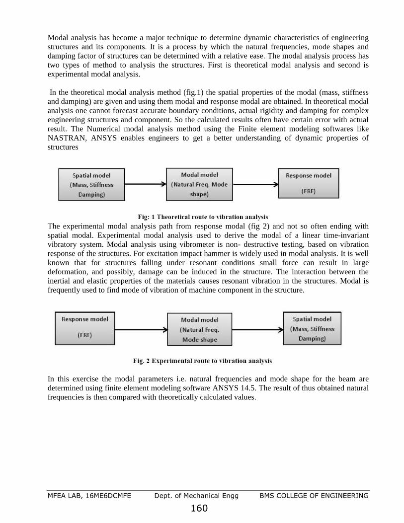
MFEA LAB, 16ME6DCMFE Dept. of Mechanical Engg BMS COLLEGE OF ENGINEERING
160
Modal analysis has become a major technique to determine dynamic characteristics of engineering
structures and its components. It is a process by which the natural frequencies, mode shapes and
damping factor of structures can be determined with a relative ease. The modal analysis process has
two types of method to analysis the structures. First is theoretical modal analysis and second is
experimental modal analysis.
In the theoretical modal analysis method (fig.1) the spatial properties of the modal (mass, stiffness
and damping) are given and using them modal and response modal are obtained. In theoretical modal
analysis one cannot forecast accurate boundary conditions, actual rigidity and damping for complex
engineering structures and component. So the calculated results often have certain error with actual
result. The Numerical modal analysis method using the Finite element modeling softwares like
NASTRAN, ANSYS enables engineers to get a better understanding of dynamic properties of
structures
The experimental modal analysis path from response modal (fig 2) and not so often ending with
spatial modal. Experimental modal analysis used to derive the modal of a linear time-invariant
vibratory system. Modal analysis using vibrometer is non- destructive testing, based on vibration
response of the structures. For excitation impact hammer is widely used in modal analysis. It is well
known that for structures falling under resonant conditions small force can result in large
deformation, and possibly, damage can be induced in the structure. The interaction between the
inertial and elastic properties of the materials causes resonant vibration in the structures. Modal is
frequently used to find mode of vibration of machine component in the structure.
In this exercise the modal parameters i.e. natural frequencies and mode shape for the beam are
determined using finite element modeling software ANSYS 14.5. The result of thus obtained natural
frequencies is then compared with theoretically calculated values.

MFEA LAB, 16ME6DCMFE Dept. of Mechanical Engg BMS COLLEGE OF ENGINEERING
161
II. THEORTICAL MODAL ANALYSIS OF BEAM
2.1 Cantilever beam: fixed - free
Consider an Euler-Bernoulli uniform cantilever beam undergoing transverse vibration condition as
shown in Fig.3.
For free vibrations the equation of motion of beam can be given as [6]

MFEA LAB, 16ME6DCMFE Dept. of Mechanical Engg BMS COLLEGE OF ENGINEERING
162

MFEA LAB, 16ME6DCMFE Dept. of Mechanical Engg BMS COLLEGE OF ENGINEERING
163
Note: Refer appendix on the page No 234

MFEA LAB, 16ME6DCMFE Dept. of Mechanical Engg BMS COLLEGE OF ENGINEERING
164

MFEA LAB, 16ME6DCMFE Dept. of Mechanical Engg BMS COLLEGE OF ENGINEERING
165

MFEA LAB, 16ME6DCMFE Dept. of Mechanical Engg BMS COLLEGE OF ENGINEERING
166

MFEA LAB, 16ME6DCMFE Dept. of Mechanical Engg BMS COLLEGE OF ENGINEERING
167
Steps in a Modal Analysis :
Modal analysis is to determine the vibration characteristics (natural frequencies and mode shapes) of
a structure or a Machine Component while it is being designed. Modal analysis outputs can be used
as input for the following analysis.Transient dynamic analysis,. Harmonic response analysis,
Spectrum analysis.
The procedure for a modal analysis consists of four main steps:
Build the model > Apply loads and obtain the solution > Expand the modes > Review the
results.
Build the model
The geometry can either be created within ANSYS or imported. Only linear behavior is valid in a
modal analysis.Define both Young's modulus (EX) (or stiffness in some form) and density (DENS)
(or mass in some form) for a modal analysis
Apply Loads and Obtain the Solution
Define Analysis Type: Modal
Analysis option

MFEA LAB, 16ME6DCMFE Dept. of Mechanical Engg BMS COLLEGE OF ENGINEERING
168
Choose one of the extraction methods listed below.
Block Lanczos method (default) -used for large symmetric eigenvalue problems. It uses the sparse
matrix solver, overriding any solver specified already
Subspace method -used for large symmetric eigenvalue problems.
When doing a modal analysis with a large number of constraint equations, use the subspace method
with the frontal solver instead of the JCG solver.
The Power Dynamics method -used for very large models (100,000+DOFs), and is especially useful
to .obtain a solution for the first several modes to learn how the model will behave. You can then
choose the most appropriate extraction method (subspace or Block Lanczos) for running the final
solution.
Reduced method is faster than the subspace method because it uses reduced (condensed) system
matrices to calculate the solution. However, it is less accurate because the reduced mass matrix is
approximate.
Unsymmetric method -used for problems with unsymmetrical matrices, such as fluid-structure
interaction problems.
Damped method -used for problems where damping cannot be ignored, such as bearing problems
QR Damped method -faster and achieves better calculation efficiency than the damped method. It
uses the reduced modal damped matrix to calculate complex damped frequencies in modal
coordinates.
For most applications, you will use the Block Lanczos, subspace, reduced, or Power Dynamics
method. The unsymmetric, damped, and QR damped methods are meant for special applications.
Apply Loads
The only "loads" valid in a typical modal analysis are zero-value displacement constraints. You can
specify forces, pressures, temperatures, accelerations, and so on in a modal analysis, but they are
ignored for the mode extraction. However, the program will calculate a load vector and write it to
the mode shape file (Jobname.MODE), so that it can be used in a subsequent mode-superposition
harmonic or transient analysis.
Output
The output from the solution consists mainly of the natural frequencies, which are printed as part of
the printed output (Jobname.OUT) and also written to the mode shape file (Jobname.MODE).The
printed output may include reduced mode shapes and the Participation factor table, depending on
the analysis options and output controls. The mode shapes are not written to the database or to the
results file, so you need to expand the modes to post process the results.
Expand Mode
The term "expansion" means expanding the reduced solution to the full DOF set. The "reduced
solution" is usually in terms of master DOF. In a modal analysis, however, we use the term
"expansion" to mean writing mode shapes to the results file. That is, "expanding the modes" applies
not just to reduced mode shapes from the reduced mode extraction method, but to full mode shapes
from the other mode extraction methods as well. Thus, if you want to review mode shapes in the
postprocessor, you must expand them (that is, write them to the results file).Expanded modes are
also required for subsequent spectrum analyses Number of modes to expand can be defined in many
ways.
Choose Preprocessor > Loads>~ Analysis option. In the Modal Analysis dialog box, enter the "No.
of modes to expand" value;
Or Choose Solution > Load Step Opts > Expansion Pass > Single Expand > Expand Modes
Review the Results
Results from a modal analysis (that is, the model expansion pass) are written to the structural results
file, Job name, RST.
The Results consist of:
Natural frequencies

MFEA LAB, 16ME6DCMFE Dept. of Mechanical Engg BMS COLLEGE OF ENGINEERING
169
Expanded mode shapes
Relative stress and force distributions (if requested)
You can review these results in POST1, the general postprocessor. Some typical post processing
operations for a modal analysis are described below.
Listing All Frequencies
To list the frequencies of all modes expanded, choose General Postproc >List Results
Plotting deformed shape
To define mode shape (deformed shape), choose General Postproc>Plot Results>Deformed Shape
from the Main menu.
Problem 54: Obtain the first ten natural frequencies of the Fixed –Fixed beam shown in
figure and Compare them with theoretical values. Also plot their mode shapes
Modulus of elasticity, E = 2.068x10¹¹ N/m2, Poisson’s ratio, = 0.3, Density, = 7830 kg/m3
M.I of I section = , C/S Area =
Preprocessor
1. Define Element Types
Preprocessor > Element Type > Add/Edit/Delet >Beam>3D Finite Strain > Ok> Options>K3>select Cubic Form. >Ok
2. Define Area: Preprocessor > Sections > Beam >Common Sections > B-0.01, H-0.01 > Ok
3. Define Element Material Properties
Preprocessor >Material Props >Material Models >Structural > Linear >Elastic >
Isotropic, EX: 2.068e11, Poisson’s Ratio, PRXY: 0.3, Density: 7830
4. Preprocessor>Modeling>create>Keypoints>in Active CS
Create 2 Keypoints with the following coordinates
Keypoint X,Y,Z coord.
1 0,0,0
2 1,0,0
5. Preprocessor > Modeling > Create > Lines > Lines > Straight Line
Click on Keypoint 1 and keypoint 2.
6. Preprocessor > Meshing > Size Cntrls > Manual Size > Lines > All Lines. For this example
10 element divisions are specified along the line.
7. Preprocessor > Meshing > Mesh > Lines > Click ‘Pick All’ in the small window appears
8. Solution > Analysis Type > New Analysis > Modal > Ok > Analysis Options
The following window will appear
1.0 m
0.01 m
0.01 m

MFEA LAB, 16ME6DCMFE Dept. of Mechanical Engg BMS COLLEGE OF ENGINEERING
170
Select the PGC lanczos method.
Enter 10 in the ‘No. of modes to extract’
Check the box beside ‘Expand modes shapes’
Enter 10 in the ‘No. of modes to expand’
Click ‘OK’.
The following window will then appear
Keep default options in the above window and click on ‘OK’.
9. Solution>Define Loads>Apply >Structural>Displacement> On Keypoints
Fix all DOFs constraints on Keypoint 1 and click ‘Apply’ in a small window that appears.
Once you click apply in a small window another window will appear, select ‘All DOF’ and click
apply.
Fix keypoint 2 also for fixed-fixed beam and click ‘OK’ in small window.
10. Solution>Solve>Current LS
11. General Postproc > Results Summary …

MFEA LAB, 16ME6DCMFE Dept. of Mechanical Engg BMS COLLEGE OF ENGINEERING
171
The results are compared with theoretical values as shown
Mode Natural Frequencies in Hz Percent Error
Theory ANSYS
1 51.935 52.790 1.7
2 145.654 145.39 0.04
3 285.642 284.68 0.02
12. View Mode Shapes: General Postproc > Read Results > First Set
This select the results for the first mode shape.
General Postproc > Plot Results > Deformed Shapes > Select Def + Undef + edge
The first mode shape is now appear in the graphic window.
To view the next mode shapes, select
General Postproc > Read Results > Next set
General Postproc > Plot Results > Deformed Shapes > Select Def + Undef +edge.
Repeat the above steps for the remaining mode shapes.
13. Animate Mode Shapes: Select Utility Menu (Menu at the top) > Plot Ctrls >Animate
>Mode Shapes. Then the following window will appear.
A
EIa
= where,
3,2,1 Hz 2
1== if ii

MFEA LAB, 16ME6DCMFE Dept. of Mechanical Engg BMS COLLEGE OF ENGINEERING
172
Keeps the default setting and click ‘OK’, animated window will appear
➢ Identify the mode of vibration like axial,bending or torsional
Problem 55: Obtain the first three natural frequencies of the Fixed –Fixed beam shown in
figure and Compare them with theoretical values. Also plot their mode shapes
Modulus of elasticity, E = 2.068x10¹¹ N/m2, Poisson’s ratio, = 0.3, Density, = 7830 kg/m3
Mode Natural Frequencies in Hz Percent
Error
Mode Shape
Theory ANSYS
1
2
3
Problem 56: Obtain the first five natural frequencies of the Fixed –Fixed beam having an I cross
section with a total depth of 150mm, flange width of 100mm, thickness of flange and web being
25mm. Length of the beam is 1000 mm. Also compare with theoretical values
Modulus of elasticity, E = 0.7x10¹¹ N/m2, Poisson’s ratio, = 0.3, Density, = 2700 kg/m3
Mode
Natural Frequencies in Hz Percent
Error
Mode Shape
Theory ANSYS
1
2
3
1.0 m 0.03 m
0.01 m

MFEA LAB, 16ME6DCMFE Dept. of Mechanical Engg BMS COLLEGE OF ENGINEERING
173
Problem 57: Perform Modal Analysis and find first 3 natural frequencies and mode shapes of
the I –Section beam pinned at both ends. Compare the natural frequencies with theorictical ones
E =2.0684 x 10⁵ MPa , = 7850 kg/ mm3 , ν = 0.32
s
Mode Natural Frequencies in Hz Percent
Error
Mode Shape
Theory ANSYS
1
2
3
LUMPED SYSTEMS:
In case of shafts and beams of negligible mass carrying concentrated mass, the force is proportional
to the deflection of the mass from the equilibrium position and the relation derived for natural
frequency of longitudinal vibrations holds good
fn= /21 g
Where EI
mgl
3
3
= for cantilevers, supporting a concentrated mass at the free end.
EI
bmga
3
22
= for simply supported beams
3
33
3 EI
bmga= for beams fixed at both ends

MFEA LAB, 16ME6DCMFE Dept. of Mechanical Engg BMS COLLEGE OF ENGINEERING
174
L
a b
l
a b
l
M M M
Problem 58: A shaft fixed at the ends has a mass of 120kg placed 250 mm from one end.
Determine the frequency of the natural transverse vibrations if the length of the shaft is 700mm, E =
200GPa.and shaft diameter is 40mm. Also compare with theoretical value.
Preprocessor
1. Creation of Fixed Beam used in Modal Analysis:
Give example a Title(optional):Utility Menu > File > Change Title - , Enter Fixed-Fixed Beam
with lumped mass for the title
Give example a Jobname(optional)::Utility Menu > File > Change Jobname - -, Enter Modal_5
for the jobname
2. Define Element Types: Preprocessor > Element Type > Add/Edit/Delete > Add > Beam – 3D
finite strain > Apply > Structural Mass-3D > mass 21> ok.
Pick Type2 MASS21 > options > Rotary inertia options=’2D w/o rot iner’ > ok > Close
3. Real Constants> Add/Edit/Delete > Add >Type 2 MASS21 > ok > 2-D mass = 120
4. Define shaft cross section: Preprocessor > Sections > Common sections > subtype=circular,
R=20, ok
5. Define Element Material Properties: Preprocessor >Material Props >Material Models >
Structural > Linear >Elastic >Isotropic
In the window that appears, enter the following material properties
Young’s Modulus, EX : 200e9
Poisson’s Ratio, PRXY: 0.3
6. Create Nodes:Preprocessor>Modeling>create>Nodes>in Active CS
Create 2 Keypoints with the following coordinates
Keypoint X,Y,Z coord.
1 0,0,0
2 0.25,0,0
3 0.7,0,0
7. Create Elements: Preprocessor>Modeling>create>elements>auto numbered >thru nodes>
pick1&2,2&3>ok> element attributes >element type number= 2Mass21> ok > auto numbered
> thru nodes> pick node 2
8. Solution > Analysis Type > new analysis > modal>ok>
Solution > Analysis Type > Analysis Options
0.7 m
M
0.25

MFEA LAB, 16ME6DCMFE Dept. of Mechanical Engg BMS COLLEGE OF ENGINEERING
175
The following window will appear
Select the Subspace method. Enter 1 in the ‘No. of modes to extract’ Check the box beside ‘Expand
modes shapes’Enter 1 in the ‘No. of modes to expand’
Click ‘OK’.
The following window will then appear
Keep default options in the above window and click on ‘OK’
9. Apply Constraints: Solution > Define Loads>Apply >Structural>Displacement> On Nodes
Fix all DOFs constraints on Nodes1 & 3 and click ok in a small window that appears.
Once you click ok in a small window another window will appear, select ‘All DOF’ and click ok
10. Solve the System: Solution>Solve>Current LS
Post processing
11. Verify Extracted Modes against Theoretical Predictions: General Post proc>Results
Summary
12. View Mode Shapes: General Post proc > Read Results > First Set
This select the results for the first mode shape.
General Postproc > Plot Results > Deformed Shapes > Select Def + Undef + edge
The first mode shape will appear in the graphic window.
Mode Natural Frequencies in Hz Percent
Error
Mode Shape
Theory ANSYS
1
Problem 59: A shaft supported freely at the ends has a mass of 120kg placed 250 mm from one
end. Determine the frequency of the natural transverse vibrations if the length of the shaft is 700mm,
E = 200GPa and shaft diameter is 40mm. Also compare with theoretical value.

MFEA LAB, 16ME6DCMFE Dept. of Mechanical Engg BMS COLLEGE OF ENGINEERING
176
Mode Natural Frequencies in Hz Percent
Error
Mode Shape
Theory ANSYS
1
Problem 60: Obtain the first three natural frequencies of the Fixed –Fixed beam with a
central lumped mass as shown in figure and Compare them with theoretical values. Also plot their
mode shapes.Modulus of elasticity, E = 2.068x10¹¹ N/m2, Poisson’s ratio, = 0.3, Density, = 7830
kg/m3
INA=
Mode Natural Frequencies in Hz Percent
Error
Mode Shape
Theory ANSYS
1
Problem 61: A shaft 40mm diameter and 2.5m long has a mass of 15 kg per meter length.it is
simply supported at the ends and carries three masses 90kg, 140kg and 60kg at 0.8m,1.5m
respectively from the left support . Taking E=200GPa, find the frequency of the transverse
vibrations.
0.8 m
1.5 m
2 m
2.5 m
90 kg 140 kg 60 kg
Hint: In order to account the mass of the shaft, calculate the density of the shaft and use it in material
model.
Analytical Solution:
D =40mm = 0.04m l = 2.5m
1.0 m
0.03 m
0.01 m
M

MFEA LAB, 16ME6DCMFE Dept. of Mechanical Engg BMS COLLEGE OF ENGINEERING
177
( ) 4642 101257.004.06464
mXXXdI −==
27.1
4985.0
111s
nf
+++
= 1 =
EIl
bamgf n
3
22
=
Here m =90kg,a= 0.8m and b=1.7m
mXXXXX
XXX00866.0
5.2101257.0102003
)7.1()8.0(81.99069
22
1 ==−
m =140kg, a= 1.5m b=1m, mXXXXX
XXX1639.0
5.2101257.0102003
)1()5.1(81.914069
22
2 =−
For 3 m =60kg, a= 2m b=0.5m mXXXXX
XXX00312.0
5.2101257.0102003
)5.0()2(81.96069
22
3 ==−
=
mXXXX
XXX
El
mgls 00298.0
101257.010200384
)5.2(81.9155
384
569
44
===−
HzFn 85.2
27.1
00298.000312.001639.000866.0
4985.0=
+++
=
Mode Natural Frequencies in Hz Percent
Error
Mode Shape
Theory ANSYS
1
Note: Refer page no
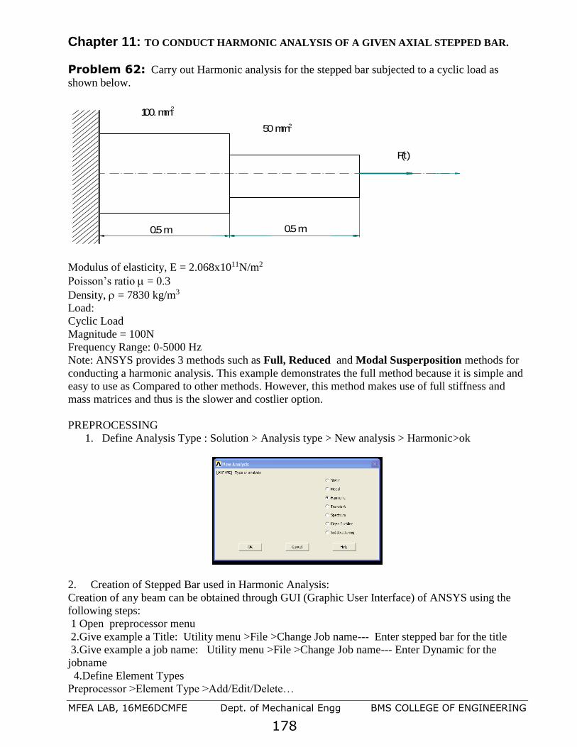
MFEA LAB, 16ME6DCMFE Dept. of Mechanical Engg BMS COLLEGE OF ENGINEERING
178
Chapter 11: TO CONDUCT HARMONIC ANALYSIS OF A GIVEN AXIAL STEPPED BAR.
Problem 62: Carry out Harmonic analysis for the stepped bar subjected to a cyclic load as
shown below.
0.5 m 0.5 m
100. mm
50 mm
2
2
F(t)
Modulus of elasticity, E = 2.068x10¹¹N/m2
Poisson’s ratio = 0.3
Density, = 7830 kg/m3
Load:
Cyclic Load
Magnitude = 100N
Frequency Range: 0-5000 Hz
Note: ANSYS provides 3 methods such as Full, Reduced and Modal Susperposition methods for
conducting a harmonic analysis. This example demonstrates the full method because it is simple and
easy to use as Compared to other methods. However, this method makes use of full stiffness and
mass matrices and thus is the slower and costlier option.
PREPROCESSING
1. Define Analysis Type : Solution > Analysis type > New analysis > Harmonic>ok
2. Creation of Stepped Bar used in Harmonic Analysis:
Creation of any beam can be obtained through GUI (Graphic User Interface) of ANSYS using the
following steps:
1 Open preprocessor menu
2.Give example a Title: Utility menu >File >Change Job name--- Enter stepped bar for the title
3.Give example a job name: Utility menu >File >Change Job name--- Enter Dynamic for the
jobname
4.Define Element Types
Preprocessor >Element Type >Add/Edit/Delete…

MFEA LAB, 16ME6DCMFE Dept. of Mechanical Engg BMS COLLEGE OF ENGINEERING
179
For the problem, the Link (3D Finite stn 180 )element is used. This element has 3 d.o.f (i.e.
translation along X and Y axes and rotation about Z axis)
Define Real constant
Preprocessor >Real Constant .>Add. Enter the following 2 steps geometric properties for elements -
1and 2 For Element 1) Cross sectional area ‘AREA’ for type 1: 0.0001m2 For type 2: 0.0005m2
After entering area 1 0.001 click Apply
After entering area 2 0.00005 click ok
Note : For dynamic analysis the units of area, Young’s modulus density should be in m2 N/m2 and
kg/m3 respectively.
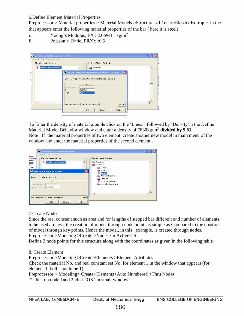
MFEA LAB, 16ME6DCMFE Dept. of Mechanical Engg BMS COLLEGE OF ENGINEERING
180
6.Define Element Material Properties
Preprocessor > Material properties > Material Models >Structural >L1near>Elastic>Isotropic in the
that appears enter the following material properties of the bar ( here it is steel)
i. Young’s Modulus, EX : 2.069e11 kg/m2
ii. Poisson’s Ratio, PRXY :0.3
To Enter the density of material ,double click on the ‘Linear’ followed by ‘Density’in the Define
Material Model Behavior window and enter a density of 7830kg/m3 divided by 9.81
Note : If the material properties of two element, create another new model in main menu of the
window and enter the material properties of the second element .
7.Create Nodes
Since the real constant such as area and /or lengths of stepped bar different and number of elements
to be used are less, the creation of model through node points is simple as Compared to the creation
of model through key points. Hence the model, in this example, is created through nodes.
Preprocessor >Modeling >Create >Nodes>In Active CS
Define 3 node points for this structure along with the coordinates as given in the following table
8. Create Element
Preprocessor >Modeling >Create>Elements >Element Attributes.
Check the material No. and real constant set No. for element 1 in the window that appears (for
element 1, both should be 1)
Preprocessor > Modeling> Create>Elements>Auto Numbered >Thru Nodes
* click on node 1and 2 click ‘OK’ in small window.

MFEA LAB, 16ME6DCMFE Dept. of Mechanical Engg BMS COLLEGE OF ENGINEERING
181
Preprocessor >Modeling >Create>Elements >Element Attributes.
Change the material No. and real constant set No. for element 2 in the window that appears for
element 2,Material No.1 and Real Const.Set No.=2, in this case
Preprocessor > Modeling> Create>Elements>Auto Numbered >Thru Nodes
* click on node 2and 3 click ‘OK’ in small window.
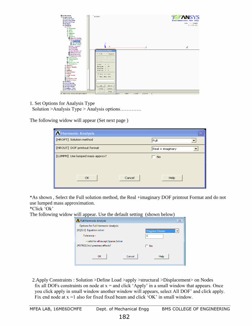
MFEA LAB, 16ME6DCMFE Dept. of Mechanical Engg BMS COLLEGE OF ENGINEERING
182
1. Set Options for Analysis Type
Solution >Analysis Type > Analysis options………….
The following widow will appear (Set next page )
*As shown , Select the Full solution method, the Real +imaginary DOF printout Format and do not
use lumped mass approximation.
*Click ‘Ok’
The following widow will appear. Use the default setting (shown below)
2.Apply Constraints : Solution >Define Load >apply >structural >Displacement> on Nodes
fix all DOFs constraints on node at x = and click ‘Apply’ in a small window that appears. Once
you click apply in small window another window will appears, select All DOF’ and click apply.
Fix end node at x =1 also for fixed fixed beam and click ‘OK’ in small window.

MFEA LAB, 16ME6DCMFE Dept. of Mechanical Engg BMS COLLEGE OF ENGINEERING
183
3.Apply Loads: Solution >Define Loads>apply >structural >force/Moment>on Nodes
select the node at free-end of bar (i.e.at x = 1.0)
The following window will appear. Fill it as shown to apply a load with real value of 100and an
imaginary values of 0 in the positive ‘x’ direction
Note: By specifying a real and imaginary value of the load we are providing information on
magnitude and phase of the load. In this case the magnitude of the load is 100N and its phase is 00
Phase information is most important when we have two or more cyclic loads being applied to the
structure as these load could be in or out phase. For harmonic analysis, all loads must have the same
frequency.
4.Set the Frequency Range Solution >Load Step option >Time/Frequency >Freq and Substps….
As shown in the window below, specify a frequency range of 0-4500Hz 100 Sub steps and stepped
b.c…
5. Solve the System : Solution >Solve Current LS
SOLVE POSTPROCESSING: Viewing the Results
We want to observe the response x = 0.5m (where the load is applied)as a function of frequency. We
cannot do this with General Post processing (POST1),rather we must use Time Hist Post Processing
(POST26).post26 is used to observe certain variable as a function of either time or frequency.
1.Open the Time Hist Processing (POST26)Menu Select Time Hist Postprocessor from the ANSYS
Main Menu

MFEA LAB, 16ME6DCMFE Dept. of Mechanical Engg BMS COLLEGE OF ENGINEERING
184
2. Define Variables
Note: Here we have to define variables that we want to see plotted. By default. Variables 1 is
assigned either Time or Frequency. In this case it assigned frequency, we want to see the
displacement UX at the node at x= 0.5(To get a list of nodes and their attributes. Select Utility
Menu >List Nodes ). Time Hist PostPro >Variable Viewer ………..
The following window will pop up.
• Select Add (the green’+’ sign in the upper left corner)from this window and the following
window will appear.
•
• We are interested in the Nodal Solution >DOF Solution >X-Component. Click OK.
• Graphically select node 2 when promoted and click OK. The ‘Time History Variables
window should now look as follows.

MFEA LAB, 16ME6DCMFE Dept. of Mechanical Engg BMS COLLEGE OF ENGINEERING
185
3 List Stored Variables
In the ‘Time History Variable’ window, click the ‘List’ button (3buttons to left of ‘Add’ button).
The following window will appear listing the data:
4. Plot UX vs Frequency
* in the ‘Time Variable’ window click the ‘Plot’ button (2buttons to the left of ‘Add’ button).
The following graph will be plotted in the main ANSYS window.
Note that we get peaks at frequencies of approximately 1650 and 4250Hz This correspondence with
the predicated natural frequencies of 1627.7and 4220.5Hz respectively during model analysis of the
Same stepped bar.
Obtain the response with log scale of UX similar to the previous case. Then We will now see the
response at free-end of bar for the cyclic load with frequency range 0-5000 Hz as shown below.
Select Utility menu> Plot Ctrl> Style > Graphs > Modify Axes

MFEA LAB, 16ME6DCMFE Dept. of Mechanical Engg BMS COLLEGE OF ENGINEERING
186
Select Utility Menu > Plot > Replot
Problem 63: Conduct harmonic analysis of a given axial stepped bar.
Modulus of elasticity, E = 2.068x10¹¹N/m2
Poisson’s ratio = 0.3
Density, = 7830 kg/m3
Load: Cyclic Load of 300 KN as shown.
Frequency Range: 0-5000 Hz

MFEA LAB, 16ME6DCMFE Dept. of Mechanical Engg BMS COLLEGE OF ENGINEERING
187
Problem 64: Conduct harmonic analysis of a given axial stepped bar.
Modulus of elasticity, E = 2.068x10¹¹N/m2
Poisson’s ratio = 0.3
Density, = 7830 kg/m3
Load: Cyclic Load
Magnitude = 300KN
Frequency Range: 0-800 Hz

MFEA LAB, 16ME6DCMFE Dept. of Mechanical Engg BMS COLLEGE OF ENGINEERING
188
Problem 65: Harmonic analysis of fixed fixed beam
Modulus of elasticity, E = 2.068x10¹¹ N/m2
Poisson’s ratio, = 0.3
Density, = 7830 kg/m3
M.I of I section =8.33e-10 m4
C/S Area=0.0001 m2
Load: cyclic Load
Magnitude, Fo=100 N
Frequency Range = 0 – 300 Hz
1. Define Analysis Type: Solution > Analysis type > New analysis > Harmonic>ok
2. Define Element Types
Preprocessor > Element Type > Add/Edit/Delete For this problem, the BEAM (3D
Finite strain) element is used.
3. Define area: Preprocessor > Sections > Beam >Common Sections B-0.01, H-0.01 > Ok
4. Define Element Material Properties: Preprocessor >Material Props >Material Models >
Structural > Linear >Elastic >Isotropic
In the window that appears, enter the following material properties
Young’s Modulus, EX : 2.068e11
Poisson’s Ratio, PRXY: 0.3
Density : 7830
5. Create Keypoints: Preprocessor>Modeling>create>Keypoints>in Active CS >Create Key points
with the following coordinates
Keypoint X,Y,Z coord.
1 0,0,0
2 1,0,0
6. Define Lines: Preprocessor > Modeling > Create > Lines > Lines > Straight Line Click on
Keypoint 1 and keypoint 2.
7. Define Mesh Size: Preprocessor > Meshing > Size Cntrls > Manual Size > Lines > All Lines .
For this example 10 element divisions are specified along the line.
8. Mesh the Frame: Preprocessor > Meshing > Mesh > Lines > Click ‘Pick All’ in the small
window appears
10. Set Options for Analysis Type
Solution > Analysis Type > Analysis Options . . .
1.0 m
0.01 m
0.01 m
0.5 m F(t)

MFEA LAB, 16ME6DCMFE Dept. of Mechanical Engg BMS COLLEGE OF ENGINEERING
189
The following window will appear
• Select the Full solution method, the Real + imaginary DOF printout format
• Do not use lumped mass approximation.
• Click ‘OK’
Keep default options in the above window and click on ‘OK’.
Apply Constraints: Solution > Define Loads>Apply >Structural>Displacement> On Nodes
Fix all DOFs constraints on Keypoint 1 and Kepoint 2.
Apply Load: Solution > Define Loads > apply > structural > Force/Moment > On Nodes
Select the node at mid-point of the beam (i.e. at x=0.5)
Then the following window will appear.
Fill it as shown to apply a load with real value of 100 and an imaginary value of 0 in the
positive ‘y’ direction.
Set the Frequency Range: Solution > Load Steo Opts > Time/Frequency > Freq and Substps
As shown in the window below, specify a frequency range of 0 – 300 Hz, 300 substeps and
stepped b.c . . .

MFEA LAB, 16ME6DCMFE Dept. of Mechanical Engg BMS COLLEGE OF ENGINEERING
190
11. Solve the System: Solution > Solve > Current LS
12. Open the TimeHist Processing (POST26) Menu
Define Variables : TimeHist PostPro > Variable Viewer . . .
The following window will pop up.
Select Add (the green ‘+’ sign in the upper left corner) from this window and the following window
will appear.
We are interested in the Nodal solution > DOF Solution > Y – Component.
Click OK.
Graphically select node 2 when prompted and click OK.

MFEA LAB, 16ME6DCMFE Dept. of Mechanical Engg BMS COLLEGE OF ENGINEERING
191
13. List Stored Variables: In the ‘Time History Variable’ window, click the ‘List’ button (3rd
buttons to the left of ‘Add’ button).
14. Plot UY vs Frequency: In the ‘Time Variable’ window click the ‘Plot’ button (2nd buttons to
the left of ‘Add’ button).
To get a better view of the response, view the log scale of UY. Select Utility Menu > PlotCtrl >
Style > Graphs > Modify Axis
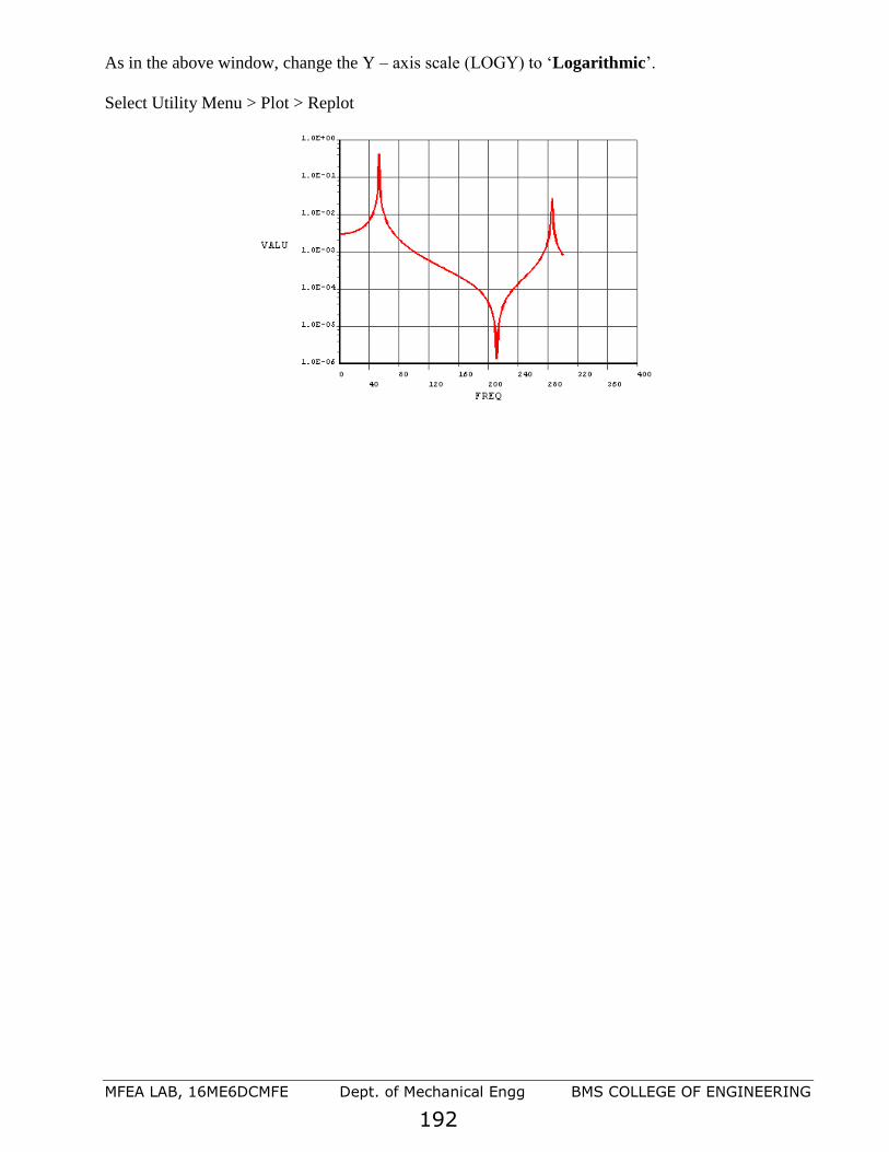
MFEA LAB, 16ME6DCMFE Dept. of Mechanical Engg BMS COLLEGE OF ENGINEERING
192
As in the above window, change the Y – axis scale (LOGY) to ‘Logarithmic’.
Select Utility Menu > Plot > Replot

MFEA LAB, 16ME6DCMFE Dept. of Mechanical Engg BMS COLLEGE OF ENGINEERING
193
Chapter 12: THERMAL ANALYSIS Thermal Analysis:
Practical application: Engine, radiator, exhaust system , heat exchangers, power plants, satellite,design.etc…
Commonly used software’s: Ansys, MD Nastran, Abaqus, I-deas, NX etc….
HEAT TRANSFER: General Steps to be followed while solving a problem by using FEM:
1. Discretize and select the element type
2. Choose a temperature function.
3. Define the temperature gradient / temperature and heat flux/ temperature gradient
relationships.
4. Derive the element conduction matrix and equations by using either variational
approach or by using Galerkin’s approach
5. Assemble the element equations to obtain the global equations and introduce boundary
conditions.
6. Solve for the nodal temperatures
7. Solve for the element temperature gradients and heat fluxes.
HEAT TRANSFER ONE DIMENSIONAL FINITE ELEMENT FORMULATION USING
VARIATIONAL APPROACH STEPS TO BE FOLLOWED:
Step 1. Select element type.
t1
t2
T = N1t1+ N2 t2
1 2
Temperature Variation along the
length of element
t1 t2
1
x
One –D element
L
2

MFEA LAB, 16ME6DCMFE Dept. of Mechanical Engg BMS COLLEGE OF ENGINEERING
194
Step 2. Choose a temperature function.
We choose, T (x) = N1 t1 + N2 t2 --------------------------- (1) Where,
t1 is the temperature at node 1
t2 is the temperature at node 2
N1 & N2 are shape functions given by, L
xN ,
L
x1N
21=−= ------------------- (2)
In matrix form, we write,
)3(t and L
x
L
x1N
2
1−−−−−
=
−=
t
t
Therefore one can express T as )4(−−−−−−= tNT
Step 3. Define the temperature gradient / temperature and heat flux/ temperature gradient
relationships.
The temperature gradient matrix g , similar to strain matrix used in structural analysis is given
by, (5)tBdx
dTg −−−−−−−−−=
=
Where, B is obtained by substituting equation (1) for T(x) into equation (5) and differentiating
w.r.t x, that is,
(6)L
1
L
1
dx
dN
dx
dNB 21 −−−−−−−−−
−=
=
The heat flux /temperature gradient relationship is given by,
(7)gDqx −−−−−−−−−−=
Where the material property matrix is now given by,
)8(−−−−−−−−= xxKD
Step 4. Derive the element conduction matrix and equations.
Consider the following equations.
(I)0Qdx
TdK
2
2
xx −−−−−−−−=+
With T =TB on surface S1, 2xx
*
x SonConstantdx
dTKq =−=
L
T=TB
S1
q x = + q*x
S2
q x = 0
L
T=TB
S1
Insulated

MFEA LAB, 16ME6DCMFE Dept. of Mechanical Engg BMS COLLEGE OF ENGINEERING
195
Where, Q is heat generated / unit volume and *
xq is the heat flow / unit area
*
xq is positive when heat is flowing into body
is negative when heat is flowing out of the body
is Zero on an insulated boundary.
And ( ) (II)TTA
hP
t
TCρQ
x
TK
xxx −−−−−−−+
=+
With the first boundary condition of above equation and /or second boundary condition and /or loss
of heat by convection from the ends of 1-D body.
We have,
( ) 3xx SsurfaceonTThdx
dTK −=−
Above equations can be shown to be derivable by the minimization of the following functional
(analogous to the potential energy functional π)
IIIΩΩΩUΠ hqQh −−−−−−−−−−−+++=
Where,
dVdx
dTK
2
1U
v
2
xx
= , −=
V
Q dVTQΩ , −=2S
* dSTqΩq and
( ) )9(2
1Ω
2
h
3
−−−−−−−−−−−= dSTThS
(q* and h on the same surface cannot be specified simultaneously because they cannot occur on the
same surface)
Therefore,
Insulated
h
T T

MFEA LAB, 16ME6DCMFE Dept. of Mechanical Engg BMS COLLEGE OF ENGINEERING
196
( ) )10(dSTTh2
1dSTqdVTQdV
dx
dTK
2
1
ΩΩΩUΠ
2
SS
*
Vv
2
xx
hqQh
32
−−−−−+−−
=
+++=
Consider the first term of equation (10),
)11(2
1dV
dx
dTK
2
1
v
2
xx −−−−−−−−−=
dVgDgV
T
Consider the second term of equation (10),
(12)-------dVTQV
dVQNtV
TT
=
Third term of equation (10) gives,
(13)dSqNtdSTq *T
S
T
S
*
22
−−−−−−−=
Fourth term gives,
( ) )14(2
1
2
1 22
33
−−−−−−−−=− dSTNthdSTTh
S
TT
S
Substituting equations (11),(12),(13) and (14) in equation (10) we obtain
( ) (15)dSTTtNNttNNth2
1
dS*qNtdVQNttdVBDBt2
1
dSTNth2
1dSqNt
dVgDg2
1Π
3
2
32
S
2TTTT
T
S
TT
V
TT
V
T
2
S
TT*T
S
T
V
T
h
−−−++−+
−−=
−+−
−=
dVQNtV
TT
In equation (15), the
minimization is most easily accomplished by explicitly writing the surface integral S3 with t , left
inside the integral as shown.
On minimizing equation (15) w.r.t. t , we get
)16(0dShTNtdSNNh
dS*qNdVQNtdVBDBt
Π
3 3
2
S S
TT
T
S
T
V
T
V
h
−−−−−−−=−+
−−=
On simplifying,
(17)ffftdSNNhdVBDBhqQ
S
TT
V 3
−−−−++=
+
Where the force matrices have been defined by,
Equation (17) can be written in the form (18)tKf −−−−−−−−=
===
32 S
T
h
T
S
q
T
V
QdShTNf,dS*qNf,dVQNf
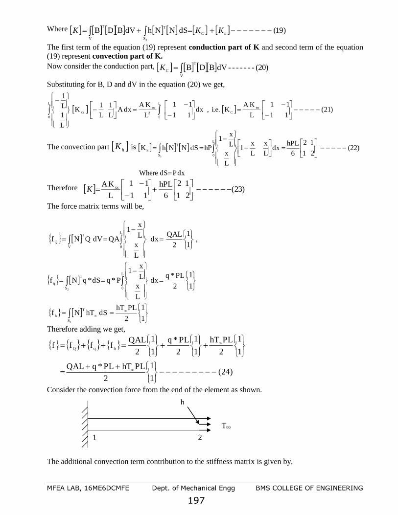
MFEA LAB, 16ME6DCMFE Dept. of Mechanical Engg BMS COLLEGE OF ENGINEERING
197
Where )19(dSNNhdVBDB3S
TT
V
−−−−−−−+=+= hCKKK
The first term of the equation (19) represent conduction part of K and second term of the equation
(19) represent convection part of K.
Now consider the conduction part, (20)-------dVBDBT
V
=CK
Substituting for B, D and dV in the equation (20) we get,
)21(11
11
L
KAKi.e. ,dx
11
11
L
KAdxA
L
1
L
1K
L
1
L
1
xx
C
L
02
xx
xx
L
0
−−−−−
−
−=
−
−=
−
−
The convection part h
K is
dxPdSWhere
(22)21
12
6
hPLdx
L
x
L
x1
L
x
L
x1
hPdSNNhKL
0S
T
h
3
=
−−−−−
=
−
−
==
Therefore )23(21
12
6
hPL
11
11
L
KAxx −−−−−−
+
−
−=K
The force matrix terms will be,
==
=
−
==
=
−
==
1
1
2
PLhTdShTNf
1
1
2
PL*qdx
L
x
L
x1
P*qdS*qNf
,1
1
2
QALdx
L
x
L
x1
QAdVQNf
3
2
S
T
h
L
0
T
S
q
L
0
T
V
Q
Therefore adding we get,
)24(1
1
2
PLhTPL*qQAL
1
1
2
PLhT
1
1
2
PL*q
1
1
2
QALffff
hqQ
−−−−−−−−−
++
=
+
+
=++=
Consider the convection force from the end of the element as shown.
The additional convection term contribution to the stiffness matrix is given by,
1 2
h
T00

MFEA LAB, 16ME6DCMFE Dept. of Mechanical Engg BMS COLLEGE OF ENGINEERING
198
(25)dSNNhKendS
T
endh−−−−−−−=
N1 = 0 and N2 = 1 at right end and
(26)10
00hAdS10
1
0hK
endS
endh−−−−−−−
=
=
The convection force from the free end of the element is obtained from the application of equation of
h
f with the shape function now evaluated at the right end and with S3 ( the surface over which
convection occurs) now equal to the c/s area A of the rod.
Step 5. Assemble the element equations to obtain the global equations and introduce boundary
conditions.
The global structure conduction matrix is
=
=n
e
eKK1
The global force matrix is
=
=n
1e
efF
and global equations are
tKF =
Step 6. Solve for the nodal temperatures
Step 7. Solve for the element temperature gradients and heat fluxes.
ONE DIMENSIONAL FINITE ELEMENT FORMULATION USING GALERKIN’S
APPROACH
Equation representing one dimensional formulation of conduction with convection is given by,
( ) (1)TTA
hPQ
dx
Tdk
2
2
x−−−−−−−=+
To derive the finite element equations, a two-noded linear element with the temperature function T (x) = N1 t1 + N2 t2 --------------------------- (2) is considered
The residual equations for the equation (I) are expressed as,
)26(1
0AhT
)(
)(AhTf
2
1
h−−−−−−
=
=
==
LxN
LxNend

MFEA LAB, 16ME6DCMFE Dept. of Mechanical Engg BMS COLLEGE OF ENGINEERING
199
( ) (3)0dxANTTA
hPQ
dx
Tdk
i
x
x2
2
x
2
1
−−−−−−=
−−+
Where i = 1,2
Or
(4)0dxNThPdxNQAdxNThPdxNdx
TdkA
2
1
2
1
2
1
2
1
x
x
x
x
i
x
x
i
x
x
ii2
2
x−−−−−−=++−
Where i
= 1,2
Integrating the first term of equation (4) by parts and rearranging, we get
)5(dx
dTANKdxNThPdxNQAdxNThPdx
dx
dT
dx
dNAk
2
1
2
1
2
2
2
1
2
1
x
x
x
x
x
x
ixi
x
x
ii
x
x
i
x−++=+
Where i = 1,2
Substituting for T from equation (2) we obtain,
)6(dx
dTANKdxNThPdxNQA
dxtNtNNhPdxtdx
dNt
dx
dN
dx
dNAk
2
1
2
2
2
1
2
1
2
1
x
x
x
x
ixi
x
x
i
x
x
2211i2
2
1
1
x
x
i
x
−−++=
++
+
The two equations represented by the equation (6) are conveniently combined into a matrix form by
rewriting equation (1) as,
(7)tNt
tNNT(x)
2
1
21−−−−−=
=
and substituting to obtain,
(8)dx
dTNAKdxNThPdxNQA
dxtNNhPdxtdx
dN
dx
dNAk
2
1
2
2
2
1
2
1
2
1
x
x
x
x
T
x
Tx
x
T
x
x
T
Tx
x
x
−−++=
+
The above equation now can be written in the desired finite element form as,
(9)ffftk e
h
e
q
e
Q
e −−−−−−++=

MFEA LAB, 16ME6DCMFE Dept. of Mechanical Engg BMS COLLEGE OF ENGINEERING
200
Where ek is the conductance matrix defined as
)10(dxNNhPdxdx
dN
dx
dNAkk
2
1
2
1
x
x
T
Tx
x
x
e −−−−+
=
First term of the above equation represents the conductance part where as the second term
convection part of the conduction matrix.
Let x1= 0 and x2 = L, then,
N1 & N2 are shape functions given by, L
xN ,
L
x1N 21 =−= ------------------- (11)
If one substitute for N1 & N2 in equation (10) and solve then ek is given by,
(12)kk21
12
6
hPL
11
11
L
kAk e
h
e
c
xe −−−−−−+=
+
−
−=
The forcing function vectors on the right hand side of the equation (8) are given by
=
=
1
1
2
QALAf
0
2
0
1
e
Q L
L
dxQN
dxQN
=
=
−
==
=
2
1
Lx
0x
L
0
x
e
qq-
qA
q-
qA
dx
dT
dx
dT
Akf Where q1 and q2 are the boundary fluxes at
nodes 1 and 2 respectively.
)13(1
1
2
PLhTPhTf
0
2
0
1
h−−−−−−−
=
=
L
L
dxN
dxN

MFEA LAB, 16ME6DCMFE Dept. of Mechanical Engg BMS COLLEGE OF ENGINEERING
201
LINK33: 3-D Conduction33 Bar
LINK33 is a uniaxial element with the ability to conduct heat between its nodes. The element has a
single degree of freedom, temperature, at each node point. The conducting bar is applicable to a
steady-state or transient thermal analysis. If the model containing the conducting bar element is also
to be analyzed structurally, the bar element should be replaced by an equivalent structural element
The conducting bar is applicable to a 3-D (plane or axisymmetric), steady-state or transient thermal
analysis.
LINK33 Input Data The element is defined by two nodes, a cross-sectional area, and the material properties. Specific
heat and density are ignored for steady-state solutions. The thermal conductivity is in the element
longitudinal direction.
Element loads are described in Nodal Loading. Heat generation rates may be input as element body
loads at the nodes. The node J heat generation rate HG(J) defaults to the node I heat generation rate
HG(I).
Element loads are described in Node and Element Loads. Heat generation rates may be input as
element body loads at the nodes. The node J heat generation rate HG(J) defaults to the node I heat
generation rate HG(I).
LINK33 Input Summary
Nodes I, J
Degrees of Freedom TEMP
Real Constants AREA - Cross-sectional area
Material Properties KXX, DENS, C, ENTH
Surface Loads None
Body Loads Heat Generation -- HG(I), HG(J)
LINK33 Output Data
The solution output associated with the element is in two forms:
• Nodal temperatures included in the overall nodal solution
• Additional element output as shown in Table: "LINK33 Element Output Definitions"
The Element Output Definitions table uses the following notation:
A colon (:) in the Name column indicates the item can be accessed by the Component Name method
[ETABLE, ESOL]. The O column indicates the availability of the items in the file Jobname.OUT.
The R column indicates the availability of the items in the results file.
In either the O or R columns, Y indicates that the item is always available, a number refers to a table
footnote that describes when the item is conditionally available, and a - indicates that the item is not
available.

MFEA LAB, 16ME6DCMFE Dept. of Mechanical Engg BMS COLLEGE OF ENGINEERING
202
Table LINK33 Element Output Definitions
Name Definition O R
EL Element Number Y Y
NODES Nodes - I, J Y Y
MAT Material Y Y
VOLU: Volume Y Y
XC, YC Location where results are reported Y 1
LENGTH Length Y Y
AREA Input area Y Y
TEMP(I, J) Temperatures - I, J Y Y
HEAT RATE Heat flow rate from node I to node J Y Y
THERMAL FLUX Thermal flux (heat flow rate/cross-sectional area) Y Y
Name output quantity as defined in the Table: "LINK33 Element Output Definitions"
Item
predetermined Item label for ETABLE command
E sequence number for single-valued or constant element data
Table LINK33 Item and Sequence Numbers
Output Quantity Name ETABLE and ESOL Command Input
Item E
HEAT RATE SMISC 1
TEMPI SMISC 2
TEMPJ SMISC 3
THERMAL FLUX SMISC 4
LENGTH NMISC 1
AREA NMISC 2
LINK34: Convection34
LINK34 Element Description
LINK34 is a uniaxial element with the ability to convect heat between its nodes. The element has a
single degree of freedom, temperature, at each node point. The convection element is applicable to a
2-D (plane or axisymmetric) or 3-D, steady-state or transient thermal analysis.
If the model containing the convection element is also to be analyzed structurally, the convection
element should be replaced by an equivalent (or null) structural element.

MFEA LAB, 16ME6DCMFE Dept. of Mechanical Engg BMS COLLEGE OF ENGINEERING
203
LINK34 Input Data
The geometry and node locations for this convection element are shown in Figure "LINK34
Geometry". The element is defined by two nodes, a convection surface area, two empirical terms,
and a film coefficient. In an axisymmetric analysis the convection area must be expressed on a full
360° basis. The empirical terms n (input as EN) and CC determine the form of the convection
equation in conjunction with KEYOPT(3).The convection function is defined as follows:
q = hf*A*E*(T(I) - T(J)) where:
q = heat flow rate (Heat/Time)
hf = film coefficient (Heat/Length2*Time*Deg)
A = area (Length2)
T = temperature (this substep) (Deg)
E = empirical convection term = F*ITp(I) - Tp(J)In + CC/hf
Tp = temperature (previous substep) (Deg)
n = empirical coefficient (EN)
CC = input constant
LINK34 Input Summary Nodes I, J
Degrees of Freedom TEMP
Real Constants
AREA - Convection surface area
EN - Empirical coefficient
CC - Input constant
Material Properties HF
Surface Loads Convections --
Body Loads Heat Generation -- HG(I), HG(J)
LINK34 Output Data The solution output associated with the element is in two forms:
• Nodal temperatures included in the overall nodal solution
• Additional element output as shown in Table 34.1: "LINK34 Element Output Definitions"
The heat flow rate is in units of Heat/Time and is positive from node I to node J. In an axisymmetric
analysis, the heat flow is on a full 360° basis. A general description of solution output is given in
Solution Output. See the Basic Analysis Guide for ways to view results.

MFEA LAB, 16ME6DCMFE Dept. of Mechanical Engg BMS COLLEGE OF ENGINEERING
204
The Element Output Definitions table uses the following notation:
A colon (:) in the Name column indicates the item can be accessed by the Component Name method
[ETABLE, ESOL]. The O column indicates the availability of the items in the file Jobname.OUT.
The R column indicates the availability of the items in the results file.
In either the O or R columns, Y indicates that the item is always available, a number refers to a table
footnote that describes when the item is conditionally available, and a - indicates that the item is not
available.
Table 34.1 LINK34 Element Output Definitions
Name Definition O R
EL Element Number Y Y
NODES Nodes - I, J Y Y
XC, YC Location where results are reported Y 1
H Film coefficient (includes empirical term) Y Y
AREA Input area Y Y
TEMP Temperature at node I and node J Y Y
HEAT RATE Heat flow rate from node I to node J Y Y
Table LINK34 Item and Sequence Numbers
Output Quantity Name ETABLE and ESOL Command Input
Item E I J
HEAT RATE SMISC 1 - -
TEMP SMISC - 2 3
H NMISC 1 - -
AREA NMISC 2 - -
LINK34 Assumptions and Restrictions
• If Tp(I) = Tp(J) and n are nonzero, the first term of E is defined to be zero.
• Since all unspecified nodal temperatures are initially set to the uniform temperature, a
nonzero value of n may result in no heat flowing through the element in the first substep of a
thermal solution.
• Nodes may or may not be coincident.
• The element is nonlinear if n is nonzero or KEYOPT(3) = 3. However, the solver always
assumes the element is nonlinear and, therefore, always performs an iterative solution. (Only
2 iterations are performed if the element is linear.)

MFEA LAB, 16ME6DCMFE Dept. of Mechanical Engg BMS COLLEGE OF ENGINEERING
205
Problem 66: For the composite wall idealized by the 1-D model shown in figure below,
determine the interface temperatures. For element 1, let K1 = 5 W / m 0C, for element 2, K2 = 10 W /
m 0C and for element 3, K3 = 15 W / m 0C. The left end has a constant temperature of 200 0C and the
right end has a constant temperature of 600 0C.
`
Solution:
Given:
Finite Element model:
Step 1- Ansys Utility Menu
File -Clear and start new -Do not read file -ok
File -Change job name -Enter new job name -probl –ok
File -Change title -Enter new title -yyy –ok
Step 2 -Ansys Main Menu -Preferences
Select -THERMAL -ok
Step 3 -Preprocessor
Element Type -Add/Edit/Delete -Add- LINK>3D CONDUCTION -33- ok -close
Real constants - Add/Edit/Delete-Add-type 1-link 33- real constant set no 1 – cross sectional area –
enter -0.1-ok-close
Material properties – Material models – material model number 1-thermal – conductivity –
isotropic - conductivity for material - thermal conductivity (Kxx) –5 -ok- material –new model –
define material ID -2-ok- thermal – conductivity –isotropic - conductivity for material - thermal
conductivity (Kxx) –10 –ok- material –new model – define material ID -3-ok- thermal – conductivity
–isotropic - conductivity for material - thermal conductivity (Kxx) –15 –ok-close
Preprocessor-Modeling -Create -Nodes -in active CS -x,y,z location in CS-0,0,0 (x,y value w.r.t
first node)- apply ( first node is created )- 0.1,0,0 -apply ( second node is created) -0.2,0,0 –apply (
third node is created)- 0.3,0,0 -apply ( fourth node is created) -ok
Create –elements-element attributes-select material number-1-real constant set number -1-Auto
numbered – thru nodes – pick 1, 2 (element 1 is created)-ok - element attributes-select material
t1 = 200 0C t4 = 200 0C A = 0.1 m2
K1= 5 W / m 0C K2= 10 W / m 0C K3= 15 W / m 0C
T= 200 0C
0.1 m 0.1 m 0.1 m
1 2 3
T= 600 0C A= 0.1 m2
1 2 3 4
0.1 m 0.1 m 0.1 m
t1 t2 t3 t4
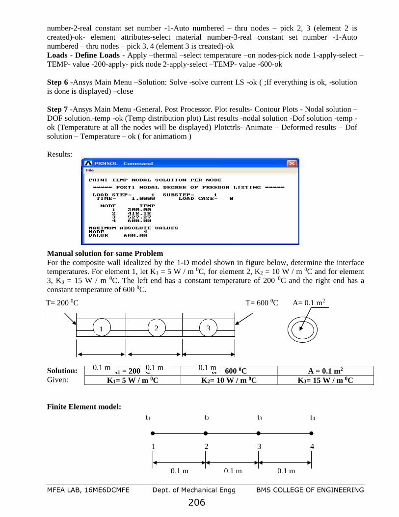
MFEA LAB, 16ME6DCMFE Dept. of Mechanical Engg BMS COLLEGE OF ENGINEERING
206
number-2-real constant set number -1-Auto numbered – thru nodes – pick 2, 3 (element 2 is
created)-ok- element attributes-select material number-3-real constant set number -1-Auto
numbered – thru nodes – pick 3, 4 (element 3 is created)-ok
Loads - Define Loads - Apply –thermal –select temperature –on nodes-pick node 1-apply-select –
TEMP- value -200-apply- pick node 2-apply-select –TEMP- value -600-ok
Step 6 -Ansys Main Menu –Solution: Solve -solve current LS -ok ( ;If everything is ok, -solution
is done is displayed) –close
Step 7 -Ansys Main Menu -General. Post Processor. Plot results- Contour Plots - Nodal solution –
DOF solution.-temp -ok (Temp distribution plot) List results -nodal solution -Dof solution -temp -
ok (Temperature at all the nodes will be displayed) Plotctrls- Animate – Deformed results – Dof
solution – Temperature – ok ( for animatiom )
Results:
Manual solution for same Problem
For the composite wall idealized by the 1-D model shown in figure below, determine the interface
temperatures. For element 1, let K1 = 5 W / m 0C, for element 2, K2 = 10 W / m 0C and for element
3, K3 = 15 W / m 0C. The left end has a constant temperature of 200 0C and the right end has a
constant temperature of 600 0C.
`
Solution:
Given:
Finite Element model:
t1 = 200 0C t4 = 600 0C A = 0.1 m2
K1= 5 W / m 0C K2= 10 W / m 0C K3= 15 W / m 0C
T= 200 0C
0.1 m 0.1 m 0.1 m
1 2 3
T= 600 0C A= 0.1 m2
1 2 3 4
0.1 m 0.1 m 0.1 m
t1 t2 t3 t4

MFEA LAB, 16ME6DCMFE Dept. of Mechanical Engg BMS COLLEGE OF ENGINEERING
207
Element conduction matrices are,
2R
1R
55
55
2C1C
11
11
0.1
50.1X
11
11
L
KAk
1
111
−
−=
−
−=
−
−=
3R
2R
0101
0101
3C2C
11
11
0.1
010.1X
11
11
L
KAk
2
222
−
−=
−
−=
−
−=
R4
3R
5151
5151
4C3C
11
11
0.1
510.1X
11
11
L
KAk
3
333
−
−=
−
−=
−
−=
And the global structure conduction matrix is,
4R
3R
R2
1R
151500
1525100
010155
0055
4C3C2C1C
4R
3R
R2
1R
151500
151510100
0101055
0055
4C3C2C1C
K
−
−−
−−
−
=
−
−+−
−+−
−
=
Now the global equations are given by, FtK = That is,
=
−
−−
−−
−
2
1
4
3
2
1
F
0
0
F
t
t
t
t
151500
1525100
010155
0055
Since the values of t1 and t4 are specified, the equations are modified as follows.
We have now two equations and two unknowns since t1 and t4 are specified.
900025t10t
100010t15t
32
32
=+−
=−
On solving for t2 and t3 we get t3 = 527.3 0C and t2 = 418.2 0C
C600C527.3C418.2C200tTherefore, 0000T=
From ANSYS it was
C600C527.27C418.18C200t 0000T=

MFEA LAB, 16ME6DCMFE Dept. of Mechanical Engg BMS COLLEGE OF ENGINEERING
208
Prob1em 67: A furnace wall is made of inside silica brick (K=1.5 W /mK) and outside
magnesia brick (k=4.9W/mK), each 10cm thick. The inner and outer surfaces are exposed to fluids
at temperatures of 820oC and 110 oC respectively. The contact resistance is 0.001m2 K/W the heat
transfer co-efficient for inner and outer surfaces is equal to 35W/m2 K. Find the heat flow through
the wall per unit area per unit time and temperature distribution across the wall
T1
h1
k1
T2 T3
L1
k3
T4 T5
L3
T6
L2
h4
k2
k1
k3
L1
T1
T6
h1 h4=L2
Rc
k2 A=
Rc
==
====1.5 W /mK
4.9 W/mKL3 = 100mm
8200C
1100C0.001m K/W
2
=35W/m K2
Take L2
k2
A
= 1mm,==
1 W/mK1m2
For FE model,
T1 T2 T3 T4 T5 T6
1 2 3 4 5
Element No. Element Type
2, 3, 4 LINK 33
1, 5 LINK 34
Step 1- Ansys Utility Menu
File -Clear and start new -Do not read file -ok
File -Change job name -Enter new job name –problem60 –ok
File -Change title -Enter new title -yyy –ok
Step 2 -Ansys Main Menu -Preferences
Select -THERMAL -ok
Step 3 -Preprocessor
Element Type -Add/Edit/Delete -Add- LINK -3 D CONDUCTION -33- apply –CONVECTION 34
– ok - close
Real constants - Add/Edit/Delete-Add-select-type 1-link 33- real constant set no 1 – cross sectional
area –enter -1-ok-close – Add-Select- Type 2 Link 34 – Real Constant Set No. 2 – Cross Sectional
area – enter – 1 – ok – close.
Material properties – Material models – material model number 1-thermal – conductivity –
isotropic - conductivity for material - thermal conductivity (Kxx) –1.5 -ok- material –new model –
define material ID -2-ok- thermal – conductivity –isotropic - conductivity for material - thermal
conductivity (Kxx) –1 –ok- material –new model – define material ID -3-ok- thermal – conductivity –
isotropic - conductivity for material - thermal conductivity (Kxx) –4.9 –ok- material –new model –
define material ID -4-ok- thermal – convection or film coef. –enter HF =35 –ok – close.
Step 4: Modelling
Preprocessor-Modeling -Create -Nodes -in active CS -x,y,z location in CS-0,0,0 (x,y value w.r.t
first node)- apply ( first node is created )- 0.001,0,0 -apply ( second node is created) -0.101,0,0 –
apply ( third node is created)- 0.102,0,0 -apply ( fourth node is created) -0.202,0,0 -apply ( fifth
node is created) -0.203,0,0 -apply ( last or sixth node is created) ok

MFEA LAB, 16ME6DCMFE Dept. of Mechanical Engg BMS COLLEGE OF ENGINEERING
209
Create –elements-element attributes-select element type number – LINK34- material number-4-
real constant set number -2-Auto numbered – thru nodes – pick 1, 2 (element 1 is created)-ok -
element attributes-select element type number – LINK33 - material number-2-real constant set
number -1-Auto numbered – thru nodes – pick 2, 3 (element 2 is created)-ok- element attributes-
select element type number – LINK33 - material number-3-real constant set number -1-Auto
numbered – thru nodes – pick 3, 4 (element 3 is created)-ok - element attributes-select element
type number – LINK33 - material number-4-real constant set number -1-Auto numbered – thru
nodes – pick 4, 5 (element 4 is created)-ok - element attributes-select element type number –
LINK34 - material number-4-real constant set number -2-Auto numbered – thru nodes – pick 5, 6
(element 5 is created)-ok.
Step 5 : Solution:- Analysis Type – New Analysis – pick Steady State – ok.
Loads - Define Loads - Apply –thermal –select temperature –on nodes-pick node 1-apply-select –
TEMP- value -820-apply- pick node 6-ok-select –TEMP- value -110-ok
Step 6 -Ansys Main Menu –Solution: Solve -solve current LS -ok (If everything is correct, -
solution is done is displayed) –close
Step 7 -Ansys Main Menu -General. Post Processor, Plot results- Contour Plots - Nodal solution –
DOF solution.-temp -ok (Temp distribution plot) Plotctrls- Animate – Deformed results – Dof
solution – Temperature – ok ( for animatiom ) List results -nodal solution -Dof solution -temp -ok
(Temperature at all the nodes will be displayed)
PRINT TEMP NODAL SOLUTION PER NODE ***** POST1 NODAL DEGREE OF FREEDOM LISTING *****
LOAD STEP= 1 SUBSTEP= 1
TIME= 1.0000 LOAD CASE= 0
NODE TEMP
1 820.00
2 680.31
3 354.36
4 349.47
5 249.69
6 110.00
MAXIMUM ABSOLUTE VALUES
NODE 1
VALUE 820.00
Element Table – Define Table – Add – enter Lab = Heat Flow – Select By Seqeunce Num -
SMISC – SMISC, 1 – ok.
Element Table – List Elem Table – Select Heat Flow – ok. (Heat flow is displayed). PRINT ELEMENT TABLE ITEMS PER ELEMENT ***** POST1 ELEMENT TABLE LISTING *****
STAT CURRENT
ELEM HEATFLOW
1 4889.2
2 4889.2
3 4889.2
4 4889.2
5 4889.2
MINIMUM VALUES
ELEM 2
VALUE 4889.2
MAXIMUM VALUES
ELEM 4
VALUE 4889.2
Note: Refer appendix on the page No 234
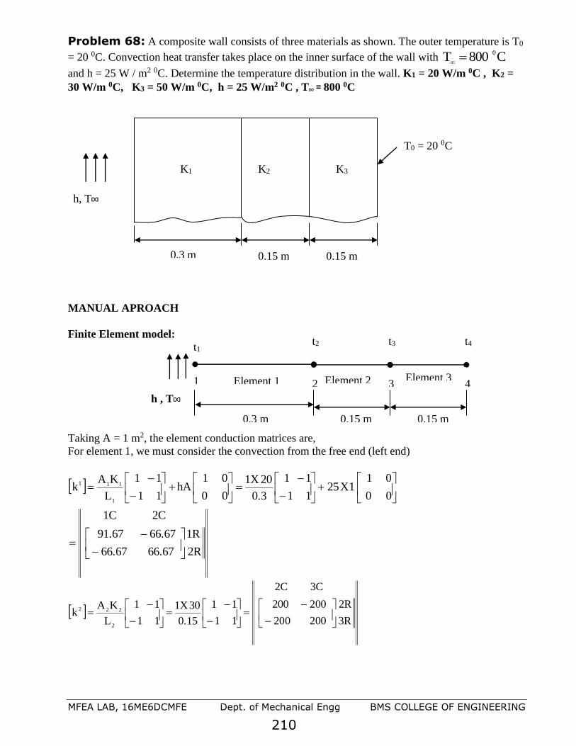
MFEA LAB, 16ME6DCMFE Dept. of Mechanical Engg BMS COLLEGE OF ENGINEERING
210
Problem 68: A composite wall consists of three materials as shown. The outer temperature is T0
= 20 0C. Convection heat transfer takes place on the inner surface of the wall with C800T 0=
and h = 25 W / m2 0C. Determine the temperature distribution in the wall. K1 = 20 W/m 0C , K2 =
30 W/m 0C, K3 = 50 W/m 0C, h = 25 W/m2 0C , T∞ = 800 0C
MANUAL APROACH
Finite Element model:
Taking A = 1 m2, the element conduction matrices are,
For element 1, we must consider the convection from the free end (left end)
2R
1R
66.6766.67
66.6791.67
2C1C
00
011X25
11
11
0.3
201X
00
01hA
11
11
L
KAk
1
111
−
−=
+
−
−=
+
−
−=
3R
2R
002020
002200
3C2C
11
11
0.15
301X
11
11
L
KAk
2
222
−
−=
−
−=
−
−=
h , T∞
1 2 3 4
0.3 m 0.15 m 0.15 m
t1 t2 t3 t4
Element 1 Element 2 Element 3
K1 K2 K3
0.3 m 0.15 m 0.15 m
h, T∞
T0 = 20 0C

MFEA LAB, 16ME6DCMFE Dept. of Mechanical Engg BMS COLLEGE OF ENGINEERING
211
R4
3R
33.33333.333
33.33333.333
4C3C
11
11
0.15
501X
11
11
L
KAk
3
333
−
−=
−
−=
−
−=
And the global structure conduction matrix is,
4R
3R
R2
1R
33.33333.33300
33.33333.5332000
020067.26667.66
0067.6667.91
4C3C2C1C
4R
3R
R2
1R
33.33333.33300
33.33333.3332002000
020020067.6667.66
0067.6667.91
4C3C2C1C
K
−
−−
−−
−
=
−
−+−
−+−
−
=
Now the global equations will be in the form,
FtK =
And end)(leftfendh
is
2R
1R
0
AhT
1C
0
AhT
0
1AhTf
h
=
=
=
Therefore,
=
−
−−
−−
−
44
3
2
1
F
0
0
hT
t
t
t
t
33.33333.33300
33.33333.5332000
020067.26667.66
0067.6667.91 A
Since h, T∞ and t4 are specified, the above equations are modified as,
We now obtain three sets of simultaneous equations in which we have three unknown temperatures.

MFEA LAB, 16ME6DCMFE Dept. of Mechanical Engg BMS COLLEGE OF ENGINEERING
212
6.666633.533200
020067.26667.66
2000067.6667.91
32
321
21
=+−
=−+−
=−
tt
ttt
tt
On solving, we get C14.75tC,119.05tC,304.76t 0
3
0
2
0
1===
The temperatures are,
C20 C14.75C119.05C304.76t 0000T=
COMPARE WITH ANSYS RESULTS
Problem 69: The fin shown in figure is insulated on the perimeter. The left end has a constant
temperature of 100 0C. A positive heat flux q*= 5000 W / m2 acts on the right end. Let Kxx = 6 W/
m0C and cross sectional area A = 0.1 m2. Determine the temperatures at Land4
3L,
2
L,
4
L. Where
L = 0.4 m.
Solution:
Finite Element model:
Element conduction matrices are,
T= 100 0C
L = 0.4 m
q = 5000 W/ m2
Given: t1 = 100 0 C, Kxx = 6 W / m 0 C, A = 0.1 m2
L1 = L2 = L3 = L4 = 0.1 m
T= 100 0C
L = 0.1 m
q = 5000 W/ m2
L = 0.1 m L = 0.1 m L = 0.1 m
t1 t2 t3 t4 t5

MFEA LAB, 16ME6DCMFE Dept. of Mechanical Engg BMS COLLEGE OF ENGINEERING
213
CW/2R
1R
66
66
2C1C
11
11
0.1
60.1X
11
11
L
KAk 0
1
111
−
−=
−
−=
−
−=
Similarly we have
CW/3R
2R
66
66
3C2C
k 02
−
−= , CW/
4R
3R
66
66
4C3C
k 03
−
−= and
CW/5R
4R
66
66
5C4C
k 04
−
−=
and the global structure conduction matrix is,
CW/
5R
4R
3R
R2
1R
66000
612600
061260
006126
00066
5C4C3C2C1C
5R
4R
3R
R2
1R
66000
666600
066660
006666
00066
5C4C3C2C1C
K
0
−
−−
−−
−−
−
=
−
−+−
−+−
−+−
−
=
Since a positive heat flux q* = 5000 W / m2 acts on the right end we will have to calculate force term
q
f at end of the element 4.
endrightat1Nand0NSince
5R
4R
1
0
1C
A *qdS1
0*qdS*qNf
21
Send
T
Sendend
4
q
==
=
==
Assemble the element equations to obtain the global equations and introduce the boundary
conditions.

MFEA LAB, 16ME6DCMFE Dept. of Mechanical Engg BMS COLLEGE OF ENGINEERING
214
5R
4R
3R
2R
1R
Aq
0
0
0
F
1C
5R
4R
3R
R2
1R
66000
612600
061260
006126
00066
5C4C3C2C1C
*
1
5
4
3
2
1
=
−
−−
−−
−−
−
t
t
t
t
t
Modified equations after imposing boundary conditions,
5R
4R
3R
2R
1R
500
0
0
006
001
1C
5R
4R
3R
R2
1R
66000
612600
061260
006120
00001
5C4C3C2C1C
5
4
3
2
1
=
−
−−
−−
−
t
t
t
t
t
In expanded form we have,
( )
)4(50066
)3(06126
206126
)1(600612
54
543
432
32
−−−−−−=+−
−−−−−−−−=−+−
−−−−−−−=−+−
−−−−−−−=−
tt
ttt
ttt
tt
Solving the above simultaneous equations, we obtain
C433.297t,C349.96t,C266.63t,C183.3tC(Given),100t 0
5
0
4
0
3
0
2
0
1=====
The temperatures are,
C433.297C349.96C266.63C183.3C100t 00000T=
COMPARE WITH ANSYS RESULTS
Hint: Model the problem using LINK element, Apply Heat flow instead of Heat flux at the right end

MFEA LAB, 16ME6DCMFE Dept. of Mechanical Engg BMS COLLEGE OF ENGINEERING
215
Problem 70: ONE DIMENSIONAL FINITE ELEMENT FORMULATION OF FIN
A metallic fin, with thermal conductivity Kxx = 360 W / m 0C, 0.1 cm thick, and 10 cm long, extends
from a plane wall whose temperature is 235 0C. Determine the temperature distribution and amount
of heat transferred from the fin to the air at 20 0C with h = 9 W / m2 0C. Take the width of fin to be 1
m.
Hint: You may model 2D model (rectangle L x t)
Finite element model:
We have the element stiffness (conduction) matrices written as,
( )
( )
2R
1R
0.117.01
7.010.11
2C1C
21
12
6
30
12x1102x19
11
11
30
1
6031101
21
12
6
L 2W2th
11
11
L
KWxt
21
12
6
L hP
11
11
L
KAk
33
1
1
11
1
111
−
−=
+
+
−
−=
++
−
−=
+
−
−=
−− x
xx
Similarly we get,
t
W L
235 0C
h = 9 W/m2 0C,
T∞ = 20 0C
L = 10 cm = 0.1 m
t = 0.1 cm = 1x 10⁻³
m
W = 1 m
h = 9 W/m2 0C, T∞ = 20 0C
235 0C
3
L
3
L
1 2 3 4
3
L
t1 t2 t3 t4
q = 0

MFEA LAB, 16ME6DCMFE Dept. of Mechanical Engg BMS COLLEGE OF ENGINEERING
216
3R
2R
0.117.01
7.010.11
3C2C
k 2
−
−== ,
3R
2R
0.117.01
7.010.11
4C3C
k 3
−
−==
And the global structure conduction matrix is,
4R
3R
R2
1R
117.1000
7.1011117.100
07.1011117.10
007.100.11
4C3C2C1C
K
−
−+−
−+−
−
=
4R
3R
R2
1R
117.1000
7.10227.100
07.10227.10
007.100.11
4C3C2C1C
K..
−
−−
−−
−
=ei
The force matrix h
f is given by,
2R
1R
006.6
006.6
1C
1
1
2
30
1)121012(209
1
1
2
3
11
=
+
=
=
−
xxxxxPLhT
fh
4R
3R
006.6
006.6
1C
3R
2R
006.6
006.6
1C
32
=
=hh
fandf
The global equations are,
4R
3R
2R
1R
6.006
012.12
012.12
6.006F
1C
t
t
t
t
1110.700
10.72210.70
010.72210.7
0010.711.0
..
4R
3R
2R
1R
6.006
6.0066.006
6.0066.006
6.006F
1C
t
t
t
t
1110.700
10.72210.70
010.72210.7
0010.711.0
1
4
3
2
1
1
4
3
2
1
+
=
−
−−
−−
−
+
+
+
=
−
−−
−−
−
ei
Applying the boundary conditions, t1 = 235 0C

MFEA LAB, 16ME6DCMFE Dept. of Mechanical Engg BMS COLLEGE OF ENGINEERING
217
4R
3R
2R
1R
6.006
012.12
5.2514012.12
235
1C
t
t
t
t
1110.700
10.72210.70
010.7220
0001
4
3
2
1
+=
−
−−
−
we get three sets of simultaneous equations with three unknowns.
6.00611t10.7t
12.01210.7t22t10.7t
2526.51210.7t22t
43
432
32
=+−
=−+−
=−
On solving the above equations we get,
C190.39tC,195.17tC,209.77tC(given),235t 0
4
0
3
0
2
0
1====
The total heat loss in the fin can be calculated as, =
=3
1eelementtotal
QQ And
−= ttAhQavgselement
Therefore,
W121.431202
209.77235x1
30
12x9x
t2
ttxW2xLhttAhQ 21
1avgs1element
=
−
+
=
−
+=−=
W482.091202
195.17209.77x1
30
12x9xQ
2element=
−
+
=
W668.103202
190.39195.17x1
30
12x9xQ
3element=
−
+
=
W334.581103.668109.482121.431QQ3
1eelementtotal
=++===
COMPARE WITH ANSYS RESULTS

MFEA LAB, 16ME6DCMFE Dept. of Mechanical Engg BMS COLLEGE OF ENGINEERING
218
2-D Thermal Analysis Problem 71. Determine the temperature distribution and the rate of heat flow "q" per metre of
the height for a tall chimney whose cross section is shown below. Assume that the inside gas temp is
Tg = 311 K, the inside convection coefficient is hi, the surrounding air temp is Ta = 255 K and the
outside convection coefficient is ho.
Element type -Thermal solid element -PLANE 55
K = 1.7307 W / m K , hi = 68.14 w / m2 K, ho = 17.04 w / m2 K
Geometric properties-For solving the problem only 1/8 th of the model is considered.
( see 3-D view) a = 4 m and b = 2 m
Step 1- Ansys Utility Menu
File -Clear and start new -Do not
read file -ok
File -Change job name -Enter new job name -probl –ok
hi,T
g b
X
Y
a
a
ho,Ta
b
5
X
a / 2
12
11 10
9 8 7
6 4 5
4
3 2 1
a /2 -b
Y
1 2
3
6
7

MFEA LAB, 16ME6DCMFE Dept. of Mechanical Engg BMS COLLEGE OF ENGINEERING
219
File -Change title -Enter new title -yyy –ok
Step 2 -Ansys Main Menu -Preferences
Select -THERMAL -ok
Step 3 -Preprocessor
Element Type -Add/Edit/Delete -Add- SOLID -QUAD 4 NODE -55- ok -close
Real constants -No real constants
Material properties – Material models – thermal – conductivity –isotropic - conductivity for
material - thermal conductivity (Kxx) –1.7307 -ok- close
Modeling -Create -Nodes -in active CS -x,y,z location in CS-1,0 (x,y value w.r.t first node)- apply (
first node is created )- 1.5,0 -apply ( second node is created) -2,0 -apply ( third node is created) -
1,0.5 -apply ( fourth node is created )-1.5,0.5- apply ( fifth node is created )- 2, 0.5 -apply( sixth
node is created )- 1,1 -apply ( seventh node is created) -1.5,1 - apply ( eighth node is created) -2 , 1 -
apply ( ninth node is created )-1.5 ,1.5- apply (tenth node is created)- 2 , 1.5- apply (eleventh node is
created)-2 , 2 -apply ( twelfth node is created) –ok
Create –elements-Auto numbered – thru nodes – pick 1, 2,5 & 4 ( anticlockwise , element 1 )-apply-
pick 2, 3, 6 & 5 ( element 2 ) -apply- pick 4 , 5 , 8 & 7 (element 3 )- apply-pick 5 , 6 , 9 & 8
(element 4 ) -apply -pick 7, 8, 10 & 10 ( element 5 )- apply-pick 8, 9, 11 &10 ( element 6::.)- apply -
pick 10, 11, 12 & 12 ( element 7 )-ok ( total seven elements ate created through nodes ).
Step 5 –Preprocessor
Loads - Define Loads - Apply –thermal -Convection -: on nodes -pick inner surface by box option -
apply- Film coefficient ( inner) -68.14 - temperature (at inner surface)- 311 (value )-ok
Convection -on nodes -pick outer surface by box option -apply- Film coefficient (outer) -17.04-
Temperature (at inner surface) –(255) (value) ~Ok
Step 6 -Ansys Main Menu –Solution
Solve -solve current LS -ok ( ;If everything is ok, -solution is done is displayed) –close
Step 7 -Ansys Main Menu -General. Post Processor.
Plot results- Contour Plots - Nodal solution –DOF solution.-temp -ok (Temp distribution plot)
List results -nodal solution -Dof solution -temp -ok (Temperature at all the nodes will be
displayed)
Plotctrls- Animate – Deformed results – Dof solution – Temperature – ok ( for animatiom )
Results:

MFEA LAB, 16ME6DCMFE Dept. of Mechanical Engg BMS COLLEGE OF ENGINEERING
220
40 0C -20 0C
1 2 3 4 5
6 7 8 9 10
11 12 13 14 15
Problem 72: For the body shown in figure, determine the temperature distribution. The body is
insulated along the top and bottom edges, Kxx = Kyy = 1.7307 W/m 0C. No internal heat generation
is present.
Step 1 -Ansys Main Menu –Preferences : Select -THERMAL -ok
Step 2 Preprocessor: Element Type -Add/Edit/Delete -Add- SOLID-QUAD4 NODE 55- ok -close
Step 3 Real constants -No real constants
Step 4 Material properties – Material models – thermal – conductivity –isotropic - conductivity for
material - thermal conductivity (Kxx) –1.7307 -ok- close, Modeling -Create -Nodes -in active CS -
x,y,z location in CS-0,0 (x,y value w.r.t first node)- apply ( first node is created )- 2,0 -apply (
second node is created) -4,0 -apply ( third node is created) -6,0 -apply ( fourth node is created )-
8,0- apply ( fifth node is created )- 0, 2.5 -apply( sixth node is created )- 2, 2.5 -apply ( seventh node
is created) -4, 2.5 - apply ( eighth node is created) -6, 2.5 -apply ( ninth node is created )- 8, 2.5 -
apply (tenth node is created)- 0 , 5- apply (eleventh node is created)- 2, 5-apply ( twelfth node is
created) 4, 5-apply ( thirteenth node is created) 6, 5-apply ( fourteenth node is created) 8, 5-apply (
fifteenth node is created) –ok, Create –elements-Auto numbered – thru nodes – pick 1, 2,7 & 6 (
anticlockwise , element 1 )-apply- pick 2, 3, 8 & 7 ( element 2 ) -apply- pick 3 ,4 , 9 & 8 (element 3
)- apply-pick 4 ,5 , 10 & 9 (element 4 ) -apply -pick 6,7, 12 & 11 ( element 5 )- apply-pick 7, 8, 13
&12 ( element 6::.)- apply -pick 8, 9, 14 & 13 ( element 7 ) pick 9, 10, 15 & 14 ( element 8)-ok (
total eight elements are created through nodes ).
Step 5 –Preprocessor: Loads - Define Loads - Apply –thermal -temperature -: on nodes -pick
inner surface by box option - apply- - temperature (at inner surface)-40(value )-apply
temperature -on nodes -pick outer surface by box option -apply- Temperature (at inner surface) (-20)
(value) ~Ok, Loads - Define Loads - Apply –thermal-heat flux- on nodes- pick top surface by box
option - apply- - heat flux – 0 (value )-apply- heat flux- on nodes- pick bottom surface by box option
- apply- - heat flux – 0 (value )-apply
Step 6 -Ansys Main Menu –Solution: Solve -solve current LS -ok ( ;If everything is ok, -solution
is done is displayed) –close
Step 7 -Ansys Main Menu -General. Post Processor. Plot results- Contour Plots - Nodal solution –
DOF solution.-temp -ok (Temp distribution plot) List results -nodal solution -Dof solution -temp -
ok (Temperature at all the nodes will be displayed) Plotctrls- Animate – Deformed results – Dof
solution – Temperature – ok ( for animatiom )
4.0 cm
4.0 cm
5 cm

MFEA LAB, 16ME6DCMFE Dept. of Mechanical Engg BMS COLLEGE OF ENGINEERING
221
Problem 73: Obtain the temperature distribution for the composite cylinder inside which a hot
fluid is flowing and the outer surface is exposed to surrounding atmospheric conditions as shown.
Assume perfect continuity between the layers. Capture the temperature values at the interface of
materials (Use an element size of 0.002m or less).
Procedure (One fourth Symmetric model):
1.1.1 Preferences > Thermal > OK
1.1.2 Element Type > Add/Edit/Delete > Add > Thermal Solid Quad 4node 55 > OK > Close
1.1.3 Material Properties > Material Models > Thermal > Conductivity > Isotropic > KXX=30
> OK > Material > New Model > Define Material ID = 2 > OK > Thermal >
Conductivity > Isotropic > KXX=15 > OK > Material > New Model > Define Material
ID = 3 > OK > Thermal > Conductivity > Isotropic > KXX=0.1 > OK > Close
1.1.4 Modeling > create > areas > circle > Partial Annulus > Enter Rad-1= 0.025, Theta-1=0,
Rad-2= 0.05, Theta-1=90 > Apply > Enter Rad-1= 0.05, Theta-1=0, Rad-2= 0.085,
Theta-1=90 > Apply > Enter Rad-1= 0.085, Theta-1=0, Rad-2= 0.1, Theta-1=90 > OK
1.1.5 Modeling > Operate > Booleans > Glue > Areas > Pick all
1.1.6 Meshing > Mesh tool > Size Controls Global set > Element edge length = 0.005 > Quad –
Mapped – Mesh > Pick all
1.1.7 Solution > Define loads > Apply > Thermal > Convection > On lines > Pick the
Innermost circle > OK > Film coefficient = 300, Bulk temperature = 500 > OK >
Convection > On lines > Pick the Outermost circle > OK > Film coefficient = 50, Bulk
temperature = 300 > OK
1.1.8 Solve > Current LS > OK
1.1.9 General Post Processor > Plot results > Contour Plots > Nodal solution > DOF solution >
Temp -ok (Temp distribution plot)
1.1.10 Plot > Areas
1.1.11 Query results > Subgrid Solu > DOF solution > Temp > OK > Pick the nodes at the
material interfaces > Tick Generate 3D annotation “ON” > OK > Note down the interface
temperatures.
1.1.12 Plot Controls > Annotation > Delete Annotation > Replot

MFEA LAB, 16ME6DCMFE Dept. of Mechanical Engg BMS COLLEGE OF ENGINEERING
222
Temperature distribution
Temperature at the interface of mat 1 & 2 = 484.488K
Temperature at the interface of mat 2 & 3 = 480.98K
Problem 74:
Consider two dimensional heat flow over a L shaped body as shown in figure. The thermal
conductivity in both directions is the same kx = ky = 45 W/m o C. The bottom is maintained at a
temperature of To =110o C. Convection heat has taken place on the top where the ambient air
temperature is 20oC and the convection heat transfer coefficient is h = 55 W/m o C. The right end is
insulated. The left end is subjected to heat flux at a uniform rate of qo=8000 W/m 2. Heat is
generated in the body at a rate of Q = 5 X 10⁶ W/m 3. Obtain the temperature distribution.

MFEA LAB, 16ME6DCMFE Dept. of Mechanical Engg BMS COLLEGE OF ENGINEERING
223
0.03
0.015
0
0 0.03 0.06
Convection
x (m)
y (m)
Insulated
q0
Q
T0
ANSYS solution Procedure:
1. Preferences > Thermal > OK
2. Element Type > Add/Edit/Delete > Add > Thermal Solid Quad 4node 55 > OK > Close
3. Material Properties > Material Models > Thermal > Conductivity > Isotropic > KXX=45 > OK >
Close
4. Modeling > create > areas > rectangle > By 2 corners > Width=0.03, Height =0.015, Apply >
WP X= 0.03, WP Y=0, Width=0.03, Height =0.015, Apply > WP X= 0, WP Y=0.015,
Width=0.03, Height =0.015, OK.
5. Modeling > Operate > Booleans > Glue > Areas > Pick all
6. Meshing > Mesh tool > Size Controls Global set > Element edge length = 0.0075 > Quad –
Mapped – Mesh > Pick all
7. Solution > Define loads > Apply > Thermal > Temperature > On lines > select the bottom most
lines, OK > VALUE Load TEMP value = 110 > OK
8. Solution > Define loads > Apply > Thermal > Convection > On lines > Pick the lines of Top
surface (3 lines) > OK > Film coefficient = 55, Bulk temperature = 20 > OK
9. Solution > Define loads > Apply > Thermal > Heat flux > On lines > pick the lines of left most
surface (2 lines)> OK > Heat flux=8000 > OK
10. Solution > Define loads > Apply > Thermal > Heat generation > On areas > pick all > OK >
Load HGEN value=5E6 > OK

MFEA LAB, 16ME6DCMFE Dept. of Mechanical Engg BMS COLLEGE OF ENGINEERING
224
11. Solve > Current LS > OK
12. General Post Processor > Plot results > Contour Plots > Nodal solution > DOF solution > Temp -
ok (Temp distribution plot)
Temperature distribution

MFEA LAB, 16ME6DCMFE Dept. of Mechanical Engg BMS COLLEGE OF ENGINEERING
225
Problem 75:
The cross section of a 20 cm x 20 cm duct made of concrete walls 20 cm thick is shown in figure.
The inside surface of the duct is maintained at a temperature of 300oC due to hot gases flowing from
a furnace. On the outside the duct is exposed to air with an ambient temperature of 20oC. The heat
conduction coefficient of concrete is 1.4 W/m.oC. The average convection heat transfer coefficient
on the outside of the duct is 27 W/moC.
3000C
0.2
m
0.6
m
0.6 m
1 2
3
45
1
2
3
4
0
0.05
0.1
0.15
0.2
0.25
0.3
0 0.05 0.1 0.15 0.2
Model of eighth of a square duct
Cross section of a square duct
Solution:

MFEA LAB, 16ME6DCMFE Dept. of Mechanical Engg BMS COLLEGE OF ENGINEERING
226

MFEA LAB, 16ME6DCMFE Dept. of Mechanical Engg BMS COLLEGE OF ENGINEERING
227
FLUID FLOW ANALYSIS: Computational fluid dynamics (CFD): A fluid is substance that continuously deforms under an
applied shear stress regardless of the magnitude of the applied stress. Gas and liquid both are fluid.
Fluid mechanics deals with study of fluid, its properties and behavior.
LIST OF COMMONLY USE THERMAL / FLUID ANALYSIS SOFTWARE’S:
Ansys, Sinda, Flowtherm / Radtherm, MSC Nastran, Abaqus, I-deas Nx(TMG, ESC), Icepack
Airpack, Fluent (CFD solver), CFX (CFD solver), STAR-CD (CFD Solver)
Problem 76: Atmospheric air at 20oC flows with a velocity of 5mm/s over a long horizontal
cylinder of diameter 25cm. Compute and plot the velocity distribution of air over the cylinder.

MFEA LAB, 16ME6DCMFE Dept. of Mechanical Engg BMS COLLEGE OF ENGINEERING
228
The cylinder is 0.25m in diameter.Considering the symmetry about the horizontal, only the upper
half of the cylinder is computed. The results are assumed to be the same below the x axis (axis of
symmetry). The arbitrary flow area considered is 2m by 0.5m.
The velocity of the air at infinte distance from the plate is 5mm/sec (Laminar Flow)
Step 2 -Ansys Main Menu –Preferences: Select –FLOTRAN CFD -ok
Step3 –Preprocessor: Element Type-Add/Edit/Delete-Add- FLOTRANCFD – 2D FLOTRAN 141
– ok - close
Real constants - No need to Define
Material properties – No Need to Define here as we use standard atmospheric air.
Step 4: Modeling: Preprocessor-Modeling -Create –Area – Rectangle – By 2 corners - enter WP X
=0, WP Y=0, Width= 2, Height=0.5 – ok. Create – area – circle - solid circle- enter WP X=0.5, WP
Y = 0, Radius=0.125 – okModeling – operate – Boolean – Subtract – area - Pick rectangular area –
ok – pick circular area – ok.,Meshing – Size controls – Manual Size – lines – all lines – enter
element edge length=0.02 – ok., Meshing – mesh – areas – free – pick the rectangular area - ok
Step 5 : Solution: Loads - Define Loads - Apply –Fluid/CFD – Velocity – on lines – pick top
and left lines – enter Vx=0.005, Vy=0,Vz=0. – ok
Define Loads - Apply –Fluid/CFD – Velocity – on lines – pick bottom and curved circular lines –
enter Vx=0, Vy=0,Vz=0. – ok
Define Loads - Apply –Fluid/CFD – pressure dof – on lines – pick right lines – enter P = 0. – ok
Solution – Flotran Set Up - Fluid Properties – Enter DENS = AIR SI & VISC = AIR SI – ok and
click ok in the following window.
Solution – Flotran Set Up - Execution Ctrl – Global Iterations – enter 1000 – ok.
Solution – Run Flotran (problem is being solved, click ok when you get ‘Solution is done’
message)
Post Processor: General Postproc - read results - Last Set
To Plot the velocity distribution, General Postproc - plot results – Contour plot - Nodal Solution –
DOF Solution- Fluid Velocity – ok
To plot the velocity distribution in vector form,
General Postproc - plot results – Vector plot - Predefined – DOF Solution- Velocity V– ok
To animate the flow of particles
General Postproc – plot results – Defi Trace pt – Pick some nodes (at some location where you
want to animate the particle flow) – ok.
Utility Menu - Plot Ctrls – Animate – Particle Flow – DOF Solution – Velocity VX – Ok.
Problem 77: Atmospheric air flows over a flat plate with a velocity of 0.5m/sec. Compute and
plot the velocity boundary layer for flow of air over the plate and find the velocity distribution at a
distance of 0.5m from the leading edge.
Assume the plate is 1m long
The arbitrary flow area considered is 1m by 0.25m
The free stream velocity of the air is 0.5m/s.

MFEA LAB, 16ME6DCMFE Dept. of Mechanical Engg BMS COLLEGE OF ENGINEERING
229
Atmospheric pressure is assumed on all faces except the face where velocity is input into the system
Step 1- Ansys Utility Menu
File -Clear and start new -Do not read file -ok
File -Change job name -Enter new job name –problem62 –ok
File -Change title -Enter new title -fluid –ok
Step 2 -Ansys Main Menu -Preferences
Select –FLOTRAN CFD -ok
Step 3 -Preprocessor
Element Type -Add/Edit/Delete -Add- FLOTRAN CFD – 2D FLOTRAN 141 – ok - close
Real constants - No need to Define
Material properties – No Need to Define here as we use standard atmospheric air.
Step 4: Modeling
Preprocessor-Modeling -Create –Area – Rectangle – By 2 corners - enter WP X =0, WP Y=0,
Width= 1, Height=0.25 – ok.
Meshing – Size controls – Manual Size – lines – picked lines – select top and bottom edges – ok -
enter No. of Element Divisions = 50 – apply – Select left and right edges – ok – Enter No. of
Element Divisions = 100 and Space Ratio = 10 – ok.
Meshing – Size controls – Manual Size – lines – Flip Bias – Select the left edge only – ok.
Meshing – mesh – areas – free – pick the rectangular area. - ok
Step 5 : Solution
Loads - Define Loads - Apply –Fluid/CFD – Velocity – on lines – pick top and left lines – enter
Vx=0.5, Vy=0,Vz=0. – ok .
Define Loads - Apply –Fluid/CFD – Velocity – on lines – pick bottom line – enter Vx=0,
Vy=0,Vz=0. – ok
Define Loads - Apply –Fluid/CFD – pressure dof – on lines – pick right lines – enter P = 0 – ok
Solution – Flotran Set Up - Fluid Properties – Enter DENS = AIR SI & VISC = AIR SI – ok and
click ok in the following window.
Solution – Flotran Set Up - Execution Ctrl – Global Iterations – enter 400 – ok.
Solution – Run Flotran (problem is being solved, click ok when you get ‘Solution is done’
message)
Post Processor
General Postproc - read results - Last Set
To Plot the velocity distribution,
General Postproc - plot results – Contour plot - Nodal Solution – DOF Solution- Fluid Velocity –
ok
To plot the velocity distribution in vector form,
General Postproc - plot results – Vector plot - Predefined – DOF Solution- Velocity V– ok
Click Zoom button on the right side toolbar to show the enlarged view of the vector plot.
To animate the flow of particles

MFEA LAB, 16ME6DCMFE Dept. of Mechanical Engg BMS COLLEGE OF ENGINEERING
230
General Postproc – plot results – Defi Trace pt – Pick some nodes (at some location where you
want to animate the particle flow) – ok.
Utility Menu - Plot Ctrls – Animate – Particle Flow – DOF Solution – Velocity VX – Ok.
To Show the velocity distribution at a location of 0.5m from the leading edge.
Utility Menu – Select – Entities – Nodes – By Location – X Coordinates – Enter 0.5 – Ok.
Utility Menu – Plot – Nodes
General Postproc - plot results – Vector plot - Predefined – DOF Solution- Velocity V– ok
General Postproc – Path Operations – Define Path – By Nodes – Pick any Two nodes – Ok – Enter
Path Name – Ok
General Postproc – Path Operations – Map onto Path – Enter Lab – DOF Solution – VelocityVX –
Ok.
General Postproc – Path Operations - plot path item – on graph – velocity – ok.
General Postproc – List Results – Path Item – Velocity - ok

MFEA LAB, 16ME6DCMFE Dept. of Mechanical Engg BMS COLLEGE OF ENGINEERING
231
VIVA -VOCE
1. What is Finite element analysis?
2. What are principal stresses and Von Misses stress? Which one would you refer for ductile
material and why?
3. What is the sign of von misses stress and absolute principal stress?
4. What is Poisson’s ratio? What are the typical valuess for metal and rubber?
5. What are the basic equations solved during:
a) Linear static analysis, b) non-linear analysis c) dynamic analysis, d) crash analysis
e) CFD, f) NVH
6. List few commercial FEA softwares.
7. Explain preprocessor, processor/solver and postprocessor as applied to a FE package.
8. Explain any one commercial FEA software.
9. Explain a typical commercial finite element package with respect to the following points
i. Its structure
ii. Typical elements available
iii. Field of application
10. Write briefly about library of elements available in FEM packages.
11. Illustrate the basic idea underlying FEM with an example of determining area of a circle using
triangular elements
12. Compare the continuum method with the finite element method, clearly bringing out the
differences, advantages and disadvantages
13. Compare features of finite element method with finite difference method.
14. Classify method of structural analysis.
15. List important types of structural analysis.
16. Explain static and dynamic analysis.
17. Explain types of dynamic analysis.
18. What are interpolation functions? Explain why polynomial types are widely used.
19. Write linear interpolation functions for 1D, 2D and 3D cases.
20. Write quadratic interpolation functions for 1D, 2D and 3D cases.
21. Write cubic interpolation functions for 1D, 2D and 3D cases.
22. Explain Simplex, Complex and multiplex elements.
23. Discuss the considerations to be taken into account while choosing/Selecting the order of
interpolation function.
24. Explain Convergence criteria.
25. Explain Pascal Triangle and Spatial Isotropy.
26. Explain the steps involved in F.E.A?
27. Explain with examples of bar and beam, Essential and Non essential boundary conditions.
28. Write expression for potential energy in a body under 3D state of stress and justify.
29. State principle of Minimum Potential Energy.
30. Explain Rayleigh-Ritz method applied to continuum. What are its disadvantages?
31. Explain Galarkin method applied to continuum.
32. Explain steps involved in Galarkin method.
33. Explain i) linear algebraic equations ii) homogenous and non homogeneous equations.
34. Classify the methods of solution to linear algebraic equations.
35. Write sketches of important types of Elements indicating its degree of freedom.
36. What is Degree of freedom (DOF), draw following elements with their DOF:
a) Quad 4 b) Tetra 10 c) Beam element

MFEA LAB, 16ME6DCMFE Dept. of Mechanical Engg BMS COLLEGE OF ENGINEERING
232
37. What is isoparametric element?
38. Write the Stiffness Matrix [k] for 2 noded 1-D elements.
39. Explain with example importance of node numbering and its effect on band width of Stiffness
marix.
40. Discuss Properties of stiffness matrix.
41. Explain the use of local coordinates and global coordinates in finite element method.
42. Explain C0, C1, C2 and Cr continuity.
43. Explain H convergence, P Convergence and R convergence.
44. Explain higher order elements.
45. What is a higher order element? Justify the need for higher order element.
46. Write the shape functions for Quadratic and Cubic one dimensional element in Global
coordinates.
47. Sketch Quadratic and cubic two dimensional triangular elements.
48. Sketch Quadratic and cubic two dimensional quadrilateral elements.
49. Describe two dimensional element – triangular, quadrilateral in shape and linear, quadratic and
cubic in order using neat sketches, clearly identify the nodes, degrees of freedom and polynomial
basis for each element.
50. What is Jacobian?
51. Distinguish between Lagrange and Serendipity family element.
52. Explain I so-, Sub- and Super-parametric elements.
53. Explain Simplex, complex and multiplex elements.
54. Explain LST element.
55. Explain CST element.
56. Explain Serpendity elements.
57. Write the following for 2 noded bar element. Shape functions, strain displacement matrix and
Element stiffness matrix. Stress recovery matrix.
58. Explain consistent load vector due to body force and surface traction for a 2 noded bar element.
59. Write element stiffness matrix for a truss element in 2D global coordinate system.
60. What are Hermitian functions?
61. Write the stiffness matrix for a 2 noded beam element.
62. What do you mean by plane stress and plane strain problem? Give examples and write stiffness
matrices for the same.
63. Explain why a three noded triangular element is called CST element.
64. Sketch four noded quadrilateral element indicating its DOF.
65. Write element matrices for one dimensional steady state heat conduction.
66. Write typical element equation for 1D element used in steady state conduction application.
Explain different terms used.
67. Explain Elimination and penalty approaches of handling boundary conditions.
68. Explain Harmonic analysis.
69. What is natural frequency? How many natural frequencies can any object have?
70. Is it possible to solve a structural analysis problem (say plate with hole subjected to tensile load)
via FEM, BEM, FVM and FDM all?i What is the typical range of damping for metallic c
71. Explain modal analysis.
72. What are Eigen value and Eigen vector? Explain its importance in structural analysis.
73. What is mass moment of inertia & area moment of inertia?

MFEA LAB, 16ME6DCMFE Dept. of Mechanical Engg BMS COLLEGE OF ENGINEERING
233
Appendix
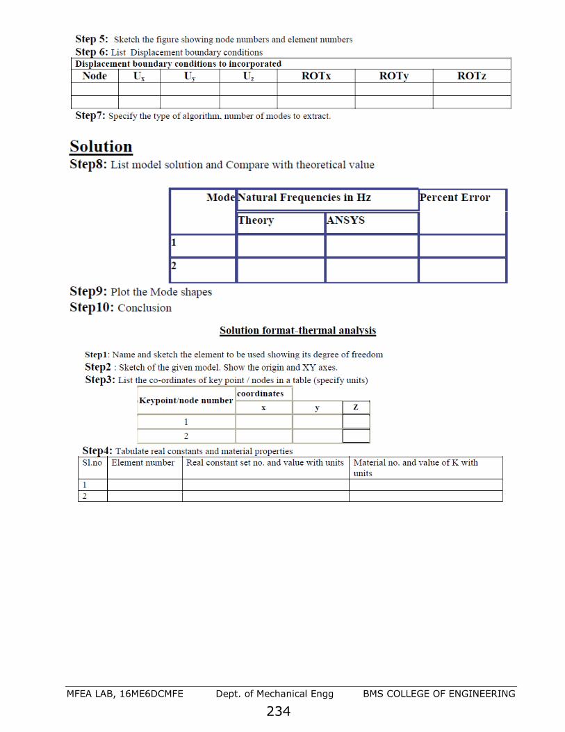
MFEA LAB, 16ME6DCMFE Dept. of Mechanical Engg BMS COLLEGE OF ENGINEERING
234

MFEA LAB, 16ME6DCMFE Dept. of Mechanical Engg BMS COLLEGE OF ENGINEERING
235

MFEA LAB, 16ME6DCMFE Dept. of Mechanical Engg BMS COLLEGE OF ENGINEERING
236
Acknowledgment
The department of Mechanical Engineering is deeply indebted and wish to
express sincere thanks to all the faculties who have contributed in the
preparation of this manual.