Modeling and discretization methods for the numerical simulation

of elastic stents ∗

Luka Grubisic† Matko Ljulj† Volker Mehrmann‡ Josip Tambaca†

January 22, 2019

Abstract

A new model description for the numerical simulation of elastic stents is proposed. Basedon the new formulation an inf-sup inequality for the finite element discretization is provedand the proof of the inf-sup inequality for the continuous problem is simplified. The newformulation also leads to faster simulation times despite an increased number of variables.The techniques also simplify the analysis and numerical solution of the evolution problemdescribing the movement of the stent under external forces. The results are illustrated vianumerical examples.

Keywords: elastic stent, mathematical modeling, numerical simulation, mixed finite elementformulation, stationary system, evolution equation,

AMS: 74S05, 74K10, 74K30, 74G15, 74H15, 65M15, 65M60

1 Introduction

In this paper we present a new model description for the dynamic and stationary simulationof stents. This new formulation is using constrained partial differential equations in mixedvariational weak form, which are based on a network structure consisting of one dimensionalcurved rods (struts). The new formulation will turn out to be particularly convenient for theanalysis of the partial differential equation, in particular in proving an inf-sup inequality whichdirectly transfers to a discrete inf-sup inequality in the discretized setting, so that from classicalresults of [3] the error estimates follow.

In the new formulation, the inextensibility and unshearability of the rod are expressed inthe weak formulation, but the continuity of the displacement and the modeling of infinitesimalrotations are modelled via constraints so that they do not have to be incorporated in the functionspaces as was done in the classical approach in [10]. This advantage of the new formulation comesalong with the introduction of new unknowns for the displacements and infinitesimal rotationsat vertices where different struts are connected and further unknowns for the contact couplesand contact forces at the end points of each strut. However, despite the introduction of manynew unknowns, the numerical solvers become more efficient for the large scale cases.

Stents, see Figure 1, are typically considered as a union of struts each of which is modeled bya 1D curved rod model, see [14, 15], and a set of junction conditions describing the connection

∗This work has been supported by Deutscher Akademischer Austauschdienst (DAAD) via Project Asymptoticand algebraic analysis of nonlinear eigenvalue problems in contact mechanics and electro magnetism. The thirdauthor is also supported by Einstein Foundation Berlin via Einstein Center ECMath Project: Model Reductionfor Nonlinear Parameter-Dependent Eigenvalue Problems in Photonic Crystals.†Department of Mathematics, Faculty of Science, University of Zagreb, Bijenicka 30, 10000 Zagreb,

luka,mljulj,tambaca@math.hr.§Institut fur Mathematik MA 4-5, TU Berlin, Str. des 17. Juni 136, D-10623 Berlin, FRG.

mehrmann@math.tu-berlin.de.

1

Figure 1: Example of an elastic stent (Cypher stent by Cordis Corporation)

of the struts, see [9]. The so-obtained model describes the three-dimensional behavior of stentsbut it has the complexity of a one-dimensional model. This model can be applied for anyelastic structure made of thin curved (or straight) rods. It was first formulated in [23] and thenreformulated in the weak form in [5]. The properties of the mixed formulation for the modelhave been analyzed in [10], numerical methods have been introduced, and error estimates havebeen derived in [12], but up to now error estimates for the contact forces, which are representedas Lagrange multipliers of the contact conditions, were missing. To derive these error estimatesis one of the main results of this paper.

To model the topology of the stent we use an undirected graph N = (V, E) consisting of aset V of nV vertices, which are the points where the middle lines of the rods meet and a set E ofnE edges that represent a 1D description of the curved rod. To be able to use a 1D curved rodmodel, we additionally need to prescribe the local geometry of the rod, i.e., the middle curveand the geometry of the cross-section as well as the material properties of the stent. These aregiven by

• the function Φi : [0, `i]→ R3 as natural parametrization of the middle line of the ith strutof length `i, represented by the edge ei ∈ E ,

• the shear modulus µi and the Young modulus Ei as parameters describing the material ofthe ith strut,

• as well as the width wi and the thickness ti of the rectangular cross-section of the ith strut.

Using these quantities, in the stationary case, see [23], the model for the ith strut ei ∈ E , isgiven by the following system of ordinary differential equations (in space)

0 = ∂spi + f i, (1.1)

0 = ∂sqi + ti × pi, (1.2)

0 = ∂sωi −Qi(Hi)−1(Qi)Tqi, (1.3)

0 = ∂sui + ti × ωi. (1.4)

where for the ith strut

• ui : [0, `i]→ R3 denotes the vector of displacements on the middle curve,

• ωi : [0, `i]→ R3 is the vector of infinitesimal rotations of the cross-section,

• qi is the contact moment and pi is the contact force,

• f i is the line density of the applied forces,

• Qi = [ti,ni, bi] is an orthogonal rotation matrix associated to the middle curve, withti = (Φi)′ being the unit tangent to the middle curve and ni, bi being vectors spanningthe normal plane to the middle curve, so that Qi represents the local basis at each pointof the middle curve,

2

• Hi = diag(µiKi, EiIin, EiIib) is a positive definite diagonal matrix, with the Young modulus

Ei, the shear modulus µi, Iin, Iib are the moments of inertia of the cross section and µiKi

is the torsional rigidity of the cross section.

Equations (1.1) and (1.2) represent equilibrium equations (for forces and moments), while (1.3)and (1.4) are constitutive relations. In particular, (1.4) describes the inextensibility and un-shearability of the struts, see [5] for more details.

In addition to equations (1.1)–(1.4), at each vertex of the stent we have a kinematic couplingcondition that u and ω are continuous and a dynamic coupling condition describing the balanceof contact forces p and contact moments q.

Denoting by J−j the set of all edges that leave the jth vertex, i.e., the local variable is equal

to 0 at vertex j and by J+j the set of all edges that enter the vertex, i.e., the local variable is

equal to `i for ith edge at the vertex j. With these notations we obtain the node conditions

ωi(0) = ωk(`k), i ∈ J−j , k ∈ J+j , j = 1, . . . , nV ,

ui(0) = uk(`k), i ∈ J−j , k ∈ J+j , j = 1, . . . , nV ,∑

i∈J+j

pi(`i)−∑i∈J−j

pi(0) = 0, j = 1, . . . , nV ,

∑i∈J+

j

qi(`i)−∑i∈J−j

qi(0) = 0, j = 1, . . . , nV .

(1.5)

Since this is a pure traction problem, we can integrate over s ∈ [0, `i] and specify a uniquesolution by requiring the two additional conditions∫

Nu :=

nV∑i=1

∫ `i

0ui ds = 0,

∫Nω :=

nV∑i=1

∫ `i

0ωi ds = 0, (1.6)

which means that the total displacement as well as the total infinitesimal rotation are zero.In the formulation of [10], the model is described on the collection of all displacements ui

and infinitesimal rotations ωi for all edges which are continuous on the whole stent. Thus, thetuples of unknowns in the problem uS = ((u1,ω1), . . . , (unE ,ωnE )) belong to the space

H1(N ;Rk) =

(y1, . . . ,ynE ) ∈

nE∏i=1

H1(0, `i;Rk) :

yi(0) = yk(`k), i ∈ J−j , k ∈ J+j , j = 1, . . . , nV

,

with H1(0, `i;Rk) being the Sobolov space of functions on [0, `i] whose derivatives up to thefirst derivative are square Lebesgue integrable. The formulation given in [10] is a mixed for-mulation with Lagrange multipliers appearing in the formulation due to the inextensibility andunshearability of the struts in the 1d curved rod model (1.4), and the two conditions on thetotal displacement and infinitesimal rotation (1.6). Under these conditions, in [10] an inf-supinequality was proved and the well-posedness of the problem was established. However, for thediscretized problem via the finite element method it would be necessary to also have a discreteinf-sup inequality to obtain an error estimate also for the Lagrange multipliers approximation.

We will show that the elastic energy is coercive in the space implementing inextensibility,unshearability, and continuity of displacement and infinitesimal rotation. Using the results of [3],we will show that the Lagrange multipliers are unique in both the old and the new formulationand for the discrete problem also in the new formulation. This is a considerable improvementcompared to the classical mixed formulation [12], where a proof of the discrete inf-sup inequalitywas not successful.

3

Let AI ∈ R3nV ,3nE denote the incidence matrix of the oriented graph (V, E) with threeconnected components, organized in the following way: a 3×3 submatrix at rows 3i−2, 3i−1, 3iand columns 3j − 2, 3j − 1, 3j is I3 if the edge j enters the vertex i, −I3 if it leaves the vertexi or 0 otherwise. Then the matrix A+

I is obtained from AI by setting all elements −1 to 0 andA−I is defined as AI = A+

I −A−I . Let us also introduce the projectors

PiE ∈ R3,3nE , Pj

V ∈ R3,3nV

on the coordinates 3i − 2, 3i − 1, 3i and 3j − 2, 3j − 1, 3j, respectively. We will also need thespaces

L2(N ;R3) =

nE⊗i=1

L2(0, `i;R3), L2Hr(N ;R3) =

nE⊗i=1

Hr(0, `i;R3), r ≥ 1

with associated norms

‖(y1, . . . ,ynE )‖L2(N ;R3) =

(nE∑i=1

‖yi‖2L2(0,`i;R3)

)1/2

,

‖(y1, . . . ,ynE )‖L2Hr (N ;R3) =

(nE∑i=1

‖yi‖2Hr(0,`i;R3)

)1/2

.

The norm corresponding to the last term for r = 1 is also used as the norm for H1(N ;R6). Fora function y = (y1, . . . ,ynE ) ∈ L2

H1(N ;R3) by y′ we denote (∂sy1, . . . , ∂sy

nE ) ∈ L2(N ;R3).The results that we prove for the continuous model in Section 3 hold for general geometries,

while the results for the discrete approximation in Section 4 are proved only for stent geometrieswith straight struts.

The paper is organized as follows. In Section 2 we present the new formulation of the stentmodel. In Section 3 we analyze the new model and give a proof of the inf-sup inequality forthe weak formulation of the continuous infinite dimensional model and in Section 4 we analyzethe discrete model that is obtained after finite element discretization and show a correspondinginf-sup inequality. Finally in Section 5 we study the dynamical system of the stent movementunder excitation forces. We analyze the properties and present numerical simulation results.

2 New formulation of the model

In this section we reformulate the stent model in a way that enables the proof of a discreteinf-sup inequality and then, using classical results, appropriate error estimates follow. For this,we treat all unknowns in the problem explicitly and do not encode them in the function spacesor the weak formulation. In this way not only the inextensibility and unshearability of the rodis expressed in the weak formulation, but the continuity of the displacement and infinitesimalrotation is reflected in the function space of the mixed formulation in H1(N ;R6). This leadsto the introduction of new unknowns, displacements and infinitesimal rotations at vertices, andfurther, the contact moments and contact forces at the ends of each strut.

Since u and ω are continuous over the whole stent, we introduce as extra variables thedisplacements and infinitesimal rotations at the vertices U i,Ωi, i = 1, . . . , nV , and then formthe vectors

U = [U1, . . . ,UnV ]T , Ω = [Ω1, . . . ,ΩnV ]T .

Then the kinematic coupling at the vertex j leads to the conditions

ui(`i) = U j , i ∈ J+j , ui(0) = U j , i ∈ J−j ,

ωi(`i) = Ωj , i ∈ J+j , ωi(0) = Ωj , i ∈ J−j .

(2.1)

4

To express the dynamic coupling conditions, we introduce the contact moments and forces atthe ends of the struts,

Qi+ = qi(`i), Qi

− = qi(0), P i+ = pi(`i), P i

− = pi(0), i = 1, . . . , nE (2.2)

and defineP± = (P 1

±, . . . ,PnE± ), Q± = (Q1

±, . . . ,QnE± ).

Then the dynamic coupling conditions at the vertex j can be expressed as∑i∈J+

j

P i+ −

∑i∈J−j

P i− = 0,

∑i∈J+

j

Qi+ −

∑i∈J−j

Qi− = 0, j = 1, . . . , nE . (2.3)

Equations (1.1)–(1.4), (2.1), (2.2), (2.3), and (1.6) together constitute the stent problem in ournew formulation for which we now derive in detail the weak formulation.

We multiply the ith equation of (1.1) by vi ∈ H1(0, `i;R3) and that of (1.2) by wi ∈H1(0, `i;R3), add them, integrate over s ∈ [0, `i], and sum the equations over i. This yields

0 =

nE∑i=1

∫ `i

0∂sp

i · vi + f i · vi + ∂sqi ·wi + ti × pi ·wi ds.

After partial integration we obtain

0 =

nE∑i=1

∫ `i

0

(−pi · ∂svi + f i · vi − qi · ∂swi−ti ×wi · pi

)ds+ pi · vi

∣∣`i0

+ qi ·wi∣∣`i0,

i.e.,

nE∑i=1

∫ `i

0

(−pi · (∂svi + ti ×wi)− qi · ∂swi

)ds

+ P i+ · vi(`i)− P i

− · vi(0) +Qi+ ·wi(`i)−Qi

− ·wi(0) = −nE∑i=1

∫ `i

0f i · vi ds.

(2.4)

In a similar way we multiply (1.3) by ξi ∈ L2(0, `i;R3) and (1.4) by θi ∈ L2(0, `i;R3) integrateover s ∈ [0, `i] and sum all equations to obtain

0 =

nE∑i=1

∫ `i

0−∂sωi · ξi + Qi(Hi)−1(Qi)Tqi · ξi − (∂su

i + ti × ωi) · θi ds. (2.5)

We also multiply the equations in (2.3) for the jth vertex by V j and W j from R3, respectively,and sum the equations over j which gives

nV∑j=1

∑i∈J+

j

P i+ −

∑i∈J−j

P i−

· V j +

nV∑j=1

∑i∈J+

j

Qi+ −

∑i∈J−j

Qi−

·W j = 0.

Since∑

i∈J+jP i

+ = PjVA

+I P+ and

∑i∈J−j

P i− = Pj

VA−I P−, this equation can be written as

nV∑j=1

PjV(A+I P+ −A−I P−

)· V j +

nV∑j=1

PjV(A+IQ+ −A−IQ−

)·W j = 0,

and, therefore, (A+I P+ −A−I P−

)· V +

(A+IQ+ −A−IQ−

)·W = 0 (2.6)

5

for all V = [V 1, . . . ,V nV ]T , W = [W 1, . . . ,W nV ]T ∈ R3nV .Multiplying the equations for the displacements in (2.1) by Θi

+ and Θi−, we obtain

ui(`i) ·Θi+ = U j ·Θi

+, i ∈ J+j , ui(0) ·Θi

− = U j ·Θi−, i ∈ J−j .

Since PiE(A

+I )TU = U j for i ∈ J+

j , for Θ± = [Θ1±, . . . ,Θ

nE± ]T we have

nE∑i=1

ui(`i) ·Θi+ = (A+

I )TU ·Θ+,

nE∑i=1

ui(0) ·Θi− = (A−I )TU ·Θ−, Θ+,Θ− ∈ R3nE ,

and similarly, for the rotations, using the notation Ξ± = [Ξ1±, . . . ,Ξ

nE± ]T , we get

nE∑i=1

ωi(`i) ·Ξi+ = (A+

I )TΩ ·Ξ+,

nE∑i=1

ωi(0) ·Ξi− = (A−I )TΩ ·Ξ−, Ξ+,Ξ− ∈ R3nE .

Thus, we have

nE∑i=1

(ui(`i) ·Θi+ − ui(0) ·Θi

−)− (A+I )TU ·Θ+ + (A−I )TU ·Θ− = 0, Θ+,Θ− ∈ R3nE , (2.7)

for the displacements and

nE∑i=1

(ωi(`i) ·Ξi+ − ωi(0) ·Ξi

−)− (A+I )TΩ ·Ξ+ + (A−I )TΩ ·Ξ− = 0, Ξ+,Ξ− ∈ R3nE (2.8)

for the rotations. We multiply the equations (1.6) by α and β, respectively, and summing up,we obtain

α ·∫Nu+ β ·

∫Nω = 0, α,β ∈ R3. (2.9)

Subtracting (2.6) from (2.4), we obtain

nE∑i=1

∫ `i

0

(−pi · (∂svi + ti ×wi)− qi · ∂swi

)ds

+

nE∑i=1

(P i+ · vi(`i)− P i

− · vi(0)) +

nE∑i=1

(Qi+ ·wi(`i)−Qi

− ·wi(0))

−(A+I P+ −A−I P−

)· V −

(A+IQ+ −A−IQ−

)·W = −

nE∑i=1

∫ `i

0f i · vi ds,

vi,wi ∈ H1(0, `i;R3), i = 1, . . . , nE , V ,W ∈ R3nV .

(2.10)

We then add (2.7) and (2.8) to (2.5) and obtain

nE∑i=1

∫ `i

0Qi(Hi)−1(Qi)Tqi · ξi − (∂su

i + ti × ωi) · θi − ∂sωi · ξi ds

+

nE∑i=1

(ui(`i) ·Θi+ − ui(0) ·Θi

−) +

nE∑i=1

(ωi(`i) ·Ξi+ − ωi(0) ·Ξi

−)

− ((A+I )TU ·Θ+ − (A−I )TU ·Θ−)− ((A+

I )TΩ ·Ξ+ − (A−I )TΩ ·Ξ−) = 0,

ξi,θi ∈ L2(0, `i;R3), i = 1, . . . , nE , Θ±,Ξ± ∈ R3nE .

(2.11)

In [10] and [12] the mixed formulation of the stent model was presented using the spaceH1(N ;R3) for the displacement vector u and the infinitesimal rotation vector ω. The space

6

L2(N ;R3) × R3 × R3 for the Lagrange multipliers p,α,β, and the continuity conditions fordisplacements and infinitesimal rotations were inherently built into the space H1(N ;R3). Wenow relax these conditions and consider them as additional equations in the problem and enlargethe space of unknowns by adding further Lagrange multipliers. The resulting function spacesare given by

V = L2(N ;R3)× L2(N ;R3)× R3nE × R3nE × R3nE × R3nE × R3 × R3,

M = L2H1(N ;R3)× L2

H1(N ;R3)× R3nV × R3nV .

To simplify the notation for the elements of these spaces we introduce

Σ := (q,p,P+,P−,Q+,Q−,α,β) ∈ V, φ := (u,ω,U ,Ω) ∈M

for the unknowns in the problem and

Γ := (ξ,θ,Θ+,Θ−,Ξ+,Ξ−,γ, δ) ∈ V, ψ := (v,w,V ,W ) ∈M

for the associated test functions.In this notation, the bilinear forms and the linear functionals that appear in the above

calculations are given by

a : V × V → R, b : V ×M → R, f : M → R,

a(Σ,Γ) :=

nE∑i=1

∫ `i

0Qi(Hi)−1(Qi)Tqi · ξi ds,

b(Σ,ψ) :=

nE∑i=1

∫ `i

0

(−pi · (∂svi + ti ×wi)− qi · ∂swi

)ds

+

nE∑i=1

(P i+ · vi(`i)− P i

− · vi(0)) +

nE∑i=1

(Qi+ ·wi(`i)−Qi

− ·wi(0))

−(A+I P+ −A−I P−

)· V −

(A+IQ+ −A−IQ−

)·W +α ·

∫Nv + β ·

∫Nw,

f(ψ) := −nE∑i=1

∫ `i

0f i · vi ds.

Then the variational formulation (2.10), (2.11) and (2.9) can be expressed as follows.Determine Σ ∈ V and φ ∈M such that

a(Σ,Γ) + b(Γ,φ) = 0, Γ ∈ V,b(Σ,ψ) = f(ψ), ψ ∈M.

(2.12)

In this way we have obtained that the solution of the stent problem as formulated in (1.1)–(1.6)satisfies (2.12) and conversely that any solution of (2.12) satisfies (1.1)–(1.6).

In this section we have reformulated the mathematical formulation of the stent model byincluding the continuity conditions at the nodes as extra equations and by adding further La-grange multipliers. In the next sections, we will use this formulation to obtain a discrete inf-supinequality and to present a simpler proof of the continuous inf-sup inequality.

3 Properties of the continuous model

In this section we consider the properties of the continuous operator equation (2.12). For theoperator B : V →M ′ defined by

M ′〈BΣ,ψ〉M = b(Σ,ψ), ψ ∈M

7

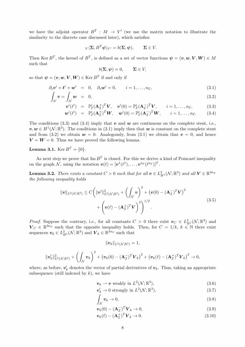
we have the adjoint operator BT : M → V ′ (we use the matrix notation to illustrate thesimilarity to the discrete case discussed later), which satisfies

V 〈Σ, BTψ〉V ′ = b(Σ,ψ), Σ ∈ V.

Then KerBT , the kernel of BT , is defined as a set of vector functions ψ = (v,w,V ,W ) ∈ Msuch that

b(Σ,ψ) = 0, Σ ∈ V,so that ψ = (v,w,V ,W ) ∈ KerBT if and only if

∂svi + ti ×wi = 0, ∂sw

i = 0, i = 1, . . . , nE , (3.1)∫Nv =

∫Nw = 0, (3.2)

vi(`i) = PiE(A

+I )TV , vi(0) = Pi

E(A−I )TV , i = 1, . . . , nE , (3.3)

wi(`i) = PiE(A

+I )TW , wi(0) = Pi

E(A−I )TW , i = 1, . . . , nE . (3.4)

The conditions (3.3) and (3.4) imply that v and w are continuous on the complete stent, i.e.,v,w ∈ H1(N ;R3). The conditions in (3.1) imply then that w is constant on the complete stentand from (3.2) we obtain w = 0. Analogously, from (3.1) we obtain that v = 0, and henceV = W = 0. Thus we have proved the following lemma.

Lemma 3.1. KerBT = 0.

As next step we prove that ImBT is closed. For this we derive a kind of Poincare inequalityon the graph N , using the notation v(`) = [v1(`1), . . . ,vnE (`nE )]T .

Lemma 3.2. There exists a constant C > 0 such that for all v ∈ L2H1(N ;R3) and all V ∈ R3nV

the following inequality holds

‖v‖L2(N ;R3) ≤ C(‖v′‖2L2(N ;R3) +

(∫Nv

)2

+(v(0)− (A−I )TV

)2+

(v(`)− (A+

I )TV

)2)1/2

.

(3.5)

Proof. Suppose the contrary, i.e., for all constants C > 0 there exist vC ∈ L2H1(N ;R3) and

V C ∈ R3nV such that the opposite inequality holds. Then, for C = 1/k, k ∈ N there existsequences vk ∈ L2

H1(N ;R3) and V k ∈ R3nV such that

‖vk‖L2(N ;R3) = 1,

‖v′k‖2L2(N ;R3) +

(∫Nvk

)2

+(vk(0)− (A−I )TV k

)2+(vk(`)− (A+

I )TV k

)2 → 0,

where, as before, v′k denotes the vector of partial derivatives of vk. Thus, taking an appropriatesubsequence (still indexed by k), we have

vk v weakly in L2(N ;R3), (3.6)

v′k → 0 strongly in L2(N ;R3), (3.7)∫Nvk → 0, (3.8)

vk(0)− (A−I )TV k → 0, (3.9)

vk(`)− (A+I )TV k → 0. (3.10)

8

It follows that on each strut we have

vik vi weakly in L2(0, `i;R3), ∂svik → 0 strongly in L2(0, `i;R3), i = 1, . . . , nE ,

so that vi is constant on the ith strut and

vik vi weakly in H1(0, `i;R3).

By the Trace Theorem; see e.g. [7, Section 5.5, Theorem 1] we have then

vik(0)→ vi, vik(`i)→ vi.

Using (3.9) and (3.10), we have

PiE(A

−I )TV k → vi, Pi

E(A+I )TV k → vi, i = 1, . . . , nE . (3.11)

Since in every block row of size 3 the matrices (A−I )T and (A+I )T have exactly one identity

matrix of size 3 we have that V k is convergent as well. We denote the limit by V , and havethat its values are given by vi suitably organized. Therefore, since AI = A+

I −A−I , subtractingthe sequences in (3.11) we obtain that

ATIV = 0.

Since the rank of ATI is equal to 3nV−3, the kernel of AT

I is of dimension 3 by the Rank–NullityTheorem, [1]. We easily inspect that Ker AT

I is spanned by the vectors

(e1, e1, . . . , e1), (e2, e2, . . . , e2), (e3, e3, . . . , e3).

Thus we obtain that all vi are equal. Since 0 =∫N v =

∑nEi=1 `

ivi, we obtain that vi = 0 andhence V = 0, which also implies that v = 0. Thus, since

vik(x) = vik(0) +

∫ x

0∂sv

ik(s) ds,

(vik)k tends to 0 strongly in L2(0, `i;R3) for all i = 1, . . . , nE , which is in contradiction to theunit norm assumption of the sequence, i.e., ‖vk‖L2(N ;R3) = 1.

Lemma 3.3. ImBT is closed.

Proof. Consider a convergent sequence in ImBT , i.e., a sequence of the form

∂svik + ti ×wi

k → pi, ∂swik → qi, strongly in L2(0, `i;R3) i = 1, . . . , nE ,∫

Nvk → α,

∫Nwk → β,

vik(`i)− PiE(A

+I )TV k → P i

+, vik(0)− PiE(A

−I )TV k → P i

−,

wik(`i)− Pi

E(A+I )TW k → Qi

+, wik(0)− Pi

E(A−I )TW k → Qi

−.

(3.12)

Then applying the inequality (3.5) to the sequenceswk = (w1k, . . . ,w

nEk ) andW k = (W 1

k, . . . ,WnEk )

implies that wk is bounded in L2(N ,R3). Therefore, wik is bounded in H1(0, `i;R3) and hence

there exists a subsequence and a function wi ∈ H1(0, `i;R3) such that

wikl wi weakly in H1(0, `i;R3), i = 1, . . . , nE .

We collect the limits in w = (w1, . . . ,wnE ) and, using again the Trace Theorem, we obtain that

qi = ∂swi, −Pi

E(A+I )TW kl → Qi

+ −wi(`i), −PiE(A

−I )TW kl → Qi

− −wi(0),

9

for i = 1, . . . , nE and

β =

∫Nw.

Since in each block row of dimension 3 the matrices A±I have exactly one identity matrix, weobtain that W kl converges to W which satisfies

−PiE(A

+I )TW = Qi

+ −wi(`i), −PiE(A

−I )TW = Qi

− −wi(0), i = 1, . . . , nE .

By inequality (3.5), there is a unique function w that satisfies the associated homogeneoussystem

∂swi = 0, i = 1, . . . , nE ,

∫Nw = 0, v(0)− (A−I )TV = v(`)− (A+

I )TV = 0.

Therefore, w is unique and thus the whole sequences (wk)k and (W k)k are convergent. Applica-tion of Lemma 3.2 to wk−w and W k−W implies that wk → w strongly in L2

H1(N ;R3). Oncewe have this convergence we apply it to the term ti×wi

k and by the same reasoning identify alllimits related to vk and V k. We obtain vk → v strongly in L2

H1(N ;R3) and V k → V in R3nV

and that

∂svi + ti ×wi = pi, vi(`i)− Pi

E(A+I )TV = P i

+, vi(0)− Pi

E(A−I )TV = P i

−, α =

∫Nu.

Thus Σ = (q,p,P+,P−,Q+,Q−,α,β) belongs to ImBT , and hence ImBT is closed.

As a direct consequence of Lemmas 3.1, 3.3, and [4, Proposition 1.2, page 39], we obtain thefollowing corollary.

Corollary 3.4 (Continuous inf-sup inequality). Consider the variational formulation of thestent model (2.12). Then there exists a constant kc > 0 such that

infψ∈M

supΣ∈V

b(Σ,ψ)

‖Σ‖V ‖ψ‖M≥ kc.

As our next result we will prove the KerB ellipticity of the form a, i.e., that there existca > 0 such that

a(Σ,Σ) ≥ ca‖Σ‖2V , Σ ∈ KerB.

To obtain this result, we need to restrict the class of networks we consider.

Lemma 3.5. Let the stent geometry be such that∑i∈J+

jith edge is straight

αiti −

∑i∈J−

jith edge is straight

αiti = 0, j = 1, . . . , nV

implies that αi = 0 for all straight edges i. Then the bilinear form a from the variationalformulation (2.12) is KerB elliptic.

Proof. The space KerB is given by the set of Σ = (q,p,P+,P−,Q+,Q−,α,β) ∈ V such that

b(Σ,ψ) = 0, ψ ∈M.

Thus, from the definition of the form b one has that for all ψ = (v,w,V ,W ) ∈MnE∑i=1

∫ `i

0

(−pi · (∂svi + ti ×wi)− qi · ∂swi

)ds

+

nE∑i=1

(P i+ · vi(`i)− P i

− · vi(0)) +

nE∑i=1

(Qi+ ·wi(`i)−Qi

− ·wi(0))

−(A+I P+ −A−I P−

)· V −

(A+IQ+ −A−IQ−

)·W +α ·

∫Nv + β ·

∫Nw = 0.

(3.13)

10

Since V and W in RnV are arbitrary, we obtain

A+I P+ −A−I P− = A+

IQ+ −A−IQ− = 0, (3.14)

which is equivalent to (2.3). These conditions mean that at each vertex the sum of the contactforces as well as the sum of the contact moments are zero. Then, for γ ∈ R3, we insert vi = γ,wi = 0, W = V = 0 as test functions in (3.13) and obtain

nE∑i=1

(P i+ − P i

−) · γ +α ·(

nE∑i=1

`i

)γ = 0.

Since from (3.14)nE∑i=1

(P i+ − P i

−) =

nE∑i=1

PiE(A

+I P+ −A−I P−) = 0,

we obtain that α = 0. Now, for fixed i we insert vi ∈ C1([0, `i];R3) with compact support in

〈0, `i〉 in (3.13) and obtain∫ `i

0 pi · ∂svi = 0. This implies that pi is a constant on each strut.

Inserting a single vi ∈ C1([0, `i];R3) in (3.13), we obtain that

−pi ·∫ `i

0∂sv

i ds+ P i+ · vi(`i)− P i

− · vi(0) = 0 (3.15)

and thus pi = P i+ = P i

−.Similarly, for γ ∈ R3 we insert wi = γ for all i in (3.13) and obtain

−nE∑i=1

∫ `i

0pi × ti · γ ds+

nE∑i=1

(Qi+ −Qi

−) · γ + β ·(

nE∑i=1

`i

)γ = 0.

As in the case of contact forces we have∑nE

i=1(Qi+ −Qi

−) = 0. For the first term we argue asfollows

nE∑i=1

∫ `i

0pi × ti ds =

nE∑i=1

pi × (Φi(`i)−Φi(0)) =

nV∑j=1

(∑i∈J+

j

P i+ −

∑i∈J−j

P i−)× Vj = 0,

again by (3.14), where Vj denotes the jth vertex. Thus we conclude that β = 0. What is leftfrom (3.13) are the equations for all i ∈ 1, . . . , nE and all wi ∈ H1(0, `i) given by

−∫ `i

0pi × ti ·wi ds−

∫ `i

0qi · ∂swi ds+Qi

+ ·wi(`i)−Qi− ·wi(0) = 0. (3.16)

Defining qi = qi − pi × (Φi(s)−Φi(0)) and inserting this form in (3.16), we obtain

−∫ `i

0pi × ti ·wi ds−

∫ `i

0qi · ∂swi ds−

∫ `i

0pi × (Φi(s)−Φi(0)) · ∂swi ds

+Qi+ ·wi(`i)−Qi

− ·wi(0) = 0.

After partial integration in the third term we obtain

−∫ `i

0qi · ∂swi ds+ (Qi

+ − pi × (Φi(`i)−Φi(0))) ·wi(`i)−Qi− ·wi(0) = 0. (3.17)

As in the case of contact forces, see (3.15), this implies that the qi are constants and that

qi = Qi+ − pi × (Φi(`i)−Φi(0)) = Qi

−, i = 1, . . . , nE .

11

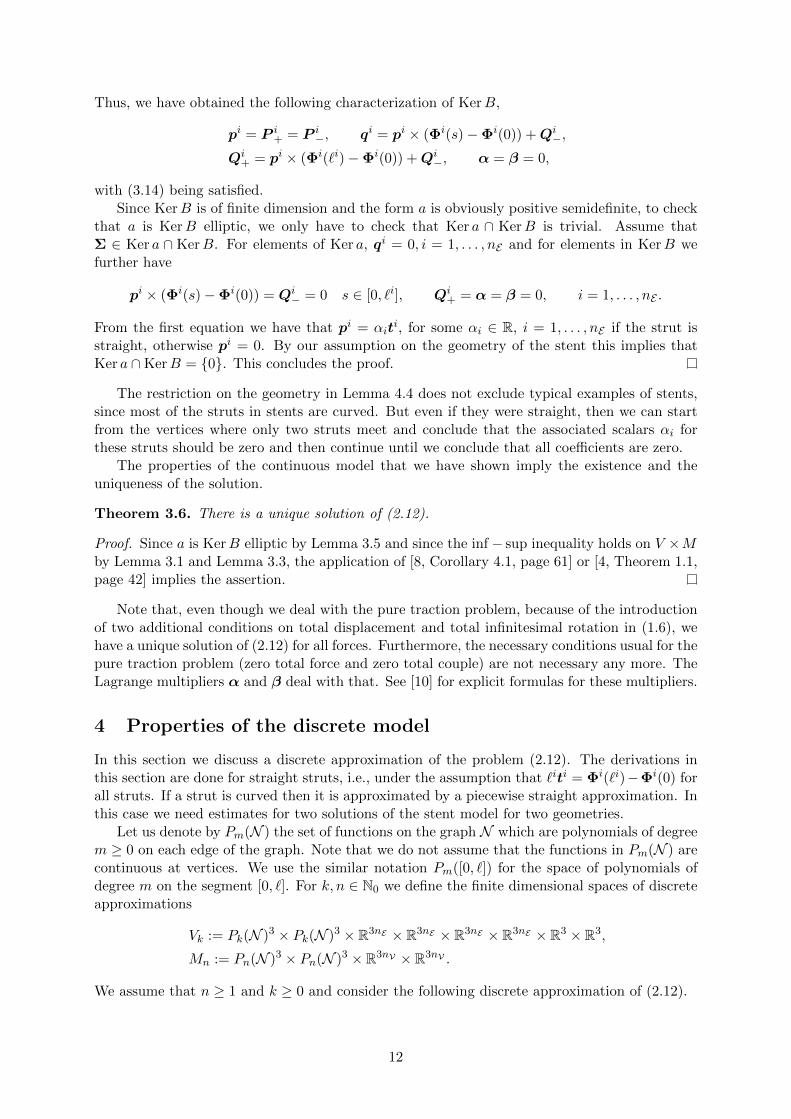
Thus, we have obtained the following characterization of KerB,

pi = P i+ = P i

−, qi = pi × (Φi(s)−Φi(0)) +Qi−,

Qi+ = pi × (Φi(`i)−Φi(0)) +Qi

−, α = β = 0,

with (3.14) being satisfied.Since KerB is of finite dimension and the form a is obviously positive semidefinite, to check

that a is KerB elliptic, we only have to check that Ker a ∩ KerB is trivial. Assume thatΣ ∈ Ker a ∩ KerB. For elements of Ker a, qi = 0, i = 1, . . . , nE and for elements in KerB wefurther have

pi × (Φi(s)−Φi(0)) = Qi− = 0 s ∈ [0, `i], Qi

+ = α = β = 0, i = 1, . . . , nE .

From the first equation we have that pi = αiti, for some αi ∈ R, i = 1, . . . , nE if the strut is

straight, otherwise pi = 0. By our assumption on the geometry of the stent this implies thatKer a ∩KerB = 0. This concludes the proof.

The restriction on the geometry in Lemma 4.4 does not exclude typical examples of stents,since most of the struts in stents are curved. But even if they were straight, then we can startfrom the vertices where only two struts meet and conclude that the associated scalars αi forthese struts should be zero and then continue until we conclude that all coefficients are zero.

The properties of the continuous model that we have shown imply the existence and theuniqueness of the solution.

Theorem 3.6. There is a unique solution of (2.12).

Proof. Since a is KerB elliptic by Lemma 3.5 and since the inf − sup inequality holds on V ×Mby Lemma 3.1 and Lemma 3.3, the application of [8, Corollary 4.1, page 61] or [4, Theorem 1.1,page 42] implies the assertion.

Note that, even though we deal with the pure traction problem, because of the introductionof two additional conditions on total displacement and total infinitesimal rotation in (1.6), wehave a unique solution of (2.12) for all forces. Furthermore, the necessary conditions usual for thepure traction problem (zero total force and zero total couple) are not necessary any more. TheLagrange multipliers α and β deal with that. See [10] for explicit formulas for these multipliers.

4 Properties of the discrete model

In this section we discuss a discrete approximation of the problem (2.12). The derivations inthis section are done for straight struts, i.e., under the assumption that `iti = Φi(`i)−Φi(0) forall struts. If a strut is curved then it is approximated by a piecewise straight approximation. Inthis case we need estimates for two solutions of the stent model for two geometries.

Let us denote by Pm(N ) the set of functions on the graph N which are polynomials of degreem ≥ 0 on each edge of the graph. Note that we do not assume that the functions in Pm(N ) arecontinuous at vertices. We use the similar notation Pm([0, `]) for the space of polynomials ofdegree m on the segment [0, `]. For k, n ∈ N0 we define the finite dimensional spaces of discreteapproximations

Vk := Pk(N )3 × Pk(N )3 × R3nE × R3nE × R3nE × R3nE × R3 × R3,

Mn := Pn(N )3 × Pn(N )3 × R3nV × R3nV .

We assume that n ≥ 1 and k ≥ 0 and consider the following discrete approximation of (2.12).

12

Determine Σ ∈ Vk and φ ∈Mn such that

a(Σ,Γ) + b(Γ,φ) = 0, Γ ∈ Vk,b(Σ,ψ) = f(ψ), ψ ∈Mn.

(4.1)

The form b on Vk ×Mn defines the operator Bh : Vk →M ′n, where M ′n denotes the dual of Mn.In general, however, KerBh is not a subset of KerB. However, we will show that if n − 1 ≥ kthen it is a subset and thus applying Lemma 3.5 gives the following result.

Lemma 4.1. Consider the discrete problem (4.1) and let n− 1 ≥ k. Then the bilinear form ais KerBh elliptic.

Proof. As in the continuous case, the elements Σ = (q,p,P+,P−,Q+,Q−,α,β) of KerBh

satisfy (3.14) and by the same arguments it follows that α = 0. For fixed i and a test functionvi ∈ Pn([0, `i]) we obtain the equation

−∫ `i

0pi · ∂svi ds+ P i

+ · vi(`i)− P i− · vi(0) = 0.

For constant vi = γ ∈ R3, we obtain P i+ = P i

− and, inserting pi = pi + P i− implies

−∫ `i

0pi · ∂svi ds = 0, vi ∈ Pn([0, `i]).

Since n ≥ k + 1, the function pi is zero and hence pi = P i+ = P i

−.For vi = 0, i = 1, . . . , nE and V = W = 0 in (3.13) we obtain

nE∑i=1

∫ `i

0−pi · ti ×wi − qi · ∂swi ds+

nE∑i=1

(Qi+ ·wi(`i)−Qi

− ·wi(0)) + β ·∫Nw = 0. (4.2)

Inserting wi = γ ∈ R3, i = 1, . . . , nE , we obtain

nE∑i=1

−γ ·∫ `i

0pi × ti ds+

nE∑i=1

(Qi+ −Qi

−) · γ + β ·(

nE∑i=1

`i

)γ = 0.

As in the proof of Lemma 3.5, we obtain that β = 0, and thus we are left with the equation

−pi× ti ·∫ `i

0wi ds−

∫ `i

0qi ·∂swi ds+Qi

+ ·wi(`i)−Qi− ·wi(0) = 0, wi ∈ Pn([0, `i]). (4.3)

For k ≥ 1, we insert qi = qi + spi × ti into this equation and obtain

−pi × ti ·∫ `i

0wi ds−

∫ `i

0qi · ∂swi ds− pi × ti ·

∫ `i

0s∂sw

i ds+Qi+ ·wi(`i)−Qi

− ·wi(0) = 0.

After partial integration in the third term we obtain

−∫ `i

0qi · ∂swi ds+ (Qi

+ − `ipi × ti) ·wi(`i)−Qi− ·wi(0) = 0.

Since constant functions are contained in Vk, for wi = γ we obtain Qi+ = Qi

− + `ipi × ti. Then

setting qi = ˜q +Qi−, we obtain∫ `i

0

˜qi · ∂swi ds = 0, wi ∈ Pn([0, `i]).

13

As before, since n− 1 ≥ k, this implies that ˜q = 0, and hence qi = Qi− + spi × ti.

For k = 0, qi is constant, so from (4.3) we obtain

−pi × ti ·∫ `i

0wi ds− qi · (wi(`i)−wi(0)) +Qi

+ ·wi(`i)−Qi− ·wi(0) = 0.

This implies thatpi × ti = 0, qi = Qi

+ = Qi−

and we have obtained the characterization of KerBh given by (q,p,P+,P−,Q+,Q−,α,β) thatsatisfy (3.14) and

pi = P i+ = P i

−, α = β = 0, qi = Qi− + spi × ti, Qi

+ = Qi− + `ipi × ti.

Additionally, if k = 0, then pi × ti = 0. Thus, KerBh = KerB ∩ Vk ⊆ KerB and hence a iselliptic on KerBh by Lemma 3.5.

Lemma 4.2. Consider the discrete problem (4.1) and let k ≥ n− 1. Then KerBTh = 0.

Proof. KerBTh is defined as a set of ψ = (v,w,V ,W ) ∈Mn such that

b(Σ,ψ) = 0, Σ = (q,p,P+,P−,Q+,Q−,α,β) ∈ Vk.

Thus, ψ = (v,w,V ,W ) ∈ KerBTh if and only if

nE∑i=1

∫ `i

0−pi · (∂svi + ti ×wi)− qi · ∂swi ds

+

nE∑i=1

(P i+ · vi(`i)− P i

− · vi(0)) +

nE∑i=1

(Qi+ ·wi(`i)−Qi

− ·wi(0))

−(A+I P+ −A−I P−

)· V −

(A+IQ+ −A−IQ−

)·W +α ·

∫Nv + β ·

∫Nw = 0

for all Σ ∈ Vk. This is equivalent to

nE∑i=1

∫ `i

0

(−pi · (∂svi + ti ×wi)− qi · ∂swi

)ds = 0,pi, qi ∈ Pk([0, `i]), (4.4)

i = 1, . . . , nE , (4.5)∫Nv =

∫Nw = 0, (4.6)

vi(`i) = PiE(A

+I )TV , vi(0) = Pi

E(A−I )TV , i = 1, . . . , nE , (4.7)

wi(`i) = PiE(A

+I )TW , wi(0) = Pi

E(A−I )TW , i = 1, . . . , nE . (4.8)

Since k ≥ n − 1, from (4.4) for a test function qi we obtain that wi is constant for each strut.The continuity of the infinitesimal rotations at the vertices follows from (4.8). This implies thatwi = const and then (4.6) implies that wi = 0, i.e., wi = 0 for all i = 1, . . . , nE and W = 0.Analogous arguments using (4.7) imply that vi = 0 and V = 0 as well.

Let n = k + 1, so that both Lemma 4.1 and Lemma 4.2 apply. Since we are in the finitedimensional case, clearly ImBh is closed. Proposition 1.2, page 39 in [4] then implies thatImBh = (KerBT

h )0 and then by Lemma 4.2 it follows that ImBh = M ′n. Furthermore, byLemma 4.1, the bilinear form a is KerBh elliptic. Then, by the classical theory for finitedimensional approximations of mixed formulations, e.g. Proposition 2.1 in [4], we obtain thefollowing existence and uniqueness result for the discretized problem.

14

Theorem 4.3. Let n = k + 1. Then problem (4.1) has a unique solution.

Applying the classical results then also we obtain the discrete inf-sup inequality.

Corollary 4.4 (Discrete inf-sup inequality). If n = k + 1, then there exists a constant kd > 0such that

infψ∈Mn

supΣ∈Vk

b(Σ,ψ)

‖Σ‖Vk‖ψ‖Mn

≥ kd.

Proof. By Corollary 3.4, the continuous inf-sup inequality holds. By Lemma 3.1 and Lemma 4.2we have KerBT

h = KerBT = 0. Thus Proposition 2.2, page 53 in [4] implies that the as-sumptions of Proposition 2.8, page 58 in [4] are fulfilled and we obtain the discrete inf-supinequality.

Remark 4.1. Note that the constant kd from Corollary 4.4 depends on the subspaces Vk andMn.

Using Theorem 2.1, page 60 in [4], the discrete inf-sup inequality in Corollary 4.4 andLemma 4.1, i.e., the coercivity of the form a on KerBh, we obtain error estimates also in thediscrete problem. Introducing analogous notation as in the continuous case,

Σh := (qh,ph,P h+,P

h−,Q

h+,Q

h−,α

h,βh) ∈ Vk, φh := (uh,ωh,Uh,Ωh) ∈Mn

for the unknowns in the problem and

Γh := (ξh,θh,Θh+,Θ

h−,Ξ

h+,Ξ

h−,γ

h, δh) ∈ Vk, ψh := (vh,wh,V h,W h) ∈Mn

for the test functions we have the following theorem.

Theorem 4.5. Let n = k + 1 and let (Σ,φ) ∈ V × M be the solution of (2.12) and let(Σh,φh) ∈ Vk ×Mn be the solution of (4.1). Then

‖Σ−Σh‖V + ‖φ− φh‖M ≤ c(

infΓh∈Vk

‖Σ− Γh‖V + infψh∈Mn

‖φ−ψh‖M).

Remark 4.2. The construction of finite elements, as presented, is directly related to the strutswhich are described by their prescribed length. To increase the accuracy we can increase thepolynomial degree, assuming that the geometry has been described without error. On the otherhand, we can change the topology of the stent by adding new points on existing struts (and thusnot changing the geometry of the stent) in the original definition of the graph N = (V, E). Inthis way we obtain a refined model with transmission conditions of continuity of displacements,rotations, contact moments and forces at new points. Since at each new vertex only two strutsmeet, these transmission conditions are the same coupling conditions (kinematical and dynam-ical) as for all vertices of the stent. Thus, the resulting weak formulations as in [5] or [10] arethe same for both networks, the original one and the one with added vertices.

The error estimate in Theorem 4.5 can be employed in the finite element method usinginterpolation estimates in L2 and H1. Note that in contrast to the numerical method in [12],due to the availability of the discrete inf-sup inequality in the new formulation, we obtain theerror estimate for all variables, including the contact forces. It is a classical result, see e.g. [6],that for a function ϕ ∈ Hr(0, `) and its polynomial Lagrange interpolant Πmϕ of degree m onehas the estimate

‖ϕ−Πmϕ‖L2(0,`) ≤ C`min r,m+1‖ϕ(min r,m+1)‖L2(0,`), ϕ ∈ Hr(0, `),

‖ϕ−Πmϕ‖H1(0,`) ≤ C`min r−1,m‖ϕ(min r,m+1)‖L2(0,`), ϕ ∈ Hr(0, `).(4.9)

With h := max`i, i = 1, . . . , nE, then combining (4.9) with Theorem 4.5, we obtain thefollowing error estimate for the finite element method.

15

Theorem 4.6. Let n = k + 1, r ≥ 0, r ∈ N, and let f ∈ L2Hr(N ;R3). Let (Σ,φ) ∈ V ×M be

the solution of (2.12) and (Σh,φh) ∈ Vk ×Mn the solution of (4.1). Then

‖Σ−Σh‖V + ‖φ− φh‖M ≤ chmin r+1,k+1‖f‖L2Hr.

Proof. The error of the finite element approximation is estimated by the error of the interpolationoperator. Thus we get

‖Σ−Σh‖V + ‖φ− φh‖M ≤ c(‖Σ−ΠkΣ‖V + ‖φ−Πnφ‖M

).

Since in this section the struts are assumed to be straight for f ∈ L2Hr(N ;R3), from the differ-

ential equations we obtain that

p ∈ L2Hr+1(N ;R3), q ∈ L2

Hr+2(N ;R3), ω ∈ L2Hr+3(N ;R3), u ∈ L2

Hr+4(N ;R3).

Thus, we obtain the estimate

‖Σ−Σh‖V + ‖φ− φh‖M≤ c(hmin r+1,k+1‖(q,p)(min r+1,k+1)‖L2(N ;R6)

+ hmin r+2,n‖(u,ω)(min r+3,n+1)‖L2(N ;R6)

)≤ c(hmin r+1,k+1‖f‖L2

Hmin r,k+ hmin r+2,n‖f‖L2

Hmin r,n−2

)≤ chmin r+1,k+1‖f‖L2

Hr.

Note that for k = 1 and n = 2 and r ≥ 1 we obtain quadratic convergence in the H1 normfor the displacements and infinitesimal rotations. This is in accordance with the convergencerate obtained in [12] for the classical formulation.

Having obtained error estimates for the continuous and discrete problem, in the next sub-section, we consider the properties of the resulting linear system.

4.1 Block structure of the discretization matrix

In the sequel we assume that n = k+ 1. Using the same structure as in the continuous problem,the discrete problem is given by a linear system Kx = F , where

K =

[A BT

B 0

], F =

[0F 2

]with a square matrix A of size 3(2k+6)nE+6 and a rectangular matrix B of size (3(2k+4)nE+6nV)× (3(k + 6)nE + 6). Having in mind the evolution problem that we will study in the nextsection, we partition these matrices further as

A =

[A11 0

0 0

], B =

[0 B32

B41 B42

], (4.10)

where A11 is a square matrix of size 3(k+1)nE , B32 is a matrix of size 3(k+2)nE×(3(k+5)nE+6),B41 is of size (3(k+2)nE+6nV)×3(k+1)nE and B42 is of size (3(k+2)nE+6nV)×(3(k+5)nE+6)associated with the following variables,

dim \ unknown q (p,P+,P−,Q+,Q−,α,β) u (ω,U ,Ω) F

3(k + 1)nE A11 0 0 BT41 0

3(k + 5)nE + 6 0 0 BT32 BT

42 0

3(k + 2)nE 0 B32 0 0 F 3

3(k + 4)nE + 6nV B41 B42 0 0 0

16

Figure 2: Design of the Palmaz like stent used in simulations

or in more detail,

q p P+ P− Q+ Q− α β u ω U Ω dimension

ξ ⋆ 0 ⋆ 3(k + 1)nEθ ⋆ ⋆ 3(k + 1)nET+ ⋆ −(A+

I )T 3nE

T− ⋆ (A−I )

T 3nEΞ+ ⋆ −(A+

I )T 3nE

Ξ− ⋆ (A−I )

T 3nEγ ⋆ 3

δ ⋆ 3

v 0 ⋆ ⋆ ⋆ ⋆ 0 3(k + 2)nEω ⋆ ⋆ ⋆ ⋆ ⋆ 3(k + 2)nEV −A+

I A−I 3nV

W −A+I A−

I 3nV

4.2 Numerical results

To illustrate our theoretical analysis we test the implementation of the numerical scheme in thenew formulation for a Palmaz type stent as in Figure 2. The radius of the stent is 1.5mm andthe overall length is 1.68cm. There are 144 vertices in the associated graph with 276 straightedges. All vertices except the boundary ones are junctions of four edges. The cross-sections areassumed to be square with the side length 0.1mm. The material of the stent is stainless steelwith Young modulus E = 2.1 · 1011 and Poisson ratio ν = 0.26506. To this structure we applythe forcing normal to the axis of the of stent, i.e. of the form

f(x) = f(x1)x2e2 + x3e3√

x22 + x23, x = (x1, x2, x3) ∈ R3, (4.11)

where x1 is the axis of the cylinder. As a consequence, the deformation will also posess someradial symmetry. The problem is a pure traction problem and the applied forces satisfy thenecessary condition. The non-uniqueness of the solution in the problem is fixed using theLagrange multipliers α and β.

The solution for the forcing function

f(x1) =10

105(x1 − `/2)2 + 1, (4.12)

is presented in Figure 3; here ` is the length of the stent. On the left the solution is projected tothe (x1, x2)–plane, while on the right it is shown from the different perspective. For the forcingfunction

f(x1) = 103(x1 − `/2)2e3 (4.13)

17

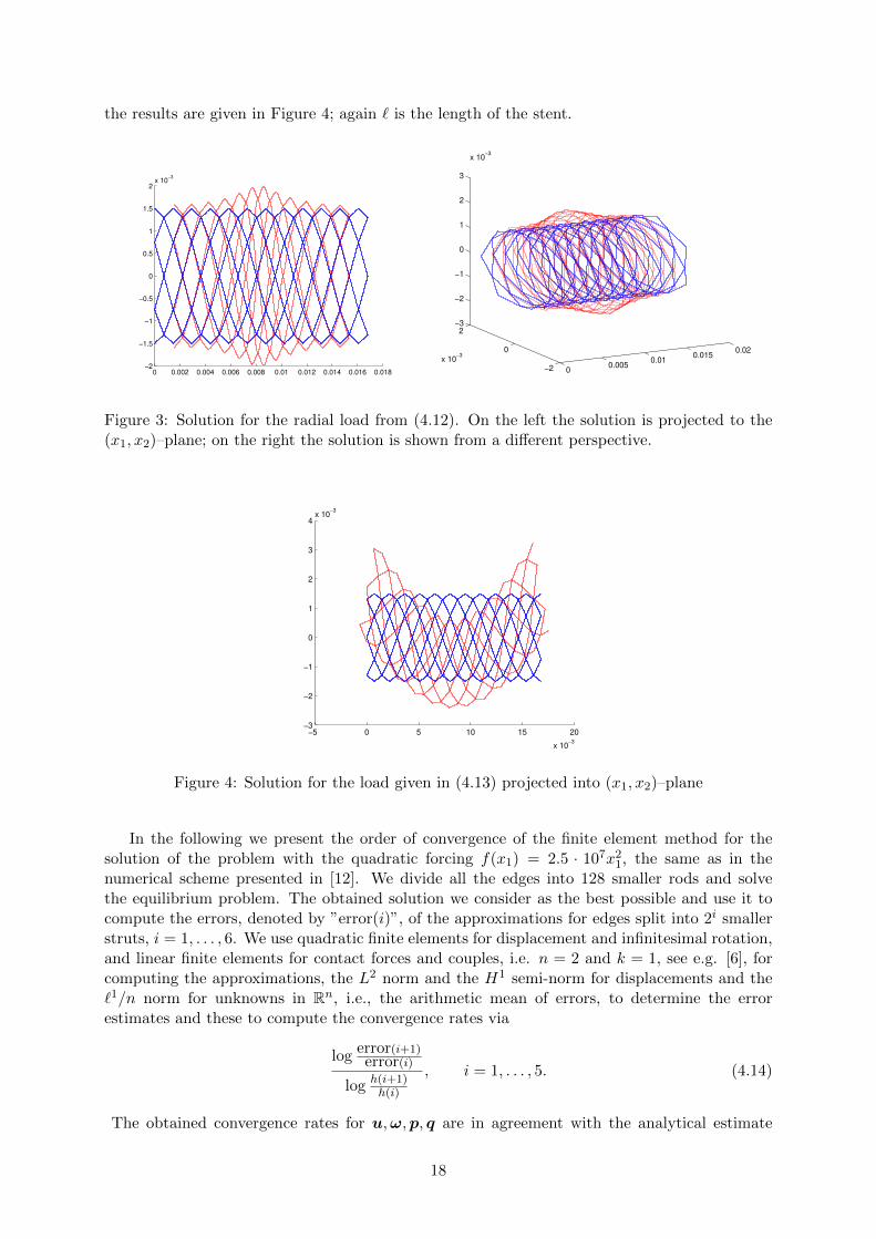
the results are given in Figure 4; again ` is the length of the stent.

0 0.002 0.004 0.006 0.008 0.01 0.012 0.014 0.016 0.018−2

−1.5

−1

−0.5

0

0.5

1

1.5

2x 10

−3

00.005

0.010.015

0.02

−2

0

2

x 10−3

−3

−2

−1

0

1

2

3

x 10−3

Figure 3: Solution for the radial load from (4.12). On the left the solution is projected to the(x1, x2)–plane; on the right the solution is shown from a different perspective.

−5 0 5 10 15 20

x 10−3

−3

−2

−1

0

1

2

3

4x 10

−3

Figure 4: Solution for the load given in (4.13) projected into (x1, x2)–plane

In the following we present the order of convergence of the finite element method for thesolution of the problem with the quadratic forcing f(x1) = 2.5 · 107x21, the same as in thenumerical scheme presented in [12]. We divide all the edges into 128 smaller rods and solvethe equilibrium problem. The obtained solution we consider as the best possible and use it tocompute the errors, denoted by ”error(i)”, of the approximations for edges split into 2i smallerstruts, i = 1, . . . , 6. We use quadratic finite elements for displacement and infinitesimal rotation,and linear finite elements for contact forces and couples, i.e. n = 2 and k = 1, see e.g. [6], forcomputing the approximations, the L2 norm and the H1 semi-norm for displacements and the`1/n norm for unknowns in Rn, i.e., the arithmetic mean of errors, to determine the errorestimates and these to compute the convergence rates via

log error(i+1)error(i)

log h(i+1)h(i)

, i = 1, . . . , 5. (4.14)

The obtained convergence rates for u,ω,p, q are in agreement with the analytical estimate

18

1 1.5 2 2.5 3 3.5 4 4.5 51.5

2

2.5

3

3.5

4

4.5

5

p

P+

P−

Figure 5: Rate of convergence (4.14) for the L2 norm of the contact force p and `1 norm ofP+,P−

1 1.5 2 2.5 3 3.5 4 4.5 51.5

2

2.5

3

3.5

4

4.5

5

u

u in H1

U

Figure 6: Rate of convergence (4.14) for the H1 seminorm and L2 norm of the displacement uand `1 norm of U

from Theorem 4.6 for k = 1 and n = 2. In Figure 5 the convergence rates for p,P+ and P− aredisplayed, while in Figure 6 the convergence rates for the u (L2 norm and H1 semi-norm) andU are plotted. Additionally we present the errors of the remaining unknowns in Table 1.

To compare the numerical scheme for the new formulation with that for the old formulationin [12] in Table 2, we present the obtained matrix sizes and the computing times (computingtimes are determined using difference of ”toc” and ”tic” functions in MATLAB 2010b.) for thecomputation on a personal computer with 16GB RAM, 64bit Windows and with INTEL R©Corei3-7100 CPU@3.90FHz.

The difference between the solution for the displacement u, infinitesimal rotation ω and thecontact force p (the only quantities calculated in the old numerical scheme from [12]) for thesame splitting of edges is at least four digits smaller than the error of the approximation, i.e.

19

splitting q Q+ Q− ω Ω

2 1.8127e-5 3.1945266e-8 3.2871209e-8 8.52118e-4 3.3700235e-54 0.4532e-5 0.1995776e-8 0.2024711e-8 1.06516e-4 0.2116646e-58 0.1133e-5 0.0124898e-8 0.0125802e-8 0.13314e-4 0.0132275e-5

16 0.0283e-5 0.0007811e-8 0.0007839e-8 0.01664e-4 0.0008260e-532 0.0070e-5 0.0000486e-8 0.0000487e-8 0.00208e-4 0.0000514e-564 0.0017e-5 0.0000028e-8 0.0000028e-8 0.00025e-4 0.0000030e-5

Table 1: Errors for different splitting of edges (L2 errors for q and ω).

new formulation old formulation

splitting # comp. time in s size of matrix comp. time in s size of matrix

8 22 105198 2 3895816 47 211182 42 7870232 108 423150 152 15819064 288 847086 629 317166128 903 1694958 4183 635118

Table 2: Computing times and matrix sizes for the old and new numerical scheme

we obtain the same order of approximation for the same mesh. Further, the size of the matrixfor the new numerics is 2.7 times larger. However, the computing times for the new approachare smaller when splitting the edges in 32 or more rods.

5 Dynamic modeling of elastic stents

In the previous sections we have considered the static problem for the stent, but for the analysis,in particular, to study the movement of the stent under the permanent excitation through theheartbeat, in this section we formulate and analyze the evolution model of the stents.

5.1 Formulation of the space-continuous dynamic model

In order to formulate the dynamic model we start from the evolution equation of curved rodsfrom [22] and add in the model (1.1)–(1.4) the inertial term to the equilibrium equation (1.1),which changes to

ρAuitt = ∂sp

i + f i,

where A is the area of the cross section and ρ is volume density of mass. In the weak formulationthis implies that the term

−nE∑i=1

∫ `i

0ρAui

tt · vi ds

should be added to the left hand side of (2.4) and (2.10). Using the notation of Section 2 andintroducing the bilinear form

c : M ×M → R, c(φ,ψ) =

nE∑i=1

∫ `i

0ρAui · vi ds,

we can formulate the evolution problem of elastic stents as follows:

20

Determine Σ and Γ such that

a(Σ,Γ) + b(Γ,φ) = 0, Γ ∈ V,

− d2

dt2c(φ,ψ) + b(Σ,ψ) = f(ψ), ψ ∈M.

(5.1)

5.2 Analysis of the space-discrete model

The dynamical system (5.2) is a finite dimensional linear differential-algebraic equation of secondorder, with a nonsingular (but indefinite) stiffness matrix K, and a positive semidefinite butsingular E.

The associated discrete dynamical problem is given by

−Ez(t) + Kz(t) = F (t), (5.2)

where the matrix K and the right hand side F are as in the static case, E has the followingstructure partitioned as K

dim \ unknown q (p,P+,P−,Q+,Q−,α,β) u (ω,U ,Ω)

3(k + 1)nE 0 0 0 0

3(k + 5)nE + 6 0 0 0 0

3(k + 2)nE 0 0 M 0

3(k + 4)nE + 6nV 0 0 0 0

,

and z(t) is the vector of coefficient functions in the finite element basis.The particular block structure of the DAE allows to analyze the properties of the system,

which are characterized by the spectral properties of the matrix polynomial −λ2E + K.

Lemma 5.1. Consider the DAE (5.2) and the associated pair of matrices (E,K). Then thereexists a nonsingular matrix V with the property that

E = VTEV =

0

00

M0

, V−1z =

z1z2z3z4z5

,

K = VTKV =

0 0 0 0 BT

51

0 A22 0 BT42 0

0 0 A33 0 0

0 B42 0 0 0

B51 0 0 0 0

, VTF =

000

F 4

0

,

where A33 = AT33, B42, and B51 are invertible, and F 4 = F 3.

Proof. The proof follows by a sequence of congruence transformations, starting from the originalblock structure

E =

0

0M

0

, K =

A11 0 0 BT

41

0 0 BT32 BT

42

0 B32 0 0B41 B42 0 0

,by first compressing [

0 B32

B41 B42

]21

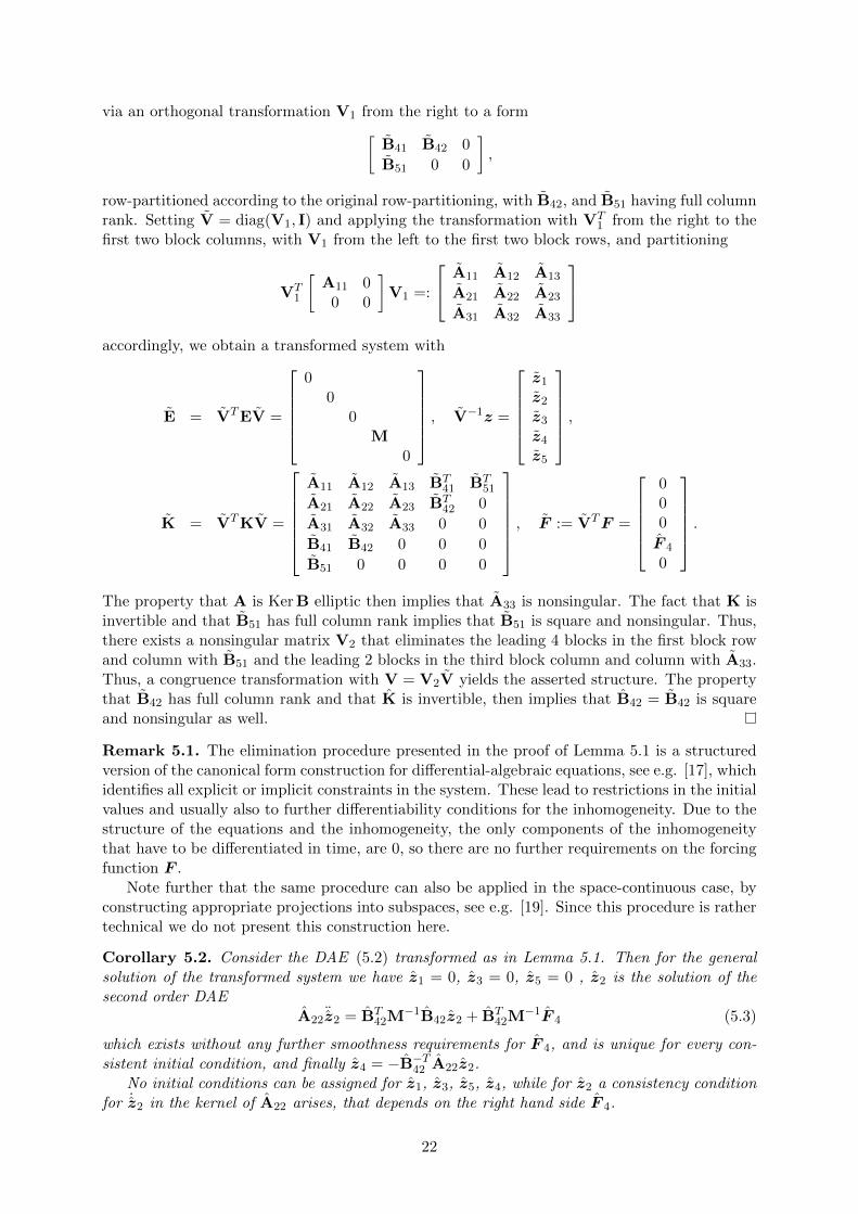
via an orthogonal transformation V1 from the right to a form[B41 B42 0

B51 0 0

],

row-partitioned according to the original row-partitioning, with B42, and B51 having full columnrank. Setting V = diag(V1, I) and applying the transformation with VT

1 from the right to thefirst two block columns, with V1 from the left to the first two block rows, and partitioning

VT1

[A11 0

0 0

]V1 =:

A11 A12 A13

A21 A22 A23

A31 A32 A33

accordingly, we obtain a transformed system with

E = VTEV =

0

00

M0

, V−1z =

z1z2z3z4z5

,

K = VTKV =

A11 A12 A13 BT

41 BT51

A21 A22 A23 BT42 0

A31 A32 A33 0 0

B41 B42 0 0 0

B51 0 0 0 0

, F := VTF =

000

F 4

0

.

The property that A is Ker B elliptic then implies that A33 is nonsingular. The fact that K isinvertible and that B51 has full column rank implies that B51 is square and nonsingular. Thus,there exists a nonsingular matrix V2 that eliminates the leading 4 blocks in the first block rowand column with B51 and the leading 2 blocks in the third block column and column with A33.Thus, a congruence transformation with V = V2V yields the asserted structure. The propertythat B42 has full column rank and that K is invertible, then implies that B42 = B42 is squareand nonsingular as well.

Remark 5.1. The elimination procedure presented in the proof of Lemma 5.1 is a structuredversion of the canonical form construction for differential-algebraic equations, see e.g. [17], whichidentifies all explicit or implicit constraints in the system. These lead to restrictions in the initialvalues and usually also to further differentiability conditions for the inhomogeneity. Due to thestructure of the equations and the inhomogeneity, the only components of the inhomogeneitythat have to be differentiated in time, are 0, so there are no further requirements on the forcingfunction F .

Note further that the same procedure can also be applied in the space-continuous case, byconstructing appropriate projections into subspaces, see e.g. [19]. Since this procedure is rathertechnical we do not present this construction here.

Corollary 5.2. Consider the DAE (5.2) transformed as in Lemma 5.1. Then for the generalsolution of the transformed system we have z1 = 0, z3 = 0, z5 = 0 , z2 is the solution of thesecond order DAE

A22¨z2 = BT

42M−1B42z2 + BT

42M−1F 4 (5.3)

which exists without any further smoothness requirements for F 4, and is unique for every con-sistent initial condition, and finally z4 = −B−T42 A22z2.

No initial conditions can be assigned for z1, z3, z5, z4, while for z2 a consistency conditionfor ˙z2 in the kernel of A22 arises, that depends on the right hand side F 4.

22

Proof. This follows directly from the transformed equations. The equations (5.3) form a socalled index-one DAE (see [17]), since BT

42M−1B42 is positive definite and thus, in particular

invertible in the kernel of A22. Projecting into this kernel gives an algebraic equation which hasto hold for the initial condition associated with ˙z2, while for the remaining components of z2an initial value can can be chosen arbitrarily.

Remark 5.2. The operator pencil associated to the system (5.1) can be studied using thegeneral theory from [21]. Note that the form e((Σ,φ), (Γ,ψ)) = c(φ,ψ), (Σ,φ), (Γ,ψ) ∈V ⊗M is bounded and symmetric and the form k((Σ,φ), (Γ,ψ)) = a(Σ,Γ) + b(Γ,φ) + b(Σ,ψ),(Σ,φ), (Γ,ψ) ∈ V ⊗M is closed, symmetric and semi-bounded from below, see [11]. The form edefines, in the sense of Kato [16], the bounded, semidefinite and self-adjoint operator E, whereasthe form k defines the self-adjoint semibounded from below operator K. The operator K canbe represented as the formal product K = L∗JL, where L is a closed operator with a boundedinverse such that the domains of L and k are equal and J is the so called fundamental symmetry(a bounded self adjoint operator such that J2 = J). Subsequently it can be shown — using thespecial structure of E — that the operator function T (z) = −z2E + K, where E = L−∗EL−1

and K = J , is Fredholm operator valued. Furthermore, the operators E and K are boundedHermitian operators and the resolvent set of T contains zero by Theorem 3.6. By the resultsof [21, Section 1], the pencil T has finite semi-simple eigenvalues of finite multiplicity. Theconstruction of an oblique projection onto the reducing subspace associated to the eigenvalueinfinity can be done in a similar way as in Lemma 5.1. The construction is decidedly moretechnical and we leave it to a subsequent paper where we will discuss more general second ordersystems (e.g. those involving a damping term).

5.3 Numerical results

In this subsection we present some numerical results obtained for the evolution problem. Thetime discretization is done using the implicit mid point rule [13] (of convergence order 2) appliedto the first order formulation of the system. At each time step a linear system for the matrix−E+0.25∆t2K is solved using backslash in MATLAB. The computations are performed on a personalcomputer with 16GB RAM, 64bit Windows and with INTEL R©Core i3-7100 CPU@3.90FHz. Thepresented computing times are determined using the difference of ”toc” and ”tic” functions inMATLAB 2010b. All simulations are carried out for the following set of parameters:

• elasticity coefficients: µ = E = 1 Pa,

• thickness of the stent struts: 0.0001 m,

• load: radial, as given in (4.11), where

f(x, t) = F( π

0.003(x− cvawe(t− t0))

)(5.4)

with

F (y) =

5 · 10−8 cos(y), if |y| < 0.00150, else

, cvawe = 0.0075, t0 = 0.5.

In other words, f is given as traveling wave determined by the function F , where the factorcvawe denotes the speed of the wave and the term t0 asserts the condition f(x, ·) = 0.

• mass density ρ = 2000 kg/m3,

• total time T = 12s.

In Figure 7 the solutions of the problem for the force f in (5.4) at the time-points t ∈1, 2, 3, 4, 5, 6s is plotted.

23

0 5 10 15 20

x 10−3

−1.5

−1

−0.5

0

0.5

1

1.5

x 10−3

0 5 10 15 20

x 10−3

−1.5

−1

−0.5

0

0.5

1

1.5

x 10−3

0 5 10 15 20

x 10−3

−1.5

−1

−0.5

0

0.5

1

1.5

x 10−3

0 5 10 15 20

x 10−3

−1.5

−1

−0.5

0

0.5

1

1.5

x 10−3

0 5 10 15 20

x 10−3

−1.5

−1

−0.5

0

0.5

1

1.5

x 10−3

0 5 10 15 20

x 10−3

−1.5

−1

−0.5

0

0.5

1

1.5

x 10−3

Figure 7: Solution of the problem projected to the (x1, x2)–plane for loads given in (5.4) and attimes t = 1s, 2s, 3s, 4s, 5s, and 6s.

In the sequel we compare the computing times of two different approaches. In the firstapproach we use the MATLAB backslash function to solve the system obtained at every timestep. In the second, we first perform the LDLT decomposition of the matrix −E + 0.25∆t2K,since it is the same in all iterations and then in the time integration we use the obtained LDLT

decomposition to solve the system.In the Table 5.3 the computing times for two different calculations with different space

discretizations are presented. In the first column the number of splits in the longest edge (strut)in the stent is displayed. The second column displays the associated number of degrees offreedom. The remaining columns present the computing times. The results indicate that theuse of the factorization LDLT obviously pays off. Here the time step is equal to 2−4.

In Table 5.3 we compare computing times for different time step sizes with the same finaltime T . The total time approximately doubles when lowering ∆t which is natural, since the

24

no LDL using LDLT

# splits size of matrix time (s) time for precomputation (s) time for iterations (s)

20 12462 476 1.34 11021 25710 554 1.70 20322 52206 793 4.62 39223 105198 1338 23.71 855

Table 3: Computing times for several space discretizations without and with LDLT precompu-tation.

number of time steps doubles. However, it is interesting to note that the time for the solutionwith LDLT reduces when reducing ∆t. Here every strut is split in 4 smaller struts.

no LDL using LDLT

∆t time (s) time for precomputation (s) time for iterations (s)

2−3 277 3.66 2022−4 554 1.77 3922−5 1120 1.52 8082−6 2332 1.39 1717

Table 4: Computing times for several values of ∆t without and with LDLT precomputation.

We have also computed the errors in the solutions. For the same time step we computedthe errors for different number of strut splits. The errors are presented in Table 5.3. They arecalculated by comparing the solution with the solution for 24 strut splits. All errors are presentedin the L2(0, T ;L2(N )) norm. In Table 5.3 the errors are given for different ∆t and for fixed

h−1 error

20 0.04111079676079421 0.01534850177895222 0.00352472245804823 0.000224774470258

Table 5: Relative L2(0, T ;L2(N )) errors for different space meshes.

space mesh. The errors are computed with respect to ∆t = 2−7 and the same L2(0, T ;L2(N ))norm.

∆t error

2−3 0.0383702787649792−4 0.0230141490227352−5 0.0120512251643782−6 0.003154110021893

Table 6: Relative L2(0, T ;L2(N )) errors for different time steps.

Movies of the dynamic behavior of the stent are presented in the video Appendix.

25

6 Conclusion

We have presented a new model description for the numerical simulation of elastic stents, whichexplicitly displays all constraints. Based on the new formulation an inf-sup inequality for thefinite element discretization is shown and, furthermore, a simplified proof of the inf-sup inequalityfor the space continuous problem is presented. Despite an increased number of degrees offreedom, the new formulation leads to faster simulation time. The presented techniques arealso used to simplify the analysis and numerical solution of the evolution problem describingthe movement of the stent under external forces. Numerical examples illustrate the theoreticalresults and show the effectiveness of the new modeling approach.

References

[1] R. B. Bapat, Graphs and matrices, Springer, London; Hindustan Book Agency, NewDelhi, 2014.

[2] C. Beattie, V. Mehrmann, H. Xu, and H. Zwart, Linear port-Hamiltonian descrip-tor systems, Math. Control Signals Systems, 30 (2018), 17 (27 pages).

[3] D. Boffi, F. Brezzi, and M. Fortin, Mixed Finite Element Methods and Applications,Springer, Heidelberg, 2013.

[4] F. Brezzi and M. Fortin, Mixed and Hybrid Finite Element Methods, Springer, NewYork, 1991.

[5] S. Canic and J. Tambaca, Cardiovascular stents as PDE nets: 1D vs. 3D, IMA J. Appl.Math., 77 (2012), pp. 748–770.

[6] P.G. Ciarlet, The Finite Element Method for Elliptic Problems, Society for Industrialand Applied Mathematics (SIAM), Philadelphia, 2002.

[7] L.C. Evans, Partial Differential Equations, American Mathematical Society, Providence,1998.

[8] V. Girault and P.-A. Raviart, Finite Element Methods for Navier-Stokes Equations.Theory and Algorithms, Springer, Berlin, 1986.

[9] G. Griso, Asymptotic behavior of structures made of curved rods, Anal. Appl. (Singap.),6 (2008), pp. 11–22.

[10] L. Grubisic, J. Ivekovic, J. Tambaca, and B. Zugec, Mixed formulation of the one-dimensional equilibrium model for elastic stents, Rad Hrvat. Akad. Znan. Umjet. Mat.Znan., 21(532) (2017), pp. 219–240.

[11] L. Grubisic, V. Kostrykin, K.A. Makarov, and K. Veselic, Representation theo-rems for indefinite quadratic forms revisited, Mathematika, 59 (2013), pp. 169–189.

[12] L. Grubisic and J. Tambaca, Direct solution method for the equilibrium problem forelastic stents, Numer. Lin. Algebra Appl., to appear, 2019.

[13] E. Hairer and G. Wanner, Solving Ordinary Differential Equations II: Stiff andDifferential-Algebraic Problems, 2nd revised edition. Springer Verlag, Heidelberg, 1996.

[14] M. Jurak and J. Tambaca, Derivation and justification of a curved rod model, Math.Models Methods Appl. Sci., 9 (1999), pp. 991–1014.

26

[15] M. Jurak and J. Tambaca, Linear curved rod model. General curve, Math. ModelsMethods Appl. Sci., 11 (2001), 1237–1252.

[16] T. Kato, Perturbation Theory for Linear Operators, Springer Science & Business Media,New York, 2013.

[17] P. Kunkel and V. Mehrmann, Differential–Algebraic Equations. Analysis and Numer-ical Solution, European Mathematical Society (EMS), Zurich, 2006.

[18] P. Kunkel, V. Mehrmann, and L. Scholz, Self-adjoint differential-algebraic equa-tions, Math. Control Signals Systems, 26 (2014), 47–76.

[19] , R. Lamour, R. Marz, and C. Tischendorf, Differential-Algebraic Equations: AProjector Based Analysis, Springer Science & Business Media, Heidelberg, 2013.

[20] D.S. Mackey, N. Mackey, C. Mehl, and V. Mehrmann, Structured polynomialeigenvalue problems: good vibrations from good linearizations, SIAM J. Matrix Anal. Appl.,28 (2006), pp. 1029–1051.

[21] R. Mennicken and M. Moller, Non-Self-Adjoint Boundary Eigenvalue Problems,North-Holland Publishing Co., Amsterdam, 2003.

[22] J. Tambaca, Justification of the dynamic model of curved rods, Asympt. Anal., 31 (2002),43–68.

[23] J. Tambaca, M. Kosor, S. Canic, and D. Paniagua, Mathematical modeling ofvascular stents, SIAM J. Appl. Math., 70 (2010), pp. 1922–1952.

27