TKK Dissertations 95Espoo 2007

MODELING AND DETECTION OF HIGH IMPEDANCE ARCING FAULT IN MEDIUM VOLTAGE NETWORKSDoctoral Dissertation

Helsinki University of TechnologyDepartment of Electrical and Communications EngineeringPower Systems and High Voltage Engineering

Nagy Ibrahim Elkalashy

TKK Dissertations 95Espoo 2007

Dissertation for the degree of Doctor of Science in Technology to be presented with due permission of the Department of Electrical and Communications Engineering for public examination and debate in Auditorium S4 at Helsinki University of Technology (Espoo, Finland) on the 26th of November, 2007, at 12 noon.

Helsinki University of TechnologyDepartment of Electrical and Communications EngineeringPower Systems and High Voltage Engineering

Teknillinen korkeakouluSähkö- ja tietoliikennetekniikan osastoSähköverkot ja suurjännitetekniikka

Nagy Ibrahim Elkalashy

MODELING AND DETECTION OF HIGH IMPEDANCE ARCING FAULT IN MEDIUM VOLTAGE NETWORKSDoctoral Dissertation

Distribution:Helsinki University of TechnologyDepartment of Electrical and Communications EngineeringPower Systems and High Voltage EngineeringP.O. Box 3000FI - 02015 TKKFINLANDURL: http://powersystems.tkk.fi/eng/Tel. +358-9-451 5049Fax +358-9-451 5012E-mail: nagy.elkalashy@tkk.fi

© 2007 Nagy Ibrahim Elkalashy

ISBN 978-951-22-9014-7ISBN 978-951-22-9015-4 (PDF)ISSN 1795-2239ISSN 1795-4584 (PDF) URL: http://lib.tkk.fi/Diss/2007/isbn9789512290154/

TKK-DISS-2363

Multiprint OyEspoo 2007

HELSINKI UNIVERSITY OF TECHNOLOGY

P. O. BOX 1000, FI-02015 TKK

http://www.tkk.fi

ABSTRACT OF DOCTORAL DISSERTATION

Author Nagy Ibrahim Elkalashy

Name of the dissertation

Modeling and Detection of High Impedance Arcing Fault in Medium Voltage Networks

Date of manuscript 18.09.2007 Date of the dissertation 26.11.2007

Monograph Article dissertation (summary + original articles)

Department Electrical and Communications Engineering Laboratory Power Systems and High Voltage Engineering Field of research Electrical Power Systems Opponents Professor Mansour Abdel-Rahman Dr. Seppo Hänninen Supervisors Professor Matti Lehtonen, Helsinki University of Technology, Finland Professor Mohamed A. Izzularab, Minoufiya University, Egypt Professor Abdel-Maksoud I. Taalab, Minoufiya University, Egypt Ass. Professor Hatem A. Darwish, Minoufiya University, Egypt

Abstract:

In this dissertation, a universal arc representation using the Electromagnetic Transient Program (EMTP) is first developed. It is accomplished based on the bilateral interaction between EMTP network and Transient Analysis Control System (TACS) field. This arc modeling procedure is used as a useful guide to present a new model for high impedance arcing faults due to leaning trees. At the Power Systems and High Voltage Laboratory, Helsinki University of Technology (TKK), Finland, experiments have been performed to measure the fault characteristics due to leaning trees and therefore to verify the proposed model. Towards investigating detection facilities of this fault type, the fault model is incorporated at different locations in 20 kV Medium Voltage (MV) networks using the ATPdraw program, which is a graphical interface utilized to simplify the ATP/EMTP processing. Then, phase quantities and residual components are taken at different measuring nodes in the simulated networks. It is revealed that the main feature of this fault type that can enhance its detection is the periodicity of electromagnetic transients created by repetitions of the arc-reignition after each current zero-crossing. This feature is obtained considering different earthing concepts. Different detection techniques are proposed based on Discrete Wavelet Transform (DWT). The absolute sum of the wavelet coefficients in the respective frequency band is investigated for the detection purposes while several selectivity functions are proposed for the first time. The selectivity functions are presented using Logic Functions, fundamental current components and transient power directionalities. Test cases provide evidence of the efficacy of the proposed techniques. This dissertation is written in a form of the article dissertation. Its core depends on both of a summary and six original publications.

Keywords: Arc Models, Earth Faults, High Impedance Arcing Faults and Fault Detection.

ISBN 978-951-22-9014-7 ISSN 1795-2239

ISBN 978-951-22-9015-4 (PDF) ISSN 1795-4584 (PDF)

ISBN (others) Number of pages xiv + 160 p.

Publisher: Helsinki University of Technology, Power Systems and High Voltage Engineering

Print distribution: Power Systems and High Voltage Engineering

The dissertation can be read at http://lib.tkk.fi/Diss/isbn9789512290154

iv

v

Acknowledgements

First of all, thanks should be forwarded to God, Most Gracious, Most Merciful, Who

guides me in every step I take.

Great Teachers- I would like to take this opportunity to acknowledge Professor Matti

Lehtonen, Helsinki University of Technology (TKK) for all his guidance and

encouragement. Several ideas in this dissertation have been benefited from his insightful

discussions during two years studying in Finland. I am also grateful to my former teachers

at Minoufiya University Professor Hatem Darwish, Professor Abdel-Maksoud Taalab and

Professor Mohamed Izzularab for their exemplary dedication for researching. What a

pleasure to interact with them!

A great teacher who never die in my heart- I would like to acknowledge my teacher

Professor Hatem Darwish who was supportive of my research and who, unfortunately,

passed away. During cooperation with him on several challenging research works, he has

been rewarding me a unique experience. May Allah bless him!

Research Support- I would like to express my appreciation for the support I got from

Egyptian Educational Mission, Fortum säätiö and Helsinki University of Technology

(TKK). Many thanks go to superiors and colleagues at Electrical Engineering Department,

Minoufiya University and also at Power Systems and High Voltage Engineering, TKK for

inspirational work environments at Egypt and Finland, respectively. A gratefully thank is to

Mr. Hannu Kokkola and Mr. Veli-Matti Niiranen for the assistance with experimental

measurements at Power Systems and High Voltage Laboratory, TKK, Finland. I also would

like to thank Dr. Seppo Hänninen and the people who involved in the preparation of the

staged faults. I would like to acknowledge Mr. Abdelsalam Elhaffar, Mr. Murtaza Hashmi

and Mr. Abdulla Abouda for their faithful discussions. I also would like to acknowledge

Dr. John Millar for checking the language of Publications [P.II], [P.V] and [P.VI]. I would

like to thank Professor Liisa Haarla, Dr. Pirjo Heine and Mrs. Uupa Laakkonen for their

help. I would like to express my appreciation to the pre-examiners Associate Professor Ülo

Treufeldt and Dr. Seppo Hänninen for their honest and faithful comments.

Friends in need are friends indeed- I am very grateful to a lot of friends who answered

my call for help in Finland. Also, I should mention my neighbor Abouda's sons Ahmed and

Ali for their funnies.

Dearest Family- At the last, but not least, I cannot forget to express my warmest gratitude

to my great mother, grandmother, uncles, brothers and sisters, mother and father-in-law,

son Ibrahim and beloved wife for their patience and endless support.

TKK, 04.08.2007

Nagy I. Elkalashy

vi

vii

This work is dedicated to the soul of my father Ibrahim Abou-Elazm Elkalashy.

viii

ix

Dissertation's Publications and Author’s Contribution

The core of this dissertation work is based on the following publications which are

referred as Publication [P.I] – [P.VI]:

[P.I] H. A. Darwish and N. I. Elkalashy “Universal Arc Representation Using EMTP”,

IEEE Transactions on Power Delivery, vol. 2, no. 2, pp. 774-779, April 2005.

[P.II] N. I. Elkalashy, M. Lehtonen, H. A. Darwish, M. A. Izzularab and A-M. I. Taalab

"Modeling and Experimental Verification of High Impedance Arcing Fault in

Medium Voltage Networks" IEEE Transactions on Dielectric and Electric

Insulation, vol. 14, no. 2, pp. 375- 383, April 2007.

[P.III] N. I. Elkalashy, M. Lehtonen, H. A. Darwish, M. A. Izzularab and A-M. I. Taalab

“DWT-Based Investigation of Phase Currents for Detecting High Impedance Faults

Due to Leaning Trees in Unearthed MV Networks” IEEE/PES General Meeting,

Tampa, Florida, USA, June 24-28, 2007.

[P.IV] N. I. Elkalashy, M. Lehtonen, H. A. Darwish, A-M. I. Taalab and M. A. Izzularab

“DWT-Based Extraction of Residual Currents throughout Unearthed MV Networks

for Detecting High Impedance Faults due to leaning Trees” European Transactions

on Electrical Power, ETEP, vol. 17, no. 6, pp. 597-614, November/December 2007.

[P.V] N. I. Elkalashy, M. Lehtonen, H. A. Darwish, A-M. I. Taalab and M. A. Izzularab

“A Novel Selectivity Technique for High Impedance Arcing Fault Detection in

Compensated MV Networks” European Transactions on Electrical Power, ETEP,

published online on 23 April 2007, DOI: 10.1002/etep.179.

[P.VI] N. I. Elkalashy, M. Lehtonen, H. A. Darwish, A-M. I. Taalab and M. A. Izzularab

"DWT-Based Detection and Transient Power Direction-Based Location of High

Impedance Faults Due to Leaning Trees in Unearthed MV Networks" The 7th

International Conference on Power Systems Transients, IPST2007, Lyon, France,

June 4-7, 2007.

This work has been carried out under joint supervision between Minoufiya University,

Egypt and Helsinki University of Technology (TKK), Finland. Professor Mohamed

Izzularab, Professor Abdel-Maksoud Taalab and Professor Hatem Darwish participated

from Minoufiya University and Professor Matti Lehtonen shared from TKK. The author of

this dissertation has had the main responsibility of all Publications except [P.I]; its

responsibility was divided between him and Professor Hatem Darwish. Professor Hatem

Darwish has suggested to find how to implement the arc in EMTP and made this paper

well-written. The candidate introduced the time domain model of the arc in EMTP and

therefore he performed and evaluated the results and then he organized the paper sections.

The coauthors of other Publications [P.II] – [P.VI] have recommended the research topic at

the beginning stage of the study as they are the supervision committee. They also discussed

x

the results to improve the Publications. For Publication [P.II], Professor Matti Lehtonen

promoted for modeling faults due to leaning trees. However, the experimental and

simulation results were mainly carried out and introduced by the candidate. Laboratory

setup was made with the assistance of Mr. Hannu Kokkola and Mr. Veli-Matti Niiranen.

Publications [P.III] and [P.IV] were presented by the main author. For Publication [P.V]

and [P.VI], Professor Matti Lehtonen suggested to check the directionality idea between the

transient current and voltage as a detection selectivity function. The candidate introduced

the methodology to extract this directionality using DWT and then he performed the result

and wrote the paper. Finally, the developed detection algorithm and selectivity function

were tested using staged faults accomplished in a MV network where these fault cases were

obtained from Professor Matti Lehtonen and Dr. Seppo Hänninen.

xi

Table of Contents

Abstract of Doctoral Dissertation iii

Acknowledgements v

Dissertation’s Publications and Author’s Contribution ix

Table of Contents xi

List of Symbols and Abbreviations xiii

1. Introduction 1

1.1 Problem Description 1

1.1.1 Arc Model Representation 1

1.1.2 High Impedance Arcing Fault Characteristics and Detection Challenge 2

1.1.3 Blackouts due to Tree Faults 3

1.1.4 Feature Extraction for Detecting Faults 3

1.2 Arc Model Applications for Investigating the Network Transients 4

1.3 Directionality as a Protection Support in Electrical Networks 5

1.4 High Impedance fault Detection 6

1.5 Earth Fault Detection in Unearthed and Compensated MV Networks 7

1.6 Wavelet Transform (WT) 8

1.7 Electromagnetic Transient Program (EMTP) 10

1.8 Contribution 11

1.9 Work Outline 12

2. Evolution and Representation of Arc Models 13

2.1 Mathematical Derivation of Thermal Arc Models 13

2.2 Extended Study of Thermal Models 15

2.3 Arcing Fault Models 16

2.4 Universal Arc Representation [P.I] 18

2.4.1 The Proposed Arc Representation 18

2.4.2 Evaluation of the Proposed Arc Representation 18

2.4.3 Improved Mayr Model Representation 23

xii

2.4.4 Arcing Fault Representation 23

3. Experimental Verification of High Impedance Arcing Fault Model in MV

Networks [P.II]

27

3.1 Experimental Results 27

3.2 Modeling of the Associated Arc 30

3.3 Simulation Results 32

3.4 Network Performance during the Fault 34

3.4.1 Unearthed Network 36

3.4.2 Compensated Network 36

4. DWT-Based Investigation of Network Currents for Detecting High

Impedance Arcing Faults

39

4.1 Feature Extraction and Fault Detection Algorithm Using DWT [P.III] 39

4.2 Wide Area Feature Extraction Using Wireless Sensor Concept [P.IV] 46

5. DWT-Based Power Direction Selectivity of High Impedance Arcing Fault

Detection [P.V], [P.VI]

53

5.1 Feature Extraction from Phase Quantities [P.V] 54

5.2 Feature Extraction from Residual Waveforms [P.V] 57

5.3 Field Data Verification 58

5.4 Testing the Proposed Detection Technique throughout the Network [P.VI] 63

6. Conclusions and Future Work 67

6.1 Conclusions 67

6.2 Future Work 68

References 69

Appendix A - Errata 77

Appendix B - Publications [P.I]-[P.VI] 79

B.1 Publication [P.I] 79

B.2 Publication [P.II] 89

B.3 Publication [P.III] 101

B.4 Publication [P.IV] 111

B.5 Publication [P.V] 131

B.6 Publication [P.VI] 153

xiii

List of Symbols and Abbreviations

g Time-varying arc conductance,

G Stationary arc conductance,

τ Arc time constant,

τo Initial arc time constant,

τc Cassie’s time constant,

τm Mayr’s time constant,

A and B Constants,

u Instantaneous voltage,

ua , ub, uc Phase voltages,

ur, Residual voltage,

ust, Stationary voltage of the arcing fault,

uo, constant voltage per arc length,

i Instantaneous current,

|i| Absolute value of the instantaneous current,

ia, ib , ic Phase currents,

ir Residual currents,

Ireal In-phase current component,

Iimaj Quadrature-phase current component,

Ir Residual current amplitude,

Ipeak Current peak value,

Rtree Tree resistance,

Uo Static characteristic of the breaker arc voltage,

P Arc power losses,

P1 and Po Constants of arc cooling power,

W Arc input power,

Q Arc energy content per unit volume,

µ Arc resistivity per unit volume,

λ Arc power losses per unit volume,

l Arc length,

lo Initial arc length,

ψ(.) Mother wavelet,

aom Dilation,

nboaom Translation,

ao and bo Fixed values with ao>1 and bo>0.,

m and n Integers,

d1, d2 and d3 DWT details levels 1, 2 and 3, respectively,

SI The detector in discrete samples using the current DWT detail coefficients,

SU The detector in discrete samples using the voltage DWT detail coefficients,

xiv

h Counter for carrying out a sliding window covering 20 ms,

N A number of samples per sliding window,

Pa The discriminator computed by multiplying the DWT detail coefficients of

the phase-a voltage and current and then averaging over two power cycles.

Pr The discriminator computed by multiplying the DWT detail coefficients of

the residual voltage and current and then averaging over two power cycles.

R A ratio of the residual fundamental current component of each section with

respect to the residual current amplitude of the parent section,

Ir(.)pre Pre-fault residual current,

Ir(.)during During-fault residual current,

∆t sampling time step,

W1 Sliding window of first level of DWT details,

W2 Second level sliding window,

TKK Helsinki University of Technology,

MV Medium Voltage,

HVDC High Voltage Direct Current,

EMTP Electromagnetic Transient Program,

ATP Alternative Transient Program,

TACS Transient Analysis Control System,

TNA Transient Network Analyzer,

FFT Fast Fourier Transform,

DFT Discrete Fourier Transform,

WT Wavelet Transform,

CWT Continuous Wavelet Transform,

DWT Discrete Wavelet Transform,

db14 Daubechies wavelet 14,

DSP Digital Signal Processing board,

MCU Microcontroller Unit,

ADC Analog-to-Digital Converter

CM Combined Cassie-Mayr model,

CMC Cassie-Mayr-Cassie model,

RRRV Rate of Rise of Recovery Voltage,

SLF Sort Line Fault circuit.

1

1- Introduction

Stresses exerted on the electrical equipment due to disturbances are appearing in the form

of either overvoltages or overcurrents. The overvoltages behavior is an impulsive increase in

the system voltage. Suppression devices are used to protect the electrical networks against these

overvoltages. On the other hand, the overcurrents behavior is an unexpected increase in the

current due faults when they are shunt faults. The protection against such faults is more

challenging because it requires intelligent discriminators to isolate them quickly before

catastrophic failures [1]-[2]. It is recommended to use and to enhance special protection

systems that can be quite effective at times in preventing cascading outages [2].

Generally, if the faulty section is not isolated, property damage, legal liability or possible

loss of life may result. Over the years, conventional protection schemes have been successfully

used to detect and to protect against the low impedance faults where a small resistance only

limits the fault current. However, when the resistance of the fault path is very high and

therefore the fault current can not be easily recognized, it is called a high impedance fault. Such

fault case can not be reliably detected, in particular in distribution systems, using the

conventional relays because its current is very small [3]. One of the main features of this fault

type is that it is associated with arcs. The main goal of this dissertation is to model the arc, to

model the high impedance fault and then to detect this fault where a detection of the fault due to

leaning trees in MV networks is studied.

1.1 Problem Description

Towards modeling and detecting of the high impedance arcing faults, the arc

representation has to be studied and the fault characteristics have to be measured using

experiments or to be captured from field tests. The fault model can be then represented using

the well-known EMTP program and its detection can be investigated. Considering this research

scope, the problem description and motivation are briefly described in this section.

1.1.1 Arc Model Representation

The arc is generally defined as a continuous luminous discharge of electricity across an

insulating medium which is changed into a conducting medium due to a huge number of

free electrons and ions. The arc was firstly studied concerning interruption capabilities of

circuit breakers, in which arc models were initially introduced to enhance circuit breaker

testing. Using these models, the capability of arc quenching can be predicted and design

enhancements can be achieved with a lower number of experimental tests. Therefore, the

time is reduced and the technical and economical problems of the experimental tests are

overcome. The arc models have been recently modified to study the performance of arcing

faults in different voltage levels and to test their detections and their discriminations.

There are several breaker arc cards built in the EMTP program [4], [5]. Unfortunately,

the structure of these cards was inadequate to fulfill different applications. Recently, the

shortcomings have been partially rectified with ver. 3.x of the EMTP [4]. Although models

2

of this version show an improved accuracy, flexibility to account for universal applications

is missing. For example arcing fault, arc furnace, empirical forms, innovations in arc

models … etc. can not be directly implemented. This can be remedied with the arc

representation in [6]. Although this primary representation accounted for P-τ model only,

additional efforts are directed for further enhancement towards universality in [P.I].

1.1.2 High Impedance Arcing Fault Characteristics and Detection Challenge

The high impedance fault detection is a long standing problem. The fault natures have

been studied since the early 1970’s with the hope of finding some characteristics in the

waveforms for practical detections. The high impedance faults result when an unwanted

electrical contact is made with a road surface, sidewalk, sod, tree limb, some other surface

or object which restrict the flow of fault currents to a level below that reliably detectable by

conventional protection devices. Such faults can be earth or phase faults [3].

The high impedance faults have two main characteristics: the low fault currents and

arcing. The first characteristic is happened because these faults produce little or no fault

current. Typical currents range is from 10 to 50 A [3], [7]. For 12.5 kV Feeder, typical

results of staged faults are illustrated in Table 1. It can be seen that for object like tree, the

fault current is less than 0.1 A for 20 kV level as experimentally measured in [P.II]. This

fault current is furthermore reduced during the winter time in Nordic Countries and

therefore the detection of faults due to trees is more challenging.

The second characteristic of high impedance faults is the presence of arcing

phenomena as a result of air gaps due to the poor contact made with the earth or with an

earthed object. These air gaps create a high potential over a short distance and arcing is

produced when the air gap breaks down. However, the sustainable current level in the arc is

not sufficient to be reliably detected. Part of this is due to the constantly changing

conditions of the surface supporting the arc and maintaining high impedance. Therefore, a

random electrical behavior is an associated feature with the high impedance faults. As the

arcing often accompanies these faults, it further poses fire hazard and therefore the

detection of such faults is critically important.

Detection of high impedance faults with high reliability is a challenge for protection

engineers. The protection reliability is measured by dependability and security. A high

level of dependability occurs when the faults are correctly recognized. On the other hand, a

high level of security occurs when the faults are not falsely indicated. A high dependability

forces a lower security level and vice versa. The dilemma is to find a sensitive high

impedance detector with conserving on the protection security.

Table 1. Typical fault currents on various surfaces [7].

No. Surface Current (A)

1 Dry asphalt 0

2 Wet sand 15

3 Dry sod 20

4 Dry grass 25

5 Wet sod 40

6 Wet grass 50

7 Reinforced concrete 75

3

1.1.3 Blackouts due to Tree Faults

Recently, an interesting event was that three major blackouts were closely occurred in

2003, in which for two of them, the fault object was a tree. They were blackout on the 14th of

August in North America [8]-[9], blackout on the 23rd

of September in Southern Sweden and

Eastern Denmark [10] and blackout on the 28th of September in Italy [11]-[13]. The tree

flashovers have caused the tripping of a major tie-line between Italy and Switzerland in the 28th

of September and then it extended to a blackout. Also, the tree contact was the reason of a

heavy loaded line tripped out with the corresponding blackout on the 14th of August. The

failure to adequately manage tree fault resulted in the line outages and therefore blackouts.

In Nordic Countries, fault categories in MV distribution networks are classified into snow

burden 35%, fallen trees 27%, boughs on pole transformers 9%, diggers 6%, lightning

impulses 6%, and the rest are probably caused by animals [14], [15]. Due to the large forest

area in these countries, the electrical network is exposed to the faults due to leaning trees. This

kind of faults is categorized as high impedance arcing faults due to high resistance of the tree

and associated arcs. These faults due leaning trees are hazardous for both human beings and

electrical equipments where a hazard of electric shock can occur and fires can be also initiated

in the forest area in particular in the summer time.

1.1.4 Feature Extraction for Detecting Faults

Tracking harmonics is usually used for the fault detection. However, power systems

have time-varying harmonics due to applications of power electronic devices, switching

and fault events. Therefore, most efforts are introduced in order to develop accurate and

efficient measurement schemes for estimating power system voltage and current phasors

and their spectra. Phasor measurements and harmonic analysis have been carried out using

Fast Fourier Transform (FFT). However, there are pitfalls such as aliasing, leakage and

picket fence effects [16]-[18]. To alleviate the aliasing, the sampling frequency must be

greater than twice the highest frequency in the signal to be analyzed. When the number of

samples per cycle period of resolution frequency is an integer, the leakage effect is avoided.

However, the picket fence effects are produced if the waveform has frequencies which are

not integer multiples of the resolution frequency. The last condition to apply FFT

algorithms is that waveforms must be stationary and periodic. However, the network

waveforms are not stationary due to the disturbances.

To overcome such drawbacks, Wavelet Transform (WT) is recently introduced and it

can analyze the signals in terms of their time-frequency localization [19]-[21]. Therefore, it

is suitable for wide varieties of signals and problems in the power systems. The WT

principle is that a set of basis functions is generated using dilating and translating a single

prototype function called a mother wavelet. Its main advantage is the ability to focus on

short-time interval for high-frequency components and long-time intervals for low-

frequency components. This ability improves the analysis of signals with localized impulse

and oscillation in particular in the presence of a fundamental and low-order harmonics. In a

sense, wavelets have a window that is automatically adapted to give the appropriate

resolution [20].

However, the wavelet execution time is one of the limitation issues restricting its

practical implementation. This issue is in the phase of overcoming where discrete wavelet

transforms (DWT) have been experimentally represented using Digital Signal Processing

4

(DSP) board with reducing its lengthy execution time as reported in [22]. This experimental

implementation ensures the capability and encourages incorporating DWT in digital relays.

1.2 Arc Model Applications for Investigating the Network Transients

The arc models have been considered for more accurately representing the electrical

networks either in normal operation or abnormal conditions. For example, the arc furnace is

modeled to investigate the network during such complicated nonlinear load and therefore

overcome the associated problems such as unbalance, harmonics, interharmonics and

voltage flickers. During this load, the dynamic interaction of the arc melt process as a

nonlinear load with the network is an essential study point of view. For a wide range of this

load study, its interaction can be carried out using simulations. Therefore, an accurate arc

model should be incorporated in the simulations, where the arc furnace load has been

modeled as three parts: supply system, nonlinear load and controller models [23].

During the abnormal conditions of the network such as shunt or simultaneous faults,

the fault may be permanent or transient. The permanent type is ultimately associated with

arcs. In a typical scenario, a high impedance path to the earth may be established in a

location with a degraded insulation. The fault may remain in the high impedance stage for

indefinite period, or it may establish a low impedance path to ground, resulting in a high

current earth fault. Such faults often exhibit arcing and therefore the arcing signature can

enhance their detection [24]. In another typical fault scenario, an energized conductor

comes in close proximity to an earthed object without making solid contact. Small air gap

are presented between the conductor and the fault object. When the conductor voltage

builds to a sufficient magnitude in each half-cycle, the air gaps will break down and arcing

current will flow. Such arc behavior can be called arc reignition or arc restriking based on

the breakdown instant through the half-cycle. The arc then extinguishes when the line

voltage goes through zero and so on. The other fault scenario is a downed conductor which

is also associated with arcs due to bad contacting with the earth surfaces. From these fault

scenarios, it is revealed that the arc element should be considered to model and to represent

the fault impact on the network and therefore to enhance the fault detection.

Furthermore, the transient faults are eventually arcing fault type where the arc

interaction with the network can contribute to introduce an adaptive single-phase

autoreclosure function. In this case, the fault has to be estimated either permanent or

transient using protection techniques as reported in [25]. If this fault is transient, an

adaptive reclosing instant is estimated based on the extinction instant of the arc where the

arcing fault period is divided into primary and secondary periods. The primary period is

from the fault instant up to the fault current interruption instant; however, the secondary

period is from the end of the primary period until the arc media are fully de-ionized.

Adaptive autoreclosures were introduced based on zero-sequence power or using artificial

intelligent algorithms [26], [27]. Such algorithms were completely proposed using

simulated arcing fault cases where the arc is the vital element in these simulations.

There is another point of view for the arc model applications. It is a test of the circuit

breaker interruption capability. As it is well-known, a trip signal is sent to the circuit

breaker to interrupt the current. However, the interruption is carried out when the breaker

arc is extinguished. This arc extinction is accomplished at current zero-crossings because at

these instants the input power to the arc element is the minimum. To confirm the breaker

5

interruption capability, it should be tested. However, realizing experimental direct test

circuit is extremely difficult. Therefore, synthetic test circuits are considered. For a wide

range of testing circuit breakers, the simulations are more helpful. Thus, the dynamic arc

models are the core for testing and furthermore for designing circuit breakers.

Interrupting High Voltage Direct Currents (HVDC) is more challenge because there is

no zero-crossing in the current waveform. However, the AC circuit breakers associated

with three parallel branches are utilized for interrupting the HVDC currents [28]. These

branches are commutation, Rate of Rise of Recovery Voltage (RRRV) and energy

dissipation circuits as shown in Figure 1.1. The aim of commutation circuit is to create a

zero-crossing by generating an oscillatory current superimposed to the HVDC current. The

commutation circuit can be active or passive where there are more details addressed in [28].

The second branch which is the RRRV circuit is used to control transient recovery voltages

appearing on the breaker terminals after its arc extinction. The third branch is used to

dissipate a stored energy in the HVDC system. Designing the HVDC breakers can not be

directly accomplished in the laboratory. However, there are simulation stages before the

experimental tests. Furthermore, the simulations are then used for testing the HVDC circuit

breakers in their applications as reported in [29]. In these simulations, the accuracy of such

breakers design and their test is mainly depending on the dynamic arc models.

HVDC

current AC interrupter

RRRV branch

Active commutation circuit

Energy absorber

RP CP

Rc Lc Cc

+ -

SW

Figure 1.1 Basic circuit configuration of HVDC breaker module [28].

1.3 Directionality as a Protection support in Electrical Networks

According to the fault conditions in the network, electrical phase quantities (voltage,

current and power) may change their directions. Therefore, a faulty zone can be

distinguished from healthy zones or the fault point direction can be estimated. In other

words, relays involving interaction between two electrical input quantities may have the

differentiation ability or polarity marking which are necessary for the correct operations.

The differentiation ability is considered in different protection schemes such as

differential current and differential power principles which contribute to a unit protection.

The differential current performance result in the current directions and therefore it

discriminates between internal and external faults. The sum of the current flowing in

essentially is equal to the sum of the currents flowing out during normal operation or

6

external faults [30]. However, this rule is changed during internal faults. Therefore, the

differential relay setting is adjusted considering the relation between average and difference

currents of the protected unit terminals.

In [31], [32], the Wavelet Transform was applied on the currents at terminals of a

protected transmission line. It was found that, the wavelet output spikes of the currents are

in phase when the fault is external. However, they are out of phase when the fault is

internal. Therefore this directionality of the wavelet output spikes were exploited to present

a unit protection function. However, establishing a relay based on a spike is not a reliable

protection scheme.

Recently, another differential relay depending on the power directionality is introduced

[33], [34]. In the same manner of the current differential function, the differential power

relay is stable during normal operation and external faults because the flow in and flow out

powers are approximately equal. However, this protection scheme was introduced and

tested with the transmission lines only and it is not yet generalized or applied on the other

electrical equipment. Also, it is not examined on the networks with different earthing

concepts.

The above mentioned protection schemes are applied in high and extra high voltage

networks. In distribution networks, there is another practice for the directionality that relays

sense the direction of current or power flow at a specific location and, thereby, indicate the

fault point direction. A common practice is to use the output of the directional sensing unit

to control the operation of the fault sensor which often is an instantaneous or an inverse-

time overcurrent unit or both units together [30]. Thus if the current flow is the desired

operating direction and its magnitude is greater than the fault sensor’s pickup (minimum

operating) current, the relay can operate. On the other hand, if the current flow is in the

opposite direction, no trip can occur even though the current magnitude is higher than the

pickup current. The fault direction is estimated from the phase angles of voltage and current

phasors, where a polarizing quantity, normally the voltage, is used as a reference. In other

concept, the difference in phase angle between the positive-sequence component of the

current during fault and prefault conditions is used as an indicator to the fault point [35].

When the distribution networks are unearthed or compensated, the network

overvoltages are used as a fault detection aid for earth faults. However, when the network

energizes several feeders, the directionality between fundamental residual voltage and

currents can discriminate between the faulty and healthy feeders [36]. Higher fault

resistances limit the earth fault detection using such technique.

The protection schemes mentioned in this section are some principles of the network

protection. However, they are not reliable to detect high impedance faults in particular

when the fault resistance is very high like the tree resistance. A reliable detector of high

impedance faults is still a challenging issue for protection engineers.

1.4 High Impedance fault Detection

As aforementioned, high impedance faults are defined as all low current faults which

cannot be detected using conventional protections. Towards detecting the high impedance

faults, most of the efforts have been directed to identify the fault features and therefore to

clarify practical considerations for their detections [37]-[45]. The fault feature extraction is

7

carried out using different filters such as FFT, Kalman Filter, Fractal and Wavelet

Transforms [3], [37]-[48]. Numerous detection algorithms have been motivated, depending

on harmonic contents such as second order, third order, odd harmonics, even harmonics,

nonharmonics, high frequency spectra and harmonic phase angle considerations [42]-[45].

However, such techniques are still limited by larger fault resistance, in particular

resistances greater than 100 kΩ, such as the tree resistances.

In order to improve high impedance fault detection capability and also in order to

provide a high degree of security, a sophisticated detection technique was discussed in [24].

This technique was depending on parallel algorithms such as energy, randomness, arcing

phase signature and load analysis algorithms. The energy algorithm monitored the level of

energy contained in a specific range of frequency components. It might be difficult to

identify changes in these energies due to connected loads. However, the non-harmonic

components gave a much more dramatic indicator of high impedance arcing faults. The

randomness algorithm was depending on a variability of instantaneous fault current

magnitudes due to changing of physical fault conditions at a particular time. The

randomness algorithm also calculated the amount of randomness associated with a fault

using the energy contained at a non-fundamental frequency as a monitoring quantity. The

arcing phase signature algorithm was depending on the arc signature on the current at a

specific phase angles of the applied voltage, specifically near the voltage peaks. This

signature was particularly visible in the high frequency (above 2 kHz) components of

current. The load analysis algorithm was added to enhance the security term of the

detection reliability. This algorithm identified a number of normal events and the

corresponding waveforms on the network. This sophisticated detection technique became

more complicated when applying the algorithms, for example energy and randomness

algorithms, on multiple frequencies on each phase, on neutral current and further on the

summation of odd harmonics, even harmonics and nonharmonics as discussed in [37].

Given all these inputs and information, a decision about the presence of a fault is neither

quickly nor easily made.

In the same manner, the random behavior of the high impedance fault current was used

as a detector aid in [49]. In this detection technique, the positive and negative current peaks

in one cycle to those in the next cycle were compared. Therefore, a current flicker was

measured and the current asymmetry was calculated. Such detection method was suggested

to detect the downed-wire faults, which is also known as high impedance faults. However,

the fault current has extremely small changes when the fault object has an extremely high

resistance such as the tree and therefore the current flicker or asymmetry can not detect this

fault.

1.5 Earth Fault Detection in Unearthed and Compensated MV Networks

The transients produced in electrical networks due to faults often depend on the neutral

point treatments. They can be completely isolated from the ground, earthed through

impedance or solidly earthed at their neutral. In Nordic Countries, the neutral is commonly

unearthed and compensated MV networks are increasingly being used [36], [46]. There is

an important trait for the unearthed system. The directionality of the residual currents in the

healthy and faulty branches with respect to the residual voltage is obvious during earth

8

faults [36]. This behavior is used for protection objectives. However, the fault resistances

associated with leaning trees are very high limiting its detection using current magnitudes.

Compensated earthing has grown in interest and its practical applications have

increased [36], [46]. In this case, the earth fault current is somewhat small when it is

compared to its value in a corresponding unearthed system. This is due to the parallel

resonance of the inductance connected to the neutral and network earth capacitances.

Therefore, traditional detectors reacting at current thresholds are no longer practical. One of

the protection methods for detecting earth faults in compensated networks was to short

circuit the Petersen coil using a parallel resistance to enable their detection. However, the

coil function was not fully gained in this case. Furthermore, a complicated mechanism is

required to apply such techniques.

One of the main contributions of [46], [47] was based on analyzing the relative

direction variations of transient residual voltages and currents which occur during earth

faults. When a fault occurred, whatever the earthing system used, the transients of the

residual current and voltage are in opposite directions in the defective section and in the

same direction in the others. However, the sensitivity limit is reached for larger fault

resistances. This sensitivity will be improved with the aid of the DWT as discussed in

chapter 5 [P.V].

Other earth fault detection issue was discussed in [48], where a comparison of the

residual current with each phase current was used to distinguish the faulty feeder. The

scalar product is used as the means of comparison. The other detection technique was

introduced based on analyzing the variation of the system parameters with respect to their

steady state values [50]. However, the detection based on the system parameters

identifications is still unreliable with the high impedance faults.

1.6 Wavelet Transform (WT)

As aforementioned, the network waveforms are not stationary due to disturbances.

Therefore, FFT is not suitable for well-timed tracking and it is important to use an

appropriate signal processing technique such as WT. Recently, wavelet analysis has been

used in several applications in the power systems. For example in a power quality research

area, it is applied for monitoring and for analyzing power system disturbances [51]-[56].

For partial discharge applications, it is considered for de-noising the measure signals and

therefore enhancing the partial discharge monitoring task [56]-[61]. In digital protection

area, the discrimination between transformer inrush currents and internal faults has been

carried out using WT [62]-[66]. Also, fault detection and classification considering high

impedance types have been enhanced when the wavelet analysis is considered [32], [40]-

[42], [67]-[77].

Wavelets are families of functions generated from one single function, called the

mother wavelet, by means of scaling and translating operations. They are oscillatory,

decaying quickly to zero either side of its central path, and integrating to zero. The scaling

operation is used to dilate and compress the mother wavelet in order to obtain the

respective high and low frequency information of the function to be analyzed. Then the

translation is used to obtain the time information. In this way a family of scaled (dilated)

9

and translated (shifted) wavelets are created and serve as the base for representing the

function to be analyzed [19]-[21].

Mathematically, the Continuous Wavelet Transform (CWT) of an input signal x(t) with

respect to a mother wavelet ψ (t) is generally defined as:

∫∞

∞−

−= dt

a

bttx

abaf )()(

1),(CWT

*ψψ (1.1)

where ψ*(.) is a complex conjugate of the mother wavelet ψ (.), a is the dilation or scale

factor and b is the translation factor. It is apparent from the above equation that the original

one-dimensional time domain signal x(t) is mapped to a new two-dimensional function

space across scale a and translation b. In other words, a WT coefficient CWTψ(a,b) at a

particular scale and translation represents how well the original signal x(t) and

scaled/translated mother wavelet match. These coefficients are thus a wavelet

representation of the original signal with respect to the mother wavelet.

CWT has a digitally implementable counterpart called Discrete Wavelet Transform

(DWT), which it is in the form:

∑−

=n

m

o

m

oo

m

oa

anbknx

akmf )()(

1),(DWT ψψ (1.2)

where the mother wavelet ψ (.) is discretely dilated by the scale parameter aom and

translated using the translation parameter nboaom, where ao and bo are fixed values with

ao>1 and bo>0. m and n are integers. In the case of the dyadic transform, which can be

viewed as a special kind of DWT spectral analyzer, ao=2 and bo=1. DWT is implemented

using a multistage filter with down sampling of the low-pass filter output.

To overcome the complexity encountered in DWT real time implementations, a novel

DWT computational procedure has been introduced and experimentally verified in [22]. As

shown in Figure 1.4, the real-time implementation of the dyadic DWT is depicted. The

inner product of the updated sliding window vector of the sampled signal [W1] and the

DWT filter coefficients (high and low-pass filter coefficients Cf) is convoluted with the

processed frame. This process is repeated every two real-time shifts [2∆t], to insure the

down-sampling process, in the first level of calculation to obtain the approximation a1 and

detail d1. From the first stage, the second one can be calculated by performing the inner

product of a1 and DWT filter coefficients along the calculated frame every 4 real-time shifts

[4∆t]. Similarly, level three is executed every [8∆t], level four every [16∆t] … and so on. In

other words, a separate sliding window for each level with N element is only used, where N

equals to the number of DWT digital filter coefficients interpreting the used mother

wavelet. The first level-sliding window [W1] updates its real-time data from the samples of

the analyzed discrete input signal. However, the second level-sliding window [W2] is

updated from the first level output a1 and the third level from a2 and so on. This represents a

distinguished computation procedure with limited burden compared with the conventional

computation methods.

10

up d a te [W 2] fro m co m pu ted a1

cou n t2 = co u nt2+ 1

A cqu ire new sam p le and u p da te [W 1]

∑=N

fCWC *11

If co u n t1 % 2 = 0 1st

lev e l

In itia liza tio n o f co u n t1 = 0 , co u nt2 = 0 , cou n t

3 = 0 … e tc . an d decla re f ilter coe fficien ts (C f )

S tart

W ait fo r in te rru p t

recep tion

D e tail d 1 A p rox . a1 co un t1 = 0

2n d

lev el

If co u n t2 % 4 = 0

∑=N

fCWC *22

co u n t2 = 0

Y es

N o

O th er lev e ls

E n ab le In te rru p t

Y es

N o

Y es

N o

“% “ rem ain der o f d iv ision

D e tail d 2 A p rox . a2

co u n t1 = co un t1+ 1

Figure 1.4 Flow chart of implemented DWT in real-time [22].

1.7 Electromagnetic Transient Program (EMTP)

EMTP is a computer program for simulating electromagnetic, electromechanical, and

control system transients on multiphase electric power systems. It is used in this

dissertation to simulate the arc and fault models and to represent their interactions with the

networks. It was first developed as a digital computer counterpart to the analog Transient

Network Analyzer (TNA). Many other capabilities have been added to EMTP over the

years and it has become a standard program. One of the EMTP's major advantages is its

flexibility for accurate modeling; an experienced user can apply the program to a wide

variety of studies. The cost and space considerations of analog simulation give preference

to the EMTP program. For example, it is not possible with scaled down analog models to

simulate distributed natures of transmission line parameters [78]-[80].

Alternative Transient Program (ATP) was started as a new program from a copy of

EMTP however with different commercialization. Therefore, the ATP manual is just a

complete set of rules for EMTP input and output. However, there are slight differences

such as circuit breaker models embedded in EMTP but they are not set in ATP. To

overcome this drawback, ATP includes TACS controlled resistance that can provide

breaker arc interaction. For more flexibility of a programming language, MODELS is

recently introduced to interact with the source code of ATP.

11

ATPDraw is a graphical and mouse-driven preprocessor to the ATP version of the

EMTP program on the MS-Windows platform [81] where the user can construct an

electrical circuit using the mouse and selecting components from menus. Then, ATP input

file is generated according to its codes. Most of the standard components of ATP, as well as

TACS and MODELS are supported in ATPDraw. Line/Cable modeling is also included

where the user specifies the geometry and material data and he has an option to view the

cross section graphically and to verify the model in the frequency domain.

1.8 Work Contribution

The arc model representations in EMTP are divided into three different types. These

three representations of arc models are: Avdonin, Urbanek, and Kopplin model as reported

in the EMTP rulebook [4]. They are internally built-in and just require parameter

identification. Therefore, the system investigation is limited to a bounded area declared by

the model card parameters. In this dissertation, a universal breaker arc representation in the

form of controlled voltage source in the EMTP program is presented as reported in [P.I].

The arc voltage and current signals are measured and transported from the EMTP power

network into the TACS filed where they are used as inputs to the dynamic arc equation.

Parameters of this equation are computed exploiting the FORTRAN facilities. The dynamic

arc equation which is a first order differential equation is solved using a controlled

integrator. Then, the obtained arc resistance value is multiplied by the arc current to

compute the arc voltage which is fed back to the power network in the next step and so on.

Therefore, the arc interaction with the power network is carried out. A comparison of this

proposed representation with the EMTP built-in Avdonin model is performed. Thermal

limiting curve derivation and breaker performance evaluation in a direct test circuit, Short

Line Fault (SLF) circuit, and transmission system are carried out. Possibility of

implementing different arc models using the novel representation is also explored. The

universality is verified by implementing several examples of practical arc models such as

improved Mayr, series arc and arcing fault models.

When high impedance fault detection techniques were directly introduced using either

staged filed data or experimental results, the better performance of such techniques is restricted

to the fault cases used in the proposing stages of these techniques. This limitation is due to

sophistications of the experiments and staged fault cases. However, if the fault element is

accurately modeled and easily represented at different locations in electrical networks, the

evaluation of the fault detection techniques will be more reasonable. Therefore, an

experimental setup accomplished at Helsinki University of Technology (TKK), Finland is used

to establish a high impedance fault of a leaning tree type as presented in [P.II]. The test results

are used to model the fault. The model parameters are determined. The experimental work is

implemented using the ATP/EMTP package. The tree impedance is represented using a

resistance and the arc element is modeled by a thermal model, which realized using universal

arc representation in the ATP code. The simulation results are compared with the experimental

results to examine the fault model validity. The comparison is carried out between the

experimental and simulated fault features extracted using DWT.

The detection of faults due to leaning trees in MV networks is discussed for the first

time in this dissertation. As aforementioned, this fault current is less than 0.1 A in a 20 kV

voltage level and therefore its detection is extremely difficult. Towards introducing a

12

detection technique, the fault due to leaning trees occurring at different locations in 20 kV

networks is simulated by ATP/EMTP. The impact of the arc reignition periodicity on the

network currents is used to detect this difficult fault. In the vicinity of the current zero-

crossing, the initial transients lead to fingerprints boosting secure fault detections [P.II].

These transients are localized based on the DWT detail coefficient of the feeder currents to

reliably detect the fault. The absolute sum over a period of one power cycle is computed

and used as a detection flag or as a detector [P.III]. This detector is high not only at the

fault beginning but also during the fault period. Also, this detector performance is attained

with all phases at any measuring node fixed at the beginning of feeders. However, the

faulty phase detector is the highest when the phase detectors are compared and the faulty

feeder detector is the highest one when the feeder flags are evaluated. Therefore, Logic

Functions are introduced to determine the faulty phase and also the faulty feeder as

discussed in [P.III]. When wireless sensors are used for enhancing the fault detection and

location processes, the detection technique is evaluated at different measuring nodes but

another selectivity function is introduced as following [P.IV]. A ratio of the residual

fundamental current of each section with respect to the parent section in the corresponding

feeder is estimated for locating the faulty section. It is found that this ratio is close to one at all

measuring nodes starting from the main transformer until the fault point. On the other hand, this

ratio is close to zero at the other measuring nodes. This feature is correct only when the

network is balance. Then, this selectivity function is modified to overcome this point of

shortcoming.

Also by exploiting the transients repeated for each half cycle due to the arc reignitions

after each current zero-crossing, another detection procedure is introduced in [P.V] and

[P.VI]. The fault localization is carried out by investigating the DWT detail coefficient of

the measured voltages. The absolute sum over one power cycle is computed for the setting

aim. The fault section is estimated using a novel selectivity protection function as

following. The DWT detail coefficients of the currents and voltages are multiplied together.

Then, a summation is computed over a period of two power cycles to estimate its polarity.

This polarity is used as the directionality condition, in which, it is negative when the fault is

behind this measuring node and it is positive when the fault is not behind. Therefore, this

feature can discriminate between the healthy and faulty sections or feeders. This technique

is applied on three-phase quantities and also on residual components. Furthermore, this

technique is evaluated using field data. Test cases provide evidence of the efficacy of the

proposed technique.

1.9 Dissertation Outline

Briefly, the dissertation consists of this summary and Publications [P.I] – [P.VI]. The

dissertation presentation is as following.

- The universal arc representation using EMTP is introduced in chapter 2.

- Modeling of high impedance arcing fault due to leaning trees is presented and

experimentally verified in chapter 3.

- The fault detection and different selectivity techniques are proposed in chapters 4 and 5.

- Conclusions and future considerations are summarized in chapter 6.

- Finally, Publications [P.I] – [P.VI] are enclosed.

13

2- Evolution and Representation of Arc Models

Efficient arc models combine simplified model forms in addition to a little

sophistication in their programming. The arc models developed hitherto can be classified

into two categories. The first category is based on dielectric recovery [81]-[84] and the

other one is concerned with arc thermal characteristics [85], [86]. For miscellaneous

applications, the thermal models were widely used as they give a better interpretation of the

arc behavior than that is given by the dielectric recovery. Therefore, most of the efforts

have been directed to develop new thermal models or to improve the existing ones. The

validity of thermal arc models either for testing the circuit breaker interruptions or for

representing arcing faults is achieved based on conformities between the measured and

computed performances. The thermal models are intensively discussed in this chapter.

Thermal models have the longest history of the dynamic arc models since Cassie 1939

[87] and Mayr 1943 [88] introduced the first description of arc conductivity in a form of

first order differential equation. Thermal arc models are usually classified into two forms.

In the first one, the physical phenomenon of the arc is considered to explore the effect of

circuit breaker design parameters on the interruption performance such nozzle size, speed

of the flow, types of heat transfer ... etc. [86], [89], [90]. In the second form, the arc is

modeled considering its external characteristic only such as Cassie, Mayr, combined

Cassie-Mayr, modified Mayr, Improved Mayr models, … etc [85], [87], [89], [91]-[97].

Based on the second type of thermal models, characteristics of the breaker arc in the form

of arc voltage, current, and rate of change of current are measured on the vicinity of current

zero. These measurements should be recorded with highest possible time resolution to

extract the model coefficients. This type of models is usually utilized when the arc is

investigated as a part of the power system, which is satisfactory for modeling breaker arcs,

long arcs and high impedance arcing faults and therefore for the dissertation subject.

2.1 Mathematical Derivation of Thermal Arc Models

The mathematical analysis of dynamical breaker arc extinction is very difficult due to

the rapid change of the conductivity in a few microseconds around the current zero point.

Therefore, most of the efforts have been directed to find a comparatively simple

mathematical description in the form of integral modeling and without involving the

physical processes. These models were proposed to represent actual circuit breaker arcs

near by the current zero. They were concerned with the variation of arc resistance, arc

current, arc power losses of arc space under certain simplifying assumptions with time span

few hundreds of microseconds around current zero. In which, the arc conductivity was

calculated based on the energy balance theory. Cassie followed by Mayr started these

concepts of arc modeling for the description of arc behavior. The mathematical bases of

these models established the preliminary rules of dynamic arc behavior description. The

simplified integral equation(s) parameters of these models were expressed in terms of arc

time constant, arc power losses … etc. in the vicinity of the current zero.

14

The energy balance states that the arc conductivity is a function of the arc power input,

arc power losses, and time [85]. It is given in the form:

),,( tPWFu

ig == (2.1)

where i is the instantaneous arc current, u is the instantaneous arc voltage gradient, g is the

instantaneous arc conductivity per unit length, W is the power input to the arc per unit

length, P is the power loss from the arc per unit length and t is the time.

The equation can be investigated and expressed as:

∫ −== ))(()( dtPWFQFg (2.2)

where Q is the energy content per unit length of the arc associated with its temperature and

state of ionization. Accordingly, the general form of the arc model can be obtained as

follow:

)()(

)(

)(

)(1PW

QF

QF

dt

dQ

QF

QF

dt

dg

g−

′=

′= (2.3)

Under particular forms selected for F(Q) and P, the equation of Cassie and Mayr can be

deduced.

Cassie assumes constant resistivity (µ), constant power loss (λ), and constant energy

content (c) where they are constant per-unit-volume. Accordingly, the assumed constant

cross-section area (A), which is dependent on the current and time, requires that the current

density and voltage gradient are also constant in the steady state case. This gives a static

characteristic (Uo) as in:

λµ=oU (2.4)

Thus, the aforementioned assumptions lead to:

c

QAQFg

µµ=== )( and

c

QAP

λλ == , where

c

QA = (2.5)

Then the differential equation, which Cassie was obtained, is in the from:

)1(11

2

2

−=oU

u

dt

dg

g τ (2.6)

where τ = c/λ is the arc time constant.

On the other hand, Mayr assumptions are that thermal ionization is according to Saha

equation and heat losses are due to thermal conductance only [85]. This leads to:

)(

)( oQ

Q

KeQFg == (2.7)

By substituting in the general form of heat balance equation (4), Mayr differential equation

is in the form:

15

)1(11

−=P

iu

dt

dg

g τ (2.8)

where, τ=Qo/P is the arc time constant.

The experimental results have shown that Cassie’s dynamic arc equation is

recommended for modeling the arc in pre-current zero regime while the Mayr’s equation is

suitable for post-current zero one. On other words, the evaluation of using only one

dynamic equation of Cassie or Mayr is not sufficient for quantitative calculation over pre

and post current-zero crossing.

2.2 Extended Study of Thermal Models

Extensive studies were conducted to improve these models. In [90], a formulation of

the Combined Cassie-Mayr (CM) model was introduced. The CM model employs each

equation of the two forms in its appropriate arc representation period. Cassie’s equation

before current zero and Mayr’s equation after current zero where the transition from

Cassie’s to Mayr’s equation at current zero is applicable due to the two equations are

identical at zero power input. Similarly, Cassie-Mayr-Cassie (CMC) model was introduced

[95]. In this extended model, Cassie represents the arc in pre-zero interval and Mayr, which

is used in post-zero, is taken from the solution of Cassie at the zero-crossing point. After

current zero, if the arc resistance is increased the successful interruption is occurred.

However in case of the failure interruption, the modified Cassie differential equation is then

utilized but with new parameters. The defect of considering these models is that different

assumptions between the pre and post current-zero crossing produces unrealistic change in

the conductivity time response at the transition instant.

A parallel arrangement of Cassie and Mayr arc representation was introduced in [93],

[96]. In this case, both model equations are solved simultaneously and arc resistance is

obtained by summing up the resultant resistance of each equation. The arc behavior of a

circuit breaker is described using four constant parameters model as given below:

Cassie: )1(11

22

2

−=COC

C

C gU

i

dt

dg

g τ (2.9)

Mayr: )1(11

2

−=MM

M

M gP

i

dt

dg

g τ (2.10)

Then: MC ggg

111+= (2.11)

where gC and gM are the conductivity of the Cassie and Mayr parts of the arc, respectively.

Both equations have two constant parameters: Uo is the constant part of the arc voltage, τC

is Cassie’s time constant, P is the steady state power loss, and τM is Mayr’s time constant.

From the evaluation of this model, it was found that in the vicinity of current zero, the

contribution of the Mayr equation is increased while the Cassie portion goes to zero. For

this model, four parameters must be determined. Therefore, solving two differential

16

equations and determination of arc parameters of a certain circuit breaker would be

troublesome.

The Modified Mayr model has been considered one of the important contributions in

the area of dynamic arc modeling [97]. The parameters used for arc behavior estimation

are: arc time constant τ(g) and arc power losses P(g). Both parameters are usually

expressed in terms of the arc conductivity and they are specified for each circuit breaker.

Therefore, Mayr differential equation is altered to the following form:

)1)(

()(

11−=

gP

iu

gdt

dg

g τ (2.12)

αττ gg o=)( and βgPgP o=)( (2.13)

If τ(g) and P(g) are constants, the equation is identical to the form of Mayr’s model.

However, if τ(g) is constant and P(g)=Uo2

g, where Uo=constant, it becomes identical for

the Cassie’s equation model as illustrated by Moller in [92]. Generally, the model

simplicity and its parameter plausibility are the major advantages for its wide range of

applications. However, the arc model has power functions of arc conductivity in the

denominators. After current zero, this conductance becomes very small in case of

successful interruption. Therefore, numerical errors may occur, which would be tolerated

using very small time step of calculation.

One of the innovations in arc models is the Improved Mayr model, which is recently

introduced by KEMA, High Power Laboratory Group [94]. This adaptive arc model is

given by:

)1),max(

(11

1

−+

=iuPPiU

iu

dt

dg

g ooτ (2.14)

where P1 and Po are constants of cooling power and Uo is the constant arc voltage in the

high current area. Equation (2.14) is used to represent the dynamic arc equation during pre-

zero current period, in which model conformity with Cassie in high current area is fulfilled.

However, Improved KEMA model has constant cooling power, which is dominant near

current zero area. This is fulfilled by the max statement of (2.14). After the current zero

crossing, the equation is reduced to the Mayr arc model as follows:

)1(11

−=oP

iu

dtg

dg

τ (2.15)

This is exactly the Mayr arc model with two parameters as in (2.8), while the KEMA arc

model generally has three free parameters as in (2.14).

2.3 Arcing Fault Models

Transmission line arcing faults are widely experienced in power systems and they are

usually categorized as transient faults. Their identifications would involve some difficulties

compared with other types of transient faults. Therefore, efficient long arc models are

highly demanded to represent the bilateral interaction between the system and the arc

17

element [98]-[103]. Furthermore, classifying these types of faults would enhance the

operation of extra high voltage autoreclosures. The dynamic behaviors of arcing fault are

described either by normalizing the volt-ampere characteristics or by considering the power

balance of arc column with estimating the model parameters by variant methods.

Alternatively, the arcing faults have been represented by approximating the arc interaction

as a square wave voltage locked with the arcing current and accompanied by additional

harmonics. This wave voltage amplitude is estimated depending on the arc length, arc

constant voltage per unit length … etc. The model is modified to include a current

dependant voltage source with a distorted rectangular waveform [102].

There are two arcing fault models that have been recently introduced using the

dynamic equations. The first one is the Kizilcay model [99], [100]. The second one is the

Johns model [101]. Kizilcay model is a well-trusted as its effectiveness was experimentally

verified in [104]. Considering the Kizilcay model, a synthetic test circuit is developed to

obtain the parameters of primary and secondary phases of the arc along a 380 kV insulation

string [102]. The arcing fault equation of the Kizilcay model is given as:

)(1

gGdt

dg−=

τ (2.16)

stu

iG = and liruostu )( += (2.17)

where G is the stationary arc conductance, r is the resistive component per arc length, uo is

constant voltage per arc length, and l is the time dependent arc length.

When the Johns model [101] is considered, the stationary arc conductance G can be

evaluated as following:

lu

iG

o

= (2.18)

While the arc time constant τ was empirically derived for the arc current as:

l

Iατ = (2.19)

where I is the peak value of the fault current when it is considered a bolted one and the

coefficient α is about 2.85 × 10-5

. It was empirically obtained by fitting the dynamic arc

equation time response to match the experimental cyclograms of the arc currents ranging

from 1.4kA to 24kA.

The parameters formulas of the previous two models have been introduced to fulfill

arcing fault characteristics in the transmission line systems. Kizilcay model parameters

described in (2.17) are modified to represent the arcing faults in MV networks as reported

in [105]. The modification is that uo and r are not considered constant; however, they are

dependent on the arc length as in the form:

luo

400900 += and

lr

008.0040.0 += (2.20)

Regarding the time constantτ, it is also modified as following:

18

αττ )(o

ol

l= (2.21)

where τo is the initial arc time constant, lo is the initial arc length, α is a coefficient of

negative value. Since the arc length variation is highly dependent on external factors like

wind, conventions of the plasma and surrounding air, it is difficult to consider these random

effects accurately in the arc model.

2.4 Universal Arc Representation [P.I]

The arc simulations are strictly carried out using the EMTP program, in which, a valid

arc implementation is accomplished in [P.I]. This representation facilitates establishing the

time domain model of any dynamic arc equation by exploiting the bilateral interaction

between the EMTP power networks and TACS field. In this section a brief declaration of

the proposed arc representation and its evaluation are summarized.

2.4.1 The Proposed Arc Representation

The proposed representation of the arc model can be explained with the help of Figure

2.1. The generator is used to provide the breaker with the short circuit current level and the

Rc-Cc branch is used to control the Rate of Rise of Recovery Voltage (RRRV). The breaker

arc is represented by TACS controlled voltage source type 60. The value of the voltage is

computed in the TACS field by multiplying the computed arc resistance by the arc current

measured by sensor 91. This resistance is derived from the dynamic arc equation(s)

exploiting the TACS tools. At the next step, the corresponding arc voltage is fed back into

the power network via controlled voltage source type 60. In this manner, arc interaction

with the power system elements is fully considered. It should be noted that during pre-zero

current periods, the controlled voltage source is connected to the system, as the switch SW

is normally closed until current zero crossing. While for testing the breaker RRRV

withstanding during post current-zero interval, the switch is opened and the breaker voltage

is transported into TACS field by sensors 90. Then, the RRRV against the zero current

conductivity states interruption/reignition conditions according to post zero dynamic arc

equation(s). In order to distinguish between the pre and post zero current periods, control

signals are generated. Implementation details of the modified Mayr model (2.12) and (2.13)

using the proposed arc representation is preliminarily given in [6] and also summarized in

the Appendix of [P.I]. However in [P.I], the arc representation universality is achieved and

approved considering a wide range of arc models.

2.4.2 Evaluation of the Proposed Arc Representation

An SF6 breaker rated at 123 kV and 40 kA breaking current is used as a test sample

[97]. In which, the characteristic arc time constant τ(g) and power loss P(g) functions were

obtained experimentally via series of short circuit tests as given by Figure 2.2. It is obvious

from Figure 2.2 that P(g) and τ(g) functions are divided into three functions considering

the magnitude of the conductivity (g). This would represent an obstacle to EMTP Avdonin

model as this model only accounts for a single function of P(g) and τ(g).

19

Dynamic arc model

i(t) v(t)

Power Network

60 TACS Field

R c G

91 90

R L

CB

C c

SW

Figure 2.1 EMTP network of synthesizer generator and breaker.

0.1 1 10

Arc conductivity, g

Arc

tim

e co

nst

ant

, τ

Arc

po

wer

lo

sses

, P

10 -4

10 -5

10 -6

10 -7

108

107

106

105

τ (g)

P(g)

Figure 2.2 Reported P-τ functions of the circuit breaker [97].

20

Figure 2.3 illustrates a comparison of the computed limiting curves when they are

estimated using the universal arc representation and when considering EMTP Avdonin

model cards. When the limiting curve is computed using the universal arc representation,

the P(g) and τ(g) functions which are divided into three functions of g are computed

exploiting the flexibility of Fortran expressions in the TACS field. The corresponding

thermal limiting curve is shown in Figure 2.3 as a solid line. On the other hand, declaring

these three functions of P(g) and τ(g) is impossible using EMTP Avidonin model cards. In

order to sort out this issue, two solutions can be considered. The first one is to select the

P(g) and τ(g) function corresponding to the lowest value of g and use them in the

declaration of the arc parameters. The other solution is to do some regression forms in

order to reduce the three functions into a single function. After testing these two solutions,

it is found that the first one is the appropriate and the corresponding limiting curve is

shown in Figure 2.3 as a dot line.

20 30 40 10

1

10

Interrupting Current (kA)

Rat

e o

f R

ise

of

Rec

over

y V

olt

age

(kV

/µs)

50 60

Universal arc representation

Built-in arc model

Figure 2.3 Comparison of the computed limiting curves.

21

When these curves, which are computed by the proposed representation and by EMTP

built-in model, are compared with the experimentally reported curves shown in Figure 2.4,

there is a good matching between the derived curves using the proposed representation and

the reported curves traced for zero time delay of voltage application on the arc channel post

current zero. There are different delay times accounting for a free interval of conductivity

decaying before the application of RRRV as reported in [97]. The reason of this matching

is that the three P(g) and τ(g) functions of Figure 2.2 are realized in the EMTP considering

the flexibility of TACS FORTRAN expressions as mentioned before. However, these three

functions of P(g) and τ(g) can not be realized in EMTP Avidonin built-in model cards as

the arc parameter card is declared by P(g) and τ(g) corresponding to the lowest part of g

curves.

10 Interrupting current (kA)

Rat

e o

f ri

se o

f re

cov

ery

vo

ltag

e (k

V/µ

s)

20 30 40 50 60 70 1

10

15

2

3

4

5

6

7 8 9

Delay

0µs

Delay

0.2µs Delay

0.5µs

Delay

1.5µs

Figure 2.4 Reported thermal limiting curves [97].

22

In order to confirm the accuracy of the proposed arc representation, a single function of

P(g) and τ(g) is considered for the proposed representation and Avdonin built-in models.

Then, the thermal limiting curves are computed and the results of both models are fairly

close as shown in Figure 2.5. This reveals that the proposed representation has the same

accuracy of the built-in models as far as single function for P(g) and τ(g) is considered.

However, the proposed representation has the advantage of flexible consideration of multi

functions defining P(g) and τ(g). It should be also noted that the curve of zero time delay is

only considered in the comparison. Other curves with different time delays cannot be

considered as the built-in model format does not fulfill such conditions. More comparisons,

to confirm the accuracy, are discussed in [P.I] such as the breaker performance in the time

domain using a direct test circuit and power transmission system.

20 30 40 10

1

10

Built-in limiting characteristic curve.

Universal limiting characteristic curve.

Interrupting Current (kA)

Rat

e o

f R

ise

of

Rec

over

y V

olt

age

(kV

/ µ

s)

50 60

Figure 2.5 Thermal limiting curves of the two models for the same arc parameters.

23

2.4.3 Improved Mayr Model Representation

The improved Mayr model has been discussed in section 2.2. The dynamic equations

(2.14) and (2.15) are used to represent the arc during pre and post-zero current periods,

respectively. Although, this model cannot be realized considering built-in models, it can be

easily implemented using the proposed representation. The arc representation is adopted to

account for KEMA model by solving (2.14) and (2.15) in the TACS field. These

modifications are only incorporated without altering the representation concept.

Two SF6 breakers rated at 245 kV / 50 kA / 50 Hz are used as a test example. The

parameters of the first one are: τ = 0.27 µs, Po = 15917, P1 = 0.9943, and Uo = 100 V

while for the second breaker: τ = 0.57 µs, Po = 24281, P1 = 0.9942, and Uo = 1135 V.

These values have been obtained from the least square fit of KEMA experimental results as

reported in [94].

The proposed arc representation can be validated by recognizing the computed

waveforms of arc voltage and current in vicinity of current zero when the breaker is tested

through Short Line Fault (SLF) test circuit. The aforementioned circuit breakers are tested

in practical test circuits used by KEMA (90% SLF test). When the two breakers are tested

using the universal arc representation, the first one has successful interruption while the

second has reignition state and their voltage and current waveforms in the vicinity of zero-

current are depicted in Figure 2.6. These waveforms present perfect match to the measured

waveforms reported in [94]. This efficiently ensures the proposed arc representation.

2.4.4 Arcing Fault Representation

For representation of the fault arcs using the universal representation, the breaker arc

equations are replaced by Kizilcay model (2.16) and (2.17). Primary arc parameters are: l =

350 cm, τ = 1.3 ms, uo = 12 V/cm, and r = 1.3 mΩ/cm. The secondary arc parameters are

considered as given in [99]. The obtained currents and voltage of primary and secondary

fault arc are depicted in Figure 2.7. The computed results are identical to that ones obtained

by the experimental setup and the consecutive ATP simulation reported in [99]. There is an

offset in the voltage waveform shown in Figure 2.7.c. that is due to the capacitor residual

charges. When the arc is extinguished, the residual charges voltage on the capacitor at this

instant lead to this offset. The value of dc offset is dependent on extinction instant.

From the aforementioned investigation and comparisons, it is evident that the proposed

representation has shown the flexibility to accommodate different arc models. Also, the arc

elements are connected or altered over the power system arrangement in a straightforward

methodology.

24

8.73 8.75 8.77 8.79 8.81

0

500

1000

1500

2000

2500

Arc

Vo

ltag

e (V

)

A

rc C

urr

ent

(A

)

Time (µs)

Arc Current

Arc Voltage

a. Successful interruption case

8.71 8.73 8.75 8.77 8.79

-500

500

1500

-1000

0

1000

2000

Vo

ltag

e (V

)

Cu

rren

t (

A)

Time (µs)

Arc Current

Arc Voltage

b. Reignition case

Figure 2.6 Arc current and voltage traces using the SLF test circuit

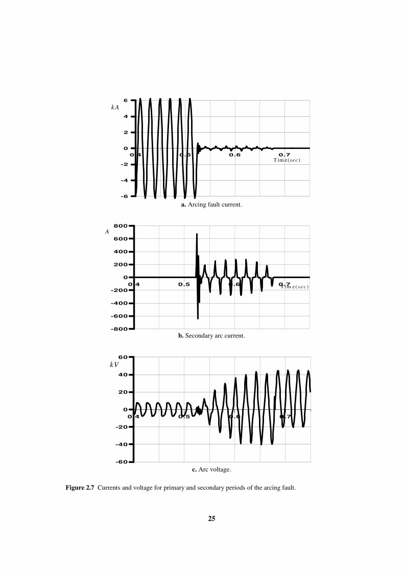
25

T im e(sec )

kA

0.4 0.5 0.6 0.7

-6

-2

2

6

-4

0

4

a. Arcing fault current.

0.4 0.5 0.6 0.7

-600

-200

200

600

-800

-400

0

400

800

A

T im e ( s e c )

b. Secondary arc current.

kV

0.4 0.5 0.6 0.7

-60

-20

20

60

-40

0

40

c. Arc voltage.

Figure 2.7 Currents and voltage for primary and secondary periods of the arcing fault.

26

27

3- Experimental Verification of High Impedance Arcing

Fault Model in MV Networks [P.II]

In order to overcome the complications of obtaining staged fault data or of studying

difficult abnormal conditions in the electrical networks, accurate fault model incorporated in

the networks at different locations reproduces the well-known fault circumstances. Fault

modeling requires experimental data to fulfill its equations and their parameters. Therefore in

this chapter, an experimental setup is used to establish a high impedance fault of a leaning tree

type. The test results are used to model the fault. The model parameters are determined. The

experimental work is implemented using the ATP/EMTP package. The tree impedance is

represented using a resistance and the arc element is modeled by a thermal model and realized

using the universal arc representation in ATPDraw.

3.1 Experimental Results

An experiment was performed to measure the characteristics of a high impedance fault

occurring in a 20 kV distribution network. The experiment was carried out at the Power

Systems and High Voltage Laboratory, Helsinki University of Technology (TKK), Finland.

Figure 3.1 shows the experimental setup. When the conductor is energized at 11.5 kV and

the tree bends close, an arc is created as shown in Figure 3.2. More details about the

experiment scenario are described in [P.II].

Towards accurate measuring, the experimental errors should be reduced. There are

several sources for these errors: errors due to transducers such as current and voltage

transformers and errors due to the reading/recording instruments such as Oscilloscopes and

recorders. Regarding the experimental work, it is carried out at High Voltage Laboratory,

TKK and the transducers in this laboratory are frequently calibrated as it can be revealed

from the appendix of Publication [P.II]. There is another issue carefully considered to

reduce the experimental error. This issue is the arrangement of these transducers (Current

and Voltage), in which the calibrated resistance is directly connected with the fault element

to accurately measure the fault current and therefore to avoid the error due to the current

injected in the voltage transducer. Then, the voltage transducer is connected across both of

the fault element and current transducer. The other point which can produce errors is the

saturation of these transducers, however, the discussed fault is a very high impedance fault

type and its disturbance is extremely small and such fault can not lead to saturation in the

utilized transducers. So during this fault, the transducers operate in the linear portions of

their characteristics.

Figure 3.3 illustrates the fault voltage and current waveforms when it is associated with

arcs at different locations over the tree. It reveals that the distortions in voltage and current

waveforms are influenced by the arc behavior. Non-steady state periods with spikes in the

voltage and current waveforms are evident at reigniting instants. This is clearly depicted in

the enlarged figures at the vicinity of the zero-crossings as shown in Figure 3.3.a.

Identification of these features can enhance this fault detection. On the other hand, the arc

28

voltage or current waveform pattern can be approximately continuous as shown in Figures

3.3.b and 3.3.c.

Arcing

Conductor

Tree

1-φ Transformer

10kVA, 0.243/20kV Source 25A

Cap

acito

r div

ider

Callibrated

resistance

Osc.

CH1 CH2

Figure 3.1 Experimental configuration.

Arcing

Figure 3.2 Arc-associated tree bending over the conductor.

29

0.055 0.06 0.065-40

0

40

80

120

0 0.02 0.04 0.06 0.08 0.1-200

-150

-100

-50

0

50

100

150

200

0.025 0.03 0.035-120

-80

-40

0

40

Time (s)

Fau

lt V

olt

ag

e a

nd

Cu

rren

t

Voltage (××××0.1kV) Current (mA)

Time (s)

Current (mA)

Voltage (××××0.1kV)

Voltage (××××0.1kV)

Current (mA)

Time (s) a. Enlarged view of waveforms and zero-crossings when the fault is in the foliage.

0 0.02 0.04 0.06 0.08 0.1-200

-150

-100

-50

0

50

100

150

200

Time (s)

Fau

lt V

olt

ag

e a

nd

Cu

rren

t Voltage (××××0.1kV)

Current (mA)

b. The waveforms when the fault is at the branch.

0 0.02 0.04 0.06 0.08 0.1-200

-150

-100

-50

0

50

100

150

200

Time (s)

Fa

ult

Vo

lta

ge a

nd

Cu

rren

t Voltage (××××0.1kV)

Current (mA)

c. The waveforms when the fault is at the trunk.

Figure 3.3 Experimental waveforms at different fault locations over the tree.

30

3.2 Modeling of the Associated Arc

To enable measuring of the arc characteristics, the arc position is experimentally

moved to a new point between the tree and the calibrated series resistance. The capacitor

divider can then be connected across the arc element to only measure the arc voltage. The

arc behavior changes from one half-cycle (power frequency) to the other as revealed by the

experimental arc characteristics shown in Figure 3.4. This constitutes one cycle specific to

an arc and it is characterized by unsymmetrical half-cycles. Therefore, the arc model

parameters extracted using the positive half-cycle are inappropriate for the other.

This arc element can be modeled using the dynamic arc equation (2.16) of long arcs.

However, the equation parameters such as the stationary arc voltage ust and arc time

constant τ are determined so as to match the experimental results. The experimental

characteristics shown in Figure 3.4 are used to determine the arc model parameters. It is

found that ust can be a fixed value while the time constant is suggested to be described as

[P.II]:

BgAe=τ (3.1)

where A and B are constants. Therefore, there are three constants to model the arc

performance. These parameters can be interpreted as which ust describes the arc voltage

clipping level. It can be determined as the arc voltage value when dg/dt=0 and it is

synchronized with the instant of maximum current occurrence. The arc hysteresis in the

simulation phase is sensitive to τ. The behavior of τ at the instant of reignition and during

the half cycle is dominated by the constant A and B, respectively. The appropriate

parameters for the positive half cycle shown in Figure 3.4 are ust = 2520 V, A = 6.6E-5 and

B = 41977 while for the negative half cycle they are ust = 2100 V, A = 2.0E-5, and B =

85970.3. The corresponding simulated arc characteristics are illustrated in the comparison

of Figure 3.5. These comparisons confirm the model accuracy.

-0.1 -0.08 -0.06 -0.04 -0.02 0 0.02 0.04 0.06 0.08 0.1-3000

-2000

-1000

0

1000

2000

3000

4000

Arcing current (A)

Arcin

g v

olt

ag

e (

V)

Positive half cycle

Negative half cycle

Figure 3.4 Experimental arc characteristics.

31

-0.1 -0.08 -0.06 -0.04 -0.02 0 0.02 0.04 0.06 0.08 0.1-4000

-3000

-2000

-1000

0

1000

2000

3000

4000

Arcing current (A)

Arcin

g v

olt

ag

e (

V)

Experimental arc

characteristics Simulated arc

characteristics

a. Fitting for the positive half cycle data.

-0.1 -0.08 -0.06 -0.04 -0.02 0 0.02 0.04 0.06 0.08 0.1-3000

-2000

-1000

0

1000

2000

3000

4000

Arcing current (A)

Arcin

g v

olt

ag

e (

V)

Experimental arc

characteristics

Simulated arc

characteristics

b. Fitting for the negative half cycle data.

Figure 3.5 Comparison of simulated with experimental arc characteristics

32

3.3 Simulation Results

The experimental system shown in Figure 3.1 was implemented using the ATP/EMTP

program where the circuit was realized using ATPDraw. Figure 3.6 shows the

corresponding ATPDraw network where it is divided into the power network to represent

the experimental setup and the TACS field to solve the dynamic arc equation. The arc

model was realized using the universal arc representation as described in [P.II]. The control

signal required for the controlled integrator and acquired from the case depicted in Figure

3.3.a is shown in Figure 3.7.a. Considering the conductance at the zero-crossing, the

dielectric of the arc medium until the instant of reignition is represented by a variable

resistance as a ramp function of 0.5 MΩ/ms for a period of 1 ms after each zero-crossing

and then 4 MΩ/ms until the reignition instant. These variables are used for matching the

experimental current and voltage waveforms until the reignition instants. They are

compromise ramp values obtained with the aid of fitting the resistance curves computed

from the experimental voltage and current during such periods. The corresponding

simulated fault waveforms are illustrated in Figure 3.7.b. In the same manner, the test case

shown in Figure 3.3.c has been simulated as shown in Figure 3.7.c. The utilized fault

parameters have been selected to be suitable for each case where the parameters Rtree, ust, A

and B are found to be 140.5 kΩ, 2520 V, 5.6E-7 and 395917 for the first simulated case,

and 130.0 kΩ, 2050 V, 8.5E-5 and 99987 for the other, respectively. In the two simulated

fault cases, the parameters A and B are compromised values for the positive and negative

half cycles. In these cases, there are differences in the arc behavior and therefore the arc

model parameters of each case are not the same. By comparing the simulated and

experimental waveforms, it appears that the fault modeling due to a leaning tree is

accurately represented.

RES

=1.0 Varc

ττττ

CT

R

R(t)

Rtree

Zs Ztr

Universal Arc

Representation

Figure 3.6 The ATPDraw network of the experimental setup

33

0 0.02 0.04 0.06 0.08 0.10

1

Time (s)

a. Control signal to distinguish dielectric and arcing periods.

0 0.02 0.04 0.06 0.08 0.1-200

-150

-100

-50

0

50

100

150

200

Time (s)

Fau

lt V

olt

ag

e a

nd

Cu

rren

t Voltage (××××0.1kV)

Current (mA)

b. The case shown in Figure 3.3.a.

0 0.02 0.04 0.06 0.08 0.1-200

-150

-100

-50

0

50

100

150

200

Time (s)

Fa

ult

Vo

ltag

e a

nd

Cu

rren

t Voltage (××××0.1kV)

Current (mA)

c. The case shown in Figure 3.3.c.

Figure 3.7 Simulation results.

34

3.4 Network Performance during the Fault

In MV networks, initial transients are generated when the networks are exposed to

disturbances such as faults. These transients are ultimately controlled by the energy

conservation theory. They are investigated to detect earth faults in unearthed and

compensated MV networks [35], [36], [45], [46]. The initial transients are in the form of

charge and discharge transient components. The discharge transient components are

happened on the faulty phase when an earth fault occurs suddenly. This gives rise to the

discharge transient component and therefore a voltage rise in the sound phases that is

accompanied by the other created components called charge transient. These initial

transients are depending on the network equivalent parameters, fault location, fault instant,

and fault impedance [35], [46]. Because the compensation coil impedance is relatively high

at the high frequencies, these transients are about similar in unearthed and compensated

networks [35].

As aforementioned, an accurate simulation of the electrical networks associated with high

impedance arcing faults is quite important to evaluate the possibility of a detection of these

faults. Using the ATP/EMTP program, the simulated system can be divided into two main

parts: the power network model and the representation of high impedance arcing fault

described in the previous section.

Figure 3.8 illustrates a single line diagram of a 20 kV, MV network. The transmission

line dependent frequency model of the EMTP program is intentionally selected to account

for the unsymmetrical faults. The feeder lines are represented using the frequency

dependent JMarti model. The neutral of the main transformer is singularly treated to

manage different earthing methods.

The residual voltage and current waveforms can be analyzed for the fault detection

purposes. They are computed as:

cbar uuuu ++= (3.2)

cbar iiii ++= (3.3)

where ir and ur are the residual current and voltage, respectively. ia , ib and ic are the phase

currents. ua , ub and uc are the phase voltages. In order to investigate these residual

waveforms during the discussed fault, the equations (3.2) and (3.3) are implemented in the

TACS field.

Figure 3.9 illustrates the ATPDraw network of the simulated system. It contains the MV

network described in Figure 3.8, the universal arc representation of the associated arc with

the tree resistance and the residual voltage and current (ur and ir) equations (3.2) and (3.3),

respectively.

35

Feeder 3 (30km)

Lf Fault point

Feeder 2 (35km)

Feeder 1 (41km) B

C

D

20/0.4kV, ∆/Υ earthed 66/20kV, ∆/Υ

Load

1.5MW, ∆

Load

1.5MW, ∆

Load

0.5MW,

Υ earthed

20/0.4kV, ∆/Υ earthed

20/0.4kV, ∆/Υ earthed Measuring

point

Feeder 5 (45km)

Feeder 4 (33km)

A

C

D

20/0.4kV, ∆/Υ earthed

Load

1.5MW, ∆

Load

1.5MW, ∆

20/0.4kV, ∆/Υ earthed

Figure 3.8 Simulated system for a substation energized 251 km distribution network.

TREE1

I

G

=1.0

U G

S3

S2S

S1F

S5

S4

RES

Varc

ττττ

CT

R

R(t)

Rtree

Universal Arc

Representation

ir

ur

L3

L2

L1

The Residual

Voltage and current

L5 L4

Figure 3.9. The ATPDraw network of the simulated system.

36

3.4.1 Unearthed Network

Although the unearthed network is not intentionally connected to the earth, it is naturally

earthed by the phase to ground capacitances. Therefore, the phase fault current is very low

and allow to a high continuity of service [30]. The main disadvantage of unearthed network

is that it is subjected to transient overvoltages.

For a fault case due to a leaning tree occurred at 27 ms at the end of Feeder 1 in an

unearthed 20 kV network depicted in Figure 3.8, the corresponding waveforms are shown

in Figure 3.10. The residual and neutral voltages are shown in Figure 3.10.a where they

ultimately depend on the fault impedance. The fault and residual currents are depicted in

Figures 3.10.b and 3.10.c, respectively. The corresponding residual current is very small

and the impact of the initial transients due to the arc reignitions is obvious after each zero-

crossing via approximately one-quarter of the power cycles as illustrated in the enlarged

view of the residual current shown in Figure 3.10.c. Therefore, it is appropriate to use a

discrete signal processing technique such as DWT to extract these transients and therefore

to localize the arc reignition instants.

3.4.2 Compensated Network

When the resonant earthing network is used, the earth fault current is correspondingly

decreased because the network earth capacitance is in a parallel resonance with the

inductance connected to the neutral. Because the neutral voltages of such networks are

substantially higher than the isolated systems, a higher sensitive relay protection for high

resistance faults can be gained [30], [35]. However, the tuning of the compensation coil is

never precise where the switching can cause major changes in the network connections. In

Nordic Countries, the compensated MV networks have increasingly been used [35].

Towards modeling the compensated network, the transmission line capacitance is

compensated by an earthed inductance of 2.85 H where it is connected at the neutral point

of main transformer in the network shown in Figure 3.8. The neutral and residual voltages

during the tree leaning fault are illustrated in Figure 3.11.a where the fault occurrence is at

the end of Feeder 1. The fault and residual currents are shown in Figure 3.11.b. The

performance of this fault is changed with different earthing although the fault impedance is

very high. However, the arc reignition fingerprints are still observed in the measured

voltage and current waveforms. The same manner is also measured when the fault location

and incipient instants are changed; however, the initial transients are affected.

Due to the fact that the impedance of the compensation coil is relatively high at high

frequencies, these transients are about similar in the unearthed and compensated networks

[35]. Regarding the high impedance arcing fault tree leaning type, these initial transients

are repeated with each arcing reignition after each current zero-crossing via approximately

one-quarter of power cycles as depicted in the residual waveforms.

37

(f ile Faulty _Sy stem3.pl4; x-v ar t) v :NEUTR t: U.R

0.00 0.03 0.06 0.09 0.12 0.15[s]-300

-200

-100

0

100

200

300

400

500

Time (sec)

Vo

ltage (

V)

ur

un

a. Measured neutral voltage (un) and residual voltage (ur).

(f ile Faulty _Sy stem3.pl4; x-v ar t) c:FA -TREE1

0.00 0.03 0.06 0.09 0.12 0.15[s]-90

-60

-30

0

30

60

90

[mA]

Time (sec)

Cu

rren

t (m

A)

b. Fault current (if)

(f ile Faulty _Sy stem3.pl4; x-v ar t) t: I.R

0.00 0.03 0.06 0.09 0.12 0.15[s]-0.08

-0.04

0.00

0.04

0.08

0.12

Time (sec)

Cu

rren

t (A

)

(f ile Faulty _Sy stem3.pl4; x-v ar t) t: I.R

45 49 53 57 61 65[ms]-80

-60

-40

-20

0

20

40

60

80*10 -3

Time (sec)

Cu

rren

t (m

A)

c. Enlarged view of residual current waveforms (ir)

Figure 3.10 The transient waveforms when the network is unearthed.

38

0.00 0.04 0.08 0.12 0.16 0.20[s]-1500

-1000

-500

0

500

1000

1500

Time (sec)

Vo

ltage (

V)

ur

un

a. Neutral and residual voltages (un and ur, respectively).

0.00 0.04 0.08 0.12 0.16 0.20[s]-0.16

-0.08

0.00

0.08

0.16

Time (sec)

Cu

rren

t (A

)

if

ir

b. Fault and residual currents (if and ir, respectively).

Figure 3.11 The waveforms when the fault occurs at the end of Feeder 1 on the compensated earth network.

39

4- DWT-Based Investigation of Network Currents for

Detecting High Impedance Arcing Fault [P.III], [P.IV]

In this chapter, the impact of the arc reignition periodicity on the network currents is

utilized to detect the faults due to leaning trees. In the vicinity of the current zero-crossing,

the initial transients lead to fingerprints boosting secure fault detections. These transients

are localized based on the DWT detail coefficient of the feeder currents to detect the fault.

The fault detector is based on the absolute sum of the DWT detail coefficient over one

power cycle. The selectivity function to estimate the faulty feeder or the faulty phase is

based on Logic Functions where their inputs are the absolute sum of the DWT detail

coefficients as reported in [P.III]. However, when the currents are measured not only at the

main busbar but also at different measuring nodes throughout the network, another

selectivity function is introduced based on the residual current ratio as addressed in [P.IV].

The ratio of the residual fundamental current of each section with respect to the

fundamental current of parent section in the feeder is used as a discriminator to estimate the

faulty section.

4.1 Feature Extraction and Fault Detection Algorithm using DWT [P.III]

The scenario of the fault detection and the faulty feeder estimation is illustrated in

Figure 4.1. At the measuring node of each feeder, phase currents are measured and the fault

features are extracted using DWT. The absolute sum of the detail d3 coefficient

corresponding to the frequency band 12.5-6.25 kHz is computed over one cycle period of

the power frequency for the fault detection purpose. The sampling frequency is 100 kHz. A

timer is used to determine the fault period and it can be implemented using a samples

counter. In order to find out the faulty phase, the absolute sum over one power cycle of the

detail d3 of each phase is evaluated using a Logic Function, in which, the absolute sum of

the faulty phase is the highest one when it is compared with the absolute sum of other

phases. A similar feature is found when a comparison between the absolute sums of the

feeders for the same phase current where the absolute sum of the faulty feeder is the highest

one. Therefore, another Logic Function is designed to determine the faulty feeder. The

selectivity of the faulty phase and feeder is taken into consideration after the fault detection

is achieved. More details about the algorithm can be found in [P.III].

Several wavelet families have been tested to extract the fault features using the

Wavelet toolbox incorporated into the MATLAB program [106]. It is found that

Daubechies wavelet 14 (db14) is appropriate to localize this fault, in which characteristics

of Daubechies wavelets (dbN) are arbitrary regular, compactly supported orthogonal and

asymmetry. When the sampling frequency is equal to 100 kHz, the corresponding

frequency distribution for each detail level is shown in Figure 4.2. The Detail d3 including

the frequency band 12.5-6.25 kHz is investigated. The sampling rate can be reduced to 50

40

or 25 kHz but the used coefficients will be details d2 or d1, respectively. More reduction in

the sampling frequency can be considered, however, the absolute sum detector has less

gain.

For the tree leaning fault case occurred at the end of Feeder 1 of the network shown in

Figure 3.8, extracted features from the phase current waveforms measured for different

feeders using DWT are shown in Figure 4.3. This fault case started at 26 ms. The initial

transients due to arc reignitions are frequently localized throughout the network feeders.

Start

Currents at the

measuring node of

the Feeder j

Currents (ia, ib, ic)

DWT

Features Extraction

Absolute sum over one power cycle

SIa, Ib, Ic (Feeder j)

Fault Detection

If

SI > 0.01

No

Yes

Detector

ia-j

Detail d3

1

1

1 Timer

ib-j ic-j Phase currents

of the feeder number j

d3Ia(Feeder j) d3Ib(Feeder j) d3Ic(Feeder j)

Logic

Function 2

Logic

Function 1

Faulty Phase Faulty Feeder

SIa, Ib, Ic (Feeder j)

Figure 4.1 The proposed detection technique.

Input(k)

at 100 kHz LF

HF

LF

HF

2 LF 2

HF

d1

d2

a6

d6

50kHz

25kHz

12.5kHz

781.25Hz

0

1.562kHz

2

2

Figure 4.2 Dyadic wavelet analysis filter bank.

41

0 0.02 0.04 0.06 0.08 0.1 0.12 0.14 0.16-0.05

0

0.05

d3Ia(Feeder1)

0 0.02 0.04 0.06 0.08 0.1 0.12 0.14 0.16-0.02

0

0.02

d3Ib(Feeder1)

0 0.02 0.04 0.06 0.08 0.1 0.12 0.14 0.16-0.02

0

0.02

d3Ic(Feeder1)

0 0.02 0.04 0.06 0.08 0.1 0.12 0.14 0.16-0.01

0

0.01

d3Ia(Feeder2)

0 0.02 0.04 0.06 0.08 0.1 0.12 0.14 0.16-5

0

5x 10

-3 d3Ib(Feeder2)

0 0.02 0.04 0.06 0.08 0.1 0.12 0.14 0.16-5

0

5x 10

-3 d3Ic(Feeder2)

a. Details d3 of phase currents of Feeder 1. b. Details d3 of phase currents of Feeder 2.

0 0.02 0.04 0.06 0.08 0.1 0.12 0.14 0.16-0.02

0

0.02

d3Ia(Feeder3)

0 0.02 0.04 0.06 0.08 0.1 0.12 0.14 0.16-0.01

0

0.01

d3Ib(Feeder3)

0 0.02 0.04 0.06 0.08 0.1 0.12 0.14 0.16-0.01

0

0.01

d3Ic(Feeder3)

0 0.02 0.04 0.06 0.08 0.1 0.12 0.14 0.16-5

0

5x 10

-3 d3Ia(Feeder4)

0 0.02 0.04 0.06 0.08 0.1 0.12 0.14 0.16-5

0

5x 10

-3 d3Ib(Feeder4)

0 0.02 0.04 0.06 0.08 0.1 0.12 0.14 0.16-5

0

5x 10

-3 d3Ic(Feeder4)

c. Details d3 of phase currents of Feeder 3. d. Details d3 of phase currents of Feeder 4.

0 0.02 0.04 0.06 0.08 0.1 0.12 0.14 0.16-0.02

0

0.02

d3Ia(Feeder5)

0 0.02 0.04 0.06 0.08 0.1 0.12 0.14 0.16-0.01

0

0.01

d3Ib(Feeder5)

0 0.02 0.04 0.06 0.08 0.1 0.12 0.14 0.16-0.01

0

0.01

d3Ic(Feeder5)

e. Details d3 of phase currents of Feeder 5.

Figure 4.3 Details d3 of phase currents at a beginning of the network feeders.

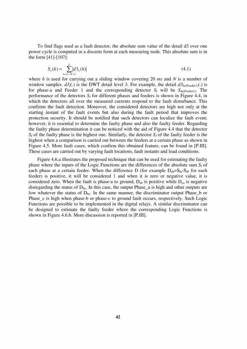
42

To find flags used as a fault detector, the absolute sum value of the detail d3 over one

power cycle is computed in a discrete form at each measuring node. This absolute sum is in

the form [41]-[107]:

∑+−=

=k

Nkh

II hdkS1

)(3)( (4.1)

where h is used for carrying out a sliding window covering 20 ms and N is a number of

window samples. d3I(.) is the DWT detail level 3. For example, the detail d3Ia(Feeder1)(.) is

for phase-a and Feeder 1 and the corresponding detector SI will be SIa(Feeder1). The

performance of the detectors SI for different phases and feeders is shown in Figure 4.4, in

which the detectors all over the measured currents respond to the fault disturbance. This

confirms the fault detection. Moreover, the considered detectors are high not only at the

starting instant of the fault events but also during the fault period that improves the

protection security. It should be notified that such detectors can localize the fault event;

however, it is essential to determine the faulty phase and also the faulty feeder. Regarding

the faulty phase determination it can be noticed with the aid of Figure 4.4 that the detector

SI of the faulty phase is the highest one. Similarly, the detector SI of the faulty feeder is the

highest when a comparison is carried out between the feeders at a certain phase as shown in

Figure 4.5. More fault cases, which confirm this obtained feature, can be found in [P.III].

These cases are carried out by varying fault locations, fault instants and load conditions.

Figure 4.6.a illustrates the proposed technique that can be used for estimating the faulty

phase where the inputs of the Logic Functions are the differences of the absolute sum SI of

each phase at a certain feeder. When the difference D (for example Dab=SIa-SIb for each

feeder) is positive, it will be considered 1 and when it is zero or negative value, it is

considered zero. When the fault is phase-a to ground, Dab is positive while Dca is negative

disregarding the status of Dbc. In this case, the output Phase_a is high and other outputs are

low whatever the status of Dbc. In the same manner, the discriminator output Phase_b or

Phase_c is high when phase-b or phase-c to ground fault occurs, respectively. Such Logic

Functions are possible to be implemented in the digital relays. A similar discriminator can

be designed to estimate the faulty feeder where the corresponding Logic Functions is

shown in Figure 4.6.b. More discussion is reported in [P.III].

43

0.02 0.04 0.06 0.08 0.1 0.12 0.14 0.160

0.1

0.2

0.3

0.4

SI(Feeder1)

SIa(Feeder1)

SIb(Feeder1)

SIc(Feeder1)

0.02 0.04 0.06 0.08 0.1 0.12 0.14 0.160

0.05

0.1

0.15

0.2

SI(Feeder2)

SIa(Feeder2)

SIb(Feeder2)

SIc(Feeder2)

0.02 0.04 0.06 0.08 0.1 0.12 0.14 0.160

0.05

0.1

0.15

0.2

SI(Feeder3)

SIa(Feeder3)

SIb(Feeder3)

SIc(Feeder3)

0.02 0.04 0.06 0.08 0.1 0.12 0.14 0.160

0.05

0.1

0.15

0.2

SI(Feeder4)

SIa(Feeder4)

SIb(Feeder4)

SIc(Feeder4)

0.02 0.04 0.06 0.08 0.1 0.12 0.14 0.160

0.05

0.1

0.15

0.2

SI(Feeder5)

SIa(Feeder5)

SIb(Feeder5)

SIc(Feeder5)

Figure 4.4 The detector SI of different phases (SIa, SIb and SIc) at the beginning of certain feeder.

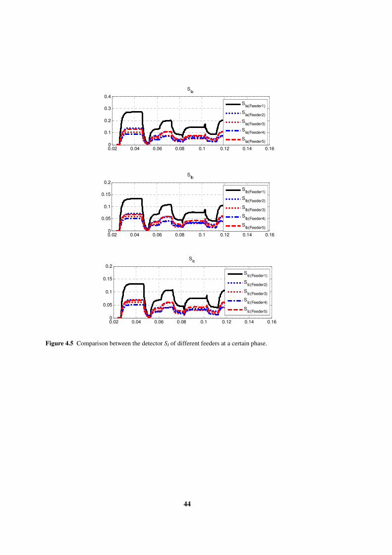
44

0.02 0.04 0.06 0.08 0.1 0.12 0.14 0.160

0.1

0.2

0.3

0.4

SIa

SIa(Feeder1)

SIa(Feeder2)

SIa(Feeder3)

SIa(Feeder4)

SIa(Feeder5)

0.02 0.04 0.06 0.08 0.1 0.12 0.14 0.160

0.05

0.1

0.15

0.2

SIb

SIb(Feeder1)

SIb(Feeder2)

SIb(Feeder3)

SIb(Feeder4)

SIb(Feeder5)

0.02 0.04 0.06 0.08 0.1 0.12 0.14 0.160

0.05

0.1

0.15

0.2

SIc

SIc(Feeder1)

SIc(Feeder2)

SIc(Feeder3)

SIc(Feeder4)

SIc(Feeder5)

Figure 4.5 Comparison between the detector SI of different feeders at a certain phase.

45

Dab= SIa - SIb

Dbc= SIb - SIc

Dca= SIc - SIa

SIa

Difference between

the absolute sum.

Dab Dbc Dca

Phase_a

SIb SIc

Phase_a=Dab AND NOT Dca

Phase_b=Dbc AND NOT Dab

Phase_c=Dca AND NOT Dbc

Faulty Phase Phase_b Phase_c

Logic Functions

for determining

the faulty phase

Absolute sum of

the phase currents

a. Faulty phase Discriminator.

D12= SI(Feeder 1) – SI(Feeder 2)

D23= SI(Feeder 2) – SI(Feeder 3)

D34= SI(Feeder 3) – SI(Feeder 4)

D45= SI(Feeder 4) – SI(Feeder 5)

D51= SI(Feeder 5) – SI(Feeder 1)

D13= SI(Feeder 1) – SI(Feeder 3)

D35= SI(Feeder 3) – SI(Feeder 5)

D52= SI(Feeder 5) – SI(Feeder 2)

D24= SI(Feeder 2) – SI(Feeder 4)

D41= SI(Feeder 4) – SI(Feeder 1)

SI(Feeder 1)

Difference between

the absolute sum

D12 D23 D34

Feeder_1

Feeder_1= D12 AND D13 AND NOT D41 AND NOT D51

Feeder_2= D23 AND D24 AND NOT D52 AND NOT D12

Feeder_3= D34 AND D35 AND NOT D13 AND NOT D23

Feeder_4= D45 AND D41 AND NOT D24 AND NOT D34

Feeder_5= D51 AND D52 AND NOT D35 AND NOT D45

Faulty Feeder Feeder_2 Feeder_3

Logic Functions for

determining the

faulty feeder

Absolute sum of the

feeders of certain

phase current

SI(Feeder 2) SI(Feeder 3) SI(Feeder 4) SI(Feeder 5)

D45 D51 D13 D13 D51 D13 D13

Feeder_4 Feeder_5

b. Faulty feeder discriminator.

Figure 4.6 The proposed Selectivity Function.

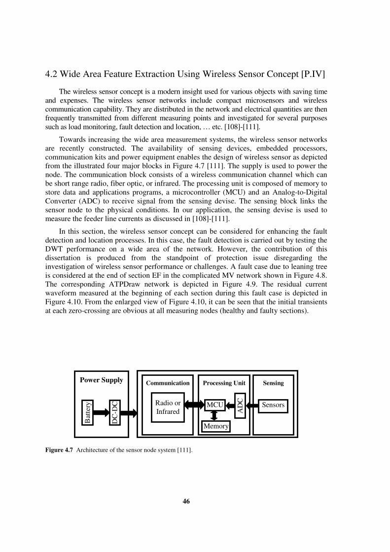
46

4.2 Wide Area Feature Extraction Using Wireless Sensor Concept [P.IV]

The wireless sensor concept is a modern insight used for various objects with saving time

and expenses. The wireless sensor networks include compact microsensors and wireless

communication capability. They are distributed in the network and electrical quantities are then

frequently transmitted from different measuring points and investigated for several purposes

such as load monitoring, fault detection and location, … etc. [108]-[111].

Towards increasing the wide area measurement systems, the wireless sensor networks

are recently constructed. The availability of sensing devices, embedded processors,

communication kits and power equipment enables the design of wireless sensor as depicted

from the illustrated four major blocks in Figure 4.7 [111]. The supply is used to power the

node. The communication block consists of a wireless communication channel which can

be short range radio, fiber optic, or infrared. The processing unit is composed of memory to

store data and applications programs, a microcontroller (MCU) and an Analog-to-Digital

Converter (ADC) to receive signal from the sensing devise. The sensing block links the

sensor node to the physical conditions. In our application, the sensing devise is used to

measure the feeder line currents as discussed in [108]-[111].

In this section, the wireless sensor concept can be considered for enhancing the fault

detection and location processes. In this case, the fault detection is carried out by testing the

DWT performance on a wide area of the network. However, the contribution of this

dissertation is produced from the standpoint of protection issue disregarding the

investigation of wireless sensor performance or challenges. A fault case due to leaning tree

is considered at the end of section EF in the complicated MV network shown in Figure 4.8.

The corresponding ATPDraw network is depicted in Figure 4.9. The residual current

waveform measured at the beginning of each section during this fault case is depicted in

Figure 4.10. From the enlarged view of Figure 4.10, it can be seen that the initial transients

at each zero-crossing are obvious at all measuring nodes (healthy and faulty sections).

Power Supply

Bat

tery

DC

-DC

Communication

Radio or

Infrared

Processing Unit

MCU

Memory

AD

C

Sensing

Sensors

Figure 4.7 Architecture of the sensor node system [111].

47

Fault

point

5 km

D 66/20kV, ∆/Υ

Load

A Other 4 feeders with

summation length

equal to 198 km

5 km

5 km

7 km

4 km

Load

Load

10 km

Load

7 km

5 km

B

C

Load

Load

E

K

F

5 km

Wireless

sensors H

I

J

Circuit

Breaker

Figure 4.8 Simulated system for a substation energized 251 km distribution network.

TREE1

I=1.0

U

E

F

B

C

K

D H

I

JA

RES

Varc

ττττ

CT

R

R(t)

Rtree

Universal Arc

Representation

ir(AB)

Feeder 3

Feeder 2

Feeder 1

Feeder 5

Feeder 4

66/20kV

Transformer

ir(BE)

ir(EF)

ur(A)

ur(B)

ur(D)

ir(Feeder 5)

ir(Feeder 4)

ir(Feeder 3)

ir(Feeder 2)

Figure 4.9 The ATPDraw network

48

Features of the residual currents shown in Figure 4.10 are extracted using DWT. In the

same manner, the sampling frequency is 100 kHz and the mother wavelet is Daubechies

wavelet 14 (db14). Figure 4.11 illustrates the corresponding detail levels d3, d4 and d5. The

detectors SIr performance is evaluated and shown in Figure 4.12, in which, the fault is

detected based on DWT. Furthermore, the detectors are high not only at the fault starting

instant but also during the fault period which enhances the fault detection security. As

aforementioned, such performance is due the arc reignitions after each fault current zero-

crossing. Towards decreasing the sampling frequency at which the DWT is processed,

when the detectors SIr of the DWT detail d4, which is indicated SIr(d4), is considered a

detector, the sampling frequency can be reduced to 50, 25 or 12.5 kHz; however, the used

coefficient will be detail d3, d2, or d1, respectively. However, the faulty section cannot be

discriminated using the detectors SIr.

0.00 0.03 0.06 0.09 0.12 0.15[s]-0.090

-0.052

-0.014

0.024

0.062

0.100

39 40 41 42 43 44 45 46 47[ms]-20

2

24

46

68

90

*10 -3

Time (sec)

Cu

rren

t (A

)

Time (ms)

Cu

rren

t (m

A)

ir(AB)

ir(EF) ir(BE)

ir of the healthy sections

Figure 4.10 Enlarged view of residual current waveforms (ir) when the fault occurred in section EF.

49

0 0.02 0.04 0.06 0.08 0.1 0.12 0.14 0.16-5

0

5

10x 10

-3 d3

0 0.02 0.04 0.06 0.08 0.1 0.12 0.14 0.16-0.05

0

0.05d4

0 0.02 0.04 0.06 0.08 0.1 0.12 0.14 0.16-0.1

0

0.1d5

sec

sec

sec

a. Details of the residual current in section AB (ir(AB))

0 0.02 0.04 0.06 0.08 0.1 0.12 0.14 0.16-0.01

0

0.01d3

0 0.02 0.04 0.06 0.08 0.1 0.12 0.14 0.16-0.05

0

0.05d4

0 0.02 0.04 0.06 0.08 0.1 0.12 0.14 0.16-0.02

0

0.02d5

sec

sec

sec

(b) Details of the residual current in section BC (ir(BC))

0 0.02 0.04 0.06 0.08 0.1 0.12 0.14 0.16-5

0

5x 10

-3 d3

0 0.02 0.04 0.06 0.08 0.1 0.12 0.14 0.16-0.1

0

0.1d4

0 0.02 0.04 0.06 0.08 0.1 0.12 0.14 0.16-0.1

0

0.1d5

sec

sec

sec

c. Details of the residual current in section BD (ir(BD))

0 0.02 0.04 0.06 0.08 0.1 0.12 0.14 0.16-0.02

0

0.02d3

0 0.02 0.04 0.06 0.08 0.1 0.12 0.14 0.16-0.1

0

0.1d4

0 0.02 0.04 0.06 0.08 0.1 0.12 0.14 0.16-0.1

0

0.1d5

sec

sec

sec

d. Details of the residual current in section BE (ir(BE))

0 0.02 0.04 0.06 0.08 0.1 0.12 0.14 0.16-0.05

0

0.05d3

0 0.02 0.04 0.06 0.08 0.1 0.12 0.14 0.16-0.05

0

0.05d4

0 0.02 0.04 0.06 0.08 0.1 0.12 0.14 0.16-0.02

0

0.02d5

sec

sec

sec

e. Details of the residual current in section EK (ir(EK))

0 0.02 0.04 0.06 0.08 0.1 0.12 0.14 0.16-0.05

0

0.05d3

0 0.02 0.04 0.06 0.08 0.1 0.12 0.14 0.16-0.05

0

0.05d4

0 0.02 0.04 0.06 0.08 0.1 0.12 0.14 0.16-0.1

0

0.1d5

sec

sec

sec

f. Details of the residual current in section EF (ir(EF))

Figure 4.11 Details of residual waveforms shown in Figure 4.10.

b.

50

0 0.02 0.04 0.06 0.08 0.1 0.12 0.14 0.160

0.2

0.4

0.6

0.8

0 0.02 0.04 0.06 0.08 0.1 0.12 0.14 0.160

0.1

0.2

0.3

0.4

sec

sec (a) Sdi of the residual current details in section AB (ir(AB))

(b) Sdi of the residual current details in section BC (ir(BC))

Sd5

Sd4

Sd3

Sd4

Sd3

Sd5

0 0.02 0.04 0.06 0.08 0.1 0.12 0.14 0.160

0.2

0.4

0.6

0.8

0 0.02 0.04 0.06 0.08 0.1 0.12 0.14 0.160

0.2

0.4

0.6

0.8

1

sec

sec (c) Sdi of the residual current details in section BD (ir(BD))

(d) Sdi of the residual current details in section BE (ir(BE))

Sd4

Sd3

Sd5

Sd4

Sd5

Sd3

0 0.02 0.04 0.06 0.08 0.1 0.12 0.14 0.160

0.1

0.2

0.3

0.4

0 0.02 0.04 0.06 0.08 0.1 0.12 0.14 0.160

0.2

0.4

0.6

0.8

sec

sec (e) Sdi of the residual current details in section EK (ir(EK))

(f) Sdi of the residual current details in section EF (ir(EF))

Sd4

Sd3

Sd5

Sd5

Sd4

Sd3

Figure 4.12 The detector SIr of the details shown in Figure 4.11.

SIr(d5)

SIr(d5)

SIr(d5)

SIr(d5)

SIr(d5)

SIr(d5)

SIr(d4)

SIr(d4)

SIr(d4)

SIr(d4)

SIr(d4)

SIr(d4)

SIr(d3)

SIr(d3)

SIr(d3)

SIr(d3)

SIr(d3)

SIr(d3)

a. SIr

b. SIr

c. SIr

d. SIr

e. SIr

f. SIr

51

There is an observation obtained from Figure 4.10 is that the highest residual current

amplitude is the measured one in the faulty section and in the upstream sections BE and

AB. Therefore, this observation is exploited to introduce another selectivity function

because it is difficult to design Logic Functions with a high number of measuring nodes.

The proposed selectivity function depends on the ratio of the fundamental component of

each section with respect to the parent section AB. Therefore, the fundamental component

has to be tracked using a signal processing technique such Discrete Fourier Transform

(DFT). The recursive DFT is in the form:

)cos())()((2

)1()( θkNkikiN

kIkI rrrealreal −−+−= (8)

)sin2

)1()( (kθN))(ki(k)(iN

kIkI rrimajimaj −−+−= (9)

)()()( kIkIkI imajrealr

22 += (10)

where θ = 2π/N, ir(.) is the discrete input samples of the residual current. Ireal(.), Iimaj(.) and

Ir(.) are the in-phase, quadrature-phase and residual current amplitude, respectively. The

corresponding fundamental amplitudes of the residual current waveforms of different

sections are shown in Figure 4.13. It illustrates that the residual current amplitudes of

sections AB, BE and EF are higher than the others. Accordingly, the ratio of the residual

fundamental current component of each section with respect to the residual current

amplitude of the parent section AB is computed to estimate the fault path. For example, the

ratio regarding section EK is:

)AB(

)EK(

EK

r

r

I

IR = (4.4)

where Ir(EK) and Ir(AB) are the fundamental residual current components of sections EK and

AB, respectively. Similarly, the ratios regarding other sections are computed and their

performance is shown in Figure 4.14. Because the fault is in section EF, the ratios RBE and

REF are the highest and they are approximately close to one during the fault. Before the

fault, the ratios are not stable because the value of residual current of section AB is

approximately zero. However, they are only considered when the fault existed where the

fault existence can be ascertained using the detector SIr.

Towards increasing the fault location security, the aforementioned ratio is computed for

the change of residual current amplitudes. This change is the difference between the

residual current magnitude during and pre-fault measuring. However, such selectivity

function needs to discriminate between pre and during-fault periods where this task can be

carried out using the detector SIr. Furthermore, synchronization between the measured

currents should be attained. This synchronization can also be achieved by evaluating the

detector SIr performance throughout the network where the DWT details are responded to

the fault event simultaneously at different measuring nodes.

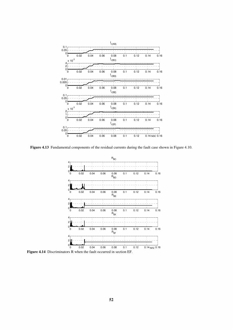
52

0 0.02 0.04 0.06 0.08 0.1 0.12 0.14 0.160

0.050.1

Ir(AB)

0 0.02 0.04 0.06 0.08 0.1 0.12 0.14 0.16024

x 10-3 I

r(BC)

0 0.02 0.04 0.06 0.08 0.1 0.12 0.14 0.160

0.0050.01

Ir(BD)

0 0.02 0.04 0.06 0.08 0.1 0.12 0.14 0.160

0.050.1

Ir(BE)

0 0.02 0.04 0.06 0.08 0.1 0.12 0.14 0.16012

x 10-3 I

r(EK)

0 0.02 0.04 0.06 0.08 0.1 0.12 0.14 0.160

0.050.1

Ir(EF)

sec

Figure 4.13 Fundamental components of the residual currents during the fault case shown in Figure 4.10.

0 0.02 0.04 0.06 0.08 0.1 0.12 0.14 0.160

2

4

RBC

0 0.02 0.04 0.06 0.08 0.1 0.12 0.14 0.160

2

4

RBD

0 0.02 0.04 0.06 0.08 0.1 0.12 0.14 0.160

2

4

RBE

0 0.02 0.04 0.06 0.08 0.1 0.12 0.14 0.160

2

4

REK

0 0.02 0.04 0.06 0.08 0.1 0.12 0.14 0.160

2

4

REF

sec Figure 4.14 Discriminators R when the fault occurred in section EF.

53

5- DWT-Based Power Direction Selectivity of High

Impedance Arcing Fault Detection [P.V], [P.VI]

Figure 5.1 shows another detection procedure proposed in this dissertation where it is

also depending on DWT. However in this case, the network voltages and currents are taken

at each measuring node. The fault features are extracted using DWT. The absolute sum,

however, of the phase voltage detail d3 coefficient over one cycle period of the power

frequency is estimated for fault detection purposes. A threshold value of 1.0 is suggested to

discriminate the fault features from measurement noise, as described in [P.V]. This

threshold value is better than the previous one suggested when the current waveforms were

considered as in [P.III], [P.IV]. In order to determine the faulty feeder, the detail d3 of the

voltage and current of each connected feeder are together multiplied to compute the power.

Using the sum over a period of two power cycles, the power direction in the form of its

polarity is utilized to identify the faulty feeder. When this power is negative, the fault

occurrence is in the corresponding feeder; however, when it is positive the feeder is

healthy. In a general form, when the fault features appear on the voltage details, the fault

tracking process is considered. From the practical point of view, there is more challenge for

detecting the faults due to leaning trees in MV networks. This challenge is due to the

network noise. The main point to verify the detection possibility is applying the proposed

technique on staged fault cases as evaluated in this chapter.

Start

Currents and voltages at

the measuring node

Currents (ia, ib, ic)

DWT

Features Extraction

d3U

Absolute sum over

one power cycle

SU

Fault Detection and fault

tracking consideration

If

SU > 1.0

No

Yes

Detector

d3U ΧΧΧΧ d3I

The Fault is in

this Feeder

Voltages (ua, ub, uc)

(ua, ub, uc) (ia, ib, ic)

d3I Detail d3 of the

voltages

Sum over two

power cycles

1

1

1 Timer 1

Detail d3 of the

currents

Check

the Polarity

-ve

+ve

The Fault is not

in this Feeder

1

Transient power over

a frequency band of

detail d3

d3U

Figure 5.1 The flowchart for the detection technique implementation.

54

5.1 Feature Extraction from Phase Quantities [P.V]

Daubechies mother wavelet 14 (db14) and the details d3 are also used in this section for

localizing the fault with a sampling frequency of 100 kHz. For the fault case occurred at the

end of Feeder 1 in the network shown in Figure 3.8, the fault features are extracted from the

phase voltages as shown in Figure 5.2. Also, the initial transients due to arc reignitions are

frequently localized in the healthy and faulty phase voltage details. Using the voltage

details in preference to current details, a performance of the detector SU, which is the

absolute sum value of the phase voltages, is shown in Figure 5.3. The performance of SU

ensures the fault detection.

A performance of the proposed discriminator method to estimate the faulty feeder can be

ensured by Figure 5.4. The details d3 of the voltage and currents of the healthy feeders are

in-phase. However, the detail of the faulty feeder current is out of phase. Such shifting can

be tracked by multiplying the details of the voltage (d3U) and current (d3I) for each phase of

each feeder. It can be considered as the harmonic-band power over the frequency range

12.5-6.25 kHz. The power polarity is estimated using summation over a period of two

cycles. As an example, this power for phase-a and for Feeder j is:

( )∑+−=

=k

Nkh

jFeederIaUajFeedera hdhdkP12

)()( )(3)(3)( (5.1)

where Pa(Feeder j)(.) is used as a discriminator where its polarity is used to point out the fault

point. The discriminator performance is shown in Figure 5.5. The discriminator polarity is

positive for healthy feeders and negative for faulty Feeder 1 as confirmed for each phase.

However, the faulty phase is not determined. Therefore, the proposed technique can be used

considering the residual components (voltage and currents) as described in the following

section.

0 0.02 0.04 0.06 0.08 0.1 0.12 0.14 0.16 0.18 0.2-2

0

2

d3Va

0 0.02 0.04 0.06 0.08 0.1 0.12 0.14 0.16 0.18 0.2-2

0

2

d3Vb

0 0.02 0.04 0.06 0.08 0.1 0.12 0.14 0.16 0.18 0.2-2

0

2

d3Vc

Time(s)

d3Ua

d3Ub

d3Uc

Time (s)

Figure 5.2 Details d3 of the phase voltages.

55

0.02 0.04 0.06 0.08 0.1 0.12 0.14 0.16 0.18 0.20

5

10

15

20

25

30

35

SV

SVa

SVb

SVc

Time (s)

SU

SUa

SUb

SUc

Figure 5.3 The detector SU performance using the phase voltage details.

0.0525 0.0526 0.0527 0.0528 0.0529 0.053 0.0531 0.0532

-1

-0.5

0

0.5

1

Time(s)

d3Va

d3Ia(Feeder1)

d3Ia(Feeder2)

d3Ia(Feeder3)

d3Ia(Feeder4)

d3Ia(Feeder5)

d3Ua

d3Ia(Feeder1)

d3Ia(Feeder2)

d3Ia(Feeder3)

d3Ia(Feeder4)

d3Ia(Feeder5)

Figure 5.4 Enlarged view of phase-a voltage and feeder current details.

56

0 0.02 0.04 0.06 0.08 0.1 0.12 0.14 0.16 0.18 0.2-0.06

-0.05

-0.04

-0.03

-0.02

-0.01

0

0.01

0.02

0.03

Pa(Feeder1)

Pa(Feeder2)

Pa(Feeder3)

Pa(Feeder4)

Pa(Feeder5)

Time (s)

a. Comparison for phase-a.

0 0.02 0.04 0.06 0.08 0.1 0.12 0.14 0.16 0.18 0.2-0.06

-0.05

-0.04

-0.03

-0.02

-0.01

0

0.01

0.02

0.03

Pb(Feeder1)

Pb(Feeder2)

Pb(Feeder3)

Pb(Feeder4)

Pb(Feeder5)

Time (s)

b. Comparison for phase-b.

0 0.02 0.04 0.06 0.08 0.1 0.12 0.14 0.16 0.18 0.2-0.06

-0.05

-0.04

-0.03

-0.02

-0.01

0

0.01

0.02

0.03

Pc(Feeder1)

Pc(Feeder2)

Pc(Feeder3)

Pc(Feeder4)

Pc(Feeder5)

Time (s)

c. Comparison for phase-c.

Figure 5.5 Comparison between the discriminator Pa, Pb, and Pc of the different feeders.

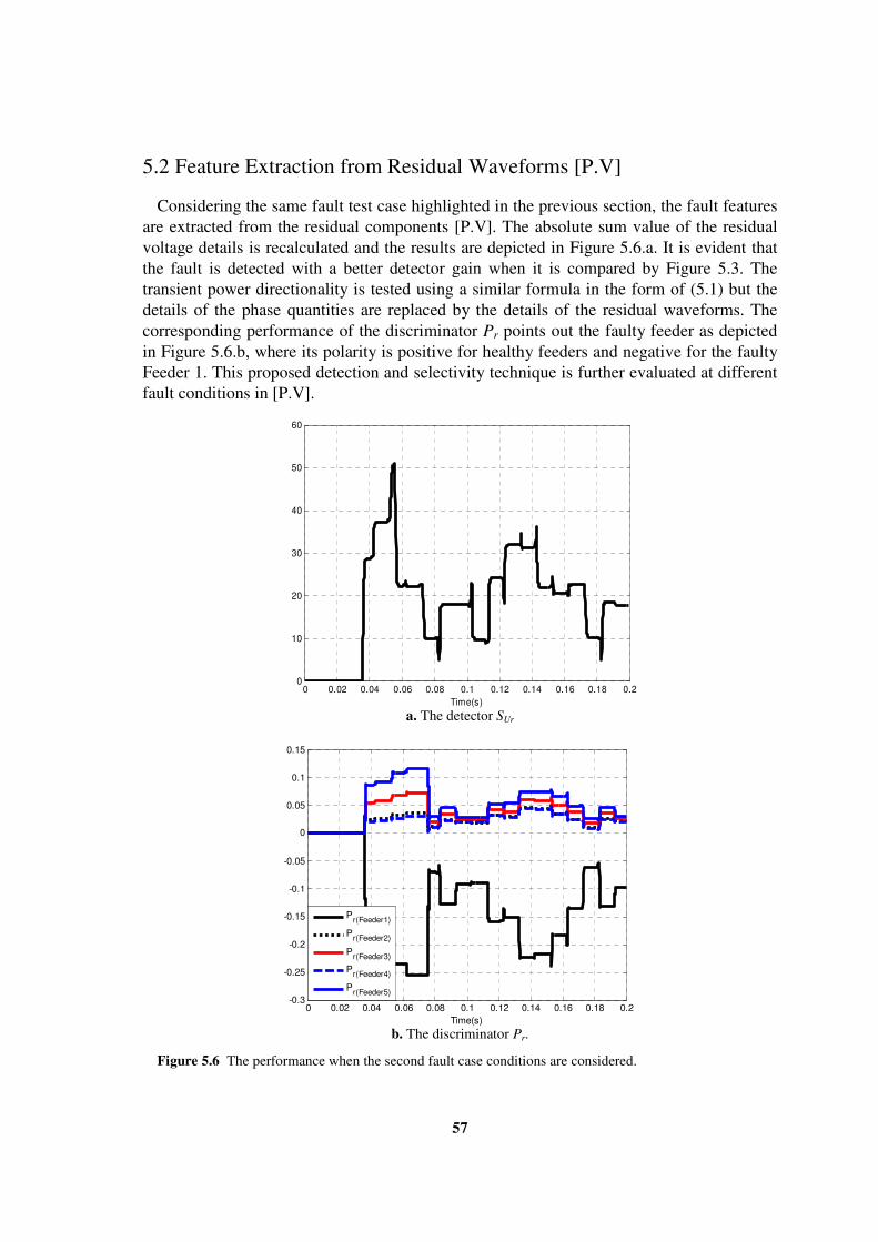
57

5.2 Feature Extraction from Residual Waveforms [P.V]

Considering the same fault test case highlighted in the previous section, the fault features

are extracted from the residual components [P.V]. The absolute sum value of the residual

voltage details is recalculated and the results are depicted in Figure 5.6.a. It is evident that

the fault is detected with a better detector gain when it is compared by Figure 5.3. The

transient power directionality is tested using a similar formula in the form of (5.1) but the

details of the phase quantities are replaced by the details of the residual waveforms. The

corresponding performance of the discriminator Pr points out the faulty feeder as depicted

in Figure 5.6.b, where its polarity is positive for healthy feeders and negative for the faulty

Feeder 1. This proposed detection and selectivity technique is further evaluated at different

fault conditions in [P.V].

0 0.02 0.04 0.06 0.08 0.1 0.12 0.14 0.16 0.18 0.20

10

20

30

40

50

60

Time(s)

a. The detector SUr

0 0.02 0.04 0.06 0.08 0.1 0.12 0.14 0.16 0.18 0.2-0.3

-0.25

-0.2

-0.15

-0.1

-0.05

0

0.05

0.1

0.15

Time(s)

Pr(Feeder1)

Pr(Feeder2)

Pr(Feeder3)

Pr(Feeder4)

Pr(Feeder5)

b. The discriminator Pr.

Figure 5.6 The performance when the second fault case conditions are considered.

58

5.3 Field Data Verification

When the fault object has a high resistance such as tree, the fault detection possibility is

reduced because its impact on the network waveforms can not be easily recognized. In such

fault cases, the fault features are very small and the network noise can also contribute to

loss of the fault detection (or loss of dependability of the fault detection). The only method

which can confirm the high impedance fault detection is to evaluate the detection

techniques using field data either using actual fault cases or considering staged faults. In

this section, the proposed technique introduced at the beginning of this chapter is examined

using staged fault cases.

In November 1995, staged earth faults were accomplished in a 20 kV network using

known fault resistances and also using natural trees. The network was only two feeders.

However, these fault cases were not associated with arcs. Figure 5.7 shows a wire

connection between the network conductor and the fault object which was a tree where it

was connected to the faulty feeder before its energizing. Then, the breaker was switched

onto the fault. Similarly, the fault object was replaced by a known resistance which is

shown in Figure 5.8. The fault resistance values were in the range 23.2 to 236.4 kΩ.

Although these fault cases were not actual fault scenarios, they can be used as an evaluation

guide for the detection possibilities.

These fault cases are not associated with arcs. Therefore, the transients are only generated

at the starting fault instant without repetition because the arc reignition impact on the

network does not exist. The transient features are only localized at the fault occurrence

instant when these staged fault cases are examined using the absolute sum of DWT residual

voltage detail coefficient for the detection purposes and polarity of the transient powers as a

selectivity function.

This technique is applied on 17 staged fault cases, in which, the sampling frequency is 10

kHz. Figure 5.9 illustrates the performance of detector SUr and discriminator Pr when the

fault resistance is 236.4 kΩ. Although the effect of noises is obvious on the results, the

proposed technique detects the fault and discriminates the faulty feeder which has a

negative Pr. Towards improving the performance, the captured signals are de-noised. The

de-noising procedure is carried out in the MATLAB environment. The strategy to de-noise

signals is based on the one-dimensional stationary wavelet analysis using the graphical

interface tools. The corresponding performance is shown in Figure 5.10. However, the

detector gain is slightly reduced after the de-noising process.

Figures 5.11 to 5.13 confirm the performance for different fault resistances such as 162.8,

81.7 and 64 kΩ, respectively. Figures 5.14 to 5.16 illustrate the performance when the fault

object is tree. However, the detector responded to the transients at the instant of the fault

beginning because there are not associated arcs. From these Figures, the fault is detected

and the faulty feeder is determined. The detector performance is summarized for extra ten

cases in Table 5.1. Such staged fault cases practically confirm the efficiency of the

proposed technique.

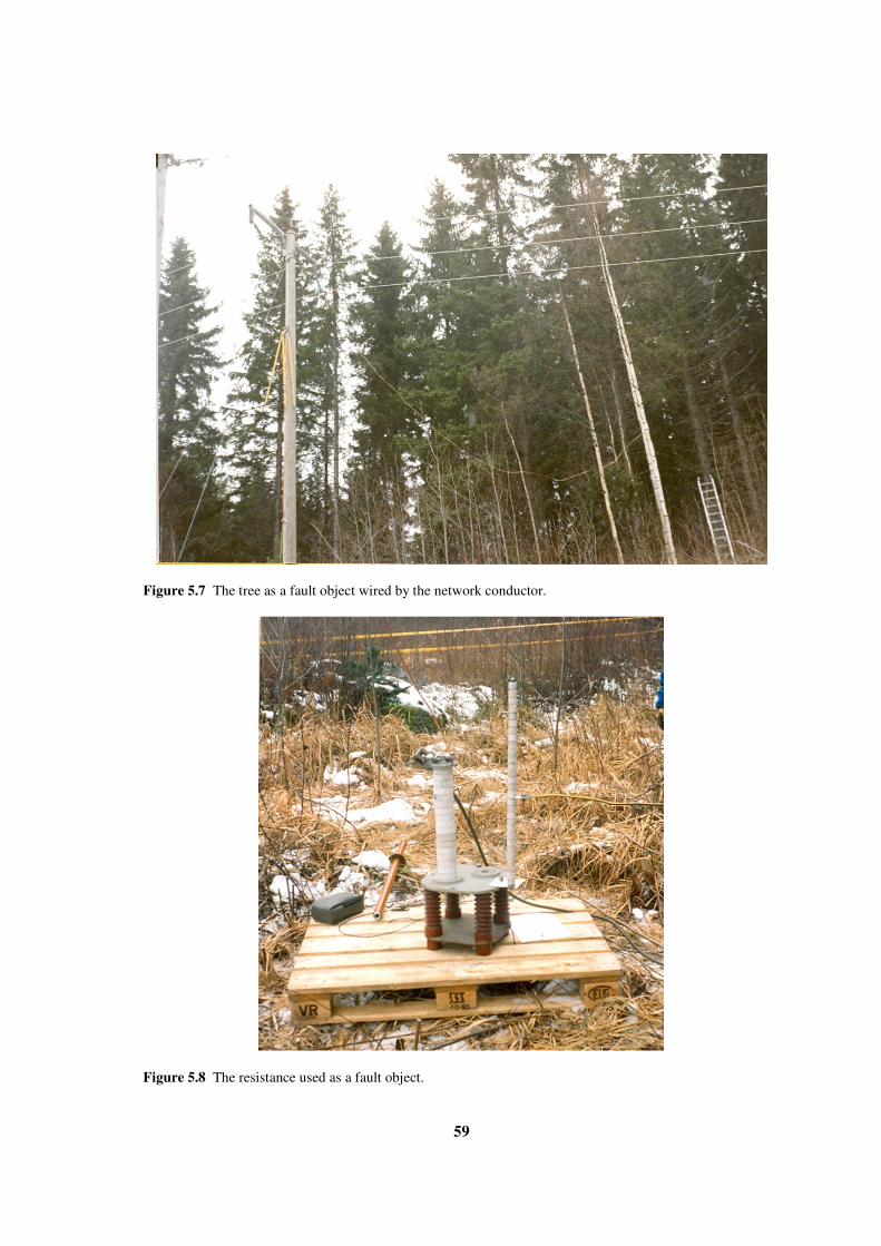
59

Figure 5.7 The tree as a fault object wired by the network conductor.

Figure 5.8 The resistance used as a fault object.

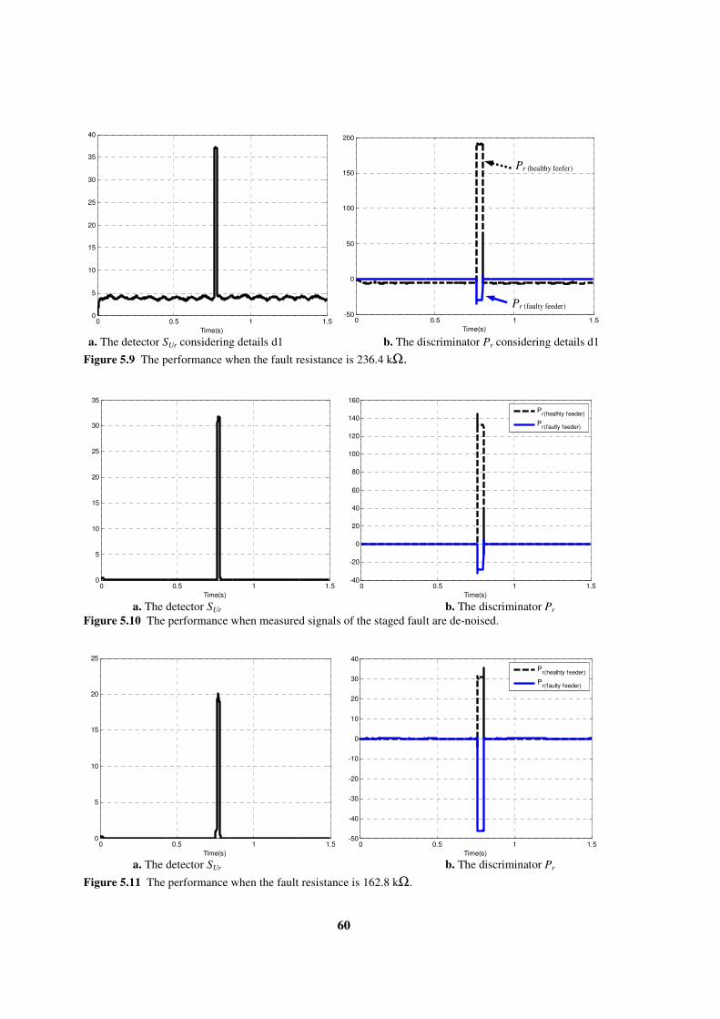
60

0 0.5 1 1.50

5

10

15

20

25

30

35

40

Time(s)

0 0.5 1 1.5-50

0

50

100

150

200

Time(s)

Pr (faulty feeder)

Pr (healthy feefer)

a. The detector SUr considering details d1 b. The discriminator Pr considering details d1

Figure 5.9 The performance when the fault resistance is 236.4 kΩ.

0 0.5 1 1.50

5

10

15

20

25

30

35

Time(s)

0 0.5 1 1.5

-40

-20

0

20

40

60

80

100

120

140

160

Time(s)

Pr(healhty feeder)

Pr(faulty feeder)

a. The detector SUr b. The discriminator Pr

Figure 5.10 The performance when measured signals of the staged fault are de-noised.

0 0.5 1 1.50

5

10

15

20

25

Time(s)

0 0.5 1 1.5

-50

-40

-30

-20

-10

0

10

20

30

40

Time(s)

Pr(healhty feeder)

Pr(faulty feeder)

a. The detector SUr b. The discriminator Pr

Figure 5.11 The performance when the fault resistance is 162.8 kΩ.

61

0 0.5 1 1.50

1

2

3

4

5

6

7

8

9

Time(s)

0 0.5 1 1.5-4

-2

0

2

4

6

8

10

Time(s)

Pr(healhty feeder)

Pr(faulty feeder)

a. The detector SUr b. The discriminator Pr

Figure 5.12 The performance when the fault resistance is 81.7 kΩ.

0 0.5 1 1.50

5

10

15

20

25

30

35

40

Time(s)

0 0.5 1 1.5-20

-10

0

10

20

30

40

50

60

70

80

Time(s)

Pr(healhty feeder)

Pr(faulty feeder)

a. The detector SUr b. The discriminator Pr

Figure 5.13 The performance when the fault resistance is 64 kΩ.

0 0.5 1 1.50

1

2

3

4

5

6

Time(s)

0 0.5 1 1.5

-4

-2

0

2

4

6

8

Time(s)

Pr(healhty feeder)

Pr(faulty feeder)

a. The detector SUr b. The discriminator Pr

Figure 5.14 The performance for a staged fault connected through a tree.

62

0 0.5 1 1.50

2

4

6

8

10

12

14

16

18

Time(s)

0 0.5 1 1.5

-10

0

10

20

30

40

50

60

70

80

Time(s)

Pr(healhty feeder)

Pr(faulty feeder)

a. The detector SUr b. The discriminator Pr

Figure 5.15 The performance for a staged fault connected through a second tree.

0 0.5 1 1.50

5

10

15

20

25

30

35

40

45

Time(s)

0 0.5 1 1.5

-100

-50

0

50

100

150

Time(s)

Pr(healhty feeder)

Pr(faulty feeder)

a. The detector SUr b. The discriminator Pr

Figure 5.16 The performance for a staged fault connected through a third tree.

Table 5.1 The detector S performance for the other staged fault cases.

No. Fault Resistance The detector SUr No. Fault Resistance The detector SUr

1 23.2 kΩ 6.47 6 104.8 kΩ 10.0

2 23.2 kΩ 13.4 7 186.0 kΩ 20.0

3 40.8 kΩ 61.0 8 Tree 45.5

4 40.8 kΩ 6.37 9 Tree 11.1

5 64.0 kΩ 8.59 10 Tree 2.86

63

5.4 Testing the Proposed Detection Technique throughout the Network

[P.VI]

In this section, the proposed detection technique is more tested throughout the network

shown in Figure 4.8. Considering a fault test case occurring at the end of section BD, the

detectors SUr performance for different residual voltages is shown in Figure 5.17. The

detectors respond to the fault disturbance all over the network, which confirms the decision.

The discriminator Pr performance is depicted in Figure 5.18 at the measuring nodes A

and B. At node A, the discriminator polarity is positive for healthy feeders and negative for

the faulty Feeder 1 as shown in Figure 5.18.a. At node B, the discriminator Pr polarity is

positive for the healthy sections BC and BE but it is negative for the faulty section BD

shown in Figure 5.18.b. When the discriminator polarities are checked at the measuring

nodes D and E, they are found positive, ensuring the sections behind are healthy. From the

performance of the discriminator Pr, it can be indicated that the fault is in section BD. The

other fault case occurred at the end of section EF is discussed in [P.VI].

0 0.02 0.04 0.06 0.08 0.1 0.12 0.14 0.160

5

10

15

20

25

30

35

40

Time(s)

SUr(E)

SUr(B)

SUr(A)

SUr(D)

Figure 5.17 The detector SUr using the voltage details when the fault occurred in section BD.

64

0 0.02 0.04 0.06 0.08 0.1 0.12 0.14 0.16-8

-7

-6

-5

-4

-3

-2

-1

0

1

2x 10

-3

Time(s)

Pr of Feeder 1

Pr of the other healthy Feeders

a. The discriminator Pr at node A.

0 0.02 0.04 0.06 0.08 0.1 0.12 0.14 0.16-0.02

-0.015

-0.01

-0.005

0

0.005

0.01

Time(s)

Pr of section BE

Pr of section BC

Pr of section BD

b. The discriminator Pr at node B.

Figure 5.18 The discriminator Pr when the fault occurred in section BD.

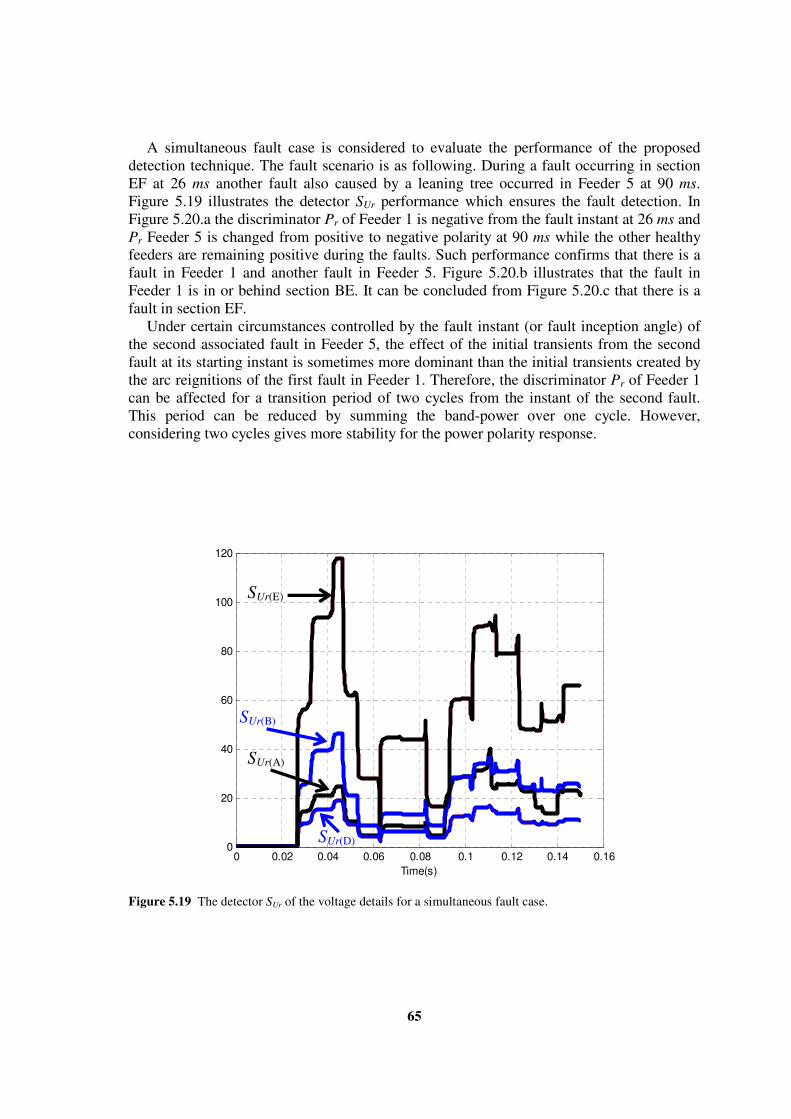
65

A simultaneous fault case is considered to evaluate the performance of the proposed

detection technique. The fault scenario is as following. During a fault occurring in section

EF at 26 ms another fault also caused by a leaning tree occurred in Feeder 5 at 90 ms.

Figure 5.19 illustrates the detector SUr performance which ensures the fault detection. In

Figure 5.20.a the discriminator Pr of Feeder 1 is negative from the fault instant at 26 ms and

Pr Feeder 5 is changed from positive to negative polarity at 90 ms while the other healthy

feeders are remaining positive during the faults. Such performance confirms that there is a

fault in Feeder 1 and another fault in Feeder 5. Figure 5.20.b illustrates that the fault in

Feeder 1 is in or behind section BE. It can be concluded from Figure 5.20.c that there is a

fault in section EF.

Under certain circumstances controlled by the fault instant (or fault inception angle) of

the second associated fault in Feeder 5, the effect of the initial transients from the second

fault at its starting instant is sometimes more dominant than the initial transients created by

the arc reignitions of the first fault in Feeder 1. Therefore, the discriminator Pr of Feeder 1

can be affected for a transition period of two cycles from the instant of the second fault.

This period can be reduced by summing the band-power over one cycle. However,

considering two cycles gives more stability for the power polarity response.

0 0.02 0.04 0.06 0.08 0.1 0.12 0.14 0.160

20

40

60

80

100

120

Time(s)

SUr(A)

SUr(B)

SUr(D)

SUr(E)

Figure 5.19 The detector SUr of the voltage details for a simultaneous fault case.

66

0 0.02 0.04 0.06 0.08 0.1 0.12 0.14 0.16-0.12

-0.1

-0.08

-0.06

-0.04

-0.02

0

0.02

0.04

0.06

Time(s)

Pr of

the faulty Feeder 1

Pr of a healthy Feeder

Pr of the faulty Feeder 5

changed from +ve to -ve

a. At node A.

0 0.02 0.04 0.06 0.08 0.1 0.12 0.14 0.16-0.2

-0.15

-0.1

-0.05

0

0.05

0.1

0.15

Time(s)

Pr of section BE

Pr of section BC

Pr of section BD

b- At node B.

0 0.02 0.04 0.06 0.08 0.1 0.12 0.14 0.16-0.8

-0.6

-0.4

-0.2

0

0.2

0.4

0.6

0.8

Time(s)

Pr of section EF

Pr of section EK

c- At node E.

Figure 5.20 The discriminator Pr behavior during a simultaneous fault case.

67

6- Conclusions and Future Work

6.1 Conclusions

A universal arc representation has been introduced using Modified Mayr (P-τ model) as

an example, in which, the arc equations were solved in the TACS field of the EMTP

program and represented in the power network by TACS controlled voltage source. The arc

voltage and current signals have been measured from the power network into the TACS

field using sensors type 90 and 91, respectively. They have been used as inputs to the

dynamic arc equations. The model parameters have been computed exploiting the

flexibility of FORTRAN expressions in the TACS field. SF6 breakers with experimentally

defined arc parameters have been considered to perform a comparison between the

proposed arc representation and the EMTP built-in model. The thermal limiting curve has

been computed by the proposed and built-in models and compared with the measured

characteristic. Such comparison has confirmed the accuracy of proposed arc representation.

Also, the universality of proposed arc representation has been verified via carrying out

different arc model examples of circuit breaker and transmission line arcing faults. The

study results validated the proposed representation regarding accuracy and universality.

A model for high impedance arcing faults due to leaning trees in MV networks have

been proposed and experimentally verified. The fault was represented in two series parts;

an arc model and a high resistance. The arcing element has been dynamically simulated

using thermal equations. The arc model parameters and resistance values were determined

using the experimental results, where for representing short length and small current arcs,

the parameters have been changed to fit the new application. The fault behavior has been

simulated by the ATP/EMTP program, in which the arc model has been realized using the

universal arc representation.

The electromagnetic transients due to the earth fault caused by tree leaning in MV

networks were discussed where the fault model was incorporated in a 20 kV distribution

network at different locations using ATP/EMTP program. The residual voltage and current

associated with this disturbance have been measured considering different neutral earthing

methods. The main found features of this fault type that can enhance its detection were the

electromagnetic transients created by the periodic arc-reignitions.

Features of earth faults due to leaning trees have been extracted from phase currents

using DWT. Due to the periodicity of arc reignitions, the initial transients have been

localized not only at the fault occurrence instant but also during the fault period that

enhanced the detection security. The absolute sum of the DWT detail d3 coefficient has

been computed over one power cycle for each phase current of each feeder. The faulty

phase had the highest absolute sum when it has been compared with the other healthy

phases. Similarly, the absolute sum of the faulty feeder has been the highest when the

comparison was carried out with respect to other feeders. Therefore, two Logic Functions

have been suggested to determine the faulty phase and faulty feeder.

68

The study has been extended to extract the fault features from residual currents

throughout the network. The DWT performance at different measuring nodes has been

gathered at the base station using wireless sensors concept. Therefore, the DWT has been

evaluated for a wide area of the network and the fault detection has been confirmed by

numerous DWT extractors. In this case, the term of locating the faulty section has been

changed to be based on ratios of the residual current amplitudes.

The other selectivity term of the faulty feeder has been introduced based on a novel

technique by extracting and examining the power polarity. This power is mathematically

processed by multiplying the DWT detail coefficients of the phase voltage and current for

each feeder. Its polarity has discriminated the faulty feeder, in which, the polarity has been

positive when the feeder was healthy and it has been negative when the feeder was faulty.

Such feature has confirmed when considered with any phase. In order to reduce the

computational burden of the technique, the extraction of the fault features was examined

using the residual components instead of the phase components. The same methodology of

computing power has been considered with taking into considerations the residual voltage

and current detail coefficients where the proposed algorithm performance became better.

This proposed algorithm performance has been evaluated using staged fault data. However,

the fault feature was only localized at the fault instant because there was no associated arc

and therefore the transients were not repeated. When the signals have been de-noised, the

detection performance has been improved. Then, this proposed detection technique has

been processed on the residual voltages and currents at different measuring nodes

throughout the network using the distributed wireless sensors and more precise faulty

section discriminator has been attained.

6.2 Future Work

The following points of interest will be extended in work to follow:

1- The high impedance fault modeling issue is required to be extended to cover other

faults such as incipient faults, different fault objects and downed conductor over

different soils. That is because this work only models high impedance faults due to

leaning trees.

2- More scrutiny on the proposed algorithms using staged fault data of the earth faults

due to leaning trees. That is because the performance of the proposed detection

technique is examined using a limited staged fault cases. Extended staged faults are

to be captured with actual fault scenario of leaning trees.

3- Testing probabilistic techniques after extracting the fault features using DWT which

can contribute to more selectivity functions of the fault detection.

69

References

[1] J. Bickford and A. Heaton “Transients Overvoltages on Power Systems”, IEE

Proceeding, Vol. 133, No. 4, pp. 201-225, May 1986.

[2] G. Andersson, P. Donalek, R. Farmer, N. Hatziargyriou, I. Kamwa, P. Kundur, N.

Martins, J. Paserba, P. Pourbeik, J. Sanchez-Gasca, R. Schulz, A. Stankovic, C. Taylor

and V. Vittal "Causes of the 2003 Major Grid Blackouts in North America and Europe

and Recommended Means to Improve System Dynamic Performance" IEEE

Transactions on Power delivery, vol. 20, no. 4, pp. 1922-1928, November 2005.

[3] Report of PSRC Working Group D15 “High Impedance Fault Detection Technology”

March 1996.

[4] Electric Power Research Institute (EPRI), Inc. and EMTP Development Coordination

Group (DCG), Electromagnetic transient programs (EMTP96) rule book, ver 2.0

released on August 1986, and updated ver 3.x on June 1999.

[5] V. Phaniraj and A. Phadke "Modelling of Circuit Breakers in the Electromagnetic

Transients Program" IEEE Transactions on Power Systems, vol. 3, no. 2, pp. 799 –

805, May 1988.

[6] H. Darwish, M. Izzularab and N. Elkalashy “Implementation of Circuit Breaker Arc

Model Using Electromagnetic Transient Program” Middle-East Power Systems

Conference, MEPCON, Hellwan University, Egypt, pp. 809-814, December 2001.

[7] B. Aucoin and R. Jones “High Impedance Detection Implementation Issues” IEEE

Transactions on Power Delivery, vol. 11, no. 1, pp. 139148-594, January 1996.

[8] N. Bhatt "August 14, 2003 U.S.-Canada Blackout" IEEE/PES General Meeting

Denver, USA, June 2004.

[9] U.S-Canada Power System Outage Task Force. (2004) Final Report on the August 14,

2003 Blackout in the United Sates and Canada: Causes and Recommendations.

[Online]. Available: http://www.nerc.com.

[10] S. Larsson and E. Ek "The Blackout in Southern Sweden and Eastern Denmark,

September 23, 2003" IEEE/PES General Meeting, Denver, USA, June 2004.

[11] S. Corsi and C. Sabelli "General Blackout in Italy Sunday September 28th

, 2003, h

03:28:00" IEEE/PES General Meeting, Denver, USA, June 2004.

[12] A. Berizzi, “The Italian 2003 blackout,” in Proc. IEEE/PES General Meeting, Denver,

USA, June 2004.

[13] “Final Report of the Investigation Committee on the 28 September 2003 Blackout in

Italy,” UCTE, 2004.

[14] S. Hänninen , M. Lehtonen, and T. Hakola “Earth Faults and Related Disturbances in

Distribution Networks” IEE Proceedings-Generation, Transmission and Distribution,

Vol. 149, No. 3, pp. 283 – 288, May 2002.

70

[15] S. Hänninen "Single Phase Earth Faults in High Impedance Ground Networks

Characteristics, Indication and Location" Technical Research Centre of Finland

(VTT), Espoo, Finland, 2001.

[16] A. Girgis and F. Ham “A Qualitative Study of Pitfalls in FFT” IEEE Transactions on

Aerospace and Electronic Systems, vol. AES 16, no. 4, pp. 434-439, July 1980.

[17] C. Moo, Y. Chang and P. Mok “A Digital Scheme for Time-Varying Transient

Harmonics” IEEE Transactions on Power Delivery, vol. 10, no. 2, pp. 588-594, April

1995.

[18] Y. Chang, Y. Hsieh and C. Moo "Truncation effects of FFT on estimation of dynamic

harmonics in power system" International Conference on Power System Technology,

PowerCon 2000, Australia, vol. 3, pp. 1155 – 1160, December 2000.

[19] I. Daubechies “Ten Lectures on Wavelets” Regional Conference Series in Applied

Mathematics, the society for Industrial and Applied mathematics, second printing,

1992.

[20] C. Kim and R. Aggarwal “Wavelet Transforms in Power Systems. Part 1 General

Introduction to the Wavelet Transforms” Power Engineering Journal, vol. 14, no. 2,

pp. 81-87, April 2000.

[21] M. Solanki, Y. Song, S. Potts and A. Perks "Transient protection of transmission line

using wavelet transform" IEE 7th

International Conference on Developments in Power

System Protection, pp. 299–302, 9-12 April 2001.

[22] H. Darwish, M. Farouk, A. Taalab, N. Mansour "Investigation of Real–Time

Implementation of DSP-Based DWT for Power System Protection” IEEE/PES

Transmission and Distribution Conference and Exposition, Dallas, Texas, USA, May

2006.

[23] T. Zheng and E. Makram “An Adaptive Arc Furnace Model” IEEE Transactions on

Power Delivery, Vol. 15, No. 3, pp 931-939, July 2000.

[24] M. Aucoin, B. Russell and C. Benner “High Impedance Fault Detection for Industrial

Power Systems” Conference Record of the 1989 IEEE Industry Applications Society

Annual Meeting, October 1989.

[25] V. Terzija, N. Elkalashy, G. Preston, V. Stanojević, G. Štrbac "Detection of Arcing

Faults: Modelling, Simulation, Testing and Algorithms Aspects" PowerTech 2007,

Lausanne, Switzerland, July 2007.

[26] N. Elkalashy, H. Darwish, A. Taalab, and M. Izzularab, "An Adaptive Single Pole

Autoreclosure Based on Zero Sequence Power" Electric Power Systems Research,

Vol. 77, No. 5-6, pp. 438-446, April 2007.

[27] R. Aggarwal, A. Johns, Y. Song, R. Dunn, and D. Fitton “Neural-Network Based

Adaptive Single-Pole Aotureclosure Technique for EHV Transmission Systems,” IEE

Proceedings-Generation, Transmission and Distribution, Vol. 141, No. 2, pp. 155-

160, March 1994.

[28] H. Darwish, M. Izzularab, and N. Elkalashy “Enhanced Commutation Circuit Design

of HVDC Circuit Breaker Using EMTP”, IEEE/PES, Transmission and distribution,

TD 2005/2006, pp 978 – 985, USA, 21-24 May 2006.

71

[29] H. Darwish, M. Izzularab, and N. Elkalashy, "Real-time testing of hvdc circuit

breakers" the 14th International Conference on power System Protection, PSP2004,

Bled, Slovenia, 2004.

[30] J. Blackburn Protective Relaying. Principles and applications, second edition, Marcel

Dekker, Inc, New Yourk, 1998.

[31] C.K. Wong, C.W. Lam, K.C. Lei, C.S. Lei, and Y.D. Han ”Novel Wavelet Approach

to Current Differential Pilot Relay Protection,” IEEE Transactions on Power Delivery,

Vol. 18, No. 1, pp 20-25, January 2003.

[32] H. Darwish, A-M. Taalab, A. Osman, N. Mansour and O. Malik "Experimental

Evaluation of DWT-Based Current Spike Comparator for Line Protection" IEEE/PES

Power Systems Conference and Exposition, PSCE '06, pp. 1371 – 1379, 2006.

[33] H. Darwish, A-M. Taalab and E. Ahmed “Investigation of power differential concept

for line protection” IEEE Transactions on Power Delivery, Vol. 20, No. 2, pp 617-

621, April 2005.

[34] A-M. Taalab, H. Darwish and E. Ahmed “Performance of Power Differential Relay

with Adaptive Setting for Line Protection” IEEE Transactions on Power Delivery,

Vol. 22, No. 1, pp 50-58, January 2007.

[35] A. Pradhan, A. Routray and S. Gudipalli “Fault Direction Estimation in Radial

Distribution System Using Phase Change in Sequence Current” IEEE Transactions on

Power Delivery, Vol. 22, No. 4, October 2007.

[36] M. Lehtonen and T. Hakola “Neutral Earthing and Power System Protection. Earthing

Solutions and Protective Relaying in Medium Voltage Distribution Networks”, ABB

Transmit Oy, FIN-65101 Vassa, Finland, 1996.

[37] G. Benner and B. Russell "Practical High-Impedance Fault Detection on Distribution

Feeders" IEEE Transactions on Industry Applications, Vol. 33, No. 3, pp. 635-640,

May/June 1997.

[38] A. Girgis, W. Chang and E. Makram “Analysis of high-impedance fault generated

signals using a Kalman filtering approach”, IEEE Transactions on Power delivery,

Vol. 5, No. 5, pp. 1714-1724, October 1990.

[39] A. Mamishev, B. Russell and G. Benner “Analysis of High Impedance Faults Using

Fractal Techniques”, IEEE Transactions on Power delivery, Vol. 11, No. 1, pp. 435-

440, February 1996.

[40] A. Sedighi, M. Haghifam, O. Malik and M. Ghassemian "High Impedance Fault

Detection Based on Wavelet Transform and Statistical Pattern Recognition" IEEE

Transaction on Power delivery, Vol. 20, No. 4, pp. 1414-2421, October 2005.

[41] M. Michalik, W. Rebizant, M. Lukowicz, S. Lee and S. Kang "High-impedance fault

detection in distribution networks with use of wavelet-based algorithm" IEEE

Transactions on Power Delivery, vol. 21, no. 4, pp. 1793 – 1802, October 2006.

[42] C. Kim, H. Kim, Y. Ko, S. Byun, K. Aggarwal and A. Johns "A novel fault-detection

technique of high-impedance arcing faults in transmission lines using the wavelet

transform" IEEE Transactions on Power delivery, Vol. 17, No. 4, pp. 921-929,

October 2002.

72

[43] D. Wai and X. Yibin “A Novel Technique for High Impedance Fault Identification”,

IEEE Transactions on Power delivery, Vol. 13, No. 3, pp. 738-744, July 1998.

[44] B. Russell and C. Benner "Arcing Fault Detection for Distribution Feeders: Security

Assessment in Long Term Field Trials", IEEE Transactions on Power delivery, Vol.

10, No. 2, pp. 676-683, April 1995.

[45] D. Jeeringes and J. Linders “Unique Aspects of Distribution System Harmonics due to

High Impedance Ground Faults”, IEEE Transactions on Power delivery, Vol. 5, No. 2,

pp. 1086-1094, April 1990.

[46] T. Grima and J. Flatermeier "A New Generation of Materials for Medium Voltage

Compensated Neutral Networks" IEE 14th

International Conference and Exhibition on

Electricity Distribution, CIRED, Birmingham, 2-5 June 1997.

[47] G. Druml, A. Kugi and O. Seifert "A New Directional Transient Relay for High

Ohmic Earth Faults" IEE 17th

International Conference and Exhibition on Electricity

Distribution, CIRED, Bercelona, 12-15 May 2003.

[48] Y. Assef, P. Bastard and M. Meunier "Artificial Neural Networks for Single Phase

Fault Detection in Resonant Grounded Power Distribution Systems" IEEE

Transmission and Distribution Conference, Los Angeles, September 1996.

[49] A. Sultan, G. Swift and D. Fedirchuk “Detecting Arcing Downed-Wires Using Current

Flicker and Half-Cycle Asymmetry” IEEE Transactions on Power Delivery, Vol. 9,

No. 1, pp 461-467, January 1994.

[50] V. Leitloff, R. Feuillet and D. Griffel "Detection of Resistive Single-Phase Earth

Faults in a Compensated Power-Distribution System" European Transactions on

Electrical Power System, ETEP, Vol. 7, No. 1, pp. 65- 73, January 1997.

[51] S. Santoso, E. Powers, W. Grady and P. Hofmann “Power quality assessment via

wavelet transform analysis” IEEE Transactions on Power Delivery, vol. 11, no. 2, pp.

924 – 930, April 1996.

[52] P. Dash, B. Panigrahi, D. Sahoo and G. Panda “Power quality disturbance data

compression, detection, and classification using integrated spline wavelet and S-

transform” IEEE Transactions on Power Delivery, vol. 18, no. 2, pp. 595 – 600,

April 2003

[53] C. Lin and C. Wang “Adaptive wavelet networks for power-quality detection and

discrimination in a power system” IEEE Transactions on Power Delivery, vol. 21, no.

3, pp. 1106 – 1113, July 2006.

[54] S. Santoso, W. Grady, E. Powers, J. Lamoree and S. Bhatt “Characterization of

distribution power quality events with Fourier and wavelet transforms” IEEE

Transactions on Power Delivery, vol. 15, no. 1, pp. 247 – 254, January 2000.

[55] L. Tao, M. Tsuji and E. Yamada “Wavelet approach to power quality monitoring” The

27th

Annual Conference of the IEEE Industrial Electronics Society, IECON '01, pp.

670 – 675, 2001.

[56] C. Kim, S. Park, R. Aggarwal and A. Johns “A noise suppression method for

improvement of power quality using wavelet transforms” IEEE Power Engineering

Society Summer Meeting, pp. 414 – 419, July 1999.

73

[57] M. Florkowski “Wavelet based partial discharge image de-noising” 11th

International

Symposium on High Voltage Engineering, pp. 21 – 24, August 1999.

[58] G. Hashmi, M. Lehtonen, R. Jabbar and S. Qureshi “Wavelet-based De-noising of

Partial Discharge Signals in MV Covered-Conductor Networks" Australasian

Universities Power Engineering Conference, AUPEC2006, Victoria, Australia,

December 2006.

[59] W. Xiaorong, G. Zongjun, S. Yong and Y. Zhang “Extraction of partial discharge

pulse via wavelet shrinkage” 6th International Conference on Properties and

Applications of Dielectric Materials, Volume 2, pp. 685 – 688, June 2000.

[60] H. Zhang,T. Blackburn, B. Phung and D. Sen; “A novel wavelet transform technique

for on-line partial discharge measurements. 1. WT de-noising algorithm” IEEE

Transactions on Dielectrics and Electrical Insulation, vol 14, no. 1, pp. February

2007

[61] M. Hu; X. Jiang; H. Xie; Z. Wang; “A new technique for extracting partial discharge

signals in on-line monitoring with wavelet analysis” International Symposium on

Electrical Insulating Materials, pp.677 – 680, September 1998.

[62] O. Youssef "Applications of fuzzy-logic-wavelet-based techniques for transformers

inrush currents identification and power systems faults classification" IEEE PES

Power Systems Conference and Exposition, pp. 553 – 559, October 2004.

[63] O. Youssef "A wavelet-based technique for discrimination between faults and

magnetizing inrush currents in transformers" IEEE Transactions on Power Delivery,

vol. 18, no. 1, pp. 170 – 176, January 2003.

[64] H. Mortazavi, H. Khorashadi-Zadeh "A new inrush restraint algorithm for transformer

differential relays using wavelet transform" International Conference on Power System

Technology, PowerCon2004, vol. 2, pp. 1705 – 1709, November 2004

[65] K. Bulter-Purry and M. Bagriyanik "Characterization of Transients in Transformers

Using Discrete Wavelet Transforms" IEEE Transactions on Power Systems, vol. 18,

no. 2, pp. 648-656, May 2003.

[66] J. Faiz, S . Lotfi-Fard "A novel wavelet-based algorithm for discrimination of internal

faults from magnetizing inrush currents in power transformers" IEEE Transactions on

Power Systems, vol. 21, no. 4, pp. 1989- 1996, October 2006.

[67] C. Aguilera, E. Orduna and G. Ratta " Fault detection, classification and faulted phase

selection approach based on high-frequency voltage signals applied to a series-

compensated line" IEE Proceedings on Generation, Transmission and Distribution,

vol. 153, no. 4, pp. 469 – 475, July 2006.

[68] H. Darwish, A-M. Taalab, A. Osman, N. Mansour and O. Malik "Spectral Energy

Differential Approach for Transmission Line Protection" IEEE/PES Power Systems

Conference and Exposition, PSCE '06, pp. 1931 – 1937, 2006.

[69] A. Osman, O. Malik "Transmission line distance protection based on wavelet

transform" IEEE Transactions on Power Delivery, vol. 19, no. 2, pp. 515 – 523, April

2004.

74

[70] S. Saleem and A. Sharaf "Ultra High Speed Protection of Series Compensated

Transmission Lines using Wavelet Transforms" Canadian Conference on Electrical

and Computer Engineering, pp. 1130 – 1134, May 2006.

[71] A. Osman, O. Malik "Protection of parallel transmission lines using wavelet

transform" IEEE Transactions on Power Delivery, vol. 19, no. 1, pp. 49 – 55, January

2004.

[72] O. Youssef "Online Applications of Wavelet Transforms to Power System Relaying"

IEEE Transactions on Power Delivery, vol. 18, no. 4, pp. 1158 – 1165, October

2003.

[73] H. Mokhtari and R. Aghatehrani "A new Wavelet-Based Method for Detection of

High Impedance Faults" International Conference on Future Power Systems,

November 2005.

[74] D. Wai, X. Yibin "A novel technique for high impedance fault identification" IEEE

Transactions on Power Delivery, vol. 13, no. 3, pp. 738 – 744, July 1998.

[75] S. Huang, C. Hsieh "High-impedance fault detection utilizing a Morlet wavelet

transform approach" IEEE Transactions on Power Delivery, vol. 14, no. 4, pp. 1401

– 1410, October 1999.

[76] K. Silva, B. Souza, N. Brito "Fault detection and classification in transmission lines

based on wavelet transform and ANN" IEEE Transactions on Power Delivery, vol. 21,

no. 4, pp. 2058- 2063, October 2006.

[77] Z. Huang, Y. Chen and Q. Gong "A protection and fault location scheme for EHV line

with series capacitor based on travelling waves and wavelet analysis" International

Conference on Power System Technology, PowerCon 2002, vol. 1, pp. 290 – 294,

October 2002.

[78] A. Ametani “Power System Transient Analysis by EMTP” Middle-East Power

Systems Conference, MEPCON, Hellwan University, Egypt, pp. 1-12, December 2001.

[79] I. Marti and L. Linares “Real-Time EMTP-Based Transients Simulation” IEEE

Transaction on Power Systems, Vol. 9, No. 3, P. 1309-1317, August 1994.

[80] R. Lasseter, K. Fehrle and B. Lee Electromagnetic Transient Program (EMTP),

Workbook IV (TACS). El-4651, EPRI Research Project 2140-6, Palo Alto, CA 94303,

June 1989.

[81] L. Prikler and H. Hoildalen ATPDraw Users Manual, SINTEF Energy Research AS,

Norway, TR F5680, ISBN 82-594-2344-8, August 2002.

[82] E. Shade and K. Ragaller “Dielectric Recovery of an Axially Blown SF6 Arc after

Current Zero: Part I – Experimental Investigations” IEEE Transactions on Plasma

Science, Vol. PS-10, No. 3, P. 141-153, September 1982.

[83] K. Ragaller, W. Egli and K. Brand “Dielectric Recovery of an Axially Blown SF6 Arc

after Current Zero: Part II – Theoretical Investigations” IEEE Transactions on Plasma

Science, Vol. PS-10, No. 3, P. 154-162, September 1982.

[84] K. Brand, W. Egli, L. Niemeyer, K. Ragaller and E. Shade “Dielectric Recovery of an

Axially Blown SF6 Arc after Current Zero: Part III– Comparison of Experimental and

Theoretical” IEEE Transactions on Plasma Science, Vol. PS-10, No. 3, P. 162-172,

September 1982.

75

[85] H. Schoetzau, H. Meili, E. Fischer, C. Strurzenegger and H. Graf “Dielectric Phase in

an SF6 Breaker” IEEE Transactions on Power Apparatus and System, Vol. Pas-104,

No. 7, P. 1897-1902, July/August 1985.

[86] T. Browne “A Study of AC Arc Behavior Near Current Zero by Means of

Mathematical Models” AIEE, Vol. 67, P. 141-153, 1948.

[87] P. Scarpa, B. Dauby, J. Defise, W. Legros, M. Barrault, G. Bernard and S. Rowe “SF6

Auto-Expansion Circuit Breaker Design: Numerical and Experimental Investigations

of Arc-Gas Interactions” IEEE Transactions on Power Delivery, Vol. 7, No. 1, P. 339-

345, January 1992.

[88] A. Cassie “Theorie Nouvelle des Arcs de Rupture et de la Rigidité des Circuits” Cigre

Report 102, pp. 588-608, 1939.

[89] O. Mayr “Beitrage zur Theorie des Statischen und des Dynamischen Lichthogens”

Archiv für Elektrotechnik, Vol. Band 37, No. Heft 12, pp. 588-608, 1943.

[90] W. Hermann, U. Kogelschatz, L. Niemeyer, K. Ragaller and E. Schade “Investigation

on the Physical Phenomena around Zero in HV Gas Blast Breakers” IEEE

Transactions on Power Apparatus and System, Vol. PAS-95, No. 4, July/August 1976.

[91] K. Ragaller, A. Plessel, W. Herman and W. Egli “Calculation Methods for the ARC

Quenching System of Gas Circuit Breaker” CIGRE-13.03, Paris, France, 1984.

[92] Cigre Working Group 13.01 “Applications of Black Box Modeling to Circuit

Breakers” Electra, No. 149, August 1993.

[93] T. Brwone “Practical Modeling of the Circuit Breaker Arc as a Short Line Fault

Interrupter” IEEE Transactions on Power Apparatus and System, Vol. PAS-97, No. 3,

P. 838-845, May/June 1978.

[94] U. Habedank “Application of a New Arc Model for the Evaluation of Short-Circuit

Breaking Tests” IEEE Transactions on Power Delivery, Vol. 8, No. 4, P. 1921-1925,

October 1993.

[95] P. Schavemaker and L. Sluis “An Improved Mayr-Type Arc Model Based on Current-

Zero Measurements” IEEE Transactions on Power Delivery, Vol. 15, No. 2, P. 580-

584, April 2000.

[96] L. Frost “Dynamic Arc Analysis of Short Line Fault Tests for Accurate Circuit

Breaker Performance Specification” IEEE Transactions on Power Apparatus and

System, Vol. PAS-97, No. 2, P. 478-484, March/April 1978.

[97] U. Habedank and H. Knobloch “Zero-Crossing Measurements as a Tool in the

Development of High-Voltage Circuit Breakers” IEE Proceedings-Science

Measurement and Technology, Vol. 148, No. 6, November 2001

[98] M. Hrabovsky, V. Mastny and Z. Vostracky “Application of Mathematical Arc Model

for Determination of Thermal Failure Limiting Characteristics” CIGRE, 1984.

[99] K. Cornick, Y. Ko and B. Pek “Power System Transients Caused by Arcing Faults”

IEE Proceedings, Vol. 128, No. 1, pp. 18-27, January 1981.

[100] M. Kizilcay and T. Pniok “Digital Simulation of Fault Arcs in Power systems”

European Transactions on Electrical Power System, ETEP, Vol. 4, No. 3, pp. 55-59,

January/February 1991.

76

[101] M. Kizilcay and K. Koch "Numerical Fault Arc Simulation Based on Power Arc

Tests" European Transactions on Electric Power, ETEP, vol. 4, no. 3, pp. 177-186,

May/June 1994.

[102] A. Johns, R. Aggarwal and Y. Song “Improved Techniques for Modeling Fault Arcs

on Faulted EHV Transmission Systems” IEE Proceedings-Generation, Transmission

and Distribution, Vol. 141, No. 2, pp. 148-154, March 1994.

[103] J. Sousa, D. Santos and M. Barros “Fault Arc Modeling in EMTP” International

Power System Transient Conference, IPST’95, Lisbon, pp. 475-480, September 1995.

[104] V. Terzija and H. Koglin “Long Arc in Free Air: Laboratory Testing, Modeling,

Simulation and Model-Parameters Estimation” IEE Proceedings-Generation,

Transmission and Distribution, Vol. 49, No. 3, pp. 319-325, May 2002.

[105] Y. Goda, M. Iwata, K. Ikeda and S. Tanaka “Arc Voltage Characteristics of high

Current Fault Arcs in Long Gaps” IEEE Transactions on Power Delivery, Vol. 15, No.

2, pp. 791-795, April 2000.

[106] M. Kizilcay and P. Seta "Digital Simulation of Fault Arcs in Medium-Voltage

Distribution Networks" 15th

Power Systems Computation Conference, PSCC, Liege,

Belgium, 22-26 August 2005.

[107] Wavelet Toolbox for MATLAB, Math Works 2005.

[108] J. Haung, C. Shen, S. Phoong and H. Chen "Robust Measure of Image Focus in the

Wavelet Domain" International Symposium on Intelligent Signal Processing and

Communication Systems, ISPACS, Hong Kong, December 2006.

[109] M. Nordman and T. Korhonen “Design of a Concept and a Wireless ASIC Sensor

for Locating Earth Faults in Unearthed Electrical Distribution Networks” IEEE

Transactions on Power delivery, Vol. 21, No. 3, pp. 1074-1082, July 2006.

[110] R. Fernandes “Electrical Power Line and Substation Monitoring apparatus and

systems” European Patent Application 0314849, May 1989.

[111] O. Vähämäki, K. Rautiainen and K. Kauhaniemi “Measurement of Quantities of

Electric Line” Patent Application WO0171367, September 2001.

[112] M. Vieira, C. Coelho, D. da Silva and J. da Mata “Survey on Wireless Sensor

Network Devices” Emerging Technologies and Factory Automation, ETFA'03, pp.

537–544, September 2003.

ISBN 978-951-22-9014-7ISBN 978-951-22-9015-4 (PDF)ISSN 1795-2239ISSN 1795-4584 (PDF)