Modeling and Bayesian parameter estimation for shapememory alloy bending actuators

John H. Crewsa and Ralph C. Smitha

aDepartment of Mathematics, Center for Research in Scientific Computation, North CarolinaState University, Raleigh, NC, United States

ABSTRACT

In this paper, we employ a homogenized energy model (HEM) for shape memory alloy (SMA) bending actuators.Additionally, we utilize a Bayesian method for quantifying parameter uncertainty. The system consists of a SMAwire attached to a flexible beam. As the actuator is heated, the beam bends, providing endoscopic motion. Themodel parameters are fit to experimental data using an ordinary least-squares approach. The uncertainty inthe fit model parameters is then quantified using Markov Chain Monte Carlo (MCMC) methods. The MCMCalgorithm provides bounds on the parameters, which will ultimately be used in robust control algorithms. Onepurpose of the paper is to test the feasibility of the Random Walk Metropolis algorithm, the MCMC methodused here.

Keywords: shape memory alloys, uncertainty quantificiation, markov chain monte carlo

1. INTRODUCTION

Shape memory alloys (SMA) are unique actuators that are gaining increased utilization in prototypes such asrobotic catheters,1,2 robotic hands,3 jet chevrons,4,5 and underwater vessels.6 SMA actuators are capable ofrecovering large strains (approximately 5%) upon heating. However, the control and optimization of SMA devicesis complicated by the material’s nonlinear, hysteretic dependence on stress and temperature.

In this paper we employ a computationally efficient model for a SMA bending actuator. Furthermore,we utilize Markov Chain Monte Carlo (MCMC) methods to quantify parameter uncertainty in a systematicmanner. MCMC methods are based on Bayes’ rule, which relates the posterior density of model parameters toa prior density and the likelihood of those parameters.7,8 MCMC methods avoid the difficulty of calculating thelikelihoods directly (and integrating over the parameter space) by creating a Markov Chain where the stationarydistribution is the posterior distribution. A proposal function and an accept-reject rule determine the randomwalk of the Markov Chain.9 The main goal of this paper is to test the feasibility of the approach for the SMAbending actuator under consideration.

An algorithmic approach to quantifying parametric uncertainty is useful for numerous reasons. The resultscan be used to produce bounds on the model output for comparison to experimental data. An additional use forSMA actuators (in particular the bending actuator under consideration) is to quantify parameter uncertainty forcontrol algorithms. Robust control methods require some measure of model uncertainty in order to guaranteestability or optimality. For example, sliding mode control (or variable structure control) requires bounds onmodel uncertainty in order to ensure the attractiveness of the sliding surface.10

The remainder of this paper is organized as follows. The model of a flexible beam actuated by a single SMAtendon is presented first. The homogenized energy model (HEM) is used, which has been applied to various smartmaterials.11–20 The approach to quantify uncertainty is described, including optimization of model parametersand the Markov Chain Monte Carlo method used here. Finally, the results are presented.

Further author information: (Send correspondence to J. Crews)J. Crews: E-mail: jhcrews@ncsu.edu, Telephone: 1 919 515 0684

2. HOMOGENIZED ENERGY MODEL OF A SINGLE-TENDON SHAPE MEMORYALLOY BENDING ACTUATOR

The system consists of a flexible beam actuated by a single shape memory alloy (SMA) tendon, as depicted inFigure 1(a). The SMA tendon (actuator) is held a fixed distance from the neutral axis of the flexible beam usingrapid-prototyped collets. The SMA actuator is pre-strained before it is attached to the axially stiff, laterallycompliant beam. Therefore, a moment is created as the SMA tendon contracts due to Joule heating and thestructure bends in the manner shown in Figure 1(b). Similar robotic systems include catheters and smartinhalers.21,22 A mesoscopic free energy model of a catheter was introduced in Veeramani et al.,1 with furtherwork in Crews et al.2,23

2.1 System Model

As shown in,2,23 the bending angle θ(t) can be related to the SMA tendon stress σ(t) by the relation

θ(t) =aAcLσ(t)

EI, (1)

where a is the actuator offset from the neutral axis, Ac is the cross-sectional area of the SMA actuator, L isits length, E is the elastic (Young’s) modulus of the flexible beam, and I is its area moment of inertia. Thestress-strain relationship for the bending system can be simplified to

σ(t) =EI

a2Ac(εP − ε(t)) , (2)

where εP is the pre-strain in the SMA actuator. Equation (2) reduces the planar bending problem to a one-dimensional problem consisting of a SMA actuator in parallel with a linear spring with stiffness

K =EI

a2Ac. (3)

The SMA strain ε(t) is modeled using the homogenized energy model. The HEM accounts for materialinhomogeneities and interaction effects to accurately and efficiently quantify the macroscopic SMA behavior.A complete derivation of the model and data-driven techniques for estimating model parameters are providedin.17 In Crews et al.,17 a single SMA actuator in constant-temperature conditions was considered. The relevantrelationships and equations are summarized here in order to tailor the HEM to the bending system underconsideration.

The HEM quantifies the macroscopic strain

ε(t) =

∫ ∞0

∫ ∞−∞

νR(σR)ν(σI)ε (σ(t) + σI , T (t);σR) dσIdσR (4)

(a) (b)

Figure 1: (a) Flexible beam actuated by single SMA tendon; (b) Time-lapse photograph of robotic system.

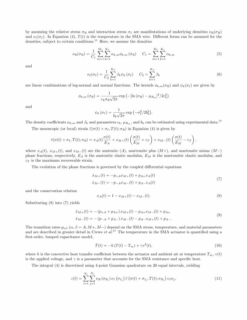
by assuming the relative stress σR and interaction stress σI are manifestations of underlying densities νR(σR)and νI(σI). In Equation (4), T (t) is the temperature in the SMA wire. Different forms can be assumed for thedensities, subject to certain conditions.11 Here, we assume the densities

νR(σR) =1

C1

Mα∑m=1

Kα∑k=1

αk,mφk,m (σR) C1 =

Mα∑m=1

Kα∑k=1

αk,m (5)

and

νI(σI) =1

C2

Kβ∑k=1

βkψk (σI) C2 =

Kβ∑k=1

βk (6)

are linear combinations of log-normal and normal functions. The kernels φk,m(σR) and ψk(σI) are given by

φk,m (σR) =1

ckσR√

2πexp

(−[ln (σR)− µRm ]2/2c2k

)and

ψk (σI) =1

bk√

2πexp

(−σ2

I/2b2k

).

The density coefficients αk,m and βk and parameters ck, µRm , and bk can be estimated using experimental data.17

The mesoscopic (or local) strain ε(σ(t) + σI , T (t);σR) in Equation (4) is given by

ε(σ(t) + σI , T (t);σR) = xA(t)σ(t)

EA+ xM+(t)

(σ(t)

EM+ εT

)+ xM−(t)

(σ(t)

EM− εT

),

where xA(t), xM+(t), and xM−(t) are the austenite (A), martensite plus (M+), and martensite minus (M−)phase fractions, respectively, EA is the austenitic elastic modulus, EM is the martensitic elastic modulus, andεT is the maximum recoverable strain.

The evolution of the phase fractions is governed by the coupled differential equations

xM+(t) = −p+AxM+(t) + pA+xA(t)

xM−(t) = −p−AxM−(t) + pA−xA(t)(7)

and the conservation relationxA(t) = 1− xM+(t)− xM−(t). (8)

Substituting (8) into (7) yields

xM+(t) = − (p+A + pA+)xM+(t)− pA+xM−(t) + pA+

xM−(t) = − (p−A + pA−)xM−(t)− pA−xM+(t) + pA−.(9)

The transition rates pαβ (α, β = A,M+,M−) depend on the SMA stress, temperature, and material parametersand are described in greater detail in Crews et al.17 The temperature in the SMA actuator is quantified using afirst-order, lumped capacitance model,

T (t) = −h (T (t)− T∞) + γv2(t), (10)

where h is the convective heat transfer coefficient between the actuator and ambient air at temperature T∞, v(t)is the applied voltage, and γ is a parameter that accounts for the SMA resistance and specific heat.

The integral (4) is discretized using 4-point Gaussian quadrature on 20 equal intervals, yielding

ε(t) =

Ni∑i=1

Nj∑j=1

νR (σRi) νI(σIj)ε(σ(t) + σIj , T (t);σRi

)viwj , (11)

where σRi and σIj are the quadrature points and vi and wj are the quadrature weights. The summations in (11)can be converted to the vector-matrix-vector product

ε(t) = V TΓW,

whereV T = [v1νR(σR1

), · · · , vNiνR(σRNi )]

WT = [w1νI(σI1), · · · , wNjνI(σINj )]

Γ = XAσ(t)EA

+XM+

(σ(t)EM

+ εT

)+XM−

(σ(t)EM− εT

).

The Ni ×Nj matrices XA, XM+, and XM− evaluate the phase fractions at

[Xα(t, σ(t), T (t))]ij = xα(t, σ(t) + σIj , T (t);σRi

)α = A,M+,M−,

where xα are the solutions to (7) and (8).

The ODEs (9) are discretized and solved using an implicit Euler scheme. For discretized time tk = k∆t,stress σk = σ(tk), and temperature T k = T (tk) values, the implicit Euler discretization yields

ak+111 xk+1

M+ + ak+112 xk+1

M− = xkM+ + ak+113

ak+121 xk+1

M+ + ak+122 xk+1

M− = xkM− + ak+123 ,

(12)

whereak+111 = 1 + ∆t (p+A + pA+) ak+1

21 = pA−∆t

ak+112 = pA+∆t ak+1

22 = 1 + ∆t (p−A + pA−)

ak+113 = pA+∆t ak+1

23 = pA−∆t.

(13)

Note that in (13), the transition rates depend on σk, T k, σI , and σR. The austentic phase fraction xk+1A is given

by the conservation relation (8). The implicit Euler discretization of the temperature yields

T k+1 = dk+11 T k + dk+1

2 ,

where

dk+11 =

1

1 + h∆tdk+12 =

∆t(hT∞ + γ

(vk+1

)2)1 + h∆t

.

The stress σk is found by substituting (11) into (2) and solving for the equilibrium stress, which yields

σk =εP − εT

(V TXM+W − V TXM−W

)a2AcEI + V TXAW

1EA

+ V TXM+W1EM

+ V TXM−W1EM

.

Equation (12) can be solved using Cramer’s rule, which gives

xk+1M+ = ck+1

11 xkM+ + ck+112 xkM− + ck+1

13

xk+1M− = ck+1

21 xkM+ + ck+122 xkM− + ck+1

23 ,

where

ck+111 =

ak+122

det ck+112 = −a

k+112

det ck+113 = 1

det

(ak+122 ak+1

13 − ak+112 ak+1

23

)ck+121 = −a

k+121

det ck+122 =

ak+111

det ck+123 = 1

det

(ak+111 ak+1

23 − ak+113 ak+1

21

)det = ak+1

11 ak+122 − a

k+112 ak+1

21 .

(14)

The computational efficiency of the model can be improved by storing 4-D arrays Pαβ of the transition ratesevaluated at the quadrature points σRi and σIj and uniformly distributed values of the stress σ` and temperatureT m, where σmin ≤ σ` ≤ σmax and Tmin ≤ T m ≤ Tmax. For example,

[P`m+A]ij = p+A(σ` + σIj , T m;σRi

).

During implementation, the indices ` and m corresponding to values nearest to σk and T k are found and theNi×Nj matrices P`mαβ are used to calculate the matrices corresponding to (14), Ck+1

11 , · · · , Ck+123 . These matrices

can be rapidly calculated using point-wise operations. The matrices of the phase fractions can then be updatedin one step using the relations

Xk+1M+ = Ck+1

11 .×XkM+ + Ck+1

13 .×XkM− + Ck+1

13

Xk+1M− = Ck+1

21 .×XkM+ + Ck+1

23 .×XkM− + Ck+1

23

Xk+1A = 1−Xk+1

M+ −Xk+1M−

, (15)

where point-wise multiplication (.×) and summation are again used. In Equation (15), 1 is the Ni×Nj identitymatrix.

3. PARAMETER UNCERTAINTY QUANTIFICATION

Numerous techniques exist to estimate uncertainty in model parameters. Frequentist approaches involve multiplemeasurements or samples of experimental data. However, collecting large sets of data can be expensive and timeconsuming. One method that overcomes these limitations is bootstrapping.24–26 Here, we are testing the Bayesianframework by using Markov Chain Monte Carlo (MCMC) algorithms. First, we determine the optimal modelparameters using standard least-squares approaches. Then, we use the optimization results to determine thecovariance matrix for the MCMC’s proposal function.

3.1 Ordinary Least Squares Fit of Model Parameters

The optimization algorithm minimizes

F (~p) =1

2

N∑i=1

(y(ti)− y(ti; ~p))2, (16)

the sum of squared error between the experimentally measured bending angle y(ti) and the model predictedbending angle y(ti; ~p) = θ(ti; ~p) given by Equation (1). A complete list of the model parameters ~p is provided inTable 1. Here, we are including all the SMA model parameters in the optimization routine. Alternatively, onecould optimize the SMA model parameters (such as αk,m through V in Table 1) using tensile-test data17 andthen only fit the heat transfer and bending model parameters using the measured bending angle. Including allthe parameters will produce a lower sum of squared error but neglects the coupling between parameters.

3.2 Markov Chain Monte Carlo Methods

MCMC algorithms are based on Bayes’ rule, which relates the posterior density π(~q | y ) to a prior density πpr(~q )by the relation

π(~q | y ) =p(y |~q )πpr(~q )∫

Rdp(y |~q )πpr(~q )d~q

, (17)

where p(y |~q ) is the likelihood of observing y given parameters ~q. For relatively few parameters, the posteriordensity can be calculated directly by integrating the denominator in Equation (17). However, in higher-dimensionparameter spaces, this approach is infeasible.

MCMC methods avoid the difficult integral in Equation (17) by creating a Markov Chain whose stationarydistribution is the posterior density π(~q | y ). Various MCMC algorithms exist, including the popular Metropolis-Hastings algorithm7–9,27 and adaptive algorithms.28

Table 1: Model parameters and estimation techniques.

Variable Description Units

αk,m Relative stress density coefficients -

βk Interaction stress density coefficients -

EA Elastic modulus of austenite GPa

EM Elastic modulus of martensite GPa

σL Martensite transition stress at temper-ature TL

MPa

TL Lower transition temperature K

∆σT Hysteresis loop’s temperature depen-dence

MPa/K

εT Maximum recoverable strain %

τ Relaxation time s

V Layer volume m3

h Convection coefficient -

γ Heat transfer parameter -

εP SMA actuator pre-strain %n

a SMA actuator offset from the neutralaxis

mm

L Flexible beam length mm

EI Beam elastic modulus and area momentof inertia

N-cm2

Here, we are using the Random Walk Metropolis algorithm presented in Solonen.9 The algorithm calculatesnew parameters ~q new from a proposal distribution f(· | ~q old). The proposal distribution is taken to be Gaussian;therefore, we need an estimate for the covariance matrix C. An initial set of parameters ~q ∗ is determined firstusing standard least-squares approaches. Using the assumption that the residuals are i.i.d., the covariance matrixis approximately

C = σ2(JTJ)−1, (18)

where J is the Jacobian of the model error

e(ti) = y(ti)− ~y(ti; ~q∗).

The variance in the model error is estimated by

σ2 =SS(~q ∗)

N − length(~q ),

where the sum of squared errors is

SS(~q ) =

N∑i=1

(y(ti)− ~y(ti; ~q )2

for N experimental data points. After initializing the algorithm with the starting point ~q ∗ and covariance matrixC, a new set of parameters is proposed using the random walk relation

~q new = ~q old +R~z,

where R is the Cholesky decomposition of C and ~z is a random vector sampled from the standard normaldistribution.

The new set of parameters is accepted with probability

α = min

(1,π(~q new | y)f(~q old | ~q new)

π(~q old | y)f(~q new | ~q old)

). (19)

Since the Gaussian yields a symmetric proposal f(~q old | ~q new) = f(~q new | ~q old), the ratio in Equation (19)reduces to

π(~q new | y)

π(~q old | y)=p(y | ~q new)πpr(~q

new)

p(y | ~q old)πpr(~q old). (20)

Note that in Equation (20), the constant∫Rdp(y | ~q )πpr(~q )d~q cancels and we know the posterior density up to

this normalization constant. Finally, the assumption of a uniform (or uninformative) prior

πpr(~qold) = πpr(~q

new) = 1,

yields the acceptance ratio

α = min

(1,p(y | ~q new )

p(y | ~q old )

). (21)

Here, the likelihood is given byp(y | ~q ) = exp

(−0.5σ2SS(~q)2

)with the assumption of Gaussian model errors. For the MCMC, we are using a subset of the parameters listed inTable 1 and therefore have denoted the MCMC parameters with ~q (versus the optimization parameters ~p ). Sincethe goal is to use the uncertainty quantification results in robust control algorithms, the heat transfer parametersh and γ are included, as the heat transfer dynamics has a strong effect on the response of the SMA-actuatedbeam. Additionally, the parameters related to the bending model are included: a, εP , and EI. However, allthe parameters Table 1 can be included in the MCMC without affecting the convergence of the Monte Carloalgorithm, since the convergence depends on the number of iterations and not the number of parameters. TheRandom Walk Metropolis algorithm for the SMA-actuated beam is summarized in Algorithm 1. During theoptimization and MCMC steps, all the parameters are scaled so that the magnitudes are on the order of unity.

4. RESULTS

4.1 Ordinary Least Squares Fit of Model Parameters

A prototype of a SMA-actuated flexible beam was constructed to gather experimental data. The system consistsof a 0.127 mm diameter FLEXINOL SMA actuator (Dynalloy, Inc. Tustin, CA) and a 0.5 mm diameter super-elastic Nitinol beam. The bending angle is measured using a trakSTAR 3D magnetic tracking system (AscensionTechnology Corporation, Burlington, VT). Complete details of the experiment are provided in Hannen et al.29

An input voltage consisting of a sinusoidal function, ramp input, and step input of different magnitudes isused to collect the experimental data shown in Figure 2(a). This input captures the major loop and variousminor loops for the SMA actuator. A comparison between the model output using initial parameter estimatesand the experimentally measured bending angle is shown in Figure 2(b). A comparison between the fit modeland measured bending angle is shown in Figure 2(c). A complete list of the initial parameter estimates, bounds,and least-squares optimal parameters is summarized in Table 2. The bounds are chosen to keep the parameterswithin a reasonable range of the parameters found in Crews et al.17 or within reasonable ranges based onfabrication tolerances.

4.2 Markov Chain Monte Carlo

The MCMC algorithm is parallelized using 8 separate threads. Each thread is initialized with the same startingvalue (the optimal parameters in Table 2) and run for 50, 000 iterations to ensure burn-in. The parameter valuesfor each iteration are shown in Figure 3. The resulting histograms are shown in Figure 4.

The results indicate that the optimal parameters were not obtained during the ordinary least-squares mini-mization. The MCMC eventually approaches the upper bound on γ (5.0) and a convection coefficient h around

Find ~p ∗ = min∑Ni=1 (y(ti)− y(ti; ~p))

2;

σ2 =∑Ni=1 (y(ti)− y(ti; ~p

∗))2/ (N − length(~p));

SSold =∑Ni=1 (y(ti)− y(ti; ~p

∗))2;

~q old = [a∗, ε∗P , h∗, γ∗, EI∗]T ;

Calculate Jacobian Jq using a finite difference method;

C = σ2(JTq Jq)−1 ;

Calculate R so that C = RTR (using Cholesky decomposition) ;for i = 1 to Ni do

Sample ~z = zk, k = 1, · · · , length(~q) from N(0, 1) ; // N(0, 1) is the standard normal density

~q new = ~q old +R~z ;Sample uα from U [0, 1] ; // U(0, 1) is the uniform density on [0 1]

SSnew =∑Ni=1 (y(ti)− y(ti; q

new, ~p ∗))2

;

α = min{

1, exp(− 0.5σ−2(SSnew − SSold)

)};

if uα < α then~q i = ~q new ;

~q old = ~q new;

SSold = SSnew;

else~q i = ~q old ;

end

end

Algorithm 1: Random Walk Metropolis algorithm for the SMA bending actuator.

(a) (b) (c)

Figure 2: (a) Input voltage and bending angle comparison between model and experimental data for (b) initialparameter estimates and (c) optimal parameters.

1.65. The root mean squared error (RMSE) corresponding to these values (γ = 5.0 and h = 1.65) is 3.93o,compared to a RMSE of 3.98o for the OLS parameters listed in Table 2. The histograms of the heat transferparameters h and γ are bimodal because the MCMC eventually finds a new set of parameters with similar erroras the least-squares optimal parameters. Further investigations are necessary to determine whether relaxing thebounds is appropriate. For control algorithms, we are mainly concerned with bounds on the parameters. The95% credible intervals for all the parameters are listed in Table 3.

5. CONCLUSION

In this paper, we employed a model for a flexible beam actuated by a single SMA tendon. Additionally, weinvestigated a systematic approach to quantifying parametric uncertainty using a Markov Chain Monte Carloalgorithm. The results indicate that the posterior densities (a measure of model uncertainty) appear to converge,but additional simulations may be necessary in order to guarantee convergence. Additionally, even though each

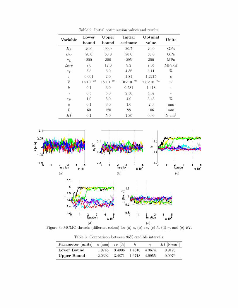
Table 2: Initial optimization values and results.

VariableLower Upper Initial Optimal

Unitsbound bound estimate value

EA 20.0 90.0 30.7 20.0 GPa

EM 20.0 50.0 26.0 50.0 GPa

σL 200 350 295 350 MPa

∆σT 7.0 12.0 9.2 7.04 MPa/K

εT 3.5 6.0 4.36 5.11 %

τ 0.001 2.0 1.81 1.2275 s

V 1×10−28 1×10−23 1.0×10−25 7.5×10−24 m3

h 0.1 3.0 0.581 1.418 -

γ 0.5 5.0 2.50 4.62 -

εP 1.0 5.0 4.0 3.43 %

a 0.1 3.0 1.0 2.0 mm

L 60 120 88 106 mm

EI 0.1 5.0 1.30 0.99 N-cm2

(a) (b) (c)

(d) (e)

Figure 3: MCMC threads (different colors) for (a) a, (b) εP , (c) h, (d) γ, and (e) EI.

Table 3: Comparison between 95% credible intervals.

Parameter [units] a [mm] εP [%] h γ EI [N-cm2]

Lower Bound 1.9746 3.4006 1.4310 4.3674 0.9123

Upper Bound 2.0392 3.4871 1.6713 4.9955 0.9976

(a) (b) (c)

(d) (e)

Figure 4: MCMC histograms for (a) a, (b) εP , (c) h, (d) γ, and (e) EI.

parallel thread follows a different path, they are all initialized at the same point. It may advantageous to usingdifferent initial values.

Future work will compare different proposal functions and their effect on the convergence of the posteriordensity. Additionally, MCMC results will be compared to other uncertainty quantification approaches such asbootstrapping. Ultimately, the results will be used in robust control algorithms.

Acknowledgments

This research was supported in part by the Air Force Office of Scientific Research through the grant AFOSRFA9550-11-10152.

REFERENCES

1. Veeramani, A., Buckner, G., Owen, S., Bolotin, G., and Cook, R., “Modeling the dynamic behavior of ashape memory alloy actuated catheter,” Smart Materials and Structures 19(1), 1–14 (2008).

2. Crews, J. and Buckner, G., “Design optimization of a shape memory alloy actuated robotic catheter,”Journal of Intelligent Material Systems and Structures (2011).

3. Laurentis, K. D. and Mavroidis, C., “Mechanical design of a shape memory alloy actuated prosthetic hand,”Technology and Health Care 10, 91–106 (2002).

4. Hartl, D., Lagoudas, D., Calkins, F., and Mabe, J., “Use of a ni60ti shape memory alloy for active jetengine chevron application: I. thermomechanical characterization,” Smart Materials and Structures 19,1–14 (2010).

5. Hartl, D., Lagoudas, D., Calkins, F., and Mabe, J., “Use of a ni60ti shape memory alloy for active jet enginechevron application: II. experimentally validated numerical analysis,” Smart Materials and Structures 19,1–14 (2010).

6. Garner, L., Wilson, L., Lagoudas, D., and Rediniotis, O., “Development of a shape memory alloy actuatedbiomimetic vechicle,” Smart Materials and Structures 9, 673–683 (2000).

7. Kaipio, J. and Somersalo, E., [Statistical and computational inverse problems ], vol. 160, Springer Verlag(2005).

8. Gelman, A., [Bayesian data analysis ], CRC press (2004).

9. Solonen, A., Monte Carlo methods in parameter estimation of nonlinear models, Master’s thesis, Lappeen-rante University of Technology (2006).

10. Khalil, H., [Nonlinear Systems ], Prentice Hall (2002).

11. Smith, R., [Smart Material Systems: Model Development ], SIAM, Philadelphia (2005).

12. Smith, R., Seelecke, S., Dapino, M., and Ounaies, Z., “A unified framework for modeling hysteresis in ferroicmaterials,” Journal of Mechanics and Physics of Solids 54, 46–85 (2005).

13. Smith, R., Dapino, M., Braun, T., and Mortensen, A., “A homogenized energy framework for ferromagnetichysteresis,” IEEE Transactions on Magnetics 42(7) (2006).

14. Smith, R., Seelecke, S., Ounaies, Z., and Smith, J., “A free energy model for hysteresis in ferroelectricmaterials,” Journal of Intelligent Material Systems and Structures 14(11), 719–739 (2003).

15. Smith, R., Hatch, A., Mukherjee, B., and Liu, S., “A homogenized energy model for hysteresis in ferroelectricmaterials: General density formulation,” Journal of Intelligent Material Systems and Structures 16, 713–732(2005).

16. Smith, R., Seelecke, S., Dapino, M., and Ounaies, Z., “A unified framework for modeling in hystersis inferroic materials,” Journal of the Mechanics and Physics of Solids 54, 46–85 (2005).

17. Crews, J., Smith, R., Pender, K., Hannen, J., and Buckner, G., “Data-driven estimation of the homogenizedenergy model parameters for shape memory alloys,” Journal of Intelligent Material Systems and Structures(2011). Submitted.

18. Hu, Z., Smith, R., and Ernstberger, J., “The homogenized energy model (HEM) for characterizing polariza-tion and strains in hysteretic ferroelectric materials: implementation algorithms and data-driver parameterestimation techniques,” Journal of Intelligent Material Systems and Structures (2011). Submitted.

19. Hu, Z., Smith, R., and Ernstberger, J., “Data driven techniques to estimate parameters in a rate-dependentferromagnetic hysteresis model,” Physica:B . To appear.

20. Hu, Z., Smith, R., Stuebner, M., Hay, M., and Oates, W., “Statistical parameter estimation for macro fibercomposite actuators using the homogenized energy model,” 797806, Proceedings of the SPIE 7978 (2011).

21. Furst, S., Hangekar, R., and Seelecke, S., “Practical implementation of resistance feedback measurementfor position control of a flexible smart inhaler nozzle,” in [ASME 2010 Conference on Smart Materials,Adaptive Structures, and Intelligent Systems ], (2010).

22. Furst, S. and Seelecke, S., “Experimental validation of different methods for controlling a flexible nozzleusing embedded sma wires as both positioning actuator and sensor,” 79781K, Proceedings of the SPIE7978 (2011).

23. Crews, J., Development of a shape memory alloy actuated robotic catheter for endocardial ablation: modeling,design optimization, and control, PhD thesis, North Carolina State University (2011).

24. Cao, R., “An overview of bootstrap methods for estimating and predicting in time series,” Sociedad deEstadistic e Investagacion Operative Test 8, 95–116 (1999).

25. Zoubir, A. and Iskander, D., “Boostrap methods and applications,” IEEE Signal Processing Magazine 24,10–19 (2007).

26. Liu, R., “Bootstrap procedures under some non-i.i.d. models,” The Annals of Statistics 16, 1696–1708(1988).

27. Chib, S. and Greenberg, E., “Understanding the metropolis-hastings algorithm,” American Statistician ,327–335 (1995).

28. Andrieu, C. and Thoms, J., “A tutorial on adaptive mcmc,” Statistics and Computing 18(4), 343–373(2008).

29. Hannen, J., Crews, J., and Buckner, G., “Indirect intelligent sliding mode control of a shape memory alloyactuated flexible beam using hysteretic recurrent neural networks,” Smart Materials and Structures (2011).Submitted.