Comparison of Bayesian Parameter Estimation and Least

Comparison of Bayesian Parameter Estimation andLeast Squares Minimization for Inverse Grey-Box

Building Model Identification

Submitted to:

Prof. R. Balaji

Prepared by:

Greg PavlakDecember 14, 2011

Abstract

Bayesian parameter estimation and nonlinear least squares minimization are used for InverseGrey-Box model identification of a retail and large commercial office model. Detailed simulationengine EnergyPlus is used to generate surrogate data for estimation of parameters, and optimalparameters are compared through annual simulation of building zone temperature and thermalloads. A brief overview of Bayesian estimation techniques is provided, along with ideas forimprovements and future work.

Acknowledgements

I would like to acknowledge my colleague Anthony Florita for generously providing a MAT-LAB Bayesian parameter estimation routine and kindly offering his knowledge of Bayesianstatistics.

Contents

1 Introduction 1

2 Detailed Building Models 1

3 Reduced Order Model Structure 2

4 Least Squares Parameter Estimation 4

5 Bayesian Parameter Estimation 5

6 Results 6Retail Model Parameter Estimation . . . . . . . . . . . . . . . . . . . . . . . . . . . . . . 6Large Office Model Parameter Estimation . . . . . . . . . . . . . . . . . . . . . . . . . . . 10

7 Conclusion 13

8 Future Work 14

List of Figures

1 5 Zone Retail Building Model . . . . . . . . . . . . . . . . . . . . . . . . . . . . . . . 12 15 Zone Office Building Model . . . . . . . . . . . . . . . . . . . . . . . . . . . . . . 13 5 Paramater Thermal RC Network . . . . . . . . . . . . . . . . . . . . . . . . . . . . 24 Retail: R1R2 Posterior Contour . . . . . . . . . . . . . . . . . . . . . . . . . . . . . . 65 Retail: R1R3 Posterior Contour . . . . . . . . . . . . . . . . . . . . . . . . . . . . . . 66 Retail: R1Rw Posterior Contour . . . . . . . . . . . . . . . . . . . . . . . . . . . . . 77 Retail: R1C Posterior Contour . . . . . . . . . . . . . . . . . . . . . . . . . . . . . . 78 Retail: R2R3 Posterior Contour . . . . . . . . . . . . . . . . . . . . . . . . . . . . . . 79 Retail: R2Rw Posterior Contour . . . . . . . . . . . . . . . . . . . . . . . . . . . . . 710 Retail: R2C Posterior Contour . . . . . . . . . . . . . . . . . . . . . . . . . . . . . . 811 Retail: R3Rw Posterior Contour . . . . . . . . . . . . . . . . . . . . . . . . . . . . . 812 Retail: R3C Posterior Contour . . . . . . . . . . . . . . . . . . . . . . . . . . . . . . 813 Retail: RwC Posterior Contour . . . . . . . . . . . . . . . . . . . . . . . . . . . . . . 814 Retail: Cooling Load Comparision . . . . . . . . . . . . . . . . . . . . . . . . . . . . 915 Retail: Zone Mean Air Temperature Comparison . . . . . . . . . . . . . . . . . . . . 916 Office: R1R2 Posterior Contour . . . . . . . . . . . . . . . . . . . . . . . . . . . . . . 1017 Office: R1R3 Posterior Contour . . . . . . . . . . . . . . . . . . . . . . . . . . . . . . 1018 Office: R1Rw Posterior Contour . . . . . . . . . . . . . . . . . . . . . . . . . . . . . 1019 Office: R1C Posterior Contour . . . . . . . . . . . . . . . . . . . . . . . . . . . . . . 1020 Office: R2R3 Posterior Contour . . . . . . . . . . . . . . . . . . . . . . . . . . . . . . 1121 Office: R2Rw Posterior Contour . . . . . . . . . . . . . . . . . . . . . . . . . . . . . 1122 Office: R2C Posterior Contour . . . . . . . . . . . . . . . . . . . . . . . . . . . . . . 1123 Officel: R3Rw Posterior Contour . . . . . . . . . . . . . . . . . . . . . . . . . . . . . 1124 Office: R3C Posterior Contour . . . . . . . . . . . . . . . . . . . . . . . . . . . . . . 11

25 Office: RwC Posterior Contour . . . . . . . . . . . . . . . . . . . . . . . . . . . . . . 1126 Office: Cooling Load Comparision . . . . . . . . . . . . . . . . . . . . . . . . . . . . 1227 Office: Zone Mean Air Temperature Comparison . . . . . . . . . . . . . . . . . . . . 13

List of Tables

1 Selected EnergyPlus Model Details . . . . . . . . . . . . . . . . . . . . . . . . . . . . 22 Reduced Order Model Parameter Bounds . . . . . . . . . . . . . . . . . . . . . . . . 53 Retail Model Parameter Estimates . . . . . . . . . . . . . . . . . . . . . . . . . . . . 84 Office Model Parameter Estimates . . . . . . . . . . . . . . . . . . . . . . . . . . . . 12

1 Introduction

Advanced building control and fault detection methods utilize building energy models to pre-dict or estimate expected building performance. Online implementation of such methods requireslight-weight, computationally efficient models that capture the critical system dynamics. InverseGrey-Box models have shown the potential for blending the benefits of building physics knowledgewith measured performance data. Inverse Grey-Box building models have been successfully usedto predict cooling loads and energy consumption for optimal control strategy evaluation, as well asonline next-day load predictions [1],[2], [8]. Extended Kalman Filters (EKF) have also been incor-porated with similar model structures to improve real-time load estimates using available BAS data[5]. Various model identification techniques have been demonstrated that typically involve time orfrequency domain least squares minimization via traditional (e.g. Gauss-Newton) or metaheuristic(e.g. genetic) algorithms . Lauret et al. demonstrated the use of Bayesian parameter estimation indetermining better estimates of the inputs for roof-mounted radiant barrier system forward model[4]. This paper applies Bayesian parameter estimation methods to Inverse Grey-Box models andprovides comparison with least squares model identification.

2 Detailed Building Models

Detailed simulation engine EnergyPlus was used generate surrogate surrogate data for two buildingmodels: 1) a 5 zone retail building and 2) a 15 zone office building. The load calculations from thesedetailed simulations is used as ”measured” training data for the reduced order models. Figures 1and 2 illustrate model geometry, and Table 1 highlights selected model details.

Figure 1: 5 Zone Retail Building Model Figure 2: 15 Zone Office Building Model

1

Table 1: Selected EnergyPlus Model Details

Property Retail Office Units

Floors 1 32 floorsTotal Floor Area 2300 77000 m2

Occupancy 7.11 51.8 m2/personLighting 32.3 9.8 W/m2

Appliance 5.23 4.63 W/m2

3 Reduced Order Model Structure

Inverse Grey-Box models are based on the approximation of heat transfer mechanisms with ananalogous electrical lumped resistance-capacitance network. This approximation creates a flexiblestructure that allows the modeler to choose an appropriate level of abstraction. Model complexitycan range from representing entire systems with a few parameters, to modeling each heat transfersurface with numerous parameters. Depending on the model structure and complexity, modelparameters can approximate physical characteristics of the system. Model parameters are thenidentified thought a training period with measured data. For this work, a 5 parameter model, shownin Figure 3, based on ISO13790 was used to predict summer cooling loads for a small retail and largeoffice building [3]. Heat transfer through the opaque building shell materials is represented by R1,

R1 R2 R3

Rw

C

Ta

Ta

Tm TsTz

Qg,r+sol,w Qgc

Figure 3: 5 Paramater Thermal RC Network

R2, and C. These elements link the ambient temperature node to an pseudo surface temperaturenode (Ts), accounting for potential heat storage of the mass materials. Glazing heat transfer isrepresented by a single resistance Rw connecting the ambient temperature node to the surfacetemperature node, as thermal storage of glazing is typically neglected. R3 represents a lumpedconvection/radiation coefficient between the surface temperature node and zone air temperaturenode Tz. The convective portion of internal gains (lighting, occupants, and equipment) are appliedas a direct heat source to the zone temperature node, shown as Qgc, and the radiant fractionalong with glazing transmitted solar gains (Qg,r+sol,w) are applied to the surface node. Although,convective and radiative splits are made, radiative heat transfer mechanisms are lumped together

2

in R3.An energy balance can be written on the mass temperature node Tm, as

CdTmdt

=Ta − TmR1

+Ts − TmR2

(1)

Since no storage occurs at the surface node, flows entering and leaving the node sum to zero.

Ta − TsRw

+Tz − TsR3

+Tm − TsR2

+ Qg,r+sol,w = 0 (2)

The heat gain to the space is then represented by the total heat flow to the zone air node.

Qsh =Ts − TzR3

+ Qgc (3)

Equations 1 - 4 form a first order differential equation that can be rewritten in state space form

x = Ax + Bu

y = cx + du

with non-zero matrix elements

A(1, 1) =1

C

(−1

R1+−1

R2+

RwR3

R2R3 +RwR2 +RwR3

)

B(1, 1) =1

C

(Rw

R2R3 +RwR2 +RwR3

)

B(1, 2) =1

C

(R3

R2R3 +RwR2 +RwR3

)

B(1, 3) =1

R1C

B(1, 6) =1

C

(RwR3

R2R3 +RwR2 +RwR3

)

B(1, 7) =1

C

(R2R3

R2R3 +RwR2 +RwR3

)

B(1, 8) =1

C

(R2R3

R2R3 +RwR2 +RwR3

)

C(1) =Rw

R2R3 +RwR2 +RwR3

D(1) =−1

R3+

RwR2

R3 (R2R3 +RwR2 +RwR3)

D(2) =R2

R2R3 +RwR2 +RwR3

D(6) =RwR2

R2R3 +RwR2 +RwR3)

D(7) =RwR2

R2R3 +RwR2 +RwR3)

D(8) =RwR2

R2R3 +RwR2 +RwR3)

D(9) = 1

and state and input vectors described as

xT = [Tm]

uT = [Tz Ta Tg Qsol,c Qsol,e Qg,r,c Qg,r,e Qsol,w Qg,c]

3

Tz is the zone temperature setpoint, Ta is the ambient external temperature, Qsol,c is the externalsolar gains incident on the roof, Qsol,e is the solar radiation incident on exterior walls, Qg,r,c is theradiative portion of internal gains applied to the ceiling surface node, Qg,r,e is the radiative portionof internal gains applied to the wall surface node, Qsol,w is the solar radiation transmitted throughglazing, and Qg,c is the total convective internal gains.

The state space equations are then converted to the following heat transfer function presented byBraun [1], and the conversion process is described by Seem [6].

Qsh,t =n∑k=0

STk ut−k∆τ −m∑k=1

ekQsh,t−k∆τ (4)

The transfer function method is an efficient calculation method as it relates the sensible heat gainsto the space (Qsh) at time t to the inputs of n and heat gains of m previous timesteps. Equation4 is used to perform load calculations for the zone that include the effects of dual temperaturesetpoints with deadbands and system capacity limitations.

Zone temperature predictions are also made using an inverse form of Equation 4.

Tz =

9∑l=2

S0(l)ut(l) +8∑j=1

Sjut−j∆τ −8∑j=1

ekQsh,t−j∆τ + 2 Cz∆τ Tz,t−∆τ + minfCput(2) + Qzs,t

2 Cz∆τ − S0(1) + minfCp

(5)

Tz,t = 2Tz,t − Tz,t−∆τ

4 Least Squares Parameter Estimation

As a first approach to model identification, least squares minimization was used to identify modelparameters that minimize the root-mean-squared error (RMSE), defined by Equation 6, between thereduced order model and EnergyPlus load calculations. A two stage optimization was implementedthat first performs a direct search over the parameter space to identify a starting point for localrefinement. The direct search is performed on p uniform random points located within the bounds ofthe parameter space. The local refinement, subject to the same parameter constraints, is performedvia nonlinear least squares minimization implemented using a built-in MATLAB optimizer basedon trust-region methods [7].

J =

√√√√√ N∑i=1

(Qd,i − Qzs,i)2

N(6)

For this study, 500 direct search points were used within the bounds listed in Table 2. The parameterestimation was repeated 1000 times, beginning each iteration with a new set of randomly generateddirect search points.

4

Table 2: Reduced Order Model Parameter Bounds

R1 R2 R3 Rw C1

Min 0 0 0.03030303 0.05 78.008832Max 4.988662132 4.988662132 33.33366667 3 536659.2

Units m2-K/W m2-K/W m2-K/W m2-K/W J/m2-K

5 Bayesian Parameter Estimation

Bayesian methods benefit over traditional methods in that an entire distribution of parameterprobabilities is developed and prior knowledge of the system can be incorporated in to the estimationtask. Specifically, the individual probabilities of events A and B

p(A), p(B)

are related to their conditional probabilities

p(A|B), p(B|A)

by Bayes’ Theorem (Eq. 7).

p(A|B) =p(B|A)p(A)

p(B)(7)

From a parameter estimation perspective, the probability of parameters Θ given measured data Dand a knowledge base of the system K can be written as posterior probability p(Θ|DK). Bayes’Theorem then allows the conditional probability p(Θ|DK) to be computed from p(Θ|K), p(D|ΘK),and p(D|K) as in Equation 8,

p(Θ|DK) = p(Θ|K)p(D|ΘK)

p(D|K)(8)

where p(Θ|K) represents prior knowledge about parameter values, p(D|ΘK) represents the likeli-hood of observing the measured dataset D given a particular parameter set and knowledge of thesystem, and p(D|K) is the probability of randomly observing the dataset. The relation can bewritten in alternate form where the numerator remains the product of likelihood and prior, anddenominator is a normalization factor so that posterior probabilities sum to unity.

p(Θ|D) =p(Θ)p(D|Θ)∑

ip(Θi)p(D|Θi)

(9)

Assuming random Gaussian noise about the measured data, the probability of an observation canbe determined from its location under the normal distribution centered at µ equal to the measuredvalue, with standard deviation σε.

p(Oi|Θ) =1

σε√

2πexp(

−(Oi −Mi)2

2σ2ε

) (10)

5

Assuming independent errors, the likelihood of the entire dataset is simply the product of likelihoodsof all individual points.

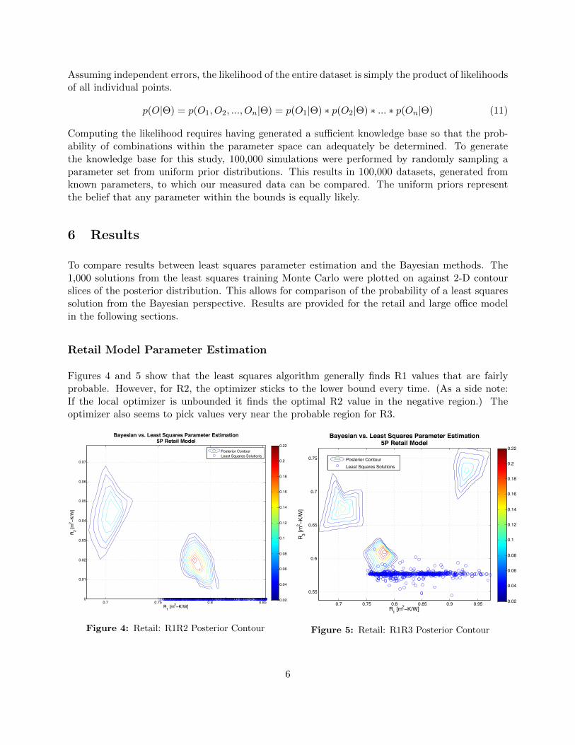
p(O|Θ) = p(O1, O2, ..., On|Θ) = p(O1|Θ) ∗ p(O2|Θ) ∗ ... ∗ p(On|Θ) (11)

Computing the likelihood requires having generated a sufficient knowledge base so that the prob-ability of combinations within the parameter space can adequately be determined. To generatethe knowledge base for this study, 100,000 simulations were performed by randomly sampling aparameter set from uniform prior distributions. This results in 100,000 datasets, generated fromknown parameters, to which our measured data can be compared. The uniform priors representthe belief that any parameter within the bounds is equally likely.

6 Results

To compare results between least squares parameter estimation and the Bayesian methods. The1,000 solutions from the least squares training Monte Carlo were plotted on against 2-D contourslices of the posterior distribution. This allows for comparison of the probability of a least squaressolution from the Bayesian perspective. Results are provided for the retail and large office modelin the following sections.

Retail Model Parameter Estimation

Figures 4 and 5 show that the least squares algorithm generally finds R1 values that are fairlyprobable. However, for R2, the optimizer sticks to the lower bound every time. (As a side note:If the local optimizer is unbounded it finds the optimal R2 value in the negative region.) Theoptimizer also seems to pick values very near the probable region for R3.

R1 [m2−K/W]

R 2 [m2 −

K/W

]

Bayesian vs. Least Squares Parameter Estimation5P Retail Model

0.7 0.75 0.8 0.850

0.01

0.02

0.03

0.04

0.05

0.06

0.07

Posterior ContourLeast Squares Solutions

0.02

0.04

0.06

0.08

0.1

0.12

0.14

0.16

0.18

0.2

0.22

Figure 4: Retail: R1R2 Posterior Contour

R1 [m2−K/W]

R 3 [m2 −

K/W

]


0.7 0.75 0.8 0.85 0.9 0.95

0.55

0.6

0.65

0.7

0.75 Posterior ContourLeast Squares Solutions

0.02

0.04

0.06

0.08

0.1

0.12

0.14

0.16

0.18

0.2

0.22


6

Figures 6 and 7 show that several solutions are found within the probable region of Rw, howeverthere does not appear to be great consistency. Capacitance values appear cluster between regionsof lower probability.

R1 [m2−K/W]

R w [m2 −

K/W

]


0.4 0.5 0.6 0.7 0.8 0.9

0.8

0.9

1

1.1

1.2

1.3


0.02

0.04

0.06

0.08

0.1

0.12

0.14

0.16

Figure 6: Retail: R1Rw Posterior Contour

R1 [m2−K/W]C

J/[m

2 −K]

Bayesian vs. Least Squares Parameter EstimationRetail Model

0.5 1 1.5 2 2.5 3 3.5 4 4.53.5

4

4.5

5

5.5 x 105


0.05

0.1

0.15

0.2

0.25

Figure 7: Retail: R1C Posterior Contour

Figure 8 again shows the lower boundary local optimizer choice for R2, and that R3 values arewithin the probable range. Figure 9 again shows the range of window resistances in and outside ofprobable ranges.

R2 [m2−K/W]

R 3 [m2 −

K/W

]


0 0.01 0.02 0.03 0.04 0.05 0.06 0.07

0.5

0.55

0.6

0.65

0.7

0.75


0.05

0.1

0.15

0.2


R2 [m2−K/W]

R w [m2 −

K/W

]


0 0.01 0.02 0.03 0.04 0.05 0.06 0.07 0.08 0.09 0.1

0.1

0.2

0.3

0.4

0.5

0.6

0.7

0.8

0.9

1

1.1Posterior ContourLeast Squares Solutions

0.01

0.015

0.02

0.025

0.03

0.035

0.04

0.045

0.05

0.055

0.06


Figure 10 - 13 highlights the above results in a different manner by plotting the remaining com-binations of posterior slices. Table 3 compares the median estimate from the 1000 nonlinear leastsquares trainings to the most probable Bayesian estimate.

7

R2 [m2−K/W]

C [J

/m2 −

K]Bayesian vs. Least Squares Parameter Estimation

Retail Model

0 0.02 0.04 0.06 0.08 0.1 0.12 0.14 0.16 0.18

3.6

3.8

4

4.2

4.4

4.6

4.8

5

5.2

5.4x 105


0.05

0.1

0.15

0.2


R3 [m2−K/W]

R w [m2 −

K/W

]


0.48 0.5 0.52 0.54 0.56 0.58 0.6 0.62 0.64 0.66

0.2

0.4

0.6

0.8

1


0.02

0.04

0.06

0.08

0.1

0.12

0.14

0.16

0.18

0.2


R3 [m2−K/W]

C [J

/m2 −

K]


0 0.5 1 1.5 2 2.5 3

3.2

3.4

3.6

3.8

4

4.2

4.4

4.6

4.8

5

5.2

x 105


0.05

0.1

0.15

0.2


Rw [m2−K/W]

C [J

/m2 −

K]Bayesian vs. Least Squares Parameter Estimation

Retail Model

0.5 1 1.5 2 2.5

0.5

1

1.5

2

2.5

3

3.5

4

4.5

5

x 105


0.01

0.02

0.03

0.04

0.05

0.06

0.07

0.08

0.09

0.1

Figure 13: Retail: RwC Posterior Contour

Table 3: Retail Model Parameter Estimates

R1 R2 R3 Rw C

Upper Bound 4.989 4.989 33.334 3.000 536659NLSQ 0.849 0.000 0.577 0.184 504866Bayes 0.784 0.018 0.613 0.795 352421Lower Bound 0.000 0.000 0.030 0.050 78


The best parameter set from each method were used to perform an annual simulation of the buildingheating and cooling loads. The predicted thermal loads and zone temperatures are shown in Figures

8

14 and 15, respectively. Overall, the performance is virtually the same for the period shown. Theannual RMSE of the load profiles increased by 4% with the Bayesian solution.

3840 3860 3880 3900 3920 3940 3960 3980 4000 4020 4040

−10

−9

−8

−7

−6

−5

−4

−3

−2

−1

0x 104

Time [hours]

Zone

Sen

sibl

e Lo

ad[W

]

Nonlinear Least Squares vs. Bayesian Parameter Estimation: Cooling Loads

EnergyPlus05P (least squares)05P (Bayesian)

Figure 14: Retail: Cooling Load Comparision

3840 3860 3880 3900 3920 3940 3960 3980 4000 4020 404015

20

25

30

Time [hours]

Zone

Mea

n Ai

r Tem

pera

ture

[C]

Nonlinear Least Squares vs. Bayesian Parameter Estimation: Zone Temperatures

EnergyPlus05P (least squares)05P (Bayesian)Heating SPCooling SP

Figure 15: Retail: Zone Mean Air Temperature Comparison

9

Large Office Model Parameter Estimation

The same analysis was repeated, training the 5 parameter model to data from a large 32 story officebuilding. It should be noted that some level of mismatch inherently exists between the simple 5parameter model and complex office building. It seems that the 5 parameter model may be overlysimple for this type of building, regardless of parameter estimation technique. Values for R2 andR3 are chosen near Bayesian probable locations, however the remaining parameter selection end upquite different. Figures 16 - 25 plot combinations of parameter slices for visualizing the estimationresults.

R1 [m2−K/W]

R 2 [m2 −

K/W

]

Bayesian vs. Least Squares Parameter EstimationLarge Office Model

0.73 0.74 0.75 0.76 0.77 0.78 0.79 0.8 0.81 0.820.11

0.115

0.12

0.125

0.13

0.135


0.05

0.1

0.15

0.2

0.25

0.3

0.35

0.4

0.45

0.5

0.55

Figure 16: Office: R1R2 Posterior Contour

R1 [m2−K/W]

R 3 [m2 −

K/W

]


0.8 1 1.2 1.4 1.6 1.80

0.02

0.04

0.06

0.08

0.1

0.12


0.02

0.04

0.06

0.08

0.1

0.12

0.14


R1 [m2−K/W]

R w [m2 −

K/W

]


0.8 1 1.2 1.4 1.6 1.8 20.6

0.7

0.8

0.9

1

1.1

1.2

1.3

1.4

1.5


0.05

0.1

0.15

0.2

0.25

0.3

0.35

0.4

0.45

0.5

0.55

Figure 18: Office: R1Rw Posterior Contour

R1 [m2−K/W]

C [J

/m2 −

K]

Bayesian vs. Least Squares Parameter EstimationLarge Office

0.5 1 1.5 2 2.5 3 3.5 4 4.5

4.5

4.6

4.7

4.8

4.9

5

5.1

5.2

x 105


0.1

0.15

0.2

0.25

0.3

0.35

0.4

0.45

0.5

0.55

0.6

Figure 19: Office: R1C Posterior Contour

10

R2 [m2−K/W]

R 3 [m2 −

K/W

]


0.08 0.09 0.1 0.11 0.12 0.130.02

0.03

0.04

0.05

0.06

0.07

0.08


0.1

0.15

0.2

0.25

0.3

0.35

0.4

0.45

0.5

0.55

0.6


R2 [m2−K/W]

R w [m2 −

K/W

]


0.08 0.09 0.1 0.11 0.12 0.130.5

0.6

0.7

0.8

0.9

1

1.1

1.2

1.3

1.4


0.1

0.15

0.2

0.25

0.3

0.35

0.4

0.45

0.5

0.55

0.6

Figure 21: Office: R2Rw Posterior Contour

R2 [m2−K/W]

C [J

/m2 −

K]

Bayesian vs. Least Squares Parameter EstimationLarge Office

0.05 0.1 0.15 0.2 0.25 0.3 0.35 0.4 0.45 0.5

2.5

3

3.5

4

4.5

5

x 105


0.01

0.02

0.03

0.04

0.05

0.06

0.07

0.08

0.09

0.1

0.11


R3 [m2−K/W]

R w [m2 −

K/W

]


0.03 0.04 0.05 0.06 0.07 0.08

0.6

0.8

1

1.2

1.4

1.6


0.1

0.15

0.2

0.25

0.3

0.35

0.4

0.45

0.5

0.55

0.6

Figure 23: Officel: R3Rw Posterior Contour

R3 [m2−K/W]

C [J

/m2 −

K]


0 0.5 1 1.5 2

4.4

4.5

4.6

4.7

4.8

4.9

5

5.1

5.2

x 105


0.1

0.15

0.2

0.25

0.3

0.35

0.4

0.45

0.5

0.55

0.6


Rw [m2−K/W]

C [J

/m2 −

K]


0.6 0.8 1 1.2 1.4 1.6 1.8 2 2.2

4.4

4.5

4.6

4.7

4.8

4.9

5

5.1

5.2

5.3x 105


0.05

0.1

0.15

0.2

0.25

0.3

0.35

0.4

Figure 25: Office: RwC Posterior Contour

11

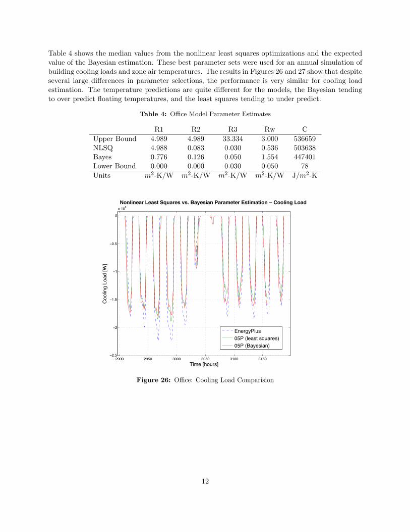
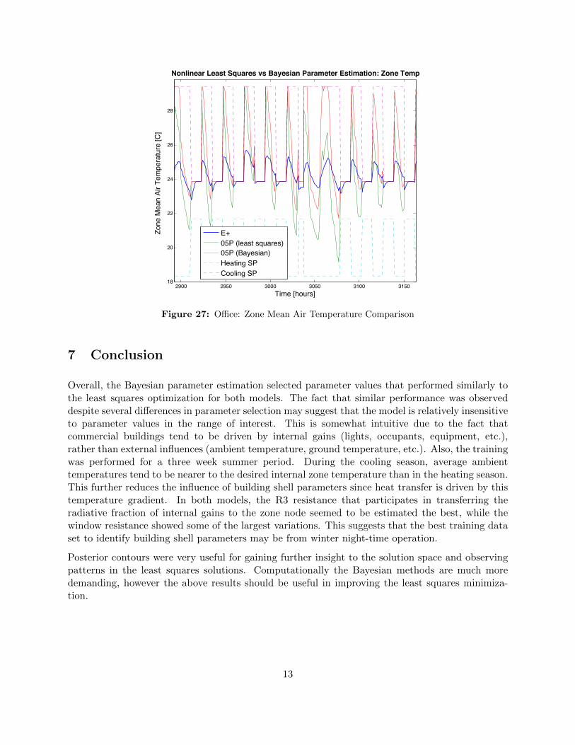
Table 4 shows the median values from the nonlinear least squares optimizations and the expectedvalue of the Bayesian estimation. These best parameter sets were used for an annual simulation ofbuilding cooling loads and zone air temperatures. The results in Figures 26 and 27 show that despiteseveral large differences in parameter selections, the performance is very similar for cooling loadestimation. The temperature predictions are quite different for the models, the Bayesian tendingto over predict floating temperatures, and the least squares tending to under predict.

Table 4: Office Model Parameter Estimates

R1 R2 R3 Rw C

Upper Bound 4.989 4.989 33.334 3.000 536659NLSQ 4.988 0.083 0.030 0.536 503638Bayes 0.776 0.126 0.050 1.554 447401Lower Bound 0.000 0.000 0.030 0.050 78


2900 2950 3000 3050 3100 3150−2.5

−2

−1.5

−1

−0.5

0

x 106Nonlinear Least Squares vs. Bayesian Parameter Estimation − Cooling Load

Time [hours]

Coo

ling

Load

[W]

EnergyPlus05P (least squares)05P (Bayesian)

Figure 26: Office: Cooling Load Comparision

12

2900 2950 3000 3050 3100 315018

20

22

24

26

28

Time [hours]

Zone

Mea

n Ai

r Tem

pera

ture

[C]

Nonlinear Least Squares vs Bayesian Parameter Estimation: Zone Temp

E+05P (least squares)05P (Bayesian)Heating SPCooling SP

Figure 27: Office: Zone Mean Air Temperature Comparison

7 Conclusion

Overall, the Bayesian parameter estimation selected parameter values that performed similarly tothe least squares optimization for both models. The fact that similar performance was observeddespite several differences in parameter selection may suggest that the model is relatively insensitiveto parameter values in the range of interest. This is somewhat intuitive due to the fact thatcommercial buildings tend to be driven by internal gains (lights, occupants, equipment, etc.),rather than external influences (ambient temperature, ground temperature, etc.). Also, the trainingwas performed for a three week summer period. During the cooling season, average ambienttemperatures tend to be nearer to the desired internal zone temperature than in the heating season.This further reduces the influence of building shell parameters since heat transfer is driven by thistemperature gradient. In both models, the R3 resistance that participates in transferring theradiative fraction of internal gains to the zone node seemed to be estimated the best, while thewindow resistance showed some of the largest variations. This suggests that the best training dataset to identify building shell parameters may be from winter night-time operation.

Posterior contours were very useful for gaining further insight to the solution space and observingpatterns in the least squares solutions. Computationally the Bayesian methods are much moredemanding, however the above results should be useful in improving the least squares minimiza-tion.

13

8 Future Work

Similar analysis could be repeated for models of higher complexity. Currently six Inverse Grey-Boxmodels exist ranging from 5 to 21 parameters. As model complexity increase, several parameters canmodel similar characteristics. It would be interesting to see if parameter tradeoffs are observed in theposterior distributions by areas of equally high probability. The estimation could also be extendedto incorporate hierarchical models to investigate parameter covariance quantitatively.

The results are also sensitive to the measurement error σε. Lauret et al. provide some insight intodealing with this by incorporating it as a free parameter in the estimation [4]. This technique couldbe implemented as the current environment requires trial and error to find an appropriate value.(If σε is too large, then everything is similarly likely and the posterior is useless. If σε is to small,nothing is likely and the posterior is zero everywhere.)

Improvements in the least squares training method are also planned. The total least squares couldbe minimized between the temperature and load profiles, and the effects of various training perioddurations and seasons could be explored as well. State correction as a function of past deviationsmay also be explored.

14

References

[1] J. E. Braun, Ph.D. and N. Chaturvedi, An Inverse Gray-Box Model for Transient BuildingLoad Prediction, HVAC&R Research, 8 (2002), pp. 73–100.

[2] J. E. Braun, Ph.D., K. W. Montgomery, and N. Chaturvedi, Evaluating the Perfor-mance of Building Thermal Mass Control Strategies, HVAC&R Research, 7 (2001), pp. 403–428.

[3] ISO, INTERNATIONAL STANDARD ISO 13790, tech. rep., International Organization forStandardization, 2008.

[4] P. Lauret, Bayesian parameter estimation of convective heat transfer coefficients of a roof-mounted radiant barrier system, Journal of Solar Energy Engineering, 128 (2006), pp. 213 –225.

[5] Z. O’Neill, S. Narayanan, and R. Brahme, MODEL-BASED THERMAL LOAD ESTI-MATION IN BUILDINGS, in Fourth National Conference of IBPSA-USA, New York, 2010.

[6] J. Seem, Modeling of Heat Transfer in Buildings, PhD thesis, University of Wisconsin-Madison,1987.

[7] I. The MathWorks, lsqnonlin, tech. rep., MATLAB help files, 2011.

[8] Q. Zhou, S. Wang, X. Xu, and F. Xiao, A grey-box model of next-day building thermalload prediction for energy-efficient control, International Journal of Energy Research, (2008),pp. 1418–1431.

15

Documents

Comparison of Bayesian Parameter Estimation and Least