IT 16 052

Examensarbete 30 hpJuni 2016

Bayesian parameter estimation in Ecolego using an adaptive Metropolis-Hastings-within-Gibbs algorithm

Sverrir Þorgeirsson

Institutionen för informationsteknologiDepartment of Information Technology

Teknisk- naturvetenskaplig fakultet UTH-enheten Besöksadress: Ångströmlaboratoriet Lägerhyddsvägen 1 Hus 4, Plan 0 Postadress: Box 536 751 21 Uppsala Telefon: 018 – 471 30 03 Telefax: 018 – 471 30 00 Hemsida: http://www.teknat.uu.se/student

Abstract

Bayesian parameter estimation in Ecolego using anadaptive Metropolis-Hastings-within-Gibbs algorithm

Sverrir Þorgeirsson

Ecolego is scientific software that can be used to model diverse systems within fieldssuch as radioecology and pharmacokinetics. The purpose of this research is todevelop an algorithm for estimating the probability density functions of unknownparameters of Ecolego models. In order to do so, a general-purpose adaptiveMetropolis-Hastings-within-Gibbs algorithm is developed and tested on someexamples of Ecolego models. The algorithm works adequately on those models, whichindicates that the algorithm could be integrated successfully into future versions ofEcolego.

Tryckt av: Reprocentralen ITCIT 16 052Examinator: Edith NgaiÄmnesgranskare: Michael AshcroftHandledare: Rodolfo Avila

Contents1 Introduction 1

1.1 Previous work . . . . . . . . . . . . . . . . . . . . . . . . . . . . . 1

2 Problem definition and background 3

2.1 Compartment models . . . . . . . . . . . . . . . . . . . . . . . . 32.2 Ecolego . . . . . . . . . . . . . . . . . . . . . . . . . . . . . . . . 42.3 Statistical approaches . . . . . . . . . . . . . . . . . . . . . . . . 5

3 Markov Chain Monte Carlo methods 7

3.1 Markov chains . . . . . . . . . . . . . . . . . . . . . . . . . . . . 83.2 Markov Chain Monte Carlo Methods . . . . . . . . . . . . . . . . 8

3.2.1 Gibbs sampling . . . . . . . . . . . . . . . . . . . . . . . . 93.2.2 Metropolis-Hastings algorithm . . . . . . . . . . . . . . . 103.2.3 Metropolis-within-Gibbs . . . . . . . . . . . . . . . . . . . 133.2.4 Adaptive Metropolis-within-Gibbs . . . . . . . . . . . . . 14

3.3 Choice of initial values . . . . . . . . . . . . . . . . . . . . . . . . 153.4 Convergence checking . . . . . . . . . . . . . . . . . . . . . . . . 15

3.4.1 Gelman and Rubin . . . . . . . . . . . . . . . . . . . . . . 163.4.2 Raftery and Lewis . . . . . . . . . . . . . . . . . . . . . . 16

4 Implementation 18

5 Experiments and results 21

5.1 Exponential model with two variables . . . . . . . . . . . . . . . 215.2 Simple linear model with three parameters . . . . . . . . . . . . . 24

6 Conclusions 29

7 Future work 30

8 Bibliography 31

1 IntroductionEcolego is specialized software used by scientists to make inferences on the prop-erties and behavior of systems and their components in nature and elsewhere.The Ecolego user is expected to create a model as an abstraction of some real-life phenomena, specify parameters and measurements, run the model, and getsome meaningful output. However, for some applications it is desirable to turnthis process on its head; if a model M gives some output y, then what werethe parameters θ? This is called the inverse problem, a problem that is some-times considered “severely under-determined and ill-posed” when the amountof underlying data is small [Calvetti et al., 2006].

This thesis is about developing a general-purpose algorithm to solve theinverse problem of parameter estimation in Ecolego. The goal is not only toestimate the most likely values of the parameters but also to get probabilitydistributions of the variables in question. In order to do so, Bayesian statisticalmethods will be used.

Section 2 of this document contains some necessary background behind thework, including information on Ecolego and the fundamental statistical ideasused in order to write the software to solve the problem. It also explains whyBayesian statistical methods were preferred over other other possibilities. Sec-tion 3 also contains some background theory: a description of the algorithmused (see Sections 3.2.3 and 3.2.4) and related techniques within computationalstatistics.

Section 4 gives an overview of the technical implementation of the soft-ware and how the user is expected to interact with it. Section 5 documentsexperiments performed using the algorithm and Sections 6 and 7 contain theconclusion of the thesis and some discussion respectively.

The thesis is sponsored by the Stockholm company Facilia AB, the owner,creator and and developer of Ecolego.

1.1 Previous workA lot has been written on Bayesian statistical methods for inverse parameterestimation. Relevant sources on that topic have been listed in the section atthe end of this report and referenced throughout the text. Inverse parameterestimation in Ecolego is a more narrow topic, but in 2006, Martin Malhotrawrote a Master’s thesis on a related subject that was also sponsored by Fa-

1

cilia AB [Malhotra, 2006]. Malhotra’s thesis provided some of the theoreticalbackground behind the algorithm developed in this thesis.

In addition to Martin’s thesis, Kristofer Stenberg also wrote a Master’s the-sis sponsored by Facilia on Markov Chain Monte Carlo methods among otherrelated topics within finance [Stenberg, 2007]. Some ideas in Stenberg’s thesiswere discussed in this report where applicable.

2

2 Problem definition and background

2.1 Compartment modelsA compartment model, or a compartmental system, is a system consisting sub-units called compartments with each of them containing a homogeneous andwell-mixed material [Jacquez, 1996]. The state of the system is modified whenthe material flows from one compartment to another, or when the material en-ters or exits the system from an external source. According to Jacquez [1999], acompartment is simply an amount of this material with the requirement that thematerial is kinetically homogeneous, which means that it fulfills two conditions:

1. When added to a compartment, the material must be instantaneously anduniformly mixed with the existing material of the component.

2. When exiting a compartment, any small amount of the material must havethe same probability of exiting as any other small amount.

Furthermore, the model must contain equations that specify how the mate-rial flows from one compartment to another. Borrowing Jacquez’s notation, ifFij denotes the flow from compartment j to another compartment i per unitof time and qj is the amount of material in compartment j, then Fij = fij · qj

where fij is the transfer coefficient for compartments i and j. If the trans-fer coefficient for every pair of distinct compartments is a constant, then thecompartmental system is considered to be linear, if at least one transfer coeffi-cient is depending on time and the rest are constants, then the system is linear

with time-varying coefficients, and finally if at least one transfer coefficient isa function of some qx then the system is nonlinear [Jacquez, 1999]. In otherwords, within a linear compartment model, the rate of transfer from any com-partment j to another compartment i is proportional to the current amount ofmaterial in compartment j. In nonlinear compartment models, there is no suchrequirement.

Compartment models, linear or not, can be used to model a variety of sys-tems and experiments in nature. According to Seber and Wild (2003), theyare also an important tool in biology, physiology, pharmacokinetics, chemistryand biochemistry. Compartmental systems have been used for purposes such asmodeling the movement of lead in the human body, how bees pick up radioac-tivity and a food chain in the Aleutian Islands [Seber and Wild, 2003].

3

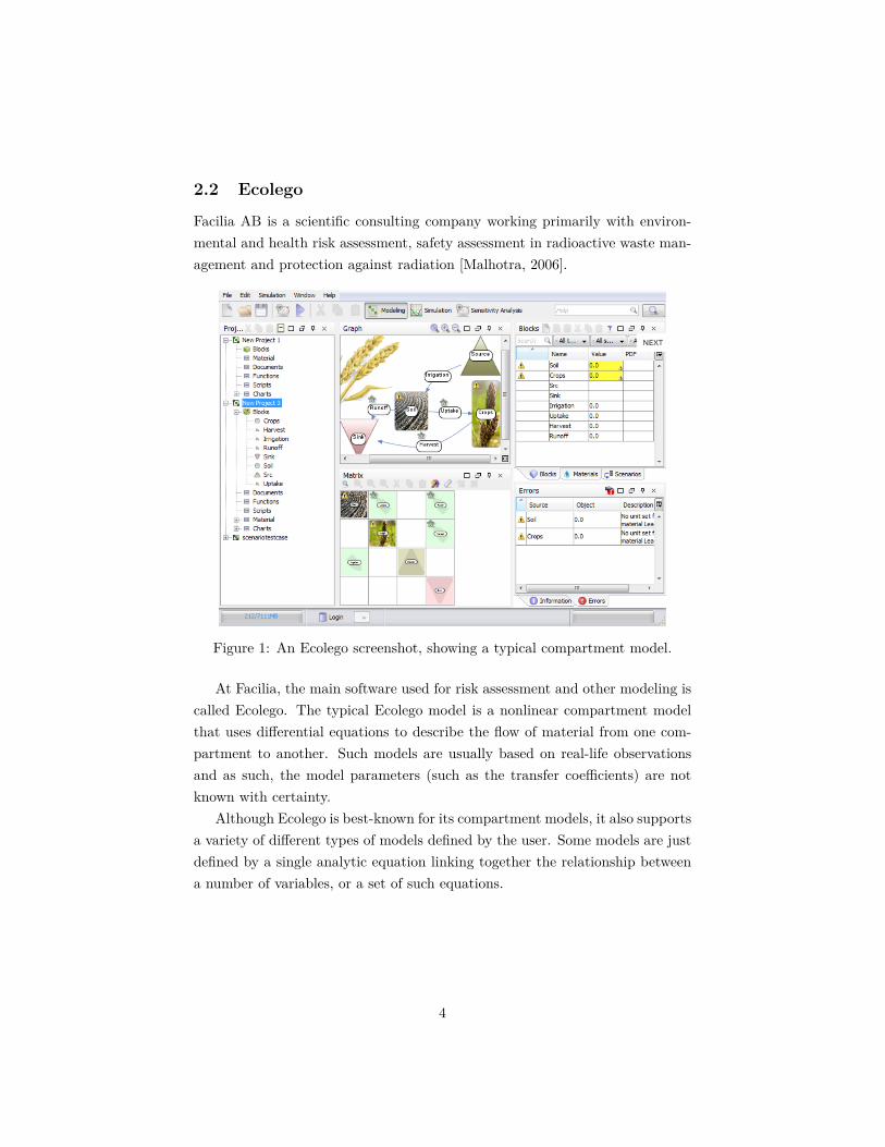
2.2 EcolegoFacilia AB is a scientific consulting company working primarily with environ-mental and health risk assessment, safety assessment in radioactive waste man-agement and protection against radiation [Malhotra, 2006].

Figure 1: An Ecolego screenshot, showing a typical compartment model.

At Facilia, the main software used for risk assessment and other modeling iscalled Ecolego. The typical Ecolego model is a nonlinear compartment modelthat uses differential equations to describe the flow of material from one com-partment to another. Such models are usually based on real-life observationsand as such, the model parameters (such as the transfer coefficients) are notknown with certainty.

Although Ecolego is best-known for its compartment models, it also supportsa variety of different types of models defined by the user. Some models are justdefined by a single analytic equation linking together the relationship betweena number of variables, or a set of such equations.

4

2.3 Statistical approachesCurrently, Ecolego is not able to give probability distributions of the parameterswithin its model when only some measurements of the model output are known.The objective of this thesis is to implement an algorithm that would providethis functionality. The problem can be phrased like this:

Given an Ecolego model M and a vector output y, what is the probabilitydistributions of the parameters θ that produced y?

In traditional frequentist statistics, probability is defined as the number ofsuccesses versus the number of trials as the number of trials approaches infinity.In other words, it is the limit:

limnTrials→∞

nSuccessesnTrials

This interpretation may not always be useful, for example when it is mean-ingless to speak of more than one trial (for example, what is the probabilitythat a candidate will win elections in a given year?). In particular, it is hardto apply the definition when finding probability distributions of model param-eters. A frequentist statistician could give confidence intervals of a parameter,but those will not provide the same amount of information as a probability dis-tribution and is less suitable for this task due to the unintuitive understandingof probability.

Bayesian statistics provide a better approach to the problem for at least tworeasons:

1. The interpretation of probability is more in line with the common senseunderstanding of what probability means (a measure of uncertainty) .

2. The Bayesian framework allows the incorporation of a priori knowledgethrough Bayes’ theorem (see Equation 1 in the next section). Such in-formation can be gathered in multiple ways, including but not limitedto:

• Expert knowledge, for example from published research on similarproblems.

5

• Experiments on the problem itself, possibly performed using differenta priori knowledge in order to generate posteriors that can be usedas a priori information in the next iteration.

• Reasonable guesses and assumptions (for example, assuming that thenumber of elements in a set can neither be negative nor exceed someparticularly high number).

Another reason for choosing the Bayesian approach is that it provides a goodframework for Markov Chain Monte Carlo methods (see next section). Withoutthis framework, solving the problem in an precise manner would be hard orimpossible.

6

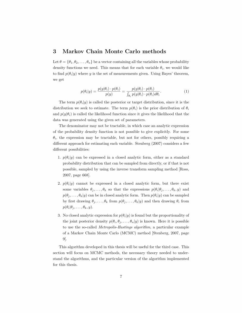
3 Markov Chain Monte Carlo methodsLet θ = {θ1, θ2, . . . , θn} be a vector containing all the variables whose probabilitydensity functions we need. This means that for each variable θi, we would liketo find p(θi|y) where y is the set of measurements given. Using Bayes’ theorem,we get

p(θi|y) = p(y|θi) · p(θi)p(y) = p(y|θi) · p(θi)�

θip(y|θi) · p(θi)dθi

. (1)

The term p(θi|y) is called the posterior or target distribution, since it is thedistribution we seek to estimate. The term p(θi) is the prior distribution of θi

and p(y|θi) is called the likelihood function since it gives the likelihood that thedata was generated using the given set of parameters.

The denominator may not be tractable, in which case an analytic expressionof the probability density function is not possible to give explicitly. For someθi, the expression may be tractable, but not for others, possibly requiring adifferent approach for estimating each variable. Stenberg (2007) considers a fewdifferent possibilities:

1. p(θi|y) can be expressed in a closed analytic form, either as a standardprobability distribution that can be sampled from directly, or if that is notpossible, sampled by using the inverse transform sampling method [Ross,2007, page 668].

2. p(θi|y) cannot be expressed in a closed analytic form, but there existsome variables θj , . . . , θk so that the expressions p(θi|θj , . . . , θk, y) andp(θj , . . . , θk|y) can be in closed analytic form. Then p(θi|y) can be sampledby first drawing θj , . . . , θk from p(θj , . . . , θk|y) and then drawing θi fromp(θi|θj , . . . , θk, y).

3. No closed analytic expression for p(θi|y) is found but the proportionality ofthe joint posterior density p(θi, θj , . . . , θn|y) is known. Here it is possibleto use the so-called Metropolis-Hastings algorithm, a particular exampleof a Markov Chain Monte Carlo (MCMC) method [Stenberg, 2007, page9].

This algorithm developed in this thesis will be useful for the third case. Thissection will focus on MCMC methods, the necessary theory needed to under-stand the algorithms, and the particular version of the algorithm implementedfor this thesis.

7

3.1 Markov chainsA Markov chain X is a sequence of random variables that fulfills the Markov

property; meaning that each variable in the sequence is dependent only on theprevious variable. Borrowing notation from Konstantopoulos (2009), this meansthat if X = {Xn, n ∈ T} where T is a subset of the integers, then X is a Markovchain if and only for all n ∈ Z+ and all mi in the state space of X, we have that

P (Xn+1 = mi+1|Xn = mn, . . . , X0 = m0) = P (Xn+1 = mi+1|Xn = mn). (2)

Thus the future process of a Markov chain is independent of its past process[Konstantopoulos, 2009]. Assuming that X has an infinite state space, thetransition kernel of X, P (Xt+1 = mi+1|P (Xt) = mt), defines the probabilitythat the Markov chain goes from one particular state to another. If the transitionkernel is not dependent on t, then X is considered time-homogeneous [Martinezand Martinez, 2002, page 429]. In this thesis, we are only interested in time-homogeneous Markov chains.

The stationary distribution of a Markov chain X is a vector π so that thetime spent in a state Xj converges to πXj after a sufficient number of iterations,independently of the initial value of X. A Markov chain that is positive recurrent

(meaning that from any given state mi, it will travel to state mj in a finitenumber of steps with probability 1) and aperiodic

1 is considered ergodic. Alltime-homogeneous ergodic Markov chains have a unique stationary distribution[Konstantopoulos, 2009].

3.2 Markov Chain Monte Carlo MethodsThe idea behind MCMC methods is to generate a Markov chain with a sta-tionary distribution that equals the posterior probability density function inEquation 1. As proved for example in [Billingsley, 1986], a Markov chain isguaranteed to converge to its stationary distribution after a sufficient numberof steps m (called the burn-in period). This can be used to find the mean ofthe posterior p(θi|y) whose corresponding Markov chain is denoted by X, bycalculating

1The period of a state mi is the greatest common divisor of all numbers n so that it ispossible to return to mi in finite steps. A Markov chain is aperiodic if every state in its statespace has period equal to one [Konstantopoulos, 2009].

8

X̄ = 1n − m

n�

t=m+1Xt (3)

where n is the number of steps taken in the Markov chain. Similar equationscan be used to calculate any statistical properties of interest of the posterior,such as its moments or quantiles. For example, in order to find the variance ofthe posterior, we calculate the following [Martinez and Martinez, 2002]:

1n − m − 1

n�

t=m+1(Xt − X̄)2 (4)

It is important to keep in mind that even though sampling in this mannerfrom X being for all intents and purposes the same as sampling from the trueposterior, any consecutive values of X are nevertheless correlated by the natureof Markov chains. In order to minimize this effect when sampling, one can takeevery kth value from X where k is a sufficiently high number. This method iscalled thinning and is suggested by [Gelman et al., 2004, page 395].

The reminder of this subsection will explain different MCMC methods togenerate Markov chains with stationary distributions equal to the probabilitydensity function of interest, ending with the adaptive Metropolis-within-Gibbsalgorithm which is of main interest for this thesis.

3.2.1 Gibbs sampling

The Gibbs sampling algorithm is used to estimate the posterior of each param-eter θi when it is possible to sample from the full conditional distributions ofeach of them, i.e. p(θi|θ−i) (where θ−i is every parameter except θi). In otherwords, we generally expect p(θi|θ−i) to be a closed analytic expression for eachi. The algorithm works as follows (as described by Jing [2010] and others):

The Gibbs sampling algorithm

1. Initialize the values of each variable θi so that θ0 = {θ

01, . . . , θ

0k}. This can

be done by sampling from the prior distributions on the variables.

2. For iteration k from 1 to N , let θk = {p(θk

1 |θk−1−1 ), . . . , p(θk

n|θk−1−n )}

3. Return {θ0, . . . , θ

N }.

9

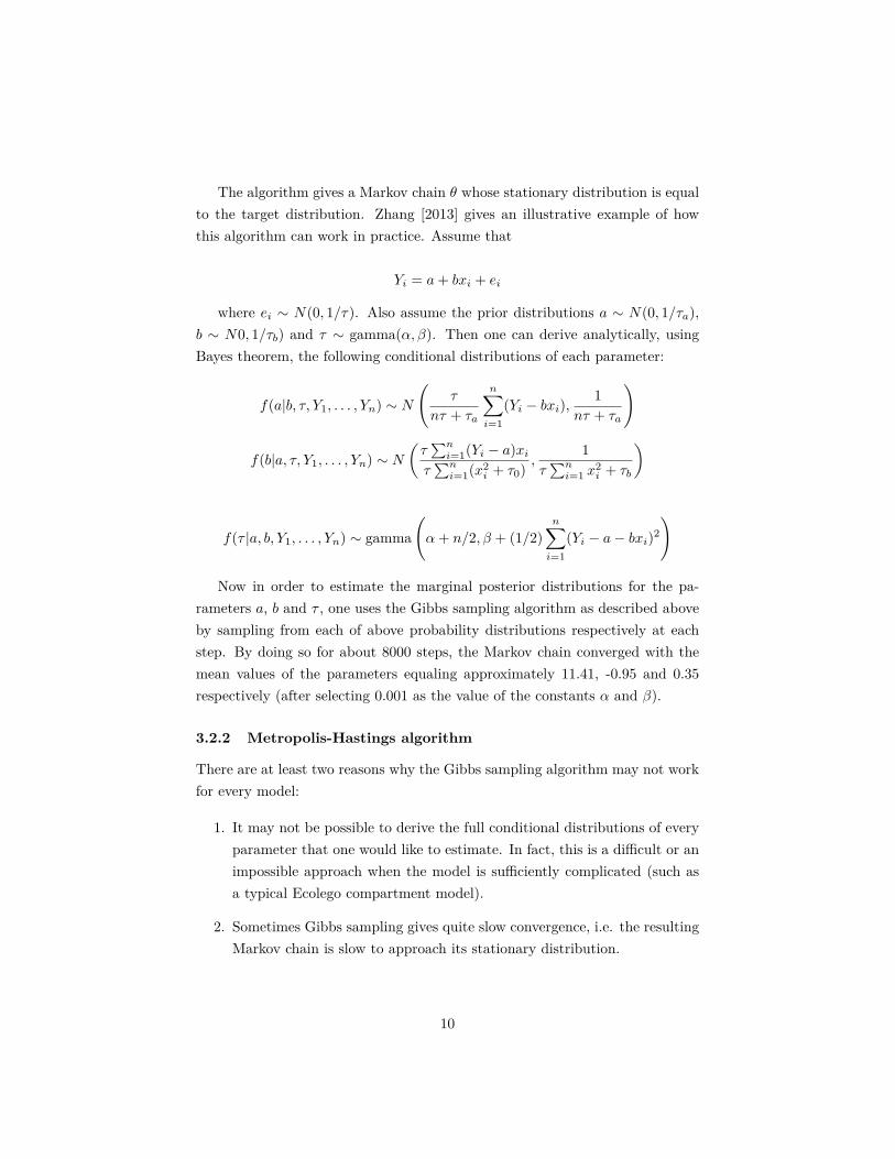
The algorithm gives a Markov chain θ whose stationary distribution is equalto the target distribution. Zhang [2013] gives an illustrative example of howthis algorithm can work in practice. Assume that

Yi = a + bxi + ei

where ei ∼ N(0, 1/τ). Also assume the prior distributions a ∼ N(0, 1/τa),b ∼ N0, 1/τb) and τ ∼ gamma(α, β). Then one can derive analytically, usingBayes theorem, the following conditional distributions of each parameter:

f(a|b, τ, Y1, . . . , Yn) ∼ N

�τ

nτ + τa

n�

i=1(Yi − bxi),

1nτ + τa

�

f(b|a, τ, Y1, . . . , Yn) ∼ N

�τ

�ni=1(Yi − a)xi

τ�n

i=1(x2i + τ0) ,

1τ

�ni=1 x

2i + τb

�

f(τ |a, b, Y1, . . . , Yn) ∼ gamma�

α + n/2, β + (1/2)n�

i=1(Yi − a − bxi)2

�

Now in order to estimate the marginal posterior distributions for the pa-rameters a, b and τ , one uses the Gibbs sampling algorithm as described aboveby sampling from each of above probability distributions respectively at eachstep. By doing so for about 8000 steps, the Markov chain converged with themean values of the parameters equaling approximately 11.41, -0.95 and 0.35respectively (after selecting 0.001 as the value of the constants α and β).

3.2.2 Metropolis-Hastings algorithm

There are at least two reasons why the Gibbs sampling algorithm may not workfor every model:

1. It may not be possible to derive the full conditional distributions of everyparameter that one would like to estimate. In fact, this is a difficult or animpossible approach when the model is sufficiently complicated (such asa typical Ecolego compartment model).

2. Sometimes Gibbs sampling gives quite slow convergence, i.e. the resultingMarkov chain is slow to approach its stationary distribution.

10

Fortunately there is an algorithm that only requires knowing the target dis-tribution to a constant of proportionality; the Metropolis algorithm [Metropoliset al., 1953]. The algorithm is very general since by Bayes Theorem, we doknow the proportionality of the target distribution as long as we know its priordistribution and the likelihood function. The description below of the algorithmis mostly due to Martinez and Martinez [2002].

The Metropolis algorithm

1. As in the Gibbs sampling algorithm, initialize the values of each variableθi so that θ

0 = {θ01, . . . , θ

0k}. In this thesis, it will be done by sampling

from the prior distributions on the variables.

2. For iteration k from 1 to N :

(a) Define a candidate value ck = q(θk−1) where q is a predefined pro-posal function.

(b) Generate a value U from the uniform (0,1) distribution.

(c) Calculate C = min�1, π(ck)/π(θk−1)

�where π is a function propor-

tional to the target distribution (i.e. the likelihood function timesthe prior of θk).

(d) If C > U , set θk+1 equal to ck. Otherwise set θ

k+1 = θk−1.

3. Return {θ0, . . . , θ

N }.

The reason that the target distribution only needs to be known to a constantof proportionality is that in the expression on the right side of the equation instep 2-c, any constants cancel out. Thus the intractable integral in Equation1 does not need to be known. To prove that the samples generated using theMetropolis algorithm converges to the target distribution, one first needs toprove that sequence generated is a Markov chain with a unique stationary dis-tribution, followed by proving that the stationary distribution equals the targetdistribution. For a proof, see [Gelman et al., 2004, page 290-291].

Unlike Gibbs sampling, the Metropolis algorithm requires a proposal func-tion to be defined to generate a candidate value in the Markov chain. Theoptimal choice for this proposal function depends on the problem. A commonchoice is the (multivariate) normal distribution with a specific mean and vari-ance. If the proposal function has the property that q(Y |X) = q(|X − Y |), then

11

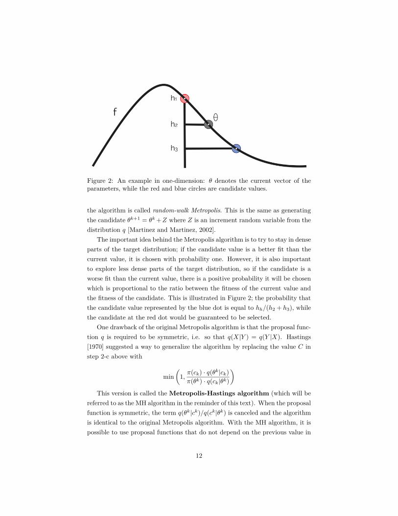
Figure 2: An example in one-dimension: θ denotes the current vector of theparameters, while the red and blue circles are candidate values.

the algorithm is called random-walk Metropolis. This is the same as generatingthe candidate θ

k+1 = θk + Z where Z is an increment random variable from the

distribution q [Martinez and Martinez, 2002].The important idea behind the Metropolis algorithm is to try to stay in dense

parts of the target distribution; if the candidate value is a better fit than thecurrent value, it is chosen with probability one. However, it is also importantto explore less dense parts of the target distribution, so if the candidate is aworse fit than the current value, there is a positive probability it will be chosenwhich is proportional to the ratio between the fitness of the current value andthe fitness of the candidate. This is illustrated in Figure 2; the probability thatthe candidate value represented by the blue dot is equal to hh/(h2 + h3), whilethe candidate at the red dot would be guaranteed to be selected.

One drawback of the original Metropolis algorithm is that the proposal func-tion q is required to be symmetric, i.e. so that q(X|Y ) = q(Y |X). Hastings[1970] suggested a way to generalize the algorithm by replacing the value C instep 2-c above with

min�

1,π(ck) · q(θk|ck)π(θk) · q(ck|θk)

�

This version is called the Metropolis-Hastings algorithm (which will bereferred to as the MH algorithm in the reminder of this text). When the proposalfunction is symmetric, the term q(θk|ck)/q(ck|θk) is canceled and the algorithmis identical to the original Metropolis algorithm. With the MH algorithm, it ispossible to use proposal functions that do not depend on the previous value in

12

the Markov chain. Such an algorithm is called an independence sampler andis implemented in this thesis along with non-independent samplers, dependingon the choice of the user. According to Martinez and Martinez [2002], runningthe independent sampler should be done with caution; it works best when theproposal function q is very similar to the target distribution.

Note that Gibbs sampling can be considered a special case of the MH al-gorithm [Gelman et al., 2004, Section 11.5]. Under that interpretation, eachnew value of θ in each iteration is considered to be a proposal with acceptanceprobability equal to one, with the “proposal function” selected appropriately.

3.2.3 Metropolis-within-Gibbs

In contrast to the MH algorithm as described above, it is possible to updateeach variable at a time in the same fashion as in Gibbs sampling. This version ofthe algorithm is called Metropolis-within-Gibbs (or Metropolis-Hastings-within-Gibbs, alternatively MH-within-Gibbs as we will call it), although this is a mis-nomer according to [Brooks et al., 2011, page 105-106] since the original paperon the Metropolis algorithm let the variables be updated one at a time. Thealgorithm works as follows:

The MH-within-Gibbs algorithm

1. As in previous algorithms, initialize the values of each variable θi so thatθ

0 = {θ01, . . . , θ

0k} (presumably by sampling from the prior distributions

on the variables).

2. For iteration k from 1 to N :

(a) For parameter i from 1 to n:

i. Define a candidate value cki = qi(θk

i ) where qi is a predefinedproposal function for parameter i.

ii. Generate a value U from the uniform (0,1) distribution.

iii. Calculate C = min�

1,π(ck

i ,θki−1)·qi(θk|ck

i ,θki−1)

π(θki )·qi(ck

i ,θki−1|θk)

�.

iv. If C > U , set θk equal to ck. Otherwise set θ

k = θk−1.

3. Return {θ0, . . . , θ

N }.

The difference here is that the parameters are updated one at a time in eachiteration, instead of either every parameter being updated in each iteration or

13

all of them remaining the same. Note that cki here is a one-dimensional num-

ber, not a vector like in the previous algorithm. The proposal functions usedfor this algorithm take a single argument, not a whole vector of parameters asbefore, and return a single argument (except in the case of an independent MH-within Gibbs sampler, in which case they take no argument). Thus π

�θ

ki−1|θk

�

means the full probability density functions with its arguments being the can-didate value of the given parameter and the other parameters from the currentiteration.

A possible advantage of the MH-within-Gibbs algorithm over the ordinaryMH algorithm is that the proposal functions are one-dimensional, so it is easierto find one and apply it (for example, the normal probability density functioncan work fine for many instances). The algorithm is also more flexible since itallows for multiple proposal functions (in fact, one for each parameter), althoughthis adds to its complexity since the user will need to specify more parameters.

3.2.4 Adaptive Metropolis-within-Gibbs

As explained before, it can be difficult to choose the proposal functions neededfor the MH-within-Gibbs algorithm. Even though one uses something straight-forward like the normal density with its mean equaling the previous value in theiteration (i.e. a random-walk Metropolis), one will still need to choose its vari-ance. This can affect how fast the Markov chain will converge to the stationarydistribution. Thus it would be desirable if the algorithm could somehow do thisfor us; if not to select the proposal function itself, at least to update its parame-ters with each iteration. This is the idea behind the adaptive MH-within-Gibbsalgorithm.

In order to do this, one can look at the acceptance ratio of candidate valuesin the algorithm and use it to update the relevant parameters. According to[Brooks et al., 2011, Chapter 4], a rule of thumb specifies that the acceptancerate for each parameter should be approximately 0.44. The authors suggest thatone can update the parameters of the proposal functions so that if the acceptanceratio is lower or higher than this number, then the parameters of the proposalfunctions are updated so that it is more likely in subsequent iterations thatcandidates are accepted or rejected respectively.

In this version of the algorithm implemented in this thesis, the parametersare updated when the acceptance rate is either lower than the number 0.25 orhigher than the number 0.45. In the former case, the parameters are updated

14

so that future candidates are more likely to be accepted; when the normaldistribution is used as a proposal function, this means that the variance islowered so that the candidate value is closer to the value used in the previousiteration. In the second case, the opposite is done. When the acceptance rateis in the range [0.25, 0.45], no special action is performed. This means thatthe parameters of the proposal function are updated more seldom than in themethod suggested by Brooks et al., which may be advantageous at least for thesake of performing fewer computations.

3.3 Choice of initial valuesAs explained in the previous section, it is necessary to initialize the values ofthe parameters θ. Although the method used in this thesis is to draw fromthe prior distributions for each variable respectively, there are other methods assuggested by [Stenberg, 2007, page 10]:

• Take a value near a point estimate derived from y (Stenberg’s chosenmethod).

• Use a mode-finding algorithm like Newton-Raphson.

• Fit a normal distribution around p(θi|y) that works as a crude approxi-mation, then draw a sample.

The above methods could work fine depending on the problem and could beimplemented in future versions of the code.

3.4 Convergence checkingAs explained before, it is non-trivial to find the optimal length of the burn-inperiod, i.e. to estimate when the Markov chains have reached convergence. Itis possible to do a rough estimation by plotting the mean value of the Markovchain (see Equation 3) versus the number of iterations and try to gauge whenthe result begins to look like a horizontal line. Alternatively, there exist severalalgorithms whose output is the optimal burn-in length. Two of them weresummarized by Martinez and Martinez [2002] and they are described in thissection.

15

3.4.1 Gelman and Rubin

The Gelman and Rubin method [Gelman and Rubin, 1992] [Gelman, 1996] re-quires multiple sets of Markov chains by running the algorithm separate times.Fortunately, it is easy to generate the Markov chains simultaneously by runningthe algorithm in parallel on a multi-core processor. The idea behind the methodis that the variance within a single chain will be less than the variance in thecombined sequences if convergence has not taken place [Martinez and Martinez,2002].

Define the between-sequence variance of the chains as

B = n

k − 1

k�

i=1

�v̄i − 1

k

k�

p=1v̄p

�2

where vij denotes the jth value in the ith sequence and

v̄i = 1n

n�

j=1vij .

Now define the within-sequence variance as

W = 1k

k�

i=1s

2i

where

s2i = 1

n − 1

n�

j=1(vij − v̄i)2

.Finally, those two values are combined in the overall variance estimate

n − 1n

W + 1n

B

According to Gelman [1996], the MCMC algorithm should be run until thevalue above is lower than 1.1 or 1.2 for every parameter to be estimated [Mar-tinez and Martinez, 2002].

3.4.2 Raftery and Lewis

Unlike the Gelman and Rubin method, the Raftery and Lewis convergence al-gorithm [Raftery and Lewis, 1996] only needs a single chain. After the user

16

has determined how much accuracy they require for the target distribution, themethod can be used to find not only how many samples should be discarded(the length of the burn-in period) but also how many iterations should be runand the optimal thinning constant k.

The user is expected to provide three constants: q, r and s. This correspondsto requiring that the cumulative distribution function of the r quantile of thetarget distribution be estimated to within ±s with probability q. In return, thealgorithm returns the values M , N and k which is the burn-in period, numberof iterations and the thinning constant respectively. For the algorithm itself,see its description in [Raftery and Lewis, 1996].

Using only a single chain to assess convergence can be advantageous forseveral reasons. For example, it does not require more than one instance ofEcolego to be run at the same time and it allows the user to try differenthyperparameters for only a single chain at a time in order to determine theoptimal values. It is also possible to combine the Raftery and Lewis methodwith the Gelman and Rubin method to get a better assessment of whetherconvergence has taken place, by generating multiple chains for the Gelman andRubin method and then using the Raftery and Lewis method on each individualchain.

17

4 ImplementationThe objective of this thesis was to create an algorithm that is as general aspossible but still powerful enough to work adequately for most problems. TheGibbs sampling algorithm is a powerful technique, but since it requires knowl-edge of the conditional distributions of each variable θi, the choice was made toimplement the adaptive MH-within-Gibbs algorithm.

The algorithm was implemented using the programming language Java withwrapper classes connected to Ecolego. There were two main reasons for writingthe code in Java:

1. The codebase behind Ecolego is mainly written in Java, thus making theintegration to Ecolego much simpler.

2. Java is a popular language with a large number of mathematical libraries(such as the Apache Commons Mathematics Library), eliminating the needto write all common probability distributions from scratch.

Furthermore, Java 8 supports lambda expressions and functional program-ming, which made it easier to work with the high number of functions withinthe algorithm. Java being an object-orientated language also made it easier tostructure the software; the proposal and prior distributions were given their ownclass and can thus be initialized as objects to be used as arguments for the mainMH-within-Gibbs sampler algorithm.

The user is expected to specify a number of arguments before the algorithmcan be run:

1. The Ecolego file that the user wants to work with; the names of its param-eters of interest (given as text strings); the values and names of constants(if any); the name of the output field.

2. Real-life measurements gathered by the user (considered the vector x inMCMC literature) and the value of t (time) when each point was collected(if applicable).

3. The prior distributions of each parameter θi and the parameters of thosedistributions. The user can select between the normal distribution, thegamma distribution and the exponential distribution.

4. The proposal functions of each parameter θi and the parameters of thoseproposal functions. The normal distribution is considered to be default

18

here, but the user can also choose the gamma or the exponential distribu-tion. For each proposal function, the user should also specify if they aresupposed to be independent (as in the independence sampler) or depen-dent on the last sample generated (as in random-walk Metropolis).

5. The number of iterations and the length of the burn-in period. After thealgorithm has been run, convergence checking is performed and the usercan see if suitable values were selected for those parameters.

6. An estimate of the error in the data, σ2. If not specified, σ is given the

default value 1.

7. A flag that denotes how the likelihood function is calculated. The optionsare normal likelihood and log-normal likelihood. Let xi be the measure-ment at time point xi (assuming that there exist n measurements) andlet v be a vector of the current values of θ so that y(v|ti) is the output ofthe model with the values of the parameters equal to v at time point t1.Then the normal likelihood is defined as

exp�

−n�

i=1

(xi − y(v|ti))2

2σ2

�

and the log-normal likelihood is

exp

−n�

i=1

�log(xi) − log (y(v|ti))2

�

2σ2

.

Thus the value of the likelihood function is in both cases maximal when theerror is zero, as it should be. The log-normal likelihood is more appropriatewhen the values of the measurements are extremely high or low (or both)such as in the case of the exponential model in Section 5.1.

8. A flag that denotes if the user wants to run the adaptive version of theMH-within-Gibbs algorithm or not.

In order to calculate the likelihood function for each parameter at each iter-ation, an update is sent to Ecolego with the new values of the parameters beforethe Ecolego model is executed. The result is then compared to the values of themeasurements. Running Ecolego models is relatively time-consuming compared

19

to other operations within the algorithm; it should be considered the bottle-neck of the implementation. Therefore, there is a tradeoff between the speedand accuracy of the results which needs to be handled carefully. However, fu-ture versions of Ecolego may be able to perform faster which could hopefullyminimize the impact of this problem.

The algorithm supports an unlimited number of variables to be estimatedand besides the three variations of prior densities and proposal functions offeredas options, the user can add their own with minor code modifications if theycan specify them programmatically. However, the user will need to specify theparameters of the prior probability densities.

In addition to this, the Galman and Rubin convergence test as described inthe previous section was implemented in a Java method. The user is expected toprovide the number of iterations that they expect to be optimal for the chainsthat have already been generated. The algorithm will then return a singlenumber that gives a measure of the convergence.

20

5 Experiments and results

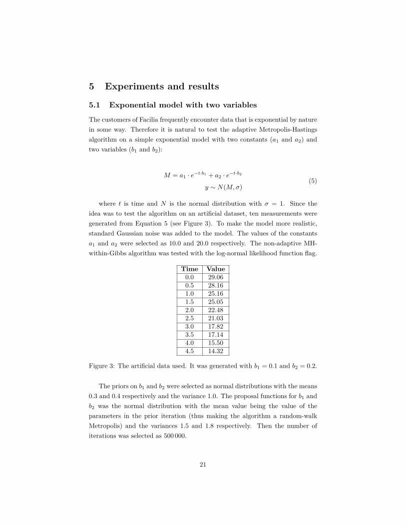
5.1 Exponential model with two variablesThe customers of Facilia frequently encounter data that is exponential by naturein some way. Therefore it is natural to test the adaptive Metropolis-Hastingsalgorithm on a simple exponential model with two constants (a1 and a2) andtwo variables (b1 and b2):

M = a1 · e−t·b1 + a2 · e

−t·b2

y ∼ N(M, σ)(5)

where t is time and N is the normal distribution with σ = 1. Since theidea was to test the algorithm on an artificial dataset, ten measurements weregenerated from Equation 5 (see Figure 3). To make the model more realistic,standard Gaussian noise was added to the model. The values of the constantsa1 and a2 were selected as 10.0 and 20.0 respectively. The non-adaptive MH-within-Gibbs algorithm was tested with the log-normal likelihood function flag.

Time Value

0.0 29.060.5 28.161.0 25.161.5 25.052.0 22.482.5 21.033.0 17.823.5 17.144.0 15.504.5 14.32

Figure 3: The artificial data used. It was generated with b1 = 0.1 and b2 = 0.2.

The priors on b1 and b2 were selected as normal distributions with the means0.3 and 0.4 respectively and the variance 1.0. The proposal functions for b1 andb2 was the normal distribution with the mean value being the value of theparameters in the prior iteration (thus making the algorithm a random-walkMetropolis) and the variances 1.5 and 1.8 respectively. Then the number ofiterations was selected as 500 000.

21

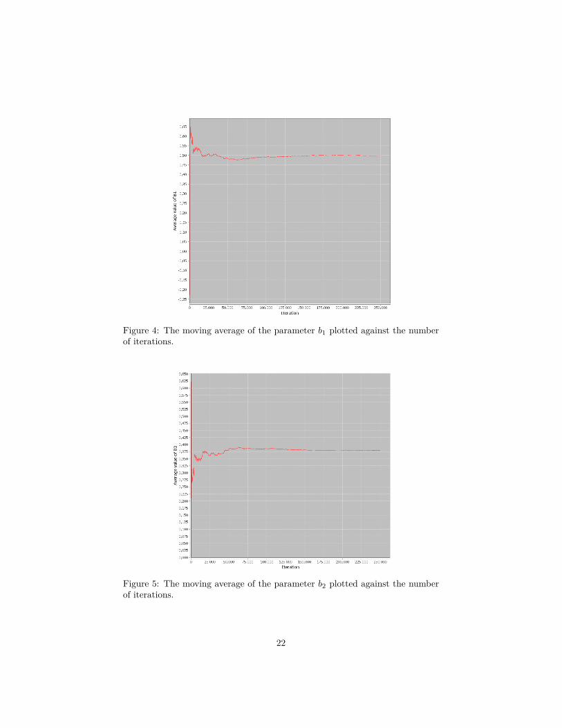
Figure 4: The moving average of the parameter b1 plotted against the numberof iterations.

Figure 5: The moving average of the parameter b2 plotted against the numberof iterations.

22

Figure 6: A histogram of the parameter b1.

Figure 7: A histogram of the parameter b2.

Observing Figures 4 and 5, it appears that the burn-in period ends roughlyat 100 000 iterations. The algorithm was run ten different times so that the

23

Gelman and Rubin convergence test could be performed with 100 000 as thenumber of iterations. This returned a number between 1.0 and 1.1, suggestingthat convergence will take place after at most this number of iterations.

The average values of the parameters b1 and b2 as computed with Equation3 were found to be 0.3170 and 0.1830 respectively. This is in line with expecta-tions; the values that were chosen to generate the test data were 0.2 and 0.1, butthe prior distributions had mean 0.4 and 0.3 respectively. Therefore we wouldexpect the values of the parameters as returned by the algorithm to be some-where in between those two lower and upper bounds. Also, the histograms ofthe parameters in Figures 6 and 7 roughly resemble the log-normal distribution,which is also what we would expect from an exponential model with normaldistributions chosen as priors.

5.2 Simple linear model with three parametersThe next model was even simpler, but with three parameters. The objectivewith this experiment was to compare the adaptive MH-within-Gibbs and thenon-adaptive MH-within-Gibbs algorithms and to see if correct results wereachieved in both cases.

The model is defined as follows:

y = (2 · a + b − c) · t

where the parameters a, b and c were to be estimated given the measurements

t y

0.0 0.01.0 5.02.0 10.03.0 15.04.0 20.05.0 25.06.0 30.07.0 35.0

which means that 2a + b − c should presumably equal 5. Each variable wasgiven the normal distribution as a prior distribution with variance 1 and means

24

3, 4 and 5 respectively. Since [a, b, c] = [3, 4, 5] solves the equation, doing asimple point estimate should return those values for the parameters. Thereforeit was interesting to see if the MH-within-Gibbs and adaptive MH-within-Gibbsalgorithms returned the same values. Both options were tested and the resultsare shown in the following figures. Note: the normal likelihood function wasused in both cases.

Figure 8: The moving average of the parameter a plotted against the numberof iterations.

Figure 9: The moving average of the parameter b plotted against the numberof iterations.

25

Figure 10: The moving average of the parameter c plotted against the numberof iterations.

Figure 11: The histogram of the parameter a.

26

Figure 12: The histogram of the parameter b.

Figure 13: The histogram of the parameter c.

Figures 8, 9 and 10 indicate that the adaptive MH-within-Gibbs algorithmconverges faster than the non-adaptive algorithm, which is as expected. The

27

histograms suggest that the posterior is normally distributed, which is expectedfor a linear model with normal priors.

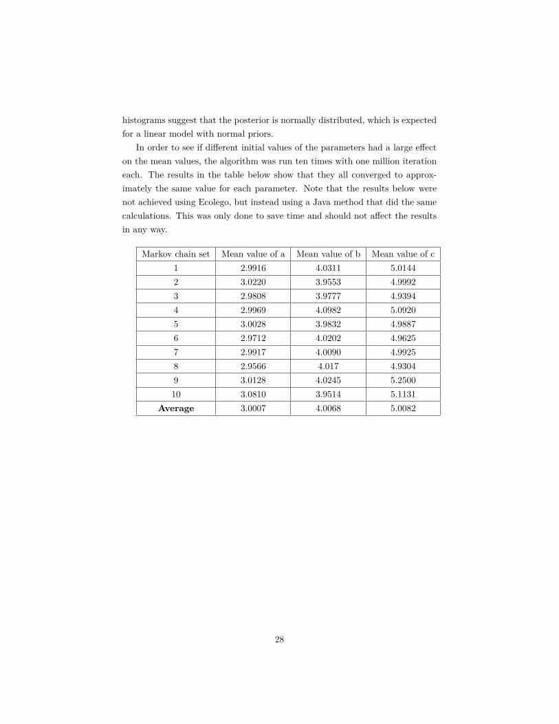
In order to see if different initial values of the parameters had a large effecton the mean values, the algorithm was run ten times with one million iterationeach. The results in the table below show that they all converged to approx-imately the same value for each parameter. Note that the results below werenot achieved using Ecolego, but instead using a Java method that did the samecalculations. This was only done to save time and should not affect the resultsin any way.

Markov chain set Mean value of a Mean value of b Mean value of c1 2.9916 4.0311 5.01442 3.0220 3.9553 4.99923 2.9808 3.9777 4.93944 2.9969 4.0982 5.09205 3.0028 3.9832 4.98876 2.9712 4.0202 4.96257 2.9917 4.0090 4.99258 2.9566 4.017 4.93049 3.0128 4.0245 5.250010 3.0810 3.9514 5.1131

Average 3.0007 4.0068 5.0082

28

6 ConclusionsNo number of experiments can possibly prove if the algorithm implemented inthis thesis is working correctly (although it would only take one experiment toprove that it is working incorrectly). However, the results gathered by testingthe algorithm on the two models in the previous section were as expected bysome metrics:

1. The Markov chains do in all cases converge, which is visible by analyzingthe mean values of the parameters plotted against the number of iterationsand by running the Gelman and Rubin convergence test on multiple setsof chains.

2. The histograms of the variables imitate the probability distributions thatwere expected from the models with the given priors: the normal distri-bution and the log-normal distribution.

3. The mean value of the parameters were in the same range as expected.However, other statistical attributes of the samples (such as variance) werenot gathered or analyzed.

Hence the conclusion is that the algorithm is likely working properly on atleast relatively simple non-hierarchical models, although further testing shouldbe done with different types of prior distributions and different types of models.

The advantage of the adaptive MH-within-Gibbs algorithm over the non-adaptive version seems to be the speed of convergence. It does not seem toaffect the results, which is as expected.

29

7 Future workVarious improvements and additions to the algorithm should be implementedin the future:

1. The Raftery and Lewis convergence checking algorithm would be a niceadditional convergence checking algorithm. If it were to be implemented,it would not be necessary to run multiple sets of chains in order to assessconvergence.

2. The user of the algorithm should be able to select between multiple meth-ods to initialize the values of the parameters, not just sampling from theprior distributions. Ideally, multiple sets of chains should be computedin parallel using each method and the convergence of each chain shouldbe assessed in order to see which method worked best for the model inquestion.

3. The user should not have to specify the length of the burn-in period them-selves. Currently, the value that the user provides is used for convergencechecking and then the algorithm accepts or rejects the value depending onthe results. Instead, convergence checking should be performed at regularintervals, and after which convergence is determined to have taken place,all previous values in the chains can be thrown away and future iterationscan be computed as under normal circumstances.

4. A higher number of probability distributions should be offered to be usedas prior distributions and proposal distributions.

5. The measurement error could be treated as a variable to be estimated.For several applications, this could be useful.

30

8 BibliographyBillingsley, P. (1986). Probablity and Measure. Wiley series in probability and

mathematical statistics. Wiley.

Brooks, S., A. Gelman, G. Jones, and X.-L. Meng (2011). Handbook of Markov

Chain Monte Carlo. Chapman & Hall/CRC Handbooks of Modern StatisticalMethods. Chapman & Hall/CRC.

Calvetti, D., R. Hageman, and E. Somersalo (2006). Large-scale bayesian pa-rameter estimation for a three-compartment cardiac metabolism model duringischemia. Inverse Problems 22 (5).

Gelman, A. (1996). Inference and monitoring convergence. In W. R. Gilks,S. Richardson, and D. T. Spiegelhalter (Eds.), Markov Chain Monte Carlo in

Practice, pp. 131–143. Chapman & Hall/CRC.

Gelman, A., J. B. Carlin, H. S. Stern, and D. B. Rubin (2004). Bayesian Data

Analysis (2 ed.). Texts in Statistical Science. Chapman & Hall/CRC.

Gelman, A. and D. Rubin (1992). Inference from iterative simulation usingmultiple sequences (with discussion). Statistical Science 7, 457–511.

Hastings, W. (1970). Monte Carlo sampling methods using Markov chains andtheir applications. Biometrika.

Jacquez, J. A. (1996). Compartmental Analysis in Biology and Medicine (3 ed.).Cambridge University Press.

Jacquez, J. A. (1999). Modeling with Compartments (1 ed.). BioMedware, USA.

Jing, L. (2010). Hastings-within-Gibbs algorithm: Introduction and appli-cation on hierarchical model. http://georglsm.r-forge.r-project.org/

site-projects/pdf/Hastings_within_Gibbs.pdf. Online; accessed 2016-05-01.

Konstantopoulos, T. (2009). Introductory lecture notes on Markov Chains andrandom walks. http://www2.math.uu.se/~takis/L/McRw/mcrw.pdf. [On-line; accessed 2016-03-30].

Malhotra, M. (2006). Bayesian updating of a non-linear ecological risk assess-ment model. Master’s thesis, Royal Institute of Technology.

31

Martinez, W. L. and A. R. Martinez (2002). Computational Statistics Handbook

with MATLAB. Chapman & Hall/CRC.

Metropolis, N., A. Rosenbluth, M. Rosenbluth, A. Teller, , and Teller (1953).Equation of state calculations by fast computing machines. Journal of Chem-

ical Physics.

Raftery, A. and M. Lewis (1996). Implementing mcmc. In W. R. Gilks,S. Richardson, and D. T. Spiegelhalter (Eds.), Markov Chain Monte Carlo in

Practice, pp. 115–130. Chapman & Hall/CRC.

Ross, S. M. (2007). Introduction to probability models (9 ed.). Academic Press.

Seber, G. A. F. and C. J. Wild (2003). Nonlinear Regression (1 ed.). Wileyseries in probability and mathematical statistics. Wiley.

Stenberg, K. (2007). Bayesian models to enhance parameter estimation of fi-nancial assets – proposal and evaluation of probabilistic methods. Master’sthesis, Stockholm University.

Zhang, H. (2013). An example of Bayesian analysis through theGibbs sampler. http://www.stat.purdue.edu/~zhanghao/MAS/handout/

gibbsBayesian.pdf. Online; accessed 2016-03-15.

32