MODEL-BASED NETWORKED CONTROL SYSTEMS – NECESSARY …

MODEL-BASED NETWORKED CONTROL SYSTEMS – NECESSARY AND SUFFICIENT CONDITIONS FOR

STABILITY

Luis A. Montestruque, Panos J. Antsaklis

University of Notre Dame, Notre Dame, IN 46556, U.S.A. Department of Electrical Engineering

fax: (574) 631-4393 e-mail: {lmontest, pantsakl}@nd.edu

Keywords: control over networks, stabilizability, minimum feedback information, hybrid systems.

Abstract In this paper the control of a continuous linear plant where the state sensor is connected to a linear controller/actuator via a network is addressed. The work focuses on reducing the network usage using knowledge of the plant dynamics. Specifically, the controller uses an explicit model of the plant that approximates the plant dynamics and makes possible the stabilization of the plant even under slow network conditions. Necessary and sufficient conditions for stability are derived in terms of the update time h and the parameters of the plant and of its model. The deterioration of behavior when either h or the modeling error increase is explicitly shown.

1 Introduction The use of networks as a media to interconnect the different components in an industrial control system is rapidly increasing. For example in geographically distributed systems the number and/or location of different subsystems to control make the use of single wires to interconnect the control system prohibitively expensive. In addition, the flexibility and ease of maintenance of a system using a network to transfer information is appealing. Systems designed in this manner allow for easy modification of the control strategy by rerouting signals, having redundant systems that can be activated automatically when component

failure occurs, and in general they allow having a high level supervisor control over the entire plant.

A network introduces bandwidth restrictions. To overcome these bandwidth constraints several approaches have been proposed. In [6] Brockett introduces the notion of minimum attention control that attempts to reduce the time and state feedback dependence of the control law. This can be viewed as a tradeoff between open loop and closed loop control.

Bauer et al. analyze the problem on a network with random delays in [3]. The paper proposes the use of a Smith predictor in a discrete framework to eliminate the delay induced by the network. The Smith predictor uses knowledge about the plant to propagate forward the delayed information from the sensor and make it accessible to the controller.

In [24, 21], Walsh et al. introduces the notion of maximal allowable transfer interval, MATI, to place an upper bound on the time between transfers of information from the sensor to the controller. In this case the controller is designed without taking the network into account, a desirable feature. However, serious behavior degradation can result if the MATI is too large and the network slow.

In [5] Beldiman, Walsh and Bushnell extend the results in [24] to include a state predictor, for LTI systems, to estimate the state in between updates.

In [20] synthesis and existence of a networked optimal controller for nonstationary linear parameter varying (LPV) systems are shown.

Other approaches include the study of networked systems with transport delays [13], and under noise

Luis A. Montestruque and Panos J. Antsaklis, "Model-Based Networked Control Systems-Necessary and Sufficient Conditions for Stability," Proceedings of the 10th Mediterranean Conference on Control and Automation (MED’02), Lisbon, Portugal, July 9-12, 2002.

disturbances [4, 17], quantization effects and algorithms [8, 10, 11, 16], and scheduling algorithms [9, 18, 12, 22, 23].

2 A State Feedback Networked Control System

It is clear that the reduction of bandwidth necessitated by the communication network in a networked control system is a major concern. This can perhaps be addressed by two methods: the first is to reduce the number of data packet exchanges between the sensor and the controller/actuator. The second method is to compress or reduce the size of the data transferred at each transaction.

Actually deployed and popular networks in the industry include CAN bus, PROFIBUS, DeviceNet, ControlNet, Fieldbus Foundation, and Ethernet among others. Each of these protocols and standards has very different characteristics such as network contention resolution or scheduling schemes, transmission media, etc. Among the shared characteristics are the small transport time and big overhead (network control information included in the packet). For example, an Ethernet frame with 1 byte of data will have the same length as one with 46 bytes of data. Similarly, the CAN bus, usually associated with the DeviceNet protocol has an overhead of 47 bits or 6 bytes approximately for a maximum data size of 8 bytes. This means that data compression by reducing the size of the data transmitted has negligible effects over the overall system performance. So reducing the number of packets transmitted brings better benefits than data compression. The reduction of the number of packets transmitted through the network can translate into larger minimal transfer times between the components. It is also to be noted that any delay in an information transaction is usually due to network access contention. This translates into what has been already noted in [23]: that a sensor with a fast sampling rate can send through the network the latest data available resulting in a negligible information transfer delay. But there will still be contention in the network so that, even though the delay is small, the sensor data would not be available at all times to the

controller/actuator. This brings us again to the idea of reducing the data transfer rate as much as possible. In this manner more bandwidth will be available to allocate more resources without sacrificing stability and ultimately performance of the overall system.

We will consider the case where the controller and the actuator are combined together into a single node. That is, the network is between the sensor and the controller/actuator nodes. Assuming that the controller and the actuator physically coexist is reasonable since embedded microprocessors are usually incorporated into the actuator to process the data received by the network and execute the commands received.

In this paper we will concentrate on characterizing the transfer time between the sensor and the controller/actuator, which is the time between information exchanges. Our goal will be to identify the maximum transfer time between the sensor and the actuator while keeping the system stable. This will reduce the bandwidth required from the network and will free it for other tasks such as other control loops using the network and/or non-control information exchange. In order to increase the transfer time we will use the knowledge we have of the plant dynamics. The plant model is used at the controller/actuator side to recreate the plant behavior so that the sensor can delay sending data since the model can provide an approximation of the plant dynamics. The main idea is to perform the feedback by updating the model’s state using the actual state of the plant that is provided by the sensor. The rest of the time the control action is based on a plant model that is incorporated in the controller/actuator and is running open loop for a period of h seconds. The control architecture is shown in Figure1.

This idea of a tradeoff between open loop and closed loop control is related to the minimal attention control proposed by Brockett in [6]. One of the main differences resides in that minimal attention control makes this tradeoff in a continuous way. The resulting controller works similarly to a sampled data system. The lack of awareness of the controller of the intersampling


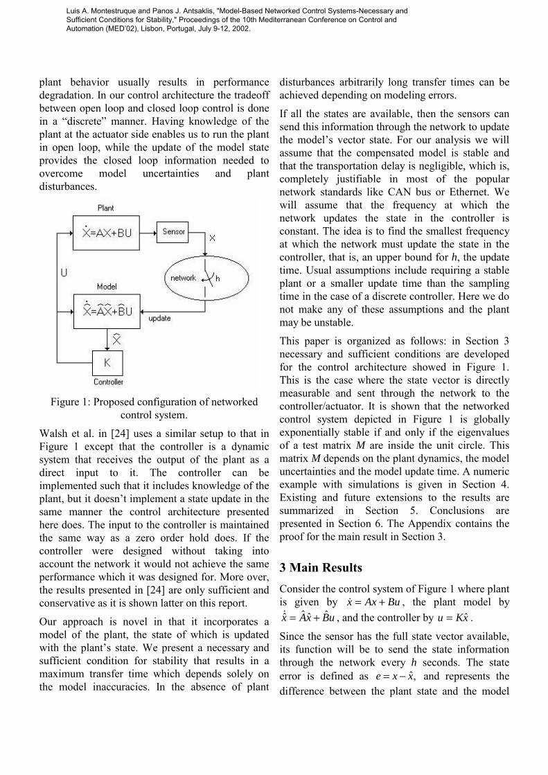
plant behavior usually results in performance degradation. In our control architecture the tradeoff between open loop and closed loop control is done in a “discrete” manner. Having knowledge of the plant at the actuator side enables us to run the plant in open loop, while the update of the model state provides the closed loop information needed to overcome model uncertainties and plant disturbances.

Figure 1: Proposed configuration of networked

control system.

Walsh et al. in [24] uses a similar setup to that in Figure 1 except that the controller is a dynamic system that receives the output of the plant as a direct input to it. The controller can be implemented such that it includes knowledge of the plant, but it doesn’t implement a state update in the same manner the control architecture presented here does. The input to the controller is maintained the same way as a zero order hold does. If the controller were designed without taking into account the network it would not achieve the same performance which it was designed for. More over, the results presented in [24] are only sufficient and conservative as it is shown latter on this report.

Our approach is novel in that it incorporates a model of the plant, the state of which is updated with the plant’s state. We present a necessary and sufficient condition for stability that results in a maximum transfer time which depends solely on the model inaccuracies. In the absence of plant

disturbances arbitrarily long transfer times can be achieved depending on modeling errors.

If all the states are available, then the sensors can send this information through the network to update the model’s vector state. For our analysis we will assume that the compensated model is stable and that the transportation delay is negligible, which is, completely justifiable in most of the popular network standards like CAN bus or Ethernet. We will assume that the frequency at which the network updates the state in the controller is constant. The idea is to find the smallest frequency at which the network must update the state in the controller, that is, an upper bound for h, the update time. Usual assumptions include requiring a stable plant or a smaller update time than the sampling time in the case of a discrete controller. Here we do not make any of these assumptions and the plant may be unstable.

This paper is organized as follows: in Section 3 necessary and sufficient conditions are developed for the control architecture showed in Figure 1. This is the case where the state vector is directly measurable and sent through the network to the controller/actuator. It is shown that the networked control system depicted in Figure 1 is globally exponentially stable if and only if the eigenvalues of a test matrix M are inside the unit circle. This matrix M depends on the plant dynamics, the model uncertainties and the model update time. A numeric example with simulations is given in Section 4. Existing and future extensions to the results are summarized in Section 5. Conclusions are presented in Section 6. The Appendix contains the proof for the main result in Section 3.

3 Main Results Consider the control system of Figure 1 where plant is given by BuAxx += , the plant model by

uBxAx ˆˆˆˆ += , and the controller by xKu ˆ= .

Since the sensor has the full state vector available, its function will be to send the state information through the network every h seconds. The state error is defined as ,x̂xe −= and represents the difference between the plant state and the model


state. The modeling error matrices BBBAAA ˆ~ andˆ~ −=−= represent the difference

between the plant and the model. Finally, the update times are kt , where htt kk =− −1 for all k. Since the model state is updated every kt seconds,

0)( =kte for ...,2,1,0=k . This resetting of the state error every update time is a key factor in our control system.

Now for ),[ 1+∈ kk ttt , we have that:

xKu ˆ=

so

+

=

xx

KBABKA

xx

ˆˆˆ0ˆ

with initial conditions )()(ˆ kk txtx =

Introducing the error )(ˆ)()( txtxte −= , it is easy to see that the dynamics of the overall system for

),[ 1+∈ kk ttt can be described by

httwithttt

txtetx

tetx

KBAKBA

BKBKAtetx

kkkk

k

k

k

=−∈∀

=

−+

−+=

++

−

11 ),,[

,0

)()()(

)()(

~ˆ~~)()(

(1)

Define now

=

)()(

)(tetx

tz , and

−+

−+=Λ

KBAKBA

BKBKA~ˆ~~ so that Equation (1) can be

rewritten as zz Λ= for ),[ 1+∈ kk ttt .

We will now express z(t) in terms of the initial condition x(t0). Then we will show under what conditions the system will be stable.

Proposition #1

The system described by Equation (1) with initial

conditions 00

0 0)(

)( ztx

tz =

= , has the following

response:

httwithttt

zI

eI

etz

kkkk

khtt k

=−∈

=

++

Λ−Λ

11

0)(

),,[

000

000

)(

Proof.

On the interval ),[ 1+∈ kk ttt , the system response is

)(0

)()()(

)( )()(k

ttktt tzetx

etetx

tz kk −Λ−Λ =

=

= (2)

Now, note that at times kt ,

=

0)(

)( kk

txtz , that is,

the error e(t) is reset to zero. We can represent this by

)(000

)( −

= kk tz

Itz

Using Equation (2) to calculate )( −ktz we obtain

)(000

)( 1−Λ

= k

hk tze

Itz

In view of (2) we have that if at time t=t0,

==

0)( 0

00

xztz is the initial condition then

0)(

2)(

1)(

)(

000

)(000

000

)(000

)()(

zeI

e

tzeI

eI

e

tzeI

e

tzetz

k

htt

khhtt

khtt

ktt

k

k

k

k

=

=

=

=

Λ−Λ

−ΛΛ−Λ

−Λ−Λ

−Λ

(3)


Now we know that heI Λ

000

is of the form

00NM

and so k

heI

Λ

000

has the form

00PM K

.

Additionally we note the special form of the initial

condition

==

0)( 0

00

xztz so that

=

=

Λ

Λ

0000

000

000

0000

0

00

xIe

I

xMxe

I

kh

kk

h

(4)

In view of Equation (4) it is clear that we can represent the system response as:

httwithttt

zI

eI

etz

kkkk

khtt k

=−∈

=

++

Λ−Λ

11

0)(

),,[

000

000

)(

(5)

♦

A necessary and sufficient condition for stability of the networked system will now be presented. For this the following definition for global exponential stability [1] is needed.

Definition #1

The equilibrium 0=z of a system described by ),( ztfz = with initial condition 00 )( ztz = is

exponentially stable at large (or globally) if there exists 0>α and for any 0>β , there exists

0)( >βk such that the solution

0)(

000 ,)(),,( 0 ttezkztt tt ≥∀≤ −−αβφ

whenever β<0z .

With this definition of stability we state the following theorem characterizing the necessary and sufficient conditions for the system described by Equation (1) to have global exponential stability

around the solution 0=z . The norm used here is the 2-norm but any other consistent norm can also be used.

Theorem #1

The system described by Equation (1) is globally exponentially stable around the solution

=

=

00

ex

z if and only if the eigenvalues of

Λ

000

000 I

eI h are strictly inside the unit circle.

Proof – See Appendix.

It can be shown (as in [15]) that the eigenvalues of

= Λ

000

000 I

eI

M h are inside the unit circle if and

only if the eigenvalues of

τττ deKBAeeeI KBAh AAhhKBA )ˆˆ(

0

)ˆˆ( )~~( +−+ ++= ∫ are

inside the unit circle. One can gain a better insight of the system by observing the structure of I. To start with, we observe that the eigenvalues of the compensated model appear in the first term of I. In that sense we can see the term

τττ deKBAee KBAh AAh )ˆˆ(

0)~~( +− +=∆ ∫ as a

perturbation over the desired eigenvalues. Even if the eigenvalues of the original plant were unstable the perturbation ∆ can be made small enough by having h and KBA ~~ + small and thus minimizing their impact over the eigenvalues of the compensated plant. We also observe that if the update time h is driven to zero, then ∆=0. Also it is possible to make ∆=0 by having a model that is exact. This agrees with the intuition that if the model has exactly the same dynamics as the plant then the system will have the desired behavior regardless of how long is the update time h.

4 Example Consider the following unstable plant (double integrator):


=

=

10

,0010

BA

We will use the state feedback controller given by Kxu = with [ ]21 −−=K .

Usually it is assumed that the actuator/controller will hold the last value received from the sensor until the next time the sensor transmits and a packet is received. Under this assumption the controller/actuator’s model acts as a zero order hold when updated. We will first analyze this situation. To do so, we will transform the plant model so that it holds the last state update presented to it by the network. So the model designed to behave as a zero order hold when updated is given by:

.00ˆ,

0000ˆ,ˆˆˆˆ

=

=+= BAuBxAx

So now we need to search for the biggest h such

that

Λ

000

000 I

eI h has its eigenvalues inside the

unit circle. In this case Λ is given by:

−−

−−=

−+

−+=Λ

2121001021210010

~ˆ~~ KBAKBABKBKA

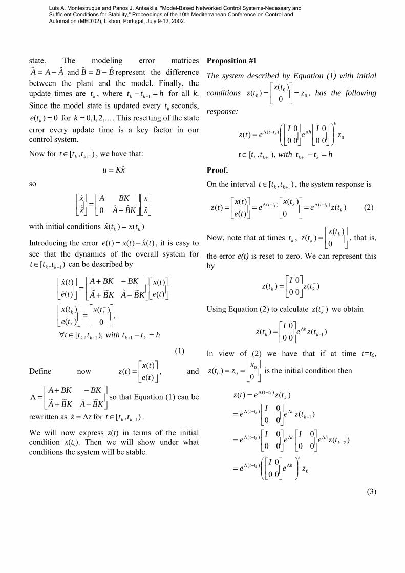
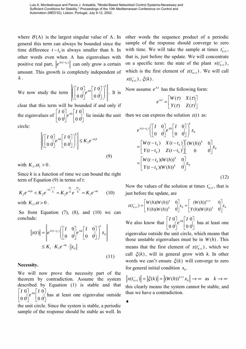
To do so we plotted the maximum eigenvalue magnitude versus the update time. The plot is shown in Figure 2.

From Figure 2 we see that the condition for stability is to have h < 1 second. In fact the test matrix M will have one eigenvalue with magnitude 1 for h=1 second. If we use the results by [23] or [24] we would have obtained that, in order to stabilize the system, we would need to have h<2.1304E-4, which is very conservative.

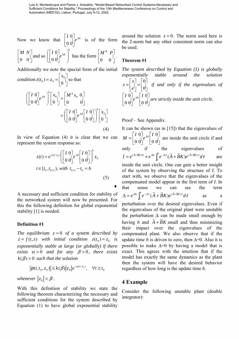
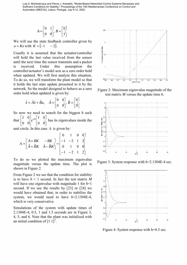
Simulations of the system with update times of 2.1304E-4, 0.5, 1 and 1.5 seconds are in Figure 3, 4, 5, and 6. Note that the plant was initialized with an initial condition of [1 1]T.

Figure 2: Maximum eigenvalue magnitude of the

test matrix M versus the update time h.

Figure 3: System response with h=2.1304E-4 sec.

Figure 4: System response with h=0.5 sec.


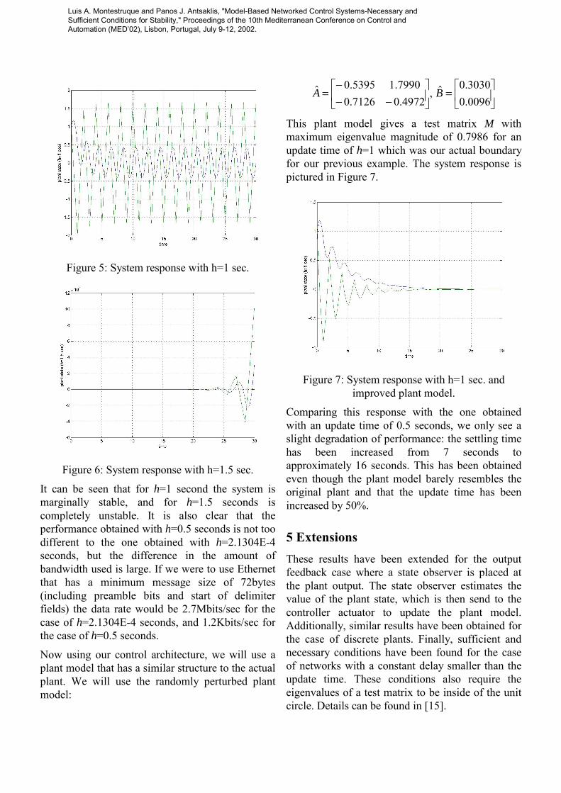
Figure 5: System response with h=1 sec.

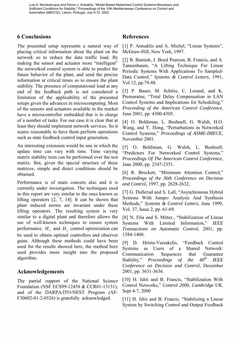
Figure 6: System response with h=1.5 sec.

It can be seen that for h=1 second the system is marginally stable, and for h=1.5 seconds is completely unstable. It is also clear that the performance obtained with h=0.5 seconds is not too different to the one obtained with h=2.1304E-4 seconds, but the difference in the amount of bandwidth used is large. If we were to use Ethernet that has a minimum message size of 72bytes (including preamble bits and start of delimiter fields) the data rate would be 2.7Mbits/sec for the case of h=2.1304E-4 seconds, and 1.2Kbits/sec for the case of h=0.5 seconds.

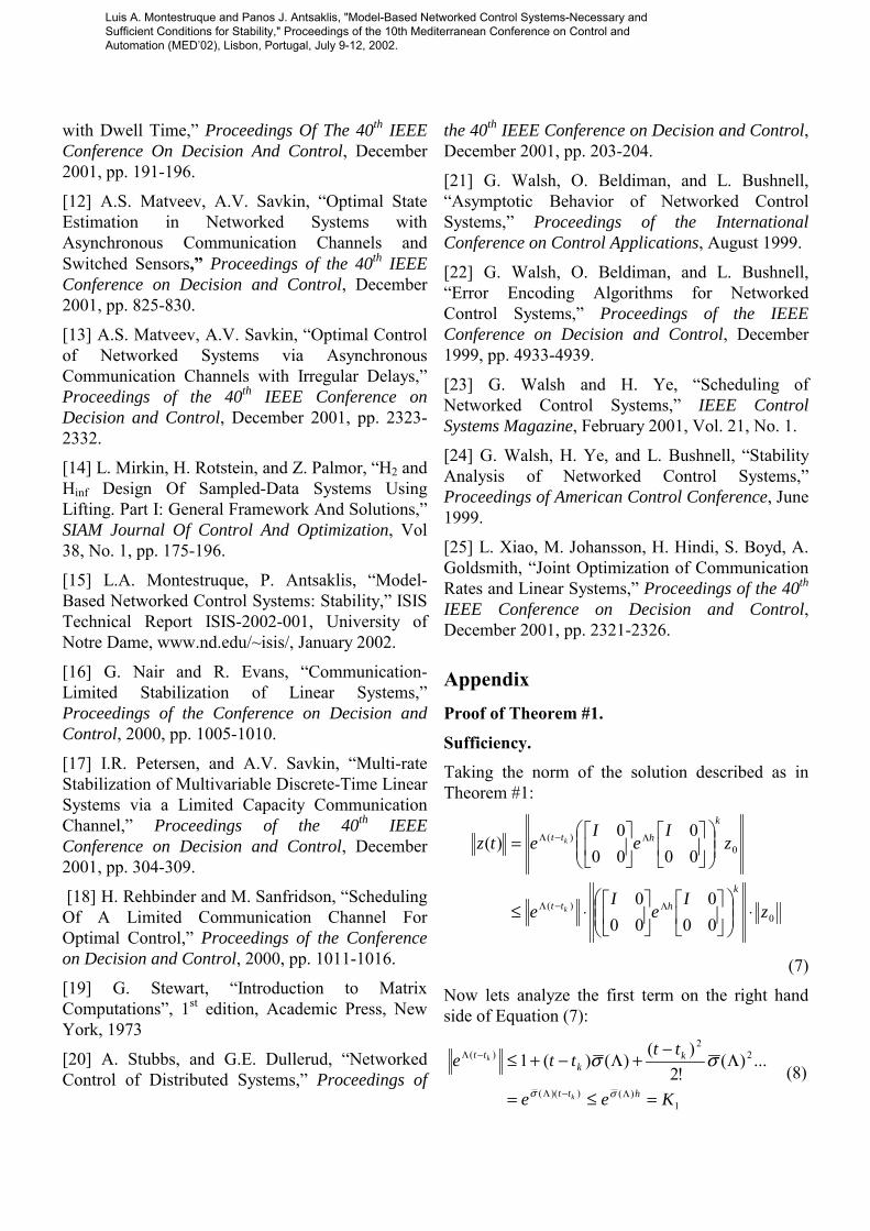
Now using our control architecture, we will use a plant model that has a similar structure to the actual plant. We will use the randomly perturbed plant model:

=

−−

−=

0096.03030.0ˆ,

4972.07126.07990.15395.0ˆ BA

This plant model gives a test matrix M with maximum eigenvalue magnitude of 0.7986 for an update time of h=1 which was our actual boundary for our previous example. The system response is pictured in Figure 7.

Figure 7: System response with h=1 sec. and

improved plant model.

Comparing this response with the one obtained with an update time of 0.5 seconds, we only see a slight degradation of performance: the settling time has been increased from 7 seconds to approximately 16 seconds. This has been obtained even though the plant model barely resembles the original plant and that the update time has been increased by 50%.

5 Extensions These results have been extended for the output feedback case where a state observer is placed at the plant output. The state observer estimates the value of the plant state, which is then send to the controller actuator to update the plant model. Additionally, similar results have been obtained for the case of discrete plants. Finally, sufficient and necessary conditions have been found for the case of networks with a constant delay smaller than the update time. These conditions also require the eigenvalues of a test matrix to be inside of the unit circle. Details can be found in [15].


6 Conclusions The presented setup represents a natural way of placing critical information about the plant on the network so to reduce the data traffic load. By making the sensor and actuator more “intelligent” the networked control system is able to predict the future behavior of the plant, and send the precise information at critical times so to ensure the plant stability. The presence of computational load at any end of the feedback path is not considered a limitation of the applicability of the presented setups given the advances in microcomputing. Most of the sensors and actuators available in the market have a microcontroller embedded that is in charge of a number of tasks. For our case it is clear that at least they should implement network services. So it seams reasonable to have them perform operations such as state feedback control input generation.

An interesting extension would be one in which the update time can vary with time. Time varying matrix stability tests can be performed over the test matrix. But, given the special structure of these matrices, simple and direct conditions should be obtained.

Performance is of main concern also and it is currently under investigation. The techniques used in this report are very similar to the ones known as lifting operators [2, 7, 14]. It can be shown that plant induced norms are invariant under these lifting operators. The resulting system is very similar to a digital plant and therefore allows the use of well-known techniques to ensure system performance. ∞H and 2H control optimization can be used to obtain optimal controllers and observer gains. Although these methods could have been used for the results showed here, the method here used provides more insight into the proposed algorithm.

Acknowledgements The partial support of the National Science Foundation (NSF ECS99-12458 & CCR01-13131), and of the DARPA/ITO-NEST Program (AF-F30602-01-2-0526) is gratefully acknowledged.

References [1] P. Antsaklis and A. Michel, “Linear Systems”, McGraw-Hill, New York, 1997.

[2] B. Bamieh, J. Boyd Pearson, B. Francis, and A. Tannenbaum, “A Lifting Technique For Linear Periodic Systems With Applications To Sampled-Data Control,” Systems & Control Letters, 1991, Vol 12, pp.79-88.

[3] P. Bauer, M. Schitiu, C. Lorand, and K. Premaratne, “Total Delay Compensation in LAN Control Systems and Implications for Scheduling,” Proceeding of the American Control Conference, June 2001, pp. 4300-4305.

[4] O. Beldiman, L. Bushnell, G. Walsh, H.O. Wang, and Y. Hong, “Perturbations in Networked Control Systems,” Proceedings of ASME-IMECE, November 2001.

[5] O. Beldiman, G. Walsh, L. Bushnell, “Predictors For Networked Control Systems,” Proceedings Of The American Control Conference, June 2000, pp. 2347-2351.

[6] R. Brockett, “Minimum Attention Control,” Proceedings of the 36th Conference on Decision and Control, 1997, pp. 2628-2632.

[7] G. Dullerud and S. Lall, “Asynchronous Hybrid Systems With Jumps- Analysis And Synthesis Methods,” Systems & Control Letters, June 1999, Vol. 37, Issue 2, pp. 61-69.

[8] N. Elia and S. Mitter., “Stabilization of Linear Systems With Limited Information,” IEEE Transactions on Automatic Control, 2001, pp. 1384-1400.

[9] D. Hristu-Varsakelis, “Feedback Control Systems as Users of a Shared Network: Communication Sequences that Guarantee Stability,” Proceedings of the 40th IEEE Conference on Decision and Control, December 2001, pp. 3631-3636.

[10] H. Ishii and B. Francis, “Stabilization With Control Networks,” Control 2000, Cambridge UK, Sept 4-7, 2000

[11] H. Ishii and B. Francis, “Stabilizing a Linear System by Switching Control and Output Feedback


with Dwell Time,” Proceedings Of The 40th IEEE Conference On Decision And Control, December 2001, pp. 191-196.

[12] A.S. Matveev, A.V. Savkin, “Optimal State Estimation in Networked Systems with Asynchronous Communication Channels and Switched Sensors,” Proceedings of the 40th IEEE Conference on Decision and Control, December 2001, pp. 825-830.

[13] A.S. Matveev, A.V. Savkin, “Optimal Control of Networked Systems via Asynchronous Communication Channels with Irregular Delays,” Proceedings of the 40th IEEE Conference on Decision and Control, December 2001, pp. 2323-2332.

[14] L. Mirkin, H. Rotstein, and Z. Palmor, “H2 and Hinf Design Of Sampled-Data Systems Using Lifting. Part I: General Framework And Solutions,” SIAM Journal Of Control And Optimization, Vol 38, No. 1, pp. 175-196.

[15] L.A. Montestruque, P. Antsaklis, “Model-Based Networked Control Systems: Stability,” ISIS Technical Report ISIS-2002-001, University of Notre Dame, www.nd.edu/~isis/, January 2002.

[16] G. Nair and R. Evans, “Communication-Limited Stabilization of Linear Systems,” Proceedings of the Conference on Decision and Control, 2000, pp. 1005-1010.

[17] I.R. Petersen, and A.V. Savkin, “Multi-rate Stabilization of Multivariable Discrete-Time Linear Systems via a Limited Capacity Communication Channel,” Proceedings of the 40th IEEE Conference on Decision and Control, December 2001, pp. 304-309.

[18] H. Rehbinder and M. Sanfridson, “Scheduling Of A Limited Communication Channel For Optimal Control,” Proceedings of the Conference on Decision and Control, 2000, pp. 1011-1016.

[19] G. Stewart, “Introduction to Matrix Computations”, 1st edition, Academic Press, New York, 1973

[20] A. Stubbs, and G.E. Dullerud, “Networked Control of Distributed Systems,” Proceedings of

the 40th IEEE Conference on Decision and Control, December 2001, pp. 203-204.

[21] G. Walsh, O. Beldiman, and L. Bushnell, “Asymptotic Behavior of Networked Control Systems,” Proceedings of the International Conference on Control Applications, August 1999.

[22] G. Walsh, O. Beldiman, and L. Bushnell, “Error Encoding Algorithms for Networked Control Systems,” Proceedings of the IEEE Conference on Decision and Control, December 1999, pp. 4933-4939.

[23] G. Walsh and H. Ye, “Scheduling of Networked Control Systems,” IEEE Control Systems Magazine, February 2001, Vol. 21, No. 1.

[24] G. Walsh, H. Ye, and L. Bushnell, “Stability Analysis of Networked Control Systems,” Proceedings of American Control Conference, June 1999.

[25] L. Xiao, M. Johansson, H. Hindi, S. Boyd, A. Goldsmith, “Joint Optimization of Communication Rates and Linear Systems,” Proceedings of the 40th IEEE Conference on Decision and Control, December 2001, pp. 2321-2326.

Appendix Proof of Theorem #1.

Sufficiency. Taking the norm of the solution described as in Theorem #1:

0)(

0)(

000

000

000

000

)(

zI

eI

e

zI

eI

etz

k

htt

k

htt

k

k

⋅

⋅≤

=

Λ−Λ

Λ−Λ

(7)

Now lets analyze the first term on the right hand side of Equation (7):

1)())((

22

)( ...)(!2

)()()(1

Kee

tttte

htt

kk

tt

k

k

=≤=

Λ−

+Λ−+≤

Λ−Λ

−Λ

σσ

σσ (8)


where )(Λσ is the largest singular value of Λ . In general this term can always be bounded since the time difference ktt − is always smaller than h. In other words even when Λ has eigenvalues with positive real part, )( ktte −Λ can only grow a certain amount. This growth is completely independent of k .

We now study the term k

h Ie

I

Λ

000

000

. It is

clear that this term will be bounded if and only if

the eigenvalues of

Λ

000

000 I

eI h lie inside the unit

circle:

k

k

h eKI

eI

1200

0000 α−Λ ≤

(9)

with 0, 12 >αK .

Since k is a function of time we can bound the right term of Equation (9) in terms of t:

tthhh

tk eKeeKeKeK α

αααα −−−

−− ==< 32

1

22

111

1 (10)

with 0,3 >αK .

So from Equation (7), (8), and (10) we can conclude:

031

0)(

000

000

)(

zeKK

zI

eI

etz

t

k

htt k

⋅⋅≤

=

−

Λ−Λ

α

(11)

Necessity. We will now prove the necessity part of the theorem by contradiction. Assume the system described by Equation (1) is stable and that

Λ

000

000 I

eI h has at least one eigenvalue outside

the unit circle. Since the system is stable, a periodic sample of the response should be stable as well. In

other words the sequence product of a periodic sample of the response should converge to zero with time. We will take the sample at times −

+1kt , that is, just before the update. We will concentrate on a specific term: the state of the plant )( 1

−+ktx ,

which is the first element of )( 1−+ktz . We will call

)( 1−+ktx , )(kξ .

Now assume τΛe has the following form:

=Λ

)()()()(

τττττ

ZYXW

e

then we can express the solution )(tz as:

0

0

0)(

0))()((0))()((

000))((

)()()()(

000

000

zhWttYhWttW

zhW

ttZttYttXttW

zI

eI

e

kk

kk

k

kk

kk

k

htt k

−−

=

−−−−

=

Λ−Λ

(12)

Now the values of the solution at times −+1kt , that is

just before the update, are

0

1

01 0))()((0))((

0))()((0))()((

)( zhWhY

hWz

hWhYhWhW

tz k

k

k

k

k

=

=

+−+

We also know that

Λ

000

000 I

eI h has at least one

eigenvalue outside the unit circle, which means that those unstable eigenvalues must be in )(hW . This means that the first element of )( 1

−+ktz , which we

call )(kξ , will in general grow with k. In other words we can’t ensure )(kξ will converge to zero for general initial condition 0x .

∞→∞→== +−+ kxhWktx k

k as))(()()( 01

1 ξthis clearly means the system cannot be stable, and thus we have a contradiction.

♦


Documents

MODEL-BASED NETWORKED CONTROL SYSTEMS – NECESSARY …