Mobile Audio Products

Seismic attributes extract information from seismic reflec-tion data that can be used for quantitative and qualitativeinterpretation. Attributes are used by geologists, geophysi-cists, and petrophysicists to map features from basin toreservoir scale. Some attributes, such as seismic amplitude,envelope, rms amplitude, spectral magnitude, acousticimpedance, elastic impedance, and AVO are directly sensi-tive to changes in seismic impedance. Other attributes suchas peak-to-trough thickness, peak frequency, and bandwidthare sensitive to layer thicknesses. Both classes of attributescan be quantitatively correlated to well control using mul-tivariate analysis, geostatistics, or neural networks. Seismicattributes such as coherence, Sobel filter-based edge detec-tors, amplitude gradients, dip-azimuth, curvature, and gray-level co-occurrence matrix measures are directly sensitiveto seismic textures and morphology. Geologic models ofdeposition and structural deformation coupled with seis-mic stratigraphy principles and seismic geomorphologyallow us to qualitatively predict geologic facies.

There has been a virtual explosion in seismic attributesin the last several years. Oil and gas exploration companies,geoscience contractors, and universities continue not onlyto develop new seismic attributes and improve workflowsusing well-established attributes, but also to minimize seis-mic artifacts and calibrate the attribute expression of geo-logic features that were unrecognized or overlookedpreviously.

Three years ago, we were asked to provide a historicalperspective on seismic attributes to celebrate the 75thanniversary of the Society of Exploration Geophysicists(Chopra and Marfurt, 2005). The goal of our contributionto this special section of TLE is to update readers on theprogress made since that time. As in 2005, we will focus moreon attributes used in mapping structure and stratigraphy,leaving attributes used in lithologic estimation and the directdetection of hydrocarbons to experts in those fields.

Recent advances in seismic processing. Seismic attributesenhance subtle amplitude and phase variations in the seis-mic signal that are often quite difficult to see on the origi-nal data. For the same reason, seismic attributes canexacerbate subtle amplitude and phase variations in seis-mic noise. With the exception of AVO and anisotropic veloc-ity analysis, almost all attribute work is done on data thathave already been migrated. From the seismic interpreter’spoint of view, there are two types of noise: those the inter-preter can address through some relatively simple processapplied to the migrated data volume, and those that requirereprocessing of prestack data. The interpreter can addressnoise spikes, a limited degree of migration operator alias-ing, small-velocity errors, and backscattered noise that canresult in acquisition footprint, as well as overall “randomnoise” through band pass, kx-ky, and structure-oriented fil-tering. In contrast, significant velocity errors will result inoverlapping reflector signals, producing discontinuity andtuning artifacts that may overwhelm corresponding eventsassociated with the subsurface geology. Surface and interbedmultiples result in similar strong artifacts. Our experiencehas been that if reflection events are highly ambiguous (suchas what often occurs subsalt), attributes have only limited

value. While the interpreter can play a crucial role in iden-tifying primaries and estimating velocities through inte-grating well control and geologic models, fixing a prestackdata set requires sending it back to a processing team.

Suppression of acquisition footprint. Acquisition footprintis defined as any amplitude or phase anomaly closely cor-related to the surface acquisition geometry rather than tothe subsurface geology. Spatially periodic changes in totalfold, azimuths, and offsets give rise to spatial periodicity inenhancement of seismic signal and rejection of seismic noise.Attributes exacerbate these periodic changes, giving rise toartifacts. Gulunay (2005) and others have shown that kx-kyfilters can be very effective in reducing acquisition footprinton time slices for regularly sampled surveys. Since footprintdue to fold, offset, and azimuth tends to be organized ver-tically, while that due to aliased migration artifacts is steeplydipping, kx-ky-w or 3D running-window Radon filters mayprovide some additional artifact-suppression leverage. Formore irregular acquisition design, the noise estimated usingkx-ky or kx-ky-w filters can be followed by an adaptive filter.

For highly irregular footprint (either due to the irregu-larity of the survey design or to the irregularity of the near-surface conditions), filters need to be more spatially adaptive.Cvetkovic et al. (2007) and Jervis (2006) showed how wavelettransforms can suppress acquisition footprint and thusimprove attribute images. Wavelet transforms are similar torunning-window kx-ky filters but with one major difference:they are nonlinear. The interpreter defines not only thewavelength of the noise to be suppressed, but also a thresh-old amplitude value. If the amplitude of a given wavelength(the so-called scale) component exceeds the threshold, thatcomponent is eliminated; otherwise it is either passed orweighted with an amplitude-dependent taper. In this man-ner, only the strongest (noise, with some underlying signal)events are rejected while moderate amplitude uncontami-nated signal is retained.

Al-Bannagi et al. (2005) used principal component analy-sis to quantify the spatial pattern of acquisition footprint inthe shallow part of the section. In this workflow, the inter-preter needs to define the zone of interest where footprintis most clearly defined and compute a covariance matrix.Next the interpreter determines which principal compo-nents or eigenvectors (which spatial patterns) represent foot-print and which might represent geologic signal. The noisepatterns are then least-squares fit to and subtracted from eachtime slice. As with other footprint-suppression techniques,the filter is applied to the data and attributes are computedfrom the filtered results.

Structure-oriented filtering. Dip-steered mean filters workwell on prestack data in which discontinuities appear assmooth diffractions, but smear faults and stratigraphic edgeson migrated data. Dip-steered median and alpha-trimmedmean filters work somewhat better but will still smear faults.

Hoecker and Fehmers (2002) address this problemthrough an “anisotropic diffusion” smoothing algorithm.The anisotropic part is so named because the smoothingtakes place parallel to the reflector, while no smoothingtakes place perpendicular to the reflector. The diffusion partof the name implies that the filter is applied iteratively,much as an interpreter would apply iterative smoothing to

Emerging and future trends in seismic attributesSATINDER CHOPRA, Arcis Corporation, Calgary, CanadaKURT J. MARFURT, University of Oklahoma, Norman, USA

298 THE LEADING EDGE MARCH 2008

a time-structure map. Most important, no smoothing takesplace if a discontinuity is detected, thereby preserving theappearance of major faults and stratigraphic edges. Luo etal. (2002) proposed a competing method that uses a multi-window (Kuwahara) filter to address the same problem. Bothapproaches use a mean or median filter applied to data val-ues that fall within a spatial analysis window with a thick-ness of one sample.

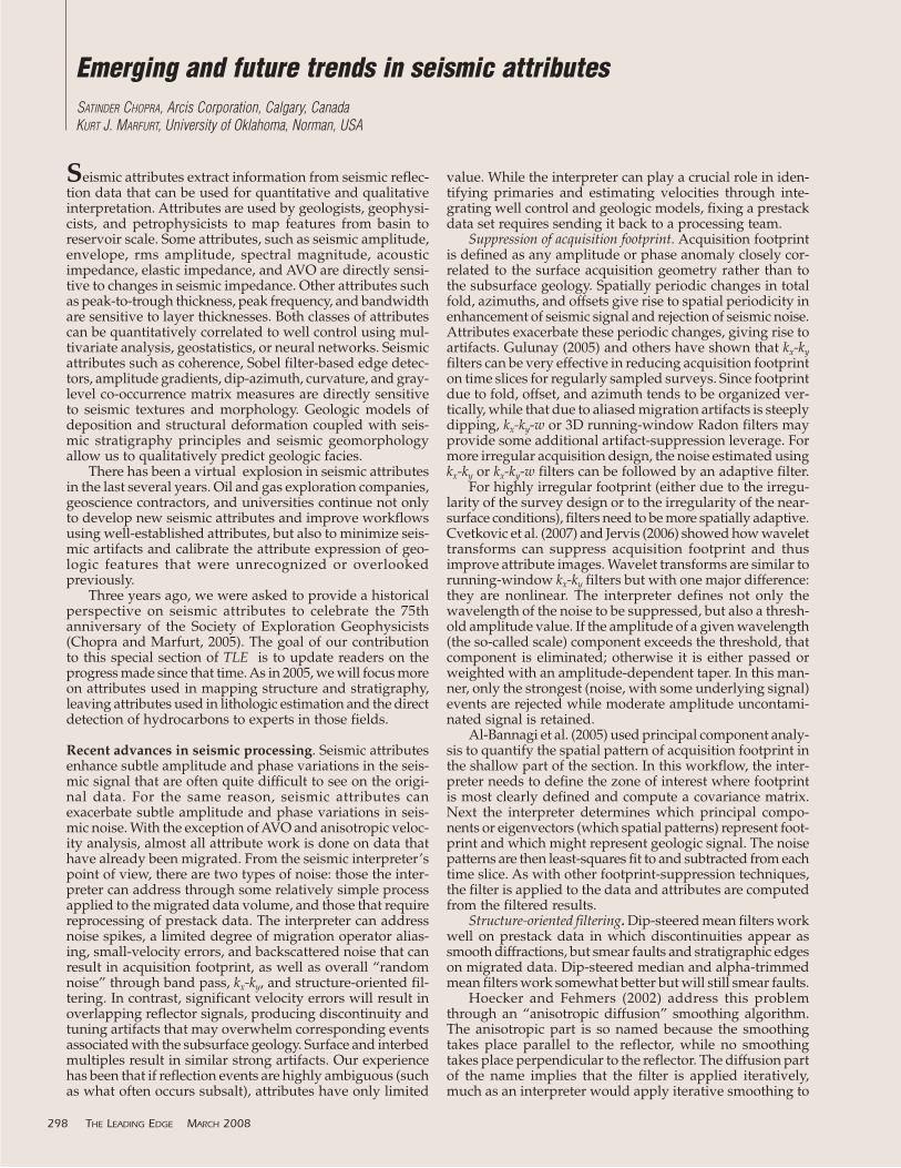
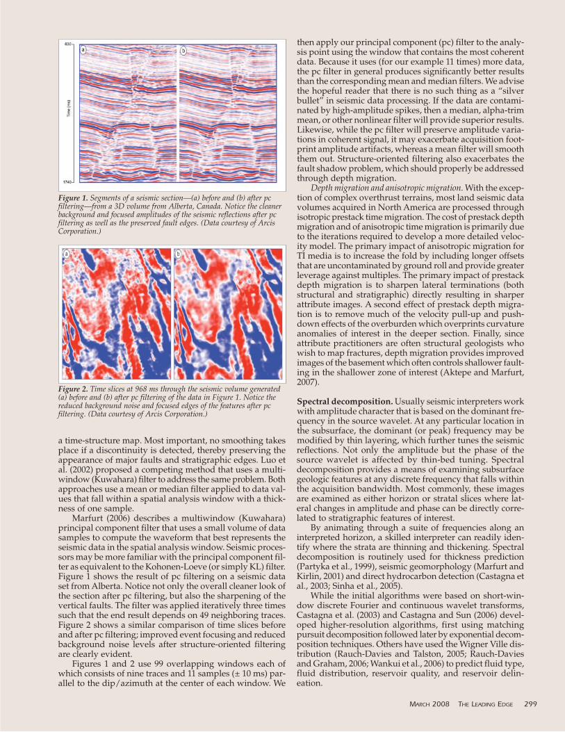
Marfurt (2006) describes a multiwindow (Kuwahara)principal component filter that uses a small volume of datasamples to compute the waveform that best represents theseismic data in the spatial analysis window. Seismic proces-sors may be more familiar with the principal component fil-ter as equivalent to the Kohonen-Loeve (or simply KL) filter.Figure 1 shows the result of pc filtering on a seismic dataset from Alberta. Notice not only the overall cleaner look ofthe section after pc filtering, but also the sharpening of thevertical faults. The filter was applied iteratively three timessuch that the end result depends on 49 neighboring traces.Figure 2 shows a similar comparison of time slices beforeand after pc filtering; improved event focusing and reducedbackground noise levels after structure-oriented filteringare clearly evident.

Figures 1 and 2 use 99 overlapping windows each ofwhich consists of nine traces and 11 samples (± 10 ms) par-allel to the dip/azimuth at the center of each window. We

then apply our principal component (pc) filter to the analy-sis point using the window that contains the most coherentdata. Because it uses (for our example 11 times) more data,the pc filter in general produces significantly better resultsthan the corresponding mean and median filters. We advisethe hopeful reader that there is no such thing as a “silverbullet” in seismic data processing. If the data are contami-nated by high-amplitude spikes, then a median, alpha-trimmean, or other nonlinear filter will provide superior results.Likewise, while the pc filter will preserve amplitude varia-tions in coherent signal, it may exacerbate acquisition foot-print amplitude artifacts, whereas a mean filter will smooththem out. Structure-oriented filtering also exacerbates thefault shadow problem, which should properly be addressedthrough depth migration.

Depth migration and anisotropic migration. With the excep-tion of complex overthrust terrains, most land seismic datavolumes acquired in North America are processed throughisotropic prestack time migration. The cost of prestack depthmigration and of anisotropic time migration is primarily dueto the iterations required to develop a more detailed veloc-ity model. The primary impact of anisotropic migration forTI media is to increase the fold by including longer offsetsthat are uncontaminated by ground roll and provide greaterleverage against multiples. The primary impact of prestackdepth migration is to sharpen lateral terminations (bothstructural and stratigraphic) directly resulting in sharperattribute images. A second effect of prestack depth migra-tion is to remove much of the velocity pull-up and push-down effects of the overburden which overprints curvatureanomalies of interest in the deeper section. Finally, sinceattribute practitioners are often structural geologists whowish to map fractures, depth migration provides improvedimages of the basement which often controls shallower fault-ing in the shallower zone of interest (Aktepe and Marfurt,2007).

Spectral decomposition. Usually seismic interpreters workwith amplitude character that is based on the dominant fre-quency in the source wavelet. At any particular location inthe subsurface, the dominant (or peak) frequency may bemodified by thin layering, which further tunes the seismicreflections. Not only the amplitude but the phase of thesource wavelet is affected by thin-bed tuning. Spectraldecomposition provides a means of examining subsurfacegeologic features at any discrete frequency that falls withinthe acquisition bandwidth. Most commonly, these imagesare examined as either horizon or stratal slices where lat-eral changes in amplitude and phase can be directly corre-lated to stratigraphic features of interest.

By animating through a suite of frequencies along aninterpreted horizon, a skilled interpreter can readily iden-tify where the strata are thinning and thickening. Spectraldecomposition is routinely used for thickness prediction(Partyka et al., 1999), seismic geomorphology (Marfurt andKirlin, 2001) and direct hydrocarbon detection (Castagna etal., 2003; Sinha et al., 2005).

While the initial algorithms were based on short-win-dow discrete Fourier and continuous wavelet transforms,Castagna et al. (2003) and Castagna and Sun (2006) devel-oped higher-resolution algorithms, first using matching pursuit decomposition followed later by exponential decom-position techniques. Others have used the Wigner Ville dis-tribution (Rauch-Davies and Talston, 2005; Rauch-Daviesand Graham, 2006; Wankui et al., 2006) to predict fluid type,fluid distribution, reservoir quality, and reservoir delin-eation.

MARCH 2008 THE LEADING EDGE 299

Figure 1. Segments of a seismic section—(a) before and (b) after pcfiltering—from a 3D volume from Alberta, Canada. Notice the cleanerbackground and focused amplitudes of the seismic reflections after pcfiltering as well as the preserved fault edges. (Data courtesy of ArcisCorporation.)

Figure 2. Time slices at 968 ms through the seismic volume generated(a) before and (b) after pc filtering of the data in Figure 1. Notice thereduced background noise and focused edges of the features after pcfiltering. (Data courtesy of Arcis Corporation.)

Spectral decomposition has been applied not only totime domain, but to depth domain data as well. Montoyaet al. (2005) demonstrate the application of spectral decom-position in the depth domain to an area in the Gulf ofMexico, which helped understand the distribution and clas-sification of deepwater geologic elements.

Discontinuities in spectra to map unconformities. In their firstpaper on instantaneous attributes, Taner et al. (1979) rec-ognized that waveform interference gives rise to disconti-nuities in instantaneous phase. These discontinuities in turngive rise to singularities in the time derivative of instanta-neous phase, or instantaneous frequency. At first they suppressed these singularities by computing an envelope-weighted average frequency, which emphasized changes inphase near the envelope peaks where waveform interfer-ence is minimal. Later, they enhanced these discontinuitiesby subtracting the envelope-weighted average frequencyfrom the instantaneous frequency, giving rise to what theycalled a thin-bed indicator.

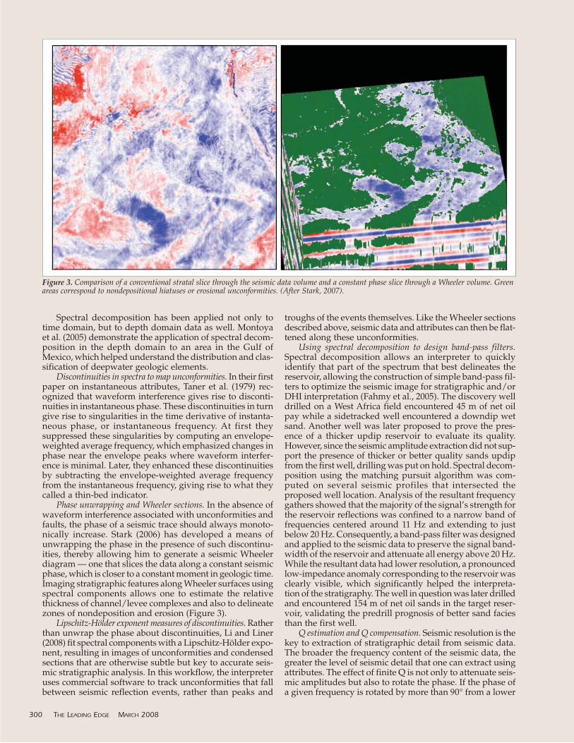
Phase unwrapping and Wheeler sections. In the absence ofwaveform interference associated with unconformities andfaults, the phase of a seismic trace should always monoto-nically increase. Stark (2006) has developed a means ofunwrapping the phase in the presence of such discontinu-ities, thereby allowing him to generate a seismic Wheelerdiagram — one that slices the data along a constant seismicphase, which is closer to a constant moment in geologic time.Imaging stratigraphic features along Wheeler surfaces usingspectral components allows one to estimate the relativethickness of channel/levee complexes and also to delineatezones of nondeposition and erosion (Figure 3).

Lipschitz-Hölder exponent measures of discontinuities. Ratherthan unwrap the phase about discontinuities, Li and Liner(2008) fit spectral components with a Lipschitz-Hölder expo-nent, resulting in images of unconformities and condensedsections that are otherwise subtle but key to accurate seis-mic stratigraphic analysis. In this workflow, the interpreteruses commercial software to track unconformities that fallbetween seismic reflection events, rather than peaks and

troughs of the events themselves. Like the Wheeler sectionsdescribed above, seismic data and attributes can then be flat-tened along these unconformities.

Using spectral decomposition to design band-pass filters.Spectral decomposition allows an interpreter to quicklyidentify that part of the spectrum that best delineates thereservoir, allowing the construction of simple band-pass fil-ters to optimize the seismic image for stratigraphic and/orDHI interpretation (Fahmy et al., 2005). The discovery welldrilled on a West Africa field encountered 45 m of net oilpay while a sidetracked well encountered a downdip wetsand. Another well was later proposed to prove the pres-ence of a thicker updip reservoir to evaluate its quality.However, since the seismic amplitude extraction did not sup-port the presence of thicker or better quality sands updipfrom the first well, drilling was put on hold. Spectral decom-position using the matching pursuit algorithm was com-puted on several seismic profiles that intersected theproposed well location. Analysis of the resultant frequencygathers showed that the majority of the signal’s strength forthe reservoir reflections was confined to a narrow band offrequencies centered around 11 Hz and extending to justbelow 20 Hz. Consequently, a band-pass filter was designedand applied to the seismic data to preserve the signal band-width of the reservoir and attenuate all energy above 20 Hz.While the resultant data had lower resolution, a pronouncedlow-impedance anomaly corresponding to the reservoir wasclearly visible, which significantly helped the interpreta-tion of the stratigraphy. The well in question was later drilledand encountered 154 m of net oil sands in the target reser-voir, validating the predrill prognosis of better sand faciesthan the first well.

Q estimation and Q compensation. Seismic resolution is thekey to extraction of stratigraphic detail from seismic data.The broader the frequency content of the seismic data, thegreater the level of seismic detail that one can extract usingattributes. The effect of finite Q is not only to attenuate seis-mic amplitudes but also to rotate the phase. If the phase ofa given frequency is rotated by more than 90° from a lower


Figure 3. Comparison of a conventional stratal slice through the seismic data volume and a constant phase slice through a Wheeler volume. Greenareas correspond to nondepositional hiatuses or erosional unconformities. (After Stark, 2007).

reference frequency, no amount of amplitude compensationwill allow it to constructively contribute to generating a broad-band reflection. In the processing shop, poststack or prestackspectral whitening (or Q-compensation for seismic ampli-tude) is often applied to enhance the spectral bandwidth ofthe data prior to interpretation. Recent advances in comput-

ing spectral compon-ents havelead to improved estimation ofseismic attenuation (1/Q) usingthe well-established spectral ratiotechnique. While Q-compensa-tion is routinely applied to seis-mic amplitudes, Q-compensationapplied to seismic phases is amore recent development (Wang,2006). Based on the same model-based physics as earlier develop-ments by Taner and Treitel (2003)and Chopra et al. (2003) thatexploited the additional infor-mation provided by either welllogs or VSPs, this more recentdevelopment is based on the seis-mic data alone.

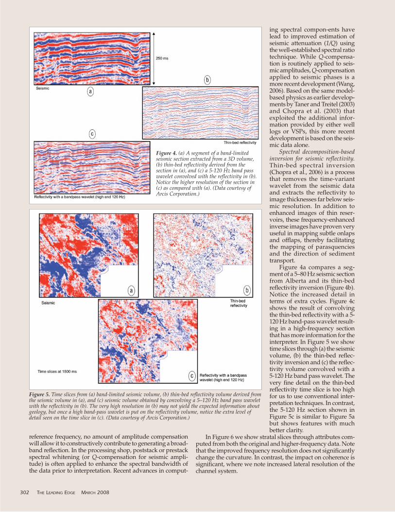
Spectral decomposition-basedinversion for seismic reflectivity.Thin-bed spectral inversion(Chopra et al., 2006) is a processthat removes the time-variantwavelet from the seismic dataand extracts the reflectivity toimage thicknesses far below seis-mic resolution. In addition toenhanced images of thin reser-voirs, these frequency-enhancedinverse images have proven veryuseful in mapping subtle onlapsand offlaps, thereby facilitatingthe mapping of parasquenciesand the direction of sedimenttransport.

Figure 4a compares a seg-ment of a 5–80 Hz seismic sectionfrom Alberta and its thin-bedreflectivity inversion (Figure 4b).Notice the increased detail interms of extra cycles. Figure 4cshows the result of convolvingthe thin-bed reflectivity with a 5-120 Hz band-pass wavelet result-ing in a high-frequency sectionthat has more information for theinterpreter. In Figure 5 we showtime slices through (a) the seismicvolume, (b) the thin-bed reflec-tivity inversion and (c) the reflec-tivity volume convolved with a5-120 Hz band pass wavelet. Thevery fine detail on the thin-bedreflectivity time slice is too highfor us to use conventional inter-pretation techniques. In contrast,the 5-120 Hz section shown inFigure 5c is similar to Figure 5abut shows features with muchbetter clarity.

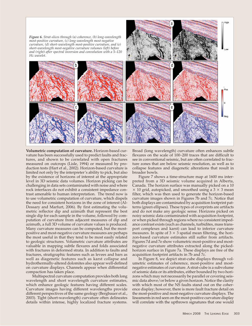
In Figure 6 we show stratal slices through attributes com-puted from both the original and higher-frequency data. Notethat the improved frequency resolution does not significantlychange the curvature. In contrast, the impact on coherence issignificant, where we note increased lateral resolution of thechannel system.


Figure 4. (a) A segment of a band-limitedseismic section extracted from a 3D volume,(b) thin-bed reflectivity derived from thesection in (a), and (c) a 5-120 Hz band passwavelet convolved with the reflectivity in (b).Notice the higher resolution of the section in(c) as compared with (a). (Data courtesy ofArcis Corporation.)

Figure 5. Time slices from (a) band-limited seismic volume, (b) thin-bed reflectivity volume derived fromthe seismic volume in (a), and (c) seismic volume obtained by convolving a 5–120 Hz band pass waveletwith the reflectivity in (b). The very high resolution in (b) may not yield the expected information aboutgeology, but once a high band-pass wavelet is put on the reflectivity volume, notice the extra level ofdetail seen on the time slice in (c). (Data courtesy of Arcis Corporation.)

Volumetric computation of curvature. Horizon-based cur-vature has been successfully used to predict faults and frac-tures, and shown to be correlated with open fracturesmeasured on outcrops (Lisle, 1994) or measured by pro-duction tests (Hart et al., 2002). Horizon-based curvature islimited not only by the interpreter’s ability to pick, but alsoby the existence of horizons of interest at the appropriatelevel in 3D seismic data volumes. Horizon picking can bechallenging in data sets contaminated with noise and whererock interfaces do not exhibit a consistent impedance con-trast amenable to human interpretation. The trend now isto use volumetric computation of curvature, which dispelsthe need for consistent horizons in the zone of interest (Al-Dossary and Marfurt, 2006). By first estimating the volu-metric reflector dip and azimuth that represent the bestsingle dip for each sample in the volume, followed by com-putation of curvature from adjacent measures of dip andazimuth, a full 3D volume of curvature values is produced.Many curvature measures can be computed, but the most-positive and most-negative curvature measures are perhapsthe most useful in that they tend to be most easily relatedto geologic structures. Volumetric curvature attributes arevaluable in mapping subtle flexures and folds associatedwith fractures in deformed strata. In addition to faults andfractures, stratigraphic features such as levees and bars aswell as diagenetic features such as karst collapse andhydrothermally-altered dolomites also appear well-definedon curvature displays. Channels appear when differentialcompaction has taken place.

Multispectral curvature computation provides both longwavelength and short wavelength curvature estimates,which enhance geologic features having different scales.Curvature images having different wavelengths providedifferent perspectives of the same geology (Bergbauer et al.,2003). Tight (short-wavelength) curvature often delineatesdetails within intense, highly localized fracture systems.

Broad (long wavelength) curvature often enhances subtleflexures on the scale of 100–200 traces that are difficult tosee in conventional seismic, but are often correlated to frac-ture zones that are below seismic resolution, as well as tocollapse features and diagenetic alterations that result inbroader bowls.

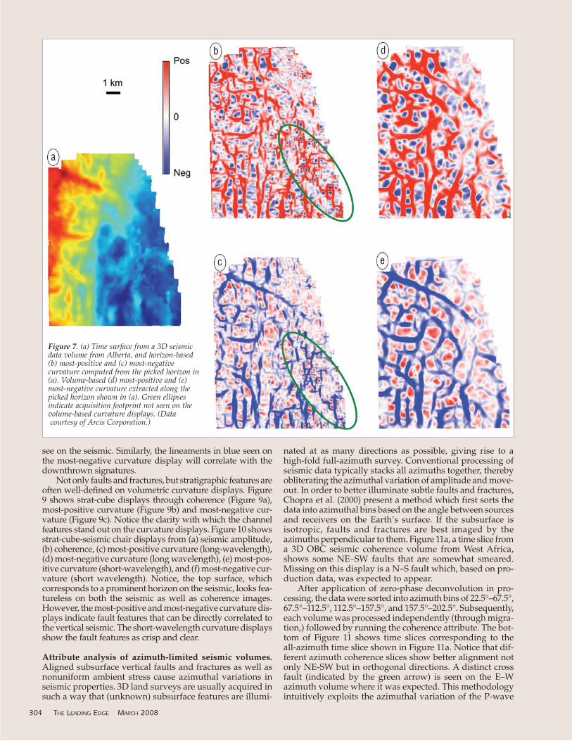
Figure 7 shows a time-structure map at 1600 ms inter-preted from a 3D seismic volume acquired in Alberta,Canada. The horizon surface was manually picked on a 10� 10 grid, autopicked, and smoothed using a 3 � 3 meanfilter, which was then used to generate the horizon-basedcurvature images shown in Figures 7b and 7c. Notice thatboth displays are contaminated by acquisition footprint pat-terns (green ellipses). These types of overprints are artifactsand do not make any geologic sense. Horizons picked onnoisy seismic data contaminated with acquisition footprint,or when picked through regions where no consistent imped-ance contrast exists (such as channels, turbidites, mass trans-port complexes and karst) can lead to inferior curvaturemeasures. In spite of 3 � 3 spatial mean filtering, the hori-zon-based curvature estimates still suffer from artifacts.Figures 7d and 7e show volumetric most-positive and most-negative curvature attributes extracted along the picked-horizon surface in Figure 7a. These displays are free of theacquisition footprint artifacts in 7b and 7c.

In Figure 8, we depict strat-cube displays through vol-umetric estimates of coherence, most-positive and most-negative estimates of curvature. A strat-cube is a subvolumeof seismic data or its attributes, either bounded by two hori-zons which may not necessarily be parallel or covering seis-mic data above/or below a given horizon. Notice the claritywith which most of the NS faults stand out on the coher-ence display; however, there is more fault fracture detail onthe most-positive and most-negative curvature displays. Thelineaments in red seen on the most-positive curvature displaywill correlate with the upthrown signatures that one would


Figure 6. Strat-slices through (a) coherence, (b) long-wavelengthmost-positive curvature, (c) long-wavelength most-negative curvature, (d) short-wavelength most-positive curvature, and (e)short-wavelength most-negative curvature volumes (left) beforeand (right) after spectral inversion and convolution with a 5–120Hz wavelet.

see on the seismic. Similarly, the lineaments in blue seen onthe most-negative curvature display will correlate with thedownthrown signatures.

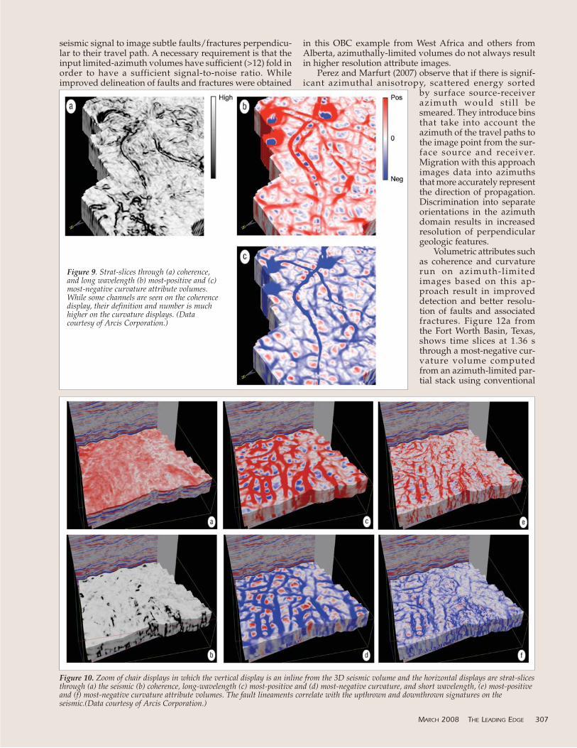
Not only faults and fractures, but stratigraphic features areoften well-defined on volumetric curvature displays. Figure9 shows strat-cube displays through coherence (Figure 9a),most-positive curvature (Figure 9b) and most-negative cur-vature (Figure 9c). Notice the clarity with which the channelfeatures stand out on the curvature displays. Figure 10 showsstrat-cube-seismic chair displays from (a) seismic amplitude,(b) coherence, (c) most-positive curvature (long-wavelength),(d) most-negative curvature (long wavelength), (e) most-pos-itive curvature (short-wavelength), and (f) most-negative cur-vature (short wavelength). Notice, the top surface, whichcorresponds to a prominent horizon on the seismic, looks fea-tureless on both the seismic as well as coherence images.However, the most-positive and most-negative curvature dis-plays indicate fault features that can be directly correlated tothe vertical seismic. The short-wavelength curvature displaysshow the fault features as crisp and clear.

Attribute analysis of azimuth-limited seismic volumes.Aligned subsurface vertical faults and fractures as well asnonuniform ambient stress cause azimuthal variations inseismic properties. 3D land surveys are usually acquired insuch a way that (unknown) subsurface features are illumi-

nated at as many directions as possible, giving rise to ahigh-fold full-azimuth survey. Conventional processing ofseismic data typically stacks all azimuths together, therebyobliterating the azimuthal variation of amplitude and move-out. In order to better illuminate subtle faults and fractures,Chopra et al. (2000) present a method which first sorts thedata into azimuthal bins based on the angle between sourcesand receivers on the Earth’s surface. If the subsurface isisotropic, faults and fractures are best imaged by theazimuths perpendicular to them. Figure 11a, a time slice froma 3D OBC seismic coherence volume from West Africa,shows some NE–SW faults that are somewhat smeared.Missing on this display is a N–S fault which, based on pro-duction data, was expected to appear.

After application of zero-phase deconvolution in pro-cessing, the data were sorted into azimuth bins of 22.5°–67.5°,67.5°–112.5°, 112.5°–157.5°, and 157.5°–202.5°. Subsequently,each volume was processed independently (through migra-tion,) followed by running the coherence attribute. The bot-tom of Figure 11 shows time slices corresponding to theall-azimuth time slice shown in Figure 11a. Notice that dif-ferent azimuth coherence slices show better alignment notonly NE-SW but in orthogonal directions. A distinct crossfault (indicated by the green arrow) is seen on the E–Wazimuth volume where it was expected. This methodologyintuitively exploits the azimuthal variation of the P-wave


Figure 7. (a) Time surface from a 3D seismicdata volume from Alberta, and horizon-based(b) most-positive and (c) most-negative curvature computed from the picked horizon in(a). Volume-based (d) most-positive and (e)most-negative curvature extracted along thepicked horizon shown in (a). Green ellipsesindicate acquisition footprint not seen on thevolume-based curvature displays. (Datacourtesy of Arcis Corporation.)


Figure 8. Strat cubes through (a) coherence, and long-wavelength (b) most-positive, and (c) most-negative attribute volumes. (d) Color stack of allthree attributes. While some N–S faults are seen on the coherence display, the level of detail is much higher on the curvature displays. (Datacourtesy of Arcis Corporation.)

seismic signal to image subtle faults/fractures perpendicu-lar to their travel path. A necessary requirement is that theinput limited-azimuth volumes have sufficient (>12) fold inorder to have a sufficient signal-to-noise ratio. Whileimproved delineation of faults and fractures were obtained

in this OBC example from West Africa and others fromAlberta, azimuthally-limited volumes do not always resultin higher resolution attribute images.

Perez and Marfurt (2007) observe that if there is signif-icant azimuthal anisotropy, scattered energy sorted

by surface source-receiverazimuth would still besmeared. They introduce binsthat take into account theazimuth of the travel paths tothe image point from the sur-face source and receiver.Migration with this approachimages data into azimuthsthat more accurately representthe direction of propagation.Discrimination into separateorientations in the azimuthdomain results in increasedresolution of perpendiculargeologic features.

Volumetric attributes suchas coherence and curvaturerun on azimuth-limitedimages based on this ap-proach result in improveddetection and better resolu-tion of faults and associated fractures. Figure 12a from the Fort Worth Basin, Texas,shows time slices at 1.36 sthrough a most-negative cur-vature volume computedfrom an azimuth-limited par-tial stack using conventional


Figure 9. Strat-slices through (a) coherence,and long wavelength (b) most-positive and (c)most-negative curvature attribute volumes.While some channels are seen on the coherencedisplay, their definition and number is muchhigher on the curvature displays. (Data courtesy of Arcis Corporation.)

Figure 10. Zoom of chair displays in which the vertical display is an inline from the 3D seismic volume and the horizontal displays are strat-slicesthrough (a) the seismic (b) coherence, long-wavelength (c) most-positive and (d) most-negative curvature, and short wavelength, (e) most-positiveand (f) most-negative curvature attribute volumes. The fault lineaments correlate with the upthrown and downthrown signatures on the seismic.(Data courtesy of Arcis Corporation.)

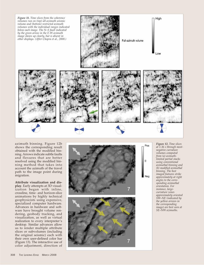
azimuth binning. Figure 12bshows the corresponding resultobtained with the modified bin-ning. Arrows indicate subtle faultsand flexures that are betterresolved using the modified bin-ning method that takes intoaccount the azimuth of the travelpath to the image point duringmigration.

Attribute visualization and dis-play. Early attempts at 3D visual-ization began with inline,crossline, time- and horizon-sliceanimations by highly technicalgeophysicists using expensive,specialized computer hardware.Advances in hardware and soft-ware have brought volume ren-dering, geobody tracking, andvisualization, as well as virtualrealization to every interpreter’sdesktop. Similar advances allowus to render multiple attributeslices or subvolumes (includingthe original seismic) each withtheir own user-defined color bar(Figure 13). The interactive use ofcolor adjustment, direction of


Figure 12. Time slicesat 1.36 s through most-negative curvaturevolumes computedfrom (a) azimuth-limited partial stacksusing conventionalazimuthal binning and(b) modified azimuthalbinning. The bestimaged features strikeapproximately at rightangles to the corre-sponding azimuthalorientation. Forinstance, large-curvature zonesapproximately orientedSW–NE (indicated bythe yellow arrows inthe correspondingimage) are best seen atSE–NW azimuths.

Figure 11. Time slices from the coherencevolumes run on (top) all-azimuth seismicvolume and (bottom) restricted azimuthvolumes with the individual ranges indicatedbelow each image. The N–S fault indicatedby the green arrow in the E-W azimuthimage shows up clearly, but is absent inother displays. (After Chopra et al., 2000.)

lighting, and opacity allows the interpreter to highlight sub-tle stratigraphic detail that otherwise could be missed.

All commercial workstations have the ability to plot asingle seismic or attribute volume against 256 discrete col-ors displayed as single gradational, dual gradational, or

cyclical 1D color bars. Mostworkstations allow the inter-preter to modulate this color barwith a 1D opacity control,thereby enhancing 3D volumet-ric views of voxels whose valuesfall with a user-defined range.Modern workstations also allowthe visualization of multipleattribute vertical, time, horizon,or stratal slices, as well as sub-volumes, in the same image,each with its own unique colorbar. We demonstrate this capa-bility in Figure 13, where wecorender stratal slices throughcoherence, most-positive curva-ture, and most-negative curva-ture with several seismicsubvolumes. Such co-renderingcapabilities are key to visuallycalibrating geomorphologicalfeatures and structural linea-ments seen on stratal and hori-zon slices with the seismicamplitude signature seen onvertical slices to ascertainwhether the features are indeedgeologic, or a seismic acquisi-tion or processing artifact. Theinterpreter can interactivelyrotate the volume display in anydirection to better understandthe data disposition.

Several workstation imple-mentations allow the interpreterto plot different attributesagainst red, green, and blue pri-mary colors. Guo et al. (2008)find that this color model worksbest when attributes are of sim-ilar type, such as near-, mid-,and far-offset seismic ampli-tudes. Giroldi and Alegria (2005)use the RGB color model to plotspectral components of 20, 25,and 30 Hz to generate the com-posite image in Figure 14. A sys-tem of channels, clearly seen onthe multiattribute spectraldecomposition image, are diffi-cult to see on the rms amplitudeimage even though both extrac-tions were made using the sametime interval and calculatedwith an equivalent window size.

Guo et al. show how the hue-lightness-saturation (HLS) colormodel can be constructed to dis-play a second or third attribute.The HLS color bar is displayedalternatively as a three-axis dual

pyramid, sphere, or cylinder developed by Munsell earlyin the twentieth century and shown in Figure 15. WhileRijks and Jauffred (1991) used a 2D hue-lightness color barover 15 years ago, such capabilities were not available incommercial software until the introduction of “attribute cal-


Figure 13. Covisualization of seismic subvolumes and strat cubes from (a) coherence (b) most-positiveand (c) most-negative curvature volumes. Several channels are seen on the coherence strat cube, but amore complete system is seen on the most-negative curvature (which delineates the channel axes, orthalwegs) and most-positive curvature (which delineates the channel flanks). (Data courtesy of ArcisCorporation.)

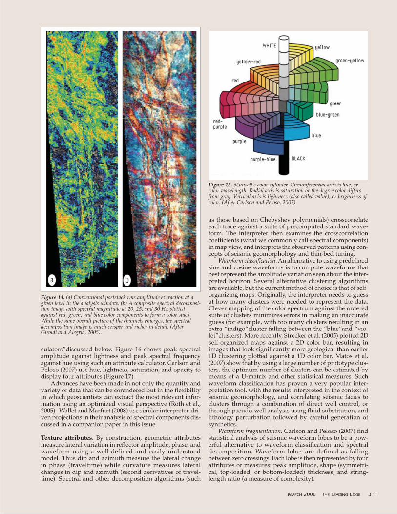
culators”discussed below. Figure 16 shows peak spectralamplitude against lightness and peak spectral frequencyagainst hue using such an attribute calculator. Carlson andPeloso (2007) use hue, lightness, saturation, and opacity todisplay four attributes (Figure 17).

Advances have been made in not only the quantity andvariety of data that can be corendered but in the flexibilityin which geoscientists can extract the most relevant infor-mation using an optimized visual perspective (Roth et al.,2005). Wallet and Marfurt (2008) use similar interpreter-dri-ven projections in their analysis of spectral components dis-cussed in a companion paper in this issue.

Texture attributes. By construction, geometric attributesmeasure lateral variation in reflector amplitude, phase, andwaveform using a well-defined and easily understoodmodel. Thus dip and azimuth measure the lateral changein phase (traveltime) while curvature measures lateralchanges in dip and azimuth (second derivatives of travel-time). Spectral and other decomposition algorithms (such

as those based on Chebyshev polynomials) crosscorrelateeach trace against a suite of precomputed standard wave-form. The interpreter then examines the crosscorrelationcoefficients (what we commonly call spectral components)in map view, and interprets the observed patterns using con-cepts of seismic geomorphology and thin-bed tuning.

Waveform classification. An alternative to using predefinedsine and cosine waveforms is to compute waveforms thatbest represent the amplitude variation seen about the inter-preted horizon. Several alternative clustering algorithmsare available, but the current method of choice is that of self-organizing maps. Originally, the interpreter needs to guessat how many clusters were needed to represent the data.Clever mapping of the color spectrum against the orderedsuite of clusters minimizes errors in making an inaccurateguess (for example, with too many clusters resulting in anextra “indigo”cluster falling between the “blue”and “vio-let”clusters). More recently, Strecker et al. (2005) plotted 2Dself-organized maps against a 2D color bar, resulting inimages that look significantly more geological than earlier1D clustering plotted against a 1D color bar. Matos et al.(2007) show that by using a large number of prototype clus-ters, the optimum number of clusters can be estimated bymeans of a U-matrix and other statistical measures. Suchwaveform classification has proven a very popular inter-pretation tool, with the results interpreted in the context ofseismic geomorphology, and correlating seismic facies toclusters through a combination of direct well control, orthrough pseudo-well analysis using fluid substitution, andlithology perturbation followed by careful generation ofsynthetics.

Waveform fragmentation. Carlson and Peloso (2007) findstatistical analysis of seismic waveform lobes to be a pow-erful alternative to waveform classification and spectraldecomposition. Waveform lobes are defined as fallingbetween zero crossings. Each lobe is then represented by fourattributes or measures: peak amplitude, shape (symmetri-cal, top-loaded, or bottom-loaded) thickness, and string-length ratio (a measure of complexity).


Figure 14. (a) Conventional poststack rms amplitude extraction at agiven level in the analysis window. (b) A composite spectral decomposi-tion image with spectral magnitude at 20, 25, and 30 Hz plottedagainst red, green, and blue color components to form a color stack.While the same overall picture of the channels emerges, the spectraldecomposition image is much crisper and richer in detail. (AfterGiroldi and Alegria, 2005).

Figure 15. Munsell’s color cylinder. Circumferential axis is hue, orcolor wavelength. Radial axis is saturation or the degree color differsfrom gray. Vertical axis is lightness (also called value), or brightness ofcolor. (After Carlson and Peloso, 2007).

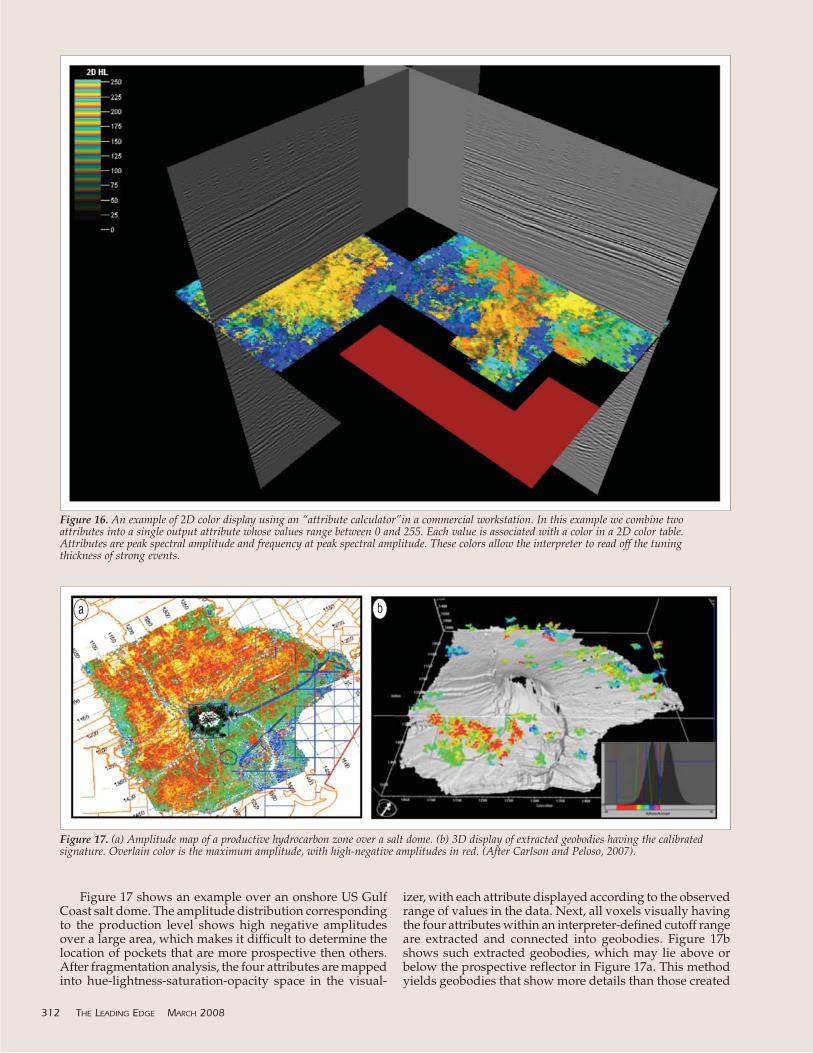
Figure 17 shows an example over an onshore US GulfCoast salt dome. The amplitude distribution correspondingto the production level shows high negative amplitudesover a large area, which makes it difficult to determine thelocation of pockets that are more prospective then others.After fragmentation analysis, the four attributes are mappedinto hue-lightness-saturation-opacity space in the visual-

izer, with each attribute displayed according to the observedrange of values in the data. Next, all voxels visually havingthe four attributes within an interpreter-defined cutoff rangeare extracted and connected into geobodies. Figure 17bshows such extracted geobodies, which may lie above orbelow the prospective reflector in Figure 17a. This methodyields geobodies that show more details than those created


Figure 16. An example of 2D color display using an “attribute calculator”in a commercial workstation. In this example we combine two attributes into a single output attribute whose values range between 0 and 255. Each value is associated with a color in a 2D color table.Attributes are peak spectral amplitude and frequency at peak spectral amplitude. These colors allow the interpreter to read off the tuning thickness of strong events.

Figure 17. (a) Amplitude map of a productive hydrocarbon zone over a salt dome. (b) 3D display of extracted geobodies having the calibratedsignature. Overlain color is the maximum amplitude, with high-negative amplitudes in red. (After Carlson and Peloso, 2007).

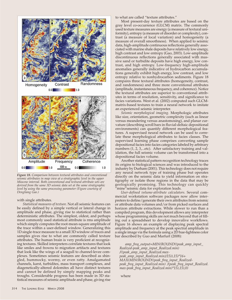
with single attributes.Statistical measures of texture. Not all seismic features can

be easily defined by a simple vertical or lateral change inamplitude and phase, giving rise to statistical rather thandeterministic attributes. The simplest, oldest, and perhapsmost commonly used statistical attribute is rms amplitudewhich simply computes the root-mean-square amplitude ofthe trace within a user-defined window. Generalizing this1D single-trace measure to a small 3D window of traces andsamples gives rise to what are commonly called textureattributes. The human brain is very proficient at recogniz-ing textures. Skilled interpreters correlate textures that looklike smiles and frowns to migration artifacts and texturesthat look like the wings of a seagull to channel-levee com-plexes. Sometimes seismic features are described as shin-gled, hummocky, wormy, or even ratty. Amalgamatedchannels, karst, turbidites, mass transport complexes, anddiagenetically-altered dolomites all have distinct texturesand cannot be defined by simply mapping peaks andtroughs. Considerable progress has been made in 3D sta-tistical measures of seismic amplitude and phase, giving rise

to what are called “texture attributes.”Most present-day texture attributes are based on the

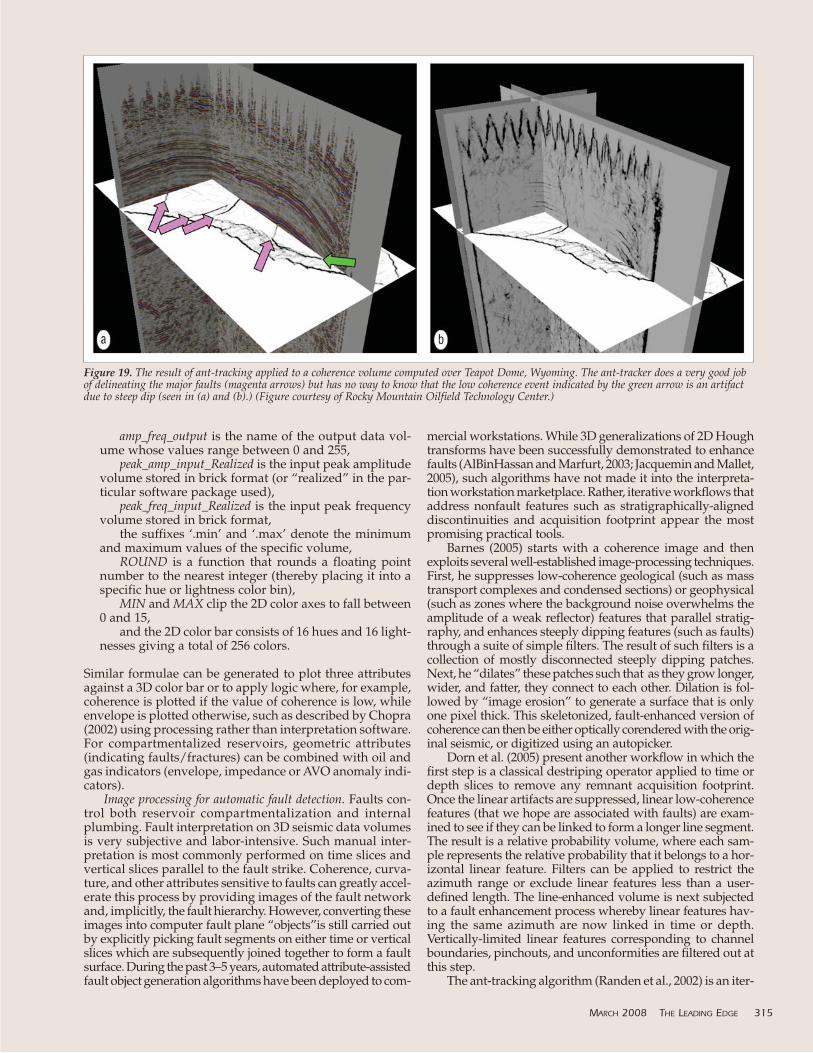
gray level co-occurrence (GLCM) matrix. The commonlyused texture measures are energy (a measure of textural uni-formity), entropy (a measure of disorder or complexity), con-trast (a measure of local variation) and homogeneity (ameasure of overall smoothness). When applied to seismicdata, high-amplitude continuous reflections generally asso-ciated with marine shale deposits have relatively low energy,high contrast and low entropy (Gao, 2003). Low-amplitudediscontinuous reflections generally associated with mas-sive sand or turbidite deposits have high energy, low con-trast, and high entropy. Low-frequency high-amplitudeanomalies generally indicative of hydrocarbon accumula-tions generally exhibit high energy, low contrast, and lowentropy relative to nonhydrocarbon sediments. Figure 18compares three textural attributes (homogeneity, contrast,and randomness) and three more conventional attributes(amplitude, instantaneous frequency, and coherence). Noticethe textural attributes are superior to conventional attrib-utes in terms of resolution, sensitivity, and significance tofacies variations. West et al. (2002) computed such GLCM-matrix-based textures to train a neural network to imitatean experienced seismic interpreter.

Seismic morphological imaging. Morphologic attributeslike size, orientation, geometric complexity (such as linearversus meandering versus anastomosing), and planar cur-vature (describing scroll bars in fluvial-deltaic depositionalenvironments) can quantify different morphological fea-tures. A supervised neural network can be used to corre-late these morphological attributes to facies classes. Thesupervised learning phase comprises converting sampledepositional facies into facies categories labeled by arbitrarynumbers (1, 2, 3,...etc). After satisfactory training and val-idation, the full seismic volume can be transformed into adepositional facies volume.

Another statistical pattern recognition technology tracesits origins to biological sciences and was introduced to theindustry by Durham (2001). This technology does not requireany neural network type of training phase but operatesdirectly on the seismic data to yield information on stra-tigraphy or isolate those regions in the data that may be geologically promising. This technology can quickly“mine”seismic data for exploration leads.

User-defined volume-attribute calculators. Several com-mercial workstation software packages now allow inter-preters to define/generate their own attributes from seismicor attribute data volumes and/or from picked surfaces andhorizon attribute extractions. While slower to run than acompiled program, this development allows any interpreterwhose programming skills are not much beyond that of fill-ing out a spreadsheet to develop innovative workflows.Figure 16 shows an example of displaying peak spectralamplitude and frequency at the peak spectral amplitude ina single image via the formula using a 2D hue-lightness colorbar described by Guo and Marfurt (2008):

amp_freq_output=MIN(ROUND((peak_amp_input_Realized-peak_amp_input_Realized.min)/((peak_amp_input_Realized.max-peak_amp_input_Realized.min)/15)),15)*16+MAX(MIN(ROUND((peak_freq_input_Realized-peak_freq_input_Realized.min) /(peak_freq_input_Realized.max-peak_freq_input_Realized.min)*15),15),0)

where


Figure 18. Comparison between textural attributes and conventionalseismic attributes in map view at a stratigraphic level in the upperMiocene interval. Both conventional and textural attribute sets arederived from the same 3D seismic data set at the same stratigraphiclevel by using the same processing parameter (Figure courtesy ofDengliang Gao.)

amp_freq_output is the name of the output data vol-ume whose values range between 0 and 255,

peak_amp_input_Realized is the input peak amplitudevolume stored in brick format (or “realized” in the par-ticular software package used),

peak_freq_input_Realized is the input peak frequencyvolume stored in brick format,

the suffixes ‘.min’ and ‘.max’ denote the minimumand maximum values of the specific volume,

ROUND is a function that rounds a floating pointnumber to the nearest integer (thereby placing it into aspecific hue or lightness color bin),

MIN and MAX clip the 2D color axes to fall between0 and 15,

and the 2D color bar consists of 16 hues and 16 light-nesses giving a total of 256 colors.

Similar formulae can be generated to plot three attributesagainst a 3D color bar or to apply logic where, for example,coherence is plotted if the value of coherence is low, whileenvelope is plotted otherwise, such as described by Chopra(2002) using processing rather than interpretation software.For compartmentalized reservoirs, geometric attributes(indicating faults/fractures) can be combined with oil andgas indicators (envelope, impedance or AVO anomaly indi-cators).

Image processing for automatic fault detection. Faults con-trol both reservoir compartmentalization and internalplumbing. Fault interpretation on 3D seismic data volumesis very subjective and labor-intensive. Such manual inter-pretation is most commonly performed on time slices andvertical slices parallel to the fault strike. Coherence, curva-ture, and other attributes sensitive to faults can greatly accel-erate this process by providing images of the fault networkand, implicitly, the fault hierarchy. However, converting theseimages into computer fault plane “objects”is still carried outby explicitly picking fault segments on either time or verticalslices which are subsequently joined together to form a faultsurface. During the past 3–5 years, automated attribute-assistedfault object generation algorithms have been deployed to com-

mercial workstations. While 3D generalizations of 2D Houghtransforms have been successfully demonstrated to enhancefaults (AlBinHassan and Marfurt, 2003; Jacquemin and Mallet,2005), such algorithms have not made it into the interpreta-tion workstation marketplace. Rather, iterative workflows thataddress nonfault features such as stratigraphically-aligneddiscontinuities and acquisition footprint appear the mostpromising practical tools.

Barnes (2005) starts with a coherence image and thenexploits several well-established image-processing techniques.First, he suppresses low-coherence geological (such as masstransport complexes and condensed sections) or geophysical(such as zones where the background noise overwhelms theamplitude of a weak reflector) features that parallel stratig-raphy, and enhances steeply dipping features (such as faults)through a suite of simple filters. The result of such filters is acollection of mostly disconnected steeply dipping patches.Next, he “dilates” these patches such that as they grow longer,wider, and fatter, they connect to each other. Dilation is fol-lowed by “image erosion” to generate a surface that is onlyone pixel thick. This skeletonized, fault-enhanced version ofcoherence can then be either optically corendered with the orig-inal seismic, or digitized using an autopicker.

Dorn et al. (2005) present another workflow in which thefirst step is a classical destriping operator applied to time ordepth slices to remove any remnant acquisition footprint.Once the linear artifacts are suppressed, linear low-coherencefeatures (that we hope are associated with faults) are exam-ined to see if they can be linked to form a longer line segment.The result is a relative probability volume, where each sam-ple represents the relative probability that it belongs to a hor-izontal linear feature. Filters can be applied to restrict theazimuth range or exclude linear features less than a user-defined length. The line-enhanced volume is next subjectedto a fault enhancement process whereby linear features hav-ing the same azimuth are now linked in time or depth.Vertically-limited linear features corresponding to channelboundaries, pinchouts, and unconformities are filtered out atthis step.

The ant-tracking algorithm (Randen et al., 2002) is an iter-


Figure 19. The result of ant-tracking applied to a coherence volume computed over Teapot Dome, Wyoming. The ant-tracker does a very good jobof delineating the major faults (magenta arrows) but has no way to know that the low coherence event indicated by the green arrow is an artifactdue to steep dip (seen in (a) and (b).) (Figure courtesy of Rocky Mountain Oilfield Technology Center.)

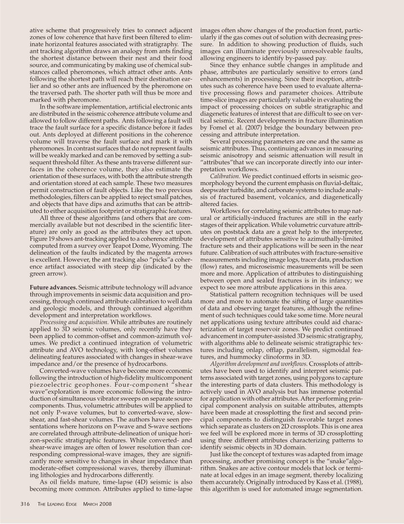
ative scheme that progressively tries to connect adjacentzones of low coherence that have first been filtered to elim-inate horizontal features associated with stratigraphy. Theant tracking algorithm draws an analogy from ants findingthe shortest distance between their nest and their foodsource, and communicating by making use of chemical sub-stances called pheromones, which attract other ants. Antsfollowing the shortest path will reach their destination ear-lier and so other ants are influenced by the pheromone onthe traversed path. The shorter path will thus be more andmarked with pheromone.

In the software implementation, artificial electronic antsare distributed in the seismic coherence attribute volume andallowed to follow different paths. Ants following a fault willtrace the fault surface for a specific distance before it fadesout. Ants deployed at different positions in the coherencevolume will traverse the fault surface and mark it withpheromones. In contrast surfaces that do not represent faultswill be weakly marked and can be removed by setting a sub-sequent threshold filter. As these ants traverse different sur-faces in the coherence volume, they also estimate theorientation of these surfaces, with both the attribute strengthand orientation stored at each sample. These two measurespermit construction of fault objects. Like the two previousmethodologies, filters can be applied to reject small patches,and objects that have dips and azimuths that can be attrib-uted to either acquisition footprint or stratigraphic features.

All three of these algorithms (and others that are com-mercially available but not described in the scientific liter-ature) are only as good as the attributes they act upon.Figure 19 shows ant-tracking applied to a coherence attributecomputed from a survey over Teapot Dome, Wyoming. Thedelineation of the faults indicated by the magenta arrowsis excellent. However, the ant tracking also “picks”a coher-ence artifact associated with steep dip (indicated by thegreen arrow).

Future advances. Seismic attribute technology will advancethrough improvements in seismic data acquisition and pro-cessing, through continued attribute calibration to well dataand geologic models, and through continued algorithmdevelopment and interpretation workflows.

Processing and acquisition. While attributes are routinelyapplied to 3D seismic volumes, only recently have theybeen applied to common-offset and common-azimuth vol-umes. We predict a continued integration of volumetricattribute and AVO technology, with long-offset volumesdelineating features associated with changes in shear-waveimpedance and/or the presence of hydrocarbons.

Converted-wave volumes have become more economicfollowing the introduction of high-fidelity multicomponentpiezoelectric geophones. Four-component “shearwave”exploration is more economic following the intro-duction of simultaneous vibrator sweeps on separate sourcecomponents. Thus, volumetric attributes will be applied tonot only P-wave volumes, but to converted-wave, slow-shear, and fast-shear volumes. The authors have seen pre-sentations where horizons on P-wave and S-wave sectionsare correlated through attribute-delineation of unique hori-zon-specific stratigraphic features. While converted- andshear-wave images are often of lower resolution than cor-responding compressional-wave images, they are signifi-cantly more sensitive to changes in shear impedance thanmoderate-offset compressional waves, thereby illuminat-ing lithologies and hydrocarbons differently.

As oil fields mature, time-lapse (4D) seismic is alsobecoming more common. Attributes applied to time-lapse

images often show changes of the production front, partic-ularly if the gas comes out of solution with decreasing pres-sure. In addition to showing production of fluids, suchimages can illuminate previously unresolveable faults,allowing engineers to identify by-passed pay.

Since they enhance subtle changes in amplitude andphase, attributes are particularly sensitive to errors (andenhancements) in processing. Since their inception, attrib-utes such as coherence have been used to evaluate alterna-tive processing flows and parameter choices. Attributetime-slice images are particularly valuable in evaluating theimpact of processing choices on subtle stratigraphic anddiagenetic features of interest that are difficult to see on ver-tical seismic. Recent developments in fracture illuminationby Fomel et al. (2007) bridge the boundary between pro-cessing and attribute interpretation.

Several processing parameters are one and the same asseismic attributes. Thus, continuing advances in measuringseismic anisotropy and seismic attenuation will result in“attributes”that we can incorporate directly into our inter-pretation workflows.

Calibration. We predict continued efforts in seismic geo-morphology beyond the current emphasis on fluvial-deltaic,deepwater turbidite, and carbonate systems to include analy-sis of fractured basement, volcanics, and diageneticallyaltered facies.

Workflows for correlating seismic attributes to map nat-ural or artificially-induced fractures are still in the earlystages of their application. While volumetric curvature attrib-utes on poststack data are a great help to the interpreter,development of attributes sensitive to azimuthally-limitedfracture sets and their applications will be seen in the nearfuture. Calibration of such attributes with fracture-sensitivemeasurements including image logs, tracer data, production(flow) rates, and microseismic measurements will be seenmore and more. Application of attributes to distinguishingbetween open and sealed fractures is in its infancy; weexpect to see more attribute applications in this area.

Statistical pattern recognition techniques will be usedmore and more to automate the sifting of large quantitiesof data and observing target features, although the refine-ment of such techniques could take some time. More neuralnet applications using texture attributes could aid charac-terization of target reservoir zones. We predict continuedadvancement in computer-assisted 3D seismic stratigraphy,with algorithms able to delineate seismic stratigraphic tex-tures including onlap, offlap, parallelism, sigmoidal fea-tures, and hummocky clinoforms in 3D.

Algorithm development and workflows. Crossplots of attrib-utes have been used to identify and interpret seismic pat-terns associated with target zones, using polygons to capturethe interesting parts of data clusters. This methodology isactively used in AVO analysis but has immense potentialfor application with other attributes. After performing prin-cipal component analysis on suitable attributes, attemptshave been made at crossplotting the first and second prin-cipal components to distinguish favorable target zoneswhich separate as clusters on 2D crossplots. This is one areawe feel will be explored more in terms of 3D crossplottingusing three different attributes characterizing patterns toidentify seismic objects in 3D domain.

Just like the concept of textures was adapted from imageprocessing, another promising concept is the “snake”algo-rithm. Snakes are active contour models that lock or termi-nate at local edges in an image segment, thereby localizingthem accurately. Originally introduced by Kass et al. (1988),this algorithm is used for automated image segmentation.


When the edges of an image segment are not continuous,low-level image processing may not help and so an activecontour algorithm (or snake) algorithm is used. By employ-ing properties such as continuity and smoothness to thedesired contour, the active contour also performs an accu-rate job. The snake algorithm and its different implemen-tations have become a standard tool in medical imageanalysis. We expect such algorithms can be generalized toauto-track channels and other stratigraphic features in 3D.

Suggested reading. “Imaging of basement control of shallowdeformation; application to Forth Worth Basin” by Aktepe andMarfurt (SEG 2007 Expanded Abstracts). “Acquisition footprintsuppression via the truncated SVD technique: Case studies fromSaudi Arabia” by Al-Bannagi et al. (TLE, 2005). “Fault detectionusing Hough transforms” by AlBinHassan and Marfurt (SEG2003 Expanded Abstracts). “Multispectral estimates of reflectorcurvature and rotation” by Al-Dossary and Marfurt (GEOPHYSICS,2006). “Improving curvature analyses of deformed horizons usingscale-dependent filtering techniques” by Bergbauer et al. (AAPGBulletin, 2003). “Volume-based curvature analysis illuminatesfracture orientations” by Blumentritt (AAPG 2006 AnnualMeeting). “Multi-attribute visual classification of continuous andfragmented seismic data” by Carlson and Peloso (SEG 2007Expanded Abstracts). “Comparison of spectral decomposition meth-ods” by Castagna and Sun (First Break, 2006). “Instantaneousspectral analysis: Detection of low-frequency shadows associ-ated with hydrocarbons” by Castagna et al. (TLE, 2003). “High-frequency restoration of surface seismic data” by Chopra et al.(TLE, 2003). “Curvature attribute applications to 3D seismic data”by Chopra and Marfurt (TLE, 2007). “Seismic attributes forprospect identification and reservoir characterization” by Chopraand Marfurt (SEG CE Course, 2007). “Seismic attributes—A his-torical perspective” by Chopra and Marfurt (GEOPHYSICS, 2005).“Seismic resolution and thin-bed reflectivity inversion” by Chopraet al. (CSEG Recorder, 2006). “Practical aspects of curvature com-putations from seismic horizons” by Chopra et al. (SEG 2006Expanded Abstracts). “Azimuth-based coherence for detectingfaults and fractures” by Chopra et al. (World Oil, 2000). “2D sta-tionary wavelet-based acquisition footprint suppression” byCvetkovic et al. (SEG 2007 Expanded Abstracts). “Automatic faultextraction (AFE) in 3D seismic data” by Dorn et al. (CSEG 2005National Convention). “Technology unravels ‘Genetic Code’ of3D data to improve quality, speed of seismic exploration” byDuncan and Latkiewicz (American Oil and Gas Reporter, 2002).“Successful application of spectral decomposition technologytoward drilling of a key offshore development well” by Fahmyet al. (SEG 2005 Expanded Abstracts). “Volume texture extractionfor 3D seismic visualization and interpretation” by Gao(GEOPHYSICS, 2003). “Mapping multiple attributes to 3- and 4-component color models—A tutorial” by Guo et al. (GEOPHYSICS,2008). “Using spectral decomposition to identify and character-ize glacial valleys and fluvial channels within the carboniferoussection in Bolivia” by Giroldi and Alegria (TLE, 2005). “Footprintsuppression with wavenumber notch filtering for various acqui-sition geometries” by Gulunay et al. (EAGE 2005 ExtendedAbstracts). “3D seismic horizon-based approaches to fracture-swarm sweet spot definition in tight-gas reservoirs” by Hart etal. (TLE, 2002). “Fast structural interpretation with structure-ori-

ented filtering” by Hoecker and Fehmers (TLE, 2002). “Automaticfault extraction using the double Hough transform” by Jacqueminand Mallet (SEG 2005 Expanded Abstracts). “Edge preserving fil-tering on 3D seismic data using complex wavelet transforms” byJervis (SEG 2006 Expanded Abstracts). “Snakes: Active contourmodels” by Kass et al. (International Journal of Computer Vision,1988). “Wavelet-based detection of singularities in acoustic imped-ances from surface seismic reflection data” by Li and Liner(GEOPHYSICS, 2008). “Detection of zones of abnormal strains instructures using Gaussian curvature analysis” by Lisle (AAPGBulletin, 1994). “Edge-preserving smoothing and applications” byLuo et al. (TLE, 2002). “Robust estimates of reflector dip andazimuth” by Marfurt (GEOPHYSICS, 2006). “Narrow-band spectralanalysis and thin-bed tuning” by Marfurt and Kirlin (GEOPHYSICS,2001). “Definition of depositional geological elements in deep-water minibasins of the Gulf of Mexico using spectral decompo-sition in depth domain” by Montoya et al. (SEG 2005 ExpandedAbstracts). “Interpretational applications of spectral decomposi-tion in reservoir characterization” by Partyka et al. (TLE, 1999).“New azimuthal binning for improved delineation of faults andfractures” by Perez and Marfurt (submitted to GEOPHYSICS).“Automatic extraction of fault surfaces from three-dimensionalseismic data” by Randen et al. (SEG 2001 Expanded Abstracts).“Using spectral decomposition and coherence for reservoir delin-eation and fluid prediction in extensively explored region” byRauch-Davies and Graham (SEG 2006 Expanded Abstracts).“Spectral decomposition—transform methods and fluid and reser-voir prediction case study” by Rauch-Davies and Ralston (EAGE2005 Extended Abstracts, 2007). “Attribute extraction: An impor-tant application in any 3D seismic interpretation” by Rijks andJauffred (TLE, 1991). “Better understanding Wyoming reservoirsthrough co-visualization and analysis of 3D seismic, VSP, and engi-neering data—Teapot Dome, Powder River Basin” by Roth et al.(2005 RMAG/DGS 3D Seismic Symposium). “Spectral decom-position of seismic data with continuous-wavelet transforms” bySinha et al. (GEOPHYSICS, 2005). “Visualization techniques forenhancing stratigraphic inferences from 3D seismic data vol-umes” by Stark (First Break, 2006). “Teaching old attributes newtricks: Implications of 3D instantaneous phase unwrapping” byStark (Geophysical Society of Houston, SEG Spring Symposium2007). “Why interpret with seismic attributes? Caveats, keynotes,and a case study featuring multiple seismic attribute analysis inhydrothermal dolomite” by Strecker et al. (2005 SIPES 3DSymposium). “Complex seismic trace analysis” by Taner et al.(GEOPHYSICS, 1979). “Arobust method for Q estimation” by Tanerand Treitel (SEG 2003 Expanded Abstracts). “Inverse Q-filter forseismic resolution enhancement” by Wang (GEOPHYSICS, 2006).“Successful application of spectral decomposition technique tomap deep gas reservoirs” by Wankui et al. (SEG 2006 ExpandedAbstracts). “Interactive seismic facies classification using texturaland neural networks” by West et al. (TLE, 2002). TLE

Acknowledgments: We thank Arcis Corporation for permission to pub-lish the data in figures 1, 2, 4, 5, 7, 8, 9, 10, and 13. Figure 18 is cour-tesy of Dengliang Gao of Marathon Oil and Figure 19 is courtesy of theRocky Mountain Oilfield Technology Center.

Corresponding author: [email protected]


Documents

Mobile Audio Products