MLCC 2015 Dimensionality Reduction and PCAlcsl.mit.edu/courses/mlcc/mlcc2015/slides/MLCC_05_PCA.pdf · MLCC 2015 Dimensionality Reduction and PCA Lorenzo Rosasco UNIGE-MIT-IIT June

MLCC 2015Dimensionality Reduction and PCA

Lorenzo RosascoUNIGE-MIT-IIT

June 25, 2015

Outline

PCA & Reconstruction

PCA and Maximum Variance

PCA and Associated Eigenproblem

Beyond the First Principal Component

PCA and Singular Value Decomposition

Kernel PCA

MLCC 2015 2

Dimensionality Reduction

In many practical applications it is of interest to reduce thedimensionality of the data:

I data visualization

I data exploration: for investigating the ”effective” dimensionality ofthe data

MLCC 2015 3

Dimensionality Reduction (cont.)

This problem of dimensionality reduction can be seen as the problem ofdefining a map

M : X = RD → Rk, k � D,

according to some suitable criterion.

In the following data reconstruction will be our guiding principle.

MLCC 2015 4

Dimensionality Reduction (cont.)

This problem of dimensionality reduction can be seen as the problem ofdefining a map

M : X = RD → Rk, k � D,

according to some suitable criterion.

In the following data reconstruction will be our guiding principle.

MLCC 2015 5

Principal Component Analysis

PCA is arguably the most popular dimensionality reduction procedure.

It is a data driven procedure that given an unsupervised sample

S = (x1, . . . , xn)

derive a dimensionality reduction defined by a linear map M .

PCA can be derived from several prospective and here we give ageometric derivation.

MLCC 2015 6




S = (x1, . . . , xn)



MLCC 2015 7




S = (x1, . . . , xn)



MLCC 2015 8

Dimensionality Reduction by Reconstruction

Recall that, ifw ∈ RD, ‖w‖ = 1,

then (wTx)w is the orthogonal projection of x on w

MLCC 2015 9

Dimensionality Reduction by Reconstruction

Recall that, ifw ∈ RD, ‖w‖ = 1,

then (wTx)w is the orthogonal projection of x on w

MLCC 2015 10

Dimensionality Reduction by Reconstruction (cont.)

First, consider k = 1. The associated reconstruction error is

‖x− (wTx)w‖2

(that is how much we lose by projecting x along the direction w)

Problem:Find the direction p allowing the best reconstruction of the training set

MLCC 2015 11


First, consider k = 1. The associated reconstruction error is

‖x− (wTx)w‖2

(that is how much we lose by projecting x along the direction w)

Problem:Find the direction p allowing the best reconstruction of the training set

MLCC 2015 12


Let SD−1 = {w ∈ RD | ‖w‖ = 1} is the sphere in D dimensions.Consider the empirical reconstruction minimization problem,

minw∈SD−1

1

n

n∑i=1

‖xi − (wTxi)w‖2.

The solution p to the above problem is called the first principalcomponent of the data

MLCC 2015 13

An Equivalent Formulation

A direct computation shows that ‖xi − (wTxi)w‖2 = ‖xi‖ − (wTxi)2

Then, problem

minw∈SD−1

1

n

n∑i=1

‖xi − (wTxi)w‖2

is equivalent to

maxw∈SD−1

1

n

n∑i=1

(wTxi)2

MLCC 2015 14

An Equivalent Formulation

A direct computation shows that ‖xi − (wTxi)w‖2 = ‖xi‖ − (wTxi)2

Then, problem

minw∈SD−1

1

n

n∑i=1

‖xi − (wTxi)w‖2

is equivalent to

maxw∈SD−1

1

n

n∑i=1

(wTxi)2

MLCC 2015 15

Outline






Kernel PCA

MLCC 2015 16

Reconstruction and Variance

Assume the data to be centered, x̄ = 1nxi = 0, then we can interpret the

term(wTx)2

as the variance of x in the direction w.

The first PC can be seen as the direction along which the data havemaximum variance.

maxw∈SD−1

1

n

n∑i=1

(wTxi)2

MLCC 2015 17

Reconstruction and Variance

Assume the data to be centered, x̄ = 1nxi = 0, then we can interpret the

term(wTx)2

as the variance of x in the direction w.

The first PC can be seen as the direction along which the data havemaximum variance.

maxw∈SD−1

1

n

n∑i=1

(wTxi)2

MLCC 2015 18

Centering

If the data are not centered, we should consider

maxw∈SD−1

1

n

n∑i=1

(wT (xi − x̄))2 (1)

equivalent to

maxw∈SD−1

1

n

n∑i=1

(wTxci )2

with xc = x− x̄.

MLCC 2015 19

Centering and Reconstruction

If we consider the effect of centering to reconstruction it is easy to seethat we get

minw,b∈SD−1

1

n

n∑i=1

‖xi − ((wT (xi − b))w + b)‖2

where((wT (xi − b))w + b

is an affine (rather than an orthogonal) projection

MLCC 2015 20

Outline






Kernel PCA

MLCC 2015 21

PCA as an Eigenproblem

A further manipulation shows that PCA corresponds to an eigenvalueproblem.

Using the symmetry of the inner product,

1

n

n∑i=1

(wTxi)2 =

1

n

n∑i=1

wTxiwTxi =

1

n

n∑i=1

wTxixTi w = wT (

1

n

n∑i=1

xixTi )w

Then, we can consider the problem

maxw∈SD−1

wTCnw, Cn =1

n

n∑i=1

xixTi

MLCC 2015 22




1

n

n∑i=1

(wTxi)2 =

1

n

n∑i=1

wTxiwTxi =

1

n

n∑i=1

wTxixTi w = wT (

1

n

n∑i=1

xixTi )w


maxw∈SD−1

wTCnw, Cn =1

n

n∑i=1

xixTi

MLCC 2015 23




1

n

n∑i=1

(wTxi)2 =

1

n

n∑i=1

wTxiwTxi =

1

n

n∑i=1

wTxixTi w = wT (

1

n

n∑i=1

xixTi )w


maxw∈SD−1

wTCnw, Cn =1

n

n∑i=1

xixTi

MLCC 2015 24

PCA as an Eigenproblem (cont.)

We make two observations:

I The (”covariance”) matrix Cn = 1n

∑ni=1X

TnXn is symmetric and

positive semi-definite.

I The objective function of PCA can be written as

wTCnw

wTw

the so called Rayleigh quotient.

Note that, if Cnu = λu then uTCnuuTu

= λ, since u is normalized.

Indeed, it is possible to show that the Rayleigh quotient achieves itsmaximum at a vector corresponding to the maximum eigenvalue of Cn

MLCC 2015 25




∑ni=1X




wTCnw

wTw





MLCC 2015 26




∑ni=1X




wTCnw

wTw





MLCC 2015 27




∑ni=1X




wTCnw

wTw





MLCC 2015 28


Computing the first principal component of the data reduces tocomputing the biggest eigenvalue of the covariance and thecorresponding eigenvector.

Cnu = λu, Cn =1

n

n∑i=1

XTnXn

MLCC 2015 29

Outline






Kernel PCA

MLCC 2015 30


We discuss how to consider more than one principle component (k > 1)

M : X = RD → Rk, k � D

The idea is simply to iterate the previous reasoning

MLCC 2015 31

Residual Reconstruction

The idea is to consider the one dimensional projection that can bestreconstruct the residuals

ri = xi − (pTxi)pi

An associated minimization problem is given by

minw∈SD−1,w⊥p

1

n

n∑i=1

‖ri − (wT ri)w‖2.

(note: the constraint w ⊥ p)

MLCC 2015 32

Residual Reconstruction

The idea is to consider the one dimensional projection that can bestreconstruct the residuals

ri = xi − (pTxi)pi

An associated minimization problem is given by

minw∈SD−1,w⊥p

1

n

n∑i=1

‖ri − (wT ri)w‖2.

(note: the constraint w ⊥ p)

MLCC 2015 33

Residual Reconstruction (cont.)

Note that for all i = 1, . . . , n,

‖ri − (wT ri)w‖2 = ‖ri‖2 − (wT ri)2 = ‖ri‖2 − (wTxi)

2

since w ⊥ p

Then, we can consider the following equivalent problem

maxw∈SD−1,w⊥p

1

n

n∑i=1

(wTxi)2 = wTCnw.

MLCC 2015 34

Residual Reconstruction (cont.)

Note that for all i = 1, . . . , n,

‖ri − (wT ri)w‖2 = ‖ri‖2 − (wT ri)2 = ‖ri‖2 − (wTxi)

2

since w ⊥ p

Then, we can consider the following equivalent problem

maxw∈SD−1,w⊥p

1

n

n∑i=1

(wTxi)2 = wTCnw.

MLCC 2015 35


maxw∈SD−1,w⊥p

1

n

n∑i=1

(wTxi)2 = wTCnw.

Again, we have to minimize the Rayleigh quotient of the covariancematrix with the extra constraint w ⊥ p

Similarly to before, it can be proved that the solution of the aboveproblem is given by the second eigenvector of Cn, and the correspondingeigenvalue.

MLCC 2015 36


maxw∈SD−1,w⊥p

1

n

n∑i=1

(wTxi)2 = wTCnw.

Again, we have to minimize the Rayleigh quotient of the covariancematrix with the extra constraint w ⊥ p

Similarly to before, it can be proved that the solution of the aboveproblem is given by the second eigenvector of Cn, and the correspondingeigenvalue.

MLCC 2015 37


Cnu = λu, Cn =1

n

n∑i=1

xixTi

The reasoning generalizes to more than two components:computation of k principal components reduces to finding k eigenvaluesand eigenvectors of Cn.

MLCC 2015 38

Remarks

I Computational complexity roughly O(kD2) (complexity of formingCn is O(nD2)). If we have n points in D dimensions and n� Dcan we compute PCA in less than O(nD2)?

I The dimensionality reduction induced by PCA is a linear projection.Can we generalize PCA to non linear dimensionality reduction?

MLCC 2015 39

Remarks

I Computational complexity roughly O(kD2) (complexity of formingCn is O(nD2)). If we have n points in D dimensions and n� Dcan we compute PCA in less than O(nD2)?

I The dimensionality reduction induced by PCA is a linear projection.Can we generalize PCA to non linear dimensionality reduction?

MLCC 2015 40

Outline






Kernel PCA

MLCC 2015 41

Singular Value Decomposition

Consider the data matrix Xn, its singular value decomposition is given by

Xn = UΣV T

where:

I U is a n by k orthogonal matrix,

I V is a D by k orthogonal matrix,

I Σ is a diagonal matrix such that Σi,i =√λi, i = 1, . . . , k and

k ≤ min{n,D}.

The columns of U and the columns of V are the left and right singularvectors and the diagonal entries of Σ the singular values.

MLCC 2015 42

Singular Value Decomposition (cont.)

The SVD can be equivalently described by the equations

Cnpj = λjpj ,1

nKnuj = λjuj ,

Xnpj =√λjuj ,

1

nXT

n uj =√λjpj ,

for j = 1, . . . , d and where Cn = 1nX

TnXn and 1

nKn = 1nXnX

Tn

MLCC 2015 43


If n� p we can consider the following procedure:

I form the matrix Kn, which is O(Dn2)

I find the first k eigenvectors of Kn, which is O(kn2)

I compute the principal components using

pj =1√λjXT

n uj =1√λj

n∑i=1

xiuij , j = 1, . . . , d

where u = (u1, . . . , un), This is O(knD) if we consider k principalcomponents.

MLCC 2015 44

Outline






Kernel PCA

MLCC 2015 45

Beyond Linear Dimensionality Reduction?

By considering PCA we are implicitly assuming the data to lie on a linearsubspace....

...it is easy to think of situations where this assumption might violated.

Can we use kernels to obtain non linear generalization of PCA?

MLCC 2015 46





MLCC 2015 47





MLCC 2015 48

From SVD to KPCA

Using SVD the projection of a point x on a principal component pj , forj = 1, . . . , d, is

(M(x))j = xT pj =1√λjxTXT

n uj =1√λj

n∑i=1

xTxiuij ,

Recall

Cnpj = λjpj ,1

nKnuj = λjuj ,

Xnpj =√λjuj ,

1

nXT

n uj =√λjpj ,

MLCC 2015 49

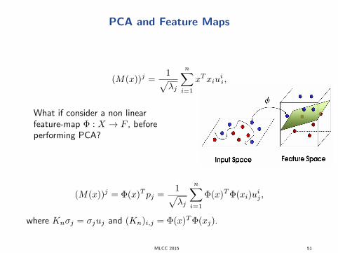
PCA and Feature Maps

(M(x))j =1√λj

n∑i=1

xTxiuij ,

What if consider a non linearfeature-map Φ : X → F , beforeperforming PCA?

(M(x))j = Φ(x)T pj =1√λj

n∑i=1

Φ(x)T Φ(xi)uij ,

where Knσj = σjuj and (Kn)i,j = Φ(x)T Φ(xj).

MLCC 2015 50

PCA and Feature Maps

(M(x))j =1√λj

n∑i=1

xTxiuij ,

What if consider a non linearfeature-map Φ : X → F , beforeperforming PCA?


n∑i=1

Φ(x)T Φ(xi)uij ,

where Knσj = σjuj and (Kn)i,j = Φ(x)T Φ(xj).

MLCC 2015 51

Kernel PCA


n∑i=1

Φ(x)T Φ(xi)uij ,

If the feature map is defined by a positive definite kernelK : X ×X → R, then

(M(x))j =1√λj

n∑i=1

K(x, xi)uij ,

where Knσj = σjuj and (Kn)i,j = K(xi, xj).

MLCC 2015 52

Wrapping Up

In this class we introduced PCA as a basic tool for dimensionalityreduction. We discussed computational aspect and extensions to nonlinear dimensionality reduction (KPCA)

MLCC 2015 53

Next Class

In the next class, beyond dimensionality reduction, we ask how we candevise interpretable data models, and discuss a class of methods based onthe concept of sparsity.

MLCC 2015 54

Documents

MLCC 2015 Dimensionality Reduction and PCAlcsl.mit.edu/courses/mlcc/mlcc2015/slides/MLCC_05_PCA.pdf · MLCC 2015 Dimensionality Reduction and PCA Lorenzo Rosasco UNIGE-MIT-IIT June