510 Chapter 12

of this dimensionality problem, regularization techniques such as SVD arealmost always needed to perform the covariance matrix inversion. Becauseit appears to be a fundamental property of hyperspectral data, however, thisdimensionality issue warrants further investigation, as it seems to indicatethat data representation is highly inefficient and overly sensitive to noise.

12.2 Dimensionality Reduction

From the geometric representation in Fig. 12.2, it is apparent from thelinear spectral mixing concept that signal content within hyperspectraldata is likely restricted to reside within a lower-dimensional subspace ofthe K-dimensional data space, where subspace dimensionality is dictatedby the number of spectrally distinct materials in the scene. Depending onscene complexity, this dimensionality could be small or quite large. In realsensor data, however, spectral measurements are corrupted by noise, whichis completely random and not restricted in the same manner. The reduceddimensionality of the information content within hyperspectral imagerycan be recognized by the high degree of correlation that typically existsbetween spectral bands.

For example, Fig. 12.4 illustrates three bands across the full spectralrange of a Hyperion satellite image over the intersection of two majorhighways in Beavercreek, Ohio. These bands capture some of thesame spatial features of the scene but also indicate significant spectraldifferences. The band-to-band correlation is modest, and each bandcarries a substantial amount of new information not contained withinthe others. On the other hand, there are other band combinations, suchas those depicted in Fig. 12.5, for which correlation is very high andeach band carries little additional information relative to the others. Toa large degree, the band combinations are redundant. This high degreeof correlation, or reduced inherent dimensionality, implies that the datacan be represented in a more compact manner. Transforming the datainto a reduced-dimensionality representation has multiple benefits. First,it limits the amount of data needed for processing and analysis, anobvious advantage where computer memory, network bandwidth, andcomputational resources are concerned. Additionally, representing thedata according to the primary signal components as opposed to thesensor spectral bands accentuates underlying material content, aidingvisualization and analysis. Finally, transforming to a lower-dimensionalsubspace should provide noise reduction, as this this process filters out thenoise power in the subspace that is removed.

12.2.1 Principal-component analysis

The principal-component transformation, commonly known as ei-ther principal-component analysis (PCA) (Schowengerdt, 1997) or the

Spectral Data Models 511

(a) (b) (c)

Figure 12.4 Three example bands from a Hyperion VNIR/SWIR hyperspectralimage over Beavercreek, Ohio, exhibiting modest spectral correlation: (a) 610 nm,(b) 1040 nm, and (c) 1660 nm.

(a) (b) (c)

Figure 12.5 Three example bands from a Hyperion VNIR/SWIR hyperspectralimage over Beavercreek, Ohio, exhibiting high spectral correlation: (a) 509 nm,(b) 610 nm, and (c) 2184 nm.

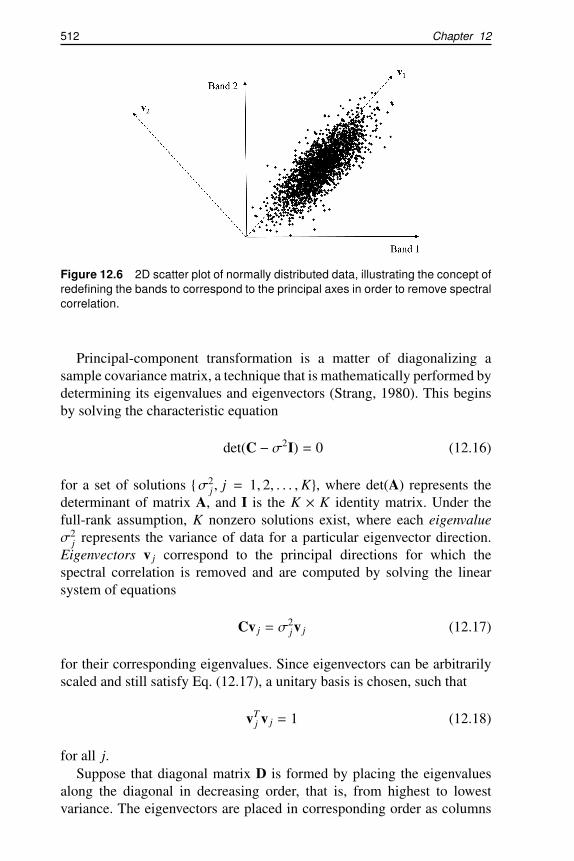
Karhunen–Loeve transformation (Karhunen, 1947; Loeve, 1963), ad-dresses the issue of spectral correlation and provides one basis for dealingwith data dimensionality. Assume for the moment that the inherent datadimensionality is actually K, such that the covariance matrix is full rankand therefore invertible. Spectral correlation manifests by nonzero, off-diagonal elements of the covariance matrix. Suppose that there was anotherset of orthogonal coordinate axes in the multidimensional space for whichthe covariance matrix was actually diagonal. If the data were transformedinto this new coordinate system, the spectral correlation between bandswould be removed. This is what the PCA transform attempts to perform;it is shown graphically for a simple 2D case in Fig. 12.6, where normallydistributed data are presented in the form of a scatter plot. Relative to thesensor spectral bands, the data exhibit a high degree of spectral correlation.However, correlation would be removed in this case if the bands were re-defined to correspond to the principal axes of the elliptically shaped scatterdistribution, denoted as v1 and v2 using dotted vectors.

512 Chapter 12

Figure 12.6 2D scatter plot of normally distributed data, illustrating the concept ofredefining the bands to correspond to the principal axes in order to remove spectralcorrelation.

Principal-component transformation is a matter of diagonalizing asample covariance matrix, a technique that is mathematically performed bydetermining its eigenvalues and eigenvectors (Strang, 1980). This beginsby solving the characteristic equation

det(C − σ2I) = 0 (12.16)

for a set of solutions {σ2j , j = 1, 2, . . . ,K}, where det(A) represents the

determinant of matrix A, and I is the K × K identity matrix. Under thefull-rank assumption, K nonzero solutions exist, where each eigenvalueσ2

j represents the variance of data for a particular eigenvector direction.Eigenvectors v j correspond to the principal directions for which thespectral correlation is removed and are computed by solving the linearsystem of equations

Cv j = σ2jv j (12.17)

for their corresponding eigenvalues. Since eigenvectors can be arbitrarilyscaled and still satisfy Eq. (12.17), a unitary basis is chosen, such that

vTj v j = 1 (12.18)

for all j.Suppose that diagonal matrix D is formed by placing the eigenvalues

along the diagonal in decreasing order, that is, from highest to lowestvariance. The eigenvectors are placed in corresponding order as columns

Spectral Data Models 513

of unitary eigenvector matrix V. It then follows from Eq. (12.17) that

CV = V D. (12.19)

Since the inverse of a unitary matrix is its transpose, it follows that

C = V DVT , (12.20)

which indicates that the linear transformation represented by eigenvectormatrix V diagonalizes the covariance matrix. Therefore, the principal-component transformation,

Z = VT X, (12.21)

represents a coordinate rotation to principal-component data matrix Z intoan orthogonal basis, such that the new principal-component bands are bothuncorrelated and ordered in terms of decreasing variance.

As an example of PCA, consider again the Hyperion Beavercreekimage shown in Figs. 12.4 and 12.5. Ranked eigenvalues of the samplecovariance matrix are displayed on a logarithmic scale in Fig. 12.7,where it is apparent that variance in the data is predominately capturedby a small set of leading principal-component directions. Figure 12.8provides the first three eigenvectors, while the principal-component bandimages, corresponding to the Hyperion data, are illustrated in Fig. 12.9.These images capture primary features of the original hyperspectral imagewith no spectral correlation. Generally, the first principal componentcorresponds to the broadband intensity variation, while the next fewcapture the primary global spectral differences across the image. Bycomparing a three-band false-color composite from these three principalcomponents with an RGB composite from the original 450-, 550-, and 650-nm bands (as illustrated in Fig. 12.10), the ability of the PCA to accentuatescene spectral differences is apparent. Statistically rare spectral featuresalong with sensor noise dominate the low-variance, trailing principalcomponents, three of which are illustrated in Fig. 12.11.

12.2.2 Centering and whitening

Several variations of PCA can be found in the literature and thereforewarrant some discussion. The first concerns removal of the sample meanvector m and scaling of the diagonalized covariance matrix D. Especiallywhen dealing with various target detection algorithms (described inthe next chapter), it is sometimes desirable to transform data into anorthogonal coordinate system centered within the data scatter as opposed

514 Chapter 12

Figure 12.7 Magnitude of the ranked eigenvalues of the Hyperion Beavercreekimage.

to the origin defined by the sensor data. This can be performed using theaffine transformation,

Z = VT (X −muT ) (12.22)

in place of the standard principal-component transformation given inEq. (12.21), or equivalently, by removing the sample mean vector mfrom all original spectral vectors prior to computing and performing theprincipal-component transformation. This is called centering, demeaning,or mean removal. Another variation is to use the modified transformationto scale the principal-component images such that they all exhibit unitvariance:

Z = D−1/2VT (X −muT ). (12.23)

This is referred to as whitening the data, and D−1/2 simply refers to adiagonal matrix for which the diagonal elements are all the inverse squareroot of the corresponding eigenvalues in D. To illustrate the differencebetween these variants of the principal-component transformation,Fig. 12.12 compares the transformed scatter plot from Fig. 12.6 in theprincipal component and whitened coordinate system. Data centering isperformed in each case.