CORE DISCUSSION PAPER9811

Mixing Mixed-Integer Inequalities

Oktay Gunluk1, and Yves Pochet2

January 1998

Abstract

Mixed-integer rounding (MIR) inequalities play a central role inthe development of strong cutting planes for mixed-integer programs.In this paper, we investigate how known MIR inequalities can be com-bined in order to generate new strong valid inequalities.

Given a mixed-integer region S and a collection of valid “base”mixed-integer inequalities, we develop a procedure for generating newvalid inequalities for S. The starting point of our procedure is to con-sider the MIR inequalities related with the base inequalities. For anysubset of these MIR inequalities, we generate two new inequalities bycombining or ”mixing” them. We show that the new inequalities arestrong in the sense that they fully describe the convex hull of a mixed-integer region associated with the base inequalities.

We also study some extensions of this mixing procedure, and dis-cuss how it can be used to obtain new classes of strong valid inequal-ities for various mixed-integer programming problems. In particular,we present examples for production planning, capacitated facility lo-cation, capacitated network design, and multiple knapsack problems.

Keywords: mixed integer programming, mixed integer rounding, Go-mory mixed integer cuts.

1School of ORIE, Cornell University, Ithaca, New York.2CORE and IAG, Universite Catholique de Louvain, Belgium.

The research of the first author was partially supported by a post-doctoral fellowship atCORE and NSF grant DMS-9527124 to Cornell University.

1 Introduction.

In the design phase of a cutting-plane (or branch-and-cut) algorithm forsolving a mixed-integer programming problem, z = min{cx : x ∈ S}, onevery important step is to define classes of strong valid inequalities for themixed-integer set S. In these algorithms, the linear programming relaxationof the problem is tightened by adding a selected subset of these inequali-ties, so-called cuts, to the formulation (see Nemhauser and Wolsey [16] fora general description of these algorithms). Among other critical factors, thesuccess of the algorithm depends on the quality of the tightened formulationas an approximation of the convex hull of S.

One way to generate such inequalities is to use general purpose cuttingplanes which do not require or exploit any a priori knowledge about thestructure of the problem at hand. The Gomory mixed-integer cuts (seeGomory [11]) which have been successfully used in a branch and cut frame-work (see Balas, Ceria, Cornuejols and Natraj [4]), or the disjunctive cuttingplanes (see Balas [2]) revisited and implemented as the equivalent lift andproject cuts (see Balas, Ceria, Cornuejols [3]) fall into this category.

Another possibility is to generate special purpose cutting planes thatare based on the polyhedral analysis of the problem formulation. Since itis difficult to capture the whole structure of the optimization problem inthese inequalities, the polyhedral analysis is usually performed on simplemathematical structures that are embedded in the problem formulation, orpossibly, on relaxations of the problem. This approach was first used tosolve pure 0-1 programs by considering the constraints of the formulationseparately and using facet inducing valid inequalities for the knapsack prob-lems associated with each constraint (see Crowder, Johnson and Padberg[10]) .

One important example of this approach is the mixed-integer rounding(MIR) inequality (see Nemhauser and Wolsey [15], and (3) below), which isderived from a single mixed-integer constraint. The MIR inequality can alsobe conseidered as a generalization of Chvatal’s integer rounding inequalityto the mixed-integer case (see Chvatal [8]). Based on the MIR inequal-ity, and motivated by the Gomory mixed-integer cuts, an MIR procedure is

This text presents research results of the Belgian Program on Interuniversity Poles ofAttraction initiated by the Belgian State, Prime Minister’s Office, Science Policy Pro-gramming. The scientific responsability is assumed by the authors.

2

derived for generating valid inequalities for any mixed-integer program. Byapplying this procedure a finite number of times (see Nemhauser and Wolsey[15]), one can generate all facet inducing valid inequalities for any mixed 0-1integer program. This result has been extended to general mixed-integerprograms by using a different recursion based on the so-called split cuts (seeCook, Kannan and Schrijver [9]).

The MIR inequality also provides a unifying framework for some of thefacet inducing inequalities for well-known mixed-integer programs. For ex-ample, the basic flow cover inequality (see Pagberg, Van Roy and Wolsey[17]), which is defined on a single flow conservation constraint with variableupper bounds on the flows, can be obtained as an MIR inequality from anappropriate relaxation of the mixed-integer set. Similarly, basic continuouscover inequalities for the 0-1 knapsack problem with a single continuous vari-able can be obtained as MIR inequalities (see Marchand and Wolsey [13]).For many other linear mixed-integer models, simple MIR inequalities havebeen derived to produce strong valid inequalities which have proven to becomputationally very effective (see [6], [7], [14], [18] and [20]).

Our primary objective in this paper is to contribute to the development of(general) techniques that can be used to generate new classes of strong validinequalities for mixed-integer programs. More specifically, we investigatehow to obtain new classes of valid inequalities by using or extending someknown classes of valid inequalities for a mixed-integer problem. One suchtechnique is the well-known lifting procedure which takes valid inequalitiesfor a polyhedral set , and extends them to valid inequalities for a supersetin a higher dimensional space (see Wolsey [21], Zemel [22], Gu, Nemhauserand Savelsbergh [12]).

Given the central role of the MIR inequalities in the development ofstrong cutting planes for mixed-integer programs, we investigate how togenerate new valid inequalities by combining known MIR inequalities.

We next formalize our approach and introduce the notation used through-out the paper. Given a mixed-integer region S ⊆ Rm1×Zm2 and a collectionof valid inequalities

f i(x) + Bgi(x) ≥ πi i ∈ I = {1, ...,m}, (1)

where B ∈ R1+ and πi ∈ R1, our purpose is to generate new valid inequalities

for S. We note that f i and gi can be non-linear and πi can be negative. In

3

particular, we concentrate on the case where the starting valid inequalities(1) satisfy f i(x) ≥ 0 and gi ∈ Z (not necessarily positive) for all x ∈ S. Inother words :

S ⊆ SR = { x ∈ Rm1 × Zm2 : f i(x) + Bgi(x) ≥ πi i ∈ I, (2)f i(x) ≥ 0, gi(x) ∈ Z i ∈ I }

We call the valid inequalities of the form (1) “base” inequalities, and thenew inequalities we generate are valid for the associated mixed-integer setSR. The starting point of our procedure is to consider the simple MIRinequality (3) associated with each base inequality. We refer the reader toNemhauser and Wolsey [15] and [16] for a more general definition of MIRinequalities. The simple MIR inequalities are derived as follows. For i ∈ I,let τ i =

⌈πi/B

⌉and γi = πi − (τ i − 1)B and note that τ i ∈ Z1, and

B ≥ γi > 0. We first re-write (1) as:

f i(x) ≥ πi −Bgi(x)= γi + B(τ i − gi(x)− 1)

and then, using f i(x) ≥ 0 for x ∈ S, we obtain the valid inequality

f i(x) ≥ γi(τ i − gi(x)). (3)

In the remainder of the text inequality (3) is called the MIR inequalityassociated with the base inequality (1). We next present a simple exampleto demonstrate how these inequalities work.

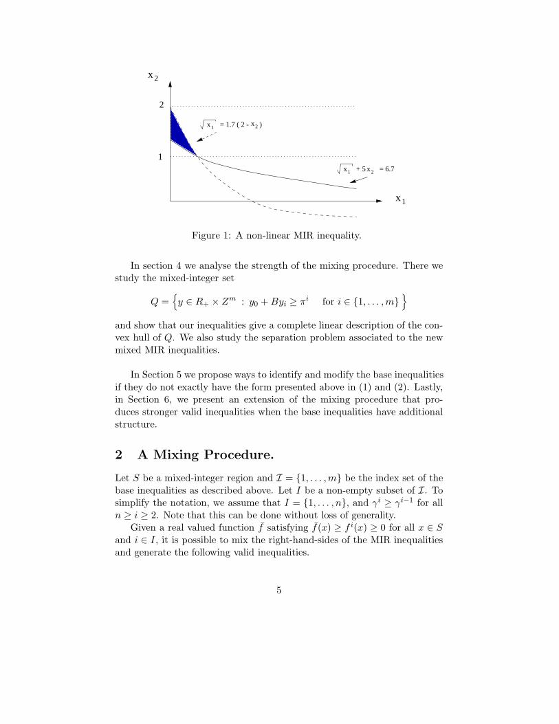
Example 1.1 Let√

x1 + 5x2 ≥ 6.7 be a base inequality where x ∈ R × Z.If we define f(x) =

√x1 and g(x) = x2, then τ = 2, γ = 1.7 and the related

MIR inequality is:√

x1 ≥ 1.7(2 − x2). In Figure 1, the shaded area corre-sponds to the set of points in R2 that satisfy the base inequality but violatethe MIR inequality.

The paper is organized as follows. In the next section, we present a“mixing” procedure that, for any subset of I, combines the related MIRinequalities and generates two new inequalities. The MIR inequalities canbe considered as a special case of this procedure (when the subset containsonly one inequality). In Section 3 we demonstrate the application of themixing procedure to various mixed-integer programming problems.

4

x1

x2

x2x1 + 5 = 6.7

x1x2

1

2

= 1.7 ( 2 - )

Figure 1: A non-linear MIR inequality.

In section 4 we analyse the strength of the mixing procedure. There westudy the mixed-integer set

Q ={y ∈ R+ × Zm : y0 + Byi ≥ πi for i ∈ {1, . . . ,m}

}

and show that our inequalities give a complete linear description of the con-vex hull of Q. We also study the separation problem associated to the newmixed MIR inequalities.

In Section 5 we propose ways to identify and modify the base inequalitiesif they do not exactly have the form presented above in (1) and (2). Lastly,in Section 6, we present an extension of the mixing procedure that pro-duces stronger valid inequalities when the base inequalities have additionalstructure.

2 A Mixing Procedure.

Let S be a mixed-integer region and I = {1, . . . ,m} be the index set of thebase inequalities as described above. Let I be a non-empty subset of I. Tosimplify the notation, we assume that I = {1, . . . , n}, and γi ≥ γi−1 for alln ≥ i ≥ 2. Note that this can be done without loss of generality.

Given a real valued function f satisfying f(x) ≥ f i(x) ≥ 0 for all x ∈ Sand i ∈ I, it is possible to mix the right-hand-sides of the MIR inequalitiesand generate the following valid inequalities.

5

Theorem 2.1 The following two inequalities

f(x) ≥n∑

i=1

(γi − γi−1)(τ i − gi(x)) (4)

and

f(x) ≥n∑

i=1

(γi − γi−1)(τ i − gi(x)) + (B − γn)(τ1 − g1(x)− 1) (5)

where γ0 = 0, are valid for S.

Proof. For any fixed x ∈ S, define β = maxi∈I{τ i− gi(x)} and v = max{i ∈I : β = τ i − gi(x)}. If β ≤ 0 then the right-hand sides of (4) and (5)are at most zero and the inequalities are valid. Therefore we assume thatβ = τv − gv(x) ≥ 1.

Using β ≥ τ i − gi(x) for all i ≤ v and β ≥ τ i − gi(x) + 1 for i > v, wewrite

n∑i=1

(γi − γi−1)(τ i − gi(x)) ≤v∑

i=1

(γi − γi−1)(β) +n∑

i=v+1

(γi − γi−1)(β − 1)

= (γv)(β) + (γn − γv)(β − 1)= γn(β − 1) + γv

≤ B(β − 1) + γv

≤ f v(x)≤ f(x).

Also note that the above argument is still valid when v = n. This provesthe validity of (4). To show the validity of (5), we similarly write

n∑i=1

(γi − γi−1)(τ i − gi(x)) + (B − γn)(τ1 − g1(x)− 1)

≤v∑

i=1

(γi − γi−1)(β) +n∑

i=v+1

(γi − γi−1)(β − 1) + (B − γn)(β − 1)

= (γv)(β) + (B − γv)(β − 1) = B(β − 1) + γv

≤ f(x).

Note that when |I| = 1, and f = f1, the related mixed inequality (4)gives the simple MIR inequality (3) and inequality (5) gives the original

6

base inequality (1). We next give a small example to demonstrate how themixing procedure works.

Example 2.2 Let S = {(x, y) ∈ R1+×Z2 : (a)x1+10y1 ≥ 3, (b)x1+10y2 ≥

5} and S+ = S∩{(x, y) ∈ R1+×Z2

+}. If we write the MIR inequalities relatedwith (a) and (b), we obtain: (a′) : x1 ≥ 3(1 − y1) and (b′) : x1 ≥ 5(1 − y2)and when we apply the mixing procedure with f = f1 = f2 = x1, B = 10,and gi = yi, the resulting inequality (4) is

x1 ≥ 3(1 − y1) + 2(1 − y2). (ab′)

A complete polyhedral description of S+ is given by conv(S+) = {(x, y) ∈R1

+ ×R2+ : (a′), (b′), (ab′)}.

Similarly, the inequality (5) obtained by mixing the MIR inequalities (a′)and (b′) is

x1 ≥ 3(1 − y1) + 2(1 − y2) + 5(−y1) (ab′′)

and conv(S) = {(x, y) ∈ R1+ ×R2 : (a), (b), (a′), (b′), (ab′), (ab′′)}.

The strength of inequalities (4) and (5) clearly depends on how f ischosen. Note that f satisfies f(x) ≥ f∗(x) for all x ∈ S, where f∗(x) =maxi∈I{f i(x)}. If it is practical, one should use f = f∗ in (4) and (5),but this might be undesirable since in general f∗ would not be a smoothfunction.

3 Examples.

In this section, we consider the application of the mixing procedure to somewell known mixed-integer programming problems. We describe how to de-rive known classes of valid inequalities using the procedure. We also generatenew valid inequalities for these problems.

In fixed charge capacitated network flow problems (such as lot-sizing,facility location and network design) a possible way to construct the baseinequalities (1) is to aggregate flow balance constraints over a set of con-nected nodes in the underlying flow graph. This gives constraints of theform

∑j∈N1

xj −∑

j∈N2

xj = d ,

7

which can be relaxed to ∑j∈N1

xj ≥ d .

Now, partitioning N1 into F ∪ G and using the variable upper bound con-straints (or capacity constraints), xj ≤ ujyj for j ∈ G , yields the baseinequality

∑j∈F

xj +∑j∈G

ujyj ≥ d .

This general principle for constructing base inequalities and the corre-sponding mixed inequalities (4) and (5) is now illustrated on several appli-cations.

3.1 Production Planning.

The constant capacity single item lot-sizing problem (LCC) consists of aplanning horizon n (i.e. a set of periods {1, . . . , n}) with known demanddt and production capacity C per period , 1 ≤ t ≤ n. The objective isto find a production plan meeting the demands (without backlogging) andminimizing total production costs (unit production costs and setup costs)and inventory costs. Its feasible set XLCC is defined by

XLCC ={(x, s, y) ∈ Rn

+ ×Rn+1+ ×Bn :st−1 + xt = dt + st for 1 ≤ t ≤ n

xt ≤ Cyt for 1 ≤ t ≤ n

s0 = sn = 0}

where xt, st, yt represent respectively the production, inventory and binarysetup variables in period t. Whenever there is a setup in period t (i.e.yt = 1), the production capacity is C.

For a fixed time period k ≥ 1, let F ∪G be a partition of N = {k, . . . , n}such that k ∈ G. We can define a base inequality for each period t ∈ N byaggregating the flow balance constraints over the periods k up to t. Thisgives

sk−1 +∑

j∈F∩{k,...,t}xj +

∑j∈G∩{k,...,t}

Cyj ≥t∑

j=k

dj .

It can be checked that by using the mixing procedure for any subsetI ⊆ {t : t + 1 ∈ G} ∪ {n} of these base inequalities, one gets, as inequalities

8

of type (4), precisely the so-called (k, l, S, I) inequalities (see [18]) with thefunction f(x) defined as

f(x) = sk−1 +∑

j∈F∩(∪t∈I{k,...,t})xj .

Pochet and Wolsey ([18]) show that (k, l, S, I) inequalities generate allfacets of conv(XLCC ) of the form

sk−1 +∑j∈F

xj +∑j∈G

αjyj ≥ π0

for all 2 ≤ k ≤ l ≤ n and all partitions F,G of {k, . . . , l}. Moreover, it isknown that adding only a subset of these inequalities (those with F = ∅,G = {k, . . . , l}) suffices to solve problem LCC by linear programming (with-out enumeration) when the objective function satisfies the Wagner-Whitinassumption (see Pochet and Wolsey [19]). The so-called (l, S) inequalitiesknown to describe the convex hull of feasible solutions of the uncapacitated(i.e. C = ∞) single item lot sizing problem (see Barany, Van Roy andWolsey [5]) can also be obtained by the mixing procedure.

3.2 Capacitated Facility Location.

The capacitated facility location problem consists of a set M = {1, . . . ,m}of potential depots with capacity Cj, 1 ≤ j ≤ m, and a set N = {1, . . . , n}of clients with demand dk, 1 ≤ k ≤ n. The objective is to decide whichdepots to open and to assign demands to open depots in order to minimizedepot installation costs and distribution costs. Its feasible set XCFL can bedefined as

XCFL ={(v, y) ∈ Rm×n

+ ×Bm :m∑

j=1

vjk = dk for 1 ≤ k ≤ n

n∑k=1

vjk ≤ Cjyj for 1 ≤ j ≤ m

vjk ≤ dkyj for 1 ≤ j ≤ m , 1 ≤ k ≤ n}

where the variable vjk represents the amount of demand dk delivered fromdepot j and the binary variable yj indicates whether or not depot j is open.

9

For any subset K ⊆ N of clients, we can construct a flow cover relaxationXFC

K of XCFL as

XFCK =

{(w, y) ∈ Rm

+ ×Bm :m∑

j=1

wj =∑

k∈K dk

wj ≤ Cjyj for 1 ≤ j ≤ m}

by defining the projected variable wj as wj =∑

k∈K vjk. When the capacitiesare equal (i.e. Cj = C for all j), Padberg, Van Roy and Wolsey [17] provethat the convex hull of this relaxation XFC

K is defined by the MIR inequalities(3) corresponding to the set of base inequalities

∑j∈M\S

wj + C∑j∈S

yj ≥∑k∈K

dk ,

for S ⊆ M = with |S| ≥ d∑k∈K dk/Ce.

Therefore, for i = 1, . . . , r, we can choose sets Si ⊆ M , Ki ⊆ N andmix the corresponding base inequalities. The (k, l, S, I) based inequalitiesdefined in Aardal, Pochet and Wolsey [1] can be obtained by mixing thesebase inequalities, when {Si,Ki} form a ”nested” family (i.e. K1 ⊂ K2 ⊂. . . ⊂ Kr and S1 ⊂ S2 ⊂ . . . ⊂ Sr). The corresponding mixed inequalitiesare typically strong (defining facets or high dimensional faces).

We next give an example of a facet defining mixed inequality, for thecase of different capacities Cj, which does not correspond to such a nestedfamily of base inequalities. This example inequality could also be derivedas a lifted flow cover inequality by constructing an appropriate relaxation ofXCFL (see [17]).

Example 3.1 Consider the following instance of XCFL with m = 5 depotsof different capacity C = (4, 10, 10, 10, 50) and n = 3 clients whose demandsare d = (6, 9, 7).We define a first base inequality by S = M \ {5} and K = N

(v51 + v52 + v53) + 4y1 + 10y2 + 10y3 + 10y4 ≥ 22 .

¿From this base inequality, we define two other (relaxed) base inequalities byreplacing the term 4y1 by its upper bound 4 in the first inequality, and by

10

10y1 in the second inequality:

(v51 + v52 + v53) + 10y2 + 10y3 + 10y4 ≥ 18 , and

(v51 + v52 + v53) + 10y1 + 10y2 + 10y3 + 10y4 ≥ 22 .

It can be checked that the mixed inequality (4) defined by

(v51 + v52 + v53) ≥ 2(3 − y1 − y2 − y3 − y4) + 6(2− y2 − y3 − y4)

defines a facet of this instance of conv(XCFL).

3.3 Capacitated Network Design.

We next study the capacity expansion problem (CEP) that arises in telecom-munication network design. The problem data consists of an undirectedgraph G = (V,E) with existing capacities ke ≥ 0 for e ∈ E, and point-to-point traffic demands {tij} to be routed through the network. Additionalcapacity has to be installed on edges in integer multiples of several modu-larities (corresponding to different technologies) in order to support the flowon the edges. The objective is to minimize the total routing and capacityinstallation cost. For simplicity, we consider the case when there is only onebatch size (technology).

If we define K = {i ∈ V :∑

j∈V tij > 0} , the set of feasible solutionsXCEP is defined by

XCEP ={(f, y) ∈ R

2|K| |E|+ × Z

|E|+ :

∑{i,j}∈E

fkji −

∑{i,j}∈E

fkij = tki for i ∈ V, k ∈ K \ {i}

∑k∈K

fkij ≤ Cye + ke for e = {i, j} ∈ E

∑k∈K

fkji ≤ Cye + ke for e = {i, j} ∈ E

}

where fkij corresponds to the flow of commodity k (i.e. traffic with origin

at node k) on the directed arc from i to j and ye represents the number ofbatches of capacity C installed on edge e = {i, j}. The total flow on arc (i, j)cannot exceed the capacity Cye installed on edge e plus the existing capacityke. The first set of equalities in the above formulation simply represents theflow balance constraints.

11

In [6] Bienstock and Gunluk present several classes of facet defininginequalities for conv(XCEP ). Most of their inequalities are based on theso-called cut-set and flow-cut-set inequalities. For any S ⊂ V , let δ(S) ∈ Ebe the set of edges with one end in S and the other in V \ S. It is easy tosee that the cut-set inequality

∑e∈δ(S)

ye ≥⌈T (S)

C

⌉

where T (S) = max{∑i∈S

∑j∈V \S tij ,

∑i∈V \S

∑j∈S tij}−∑

e∈δ(S) ke, is validfor XCEP .

It is also possible to construct base inequalities of the form (1) by parti-tioning δ(S) into E1 ∪E2 and selecting a subset Q ⊆ (K ∩ S). If we let A1

denote the set of directed edges obtained by orienting the edges in E1 awayfrom S, we can write the following valid inequality:

∑(i,j)∈A1

∑k∈Q

fkij + C

∑e∈E2

ye ≥∑k∈Q

∑j∈V \S

tkj −∑

e∈E2

ke.

The flow-cut-set inequalities are precisely the MIR inequalities (3) con-structed from this base inequality.

It is also possible to mix these base inequalities to obtain new validinequalities. We next give an example of a fractional solution feasible tothe formulation consisting of the linear programming relaxation of XCEP

augmented by all cut-set and flow-cut-set inequalities. This fractional pointviolates a mixed inequality of the form (4).

Example 3.2 Consider the following example with two nodes (representingS and V \ S), and two commodities a and b with origin in S. The batchcapacity is C = 10 and the total demand for a and b in V \ S is 17 and 8,respectively. The directed cut from S to V \ S contains three arcs denotedby e = 1, 2 and 3. The existing capacities are k = (0, 10, 0). The fractionalpoint given in Table 1 satisfies all cut-set and flow-cut-set inequalities.

edges e ye fae f b

e

1 3/4 1/4 19/42 0 6/4 4/43 7/4 61/4 9/4

Table 1: A fractional solution

12

Consider the following two base inequalities with E2 = {3}, Q = {a} andE2 = {1, 3}, Q = {a, b} :

fa1 + fa

2 + 10y3 ≥ 17 ,

fa2 + f b

2+ 10y1 + 10y3 ≥ 25

and note that their corresponding MIR inequalities (3) are satisfied at equal-ity :

fa1 + fa

2 = 7/4 ≥ 7(2− y3) = 7/4 ,

fa2 + f b

2 = 10/4 ≥ 5(3− y1 − y3) = 5/2.

If we mix these two inequalities, the resulting inequality

fa1 + fa

2 + f b2 = 11/4 ≥ 5(3− y1 − y3) + 2(2− y3) = 5/2 + 2/4 = 12/4

is violated by the fractional point.

3.4 Multiple Knapsack.

As a final example we illustrate how the mixed inequalities generate facets ofpure integer problems, and introduce the extensions of the mixed inequalitiesthat will be presented in Section 5.

Example 3.3 Consider the following feasible set X which consists in theintersection of two integer knapsack constraints.

X = {x ∈ Z5+ : x1 + 3x2 + 10x4 ≥ 25 , and x1 + 2x3 + 10x5 ≥ 37}.

If we define two base inequalities by f1(x) = x1 + 3x2, g1(x) = x4,π1 = 25, f2(x) = x1 + 2x3, g2(x) = x5, π2 = 37, and B = 10, then thecorresponding mixed inequalities, respectively of type (4) and (5)

x1 + 3x2 + 2x3 ≥ 5(3 − x4) + 2(4 − x5) (6)x1 + 3x2 + 2x3 ≥ 5(3 − x4) + 2(4 − x5) + 3(2− x4) (7)

generate facets of conv(X).

If we modify the set X into X ′ defined by

X ′ = {x ∈ Z5+ : x1 + 3x2 + 10x4 ≥ 25 , and x1 + 2x3 + 8x5 ≥ 31}.

then the above mixed inequality (6) is still valid and generates a facet ofconv(X ′). We will see in the next section that this inequality can be obtainedby taking two different values for B, namely B1 = 10 and B2 = 8.

13

4 The Strength of the Mixing Procedure

We analyse now the strength of the valid inequalities (4) and (5) generatedby the mixing procedure. Our main result, Theorem 4.5 established inSubsection 4.2, shows that the mixing procedure suffices to obtain a completelinear description of the convex hull of the mixed-integer region Q definedby the following set of base inequalities:

Q ={y ∈ R+ × Zm : y0 + Byi ≥ πi for i ∈ {1, . . . ,m}

}

In subsection 4.1, we start by establishing an intermediate result, namelyCorollary 4.4, needed to prove our main result. We end this section with thestudy of the separation problem associated with the mixed MIR inequalities(4) and (5).

4.1 The Coefficient Polyhedron PC .

It is possible to generalize (4) and (5) and write valid inequalities of theform f(x)+α ≥ ∑

i∈I δi(τ i−gi(x)) when α and δ satisfy certain properties.Without loss of generality, we again write I = {1, . . . ,m} with γi ≥ γi−1

for all m ≥ i ≥ 2.

Lemma 4.1 The following inequality is valid for S

f(x) + α ≥∑i∈I

δi(τ i − gi(x)) (8)

provided:(i) (δ, α) ∈ PC , where

PC ={(δ, α) ∈ R

|I|+1+ :

∑i∈I

δi ≤ B

∑j≤i

δj ≤ α + γi, for all i ∈ I}

(ii) f(x) ≥ f i(x) for all x ∈ S and for all i ∈ I with δi > 0.

Proof. Similar to the proof of Lemma 2.1.

Note that the coefficients (δ, α) in the inequalities (4) or (5) belong tothe coefficient polytope PC , and inequality (8) with (δ, α) ∈ PC appearsthus to be a generalization of (4) and (5). We will show that, although

14

inequality (8) seems to be more general, any inequality of the form (8) with(δ, α) ∈ PC is equivalent to or is dominated by an inequality (4) or (5).

Lemma 4.1 defines sufficient conditions on the coefficients (δ, α) for in-equality (8) to be valid for S. The following remark states the properties ofthe mixed-integer region S under which these conditions are also necessary.

Remark 4.2 Let (δ, α) ∈ R|I|+1+ with

∑i∈I δi ≤ B. Furthermore, let f be

a function satisfying f(x) ≥ f i(x) for all x ∈ S and for all i ∈ I = {i ∈ I :δi > 0}.If for all t ∈ I there exists a point xt ∈ S with:

(i) τ t − gt(xt) = 1 for i = 1, ..., t and τ t − gt(xt) = 0 for i = t + 1, ...,m,and,

(ii) f(xt) = γt,

then, (8) is valid for S if and only if (δ, α) ∈ PC .

In the above remark, note that if points xt exist for all t ∈ I, then the mixingprocedure to obtain inequality (4) can also be viewed as a sequential lift-ing procedure, starting from a simple MIR inequality, and where functions(τ i − gi(x)) are lifted sequentially instead of variables. Similarly, if thereexists y ∈ S with τ1 − g1(y) = 2, τ t − gt(y) = 1 for t = 2, · · · ,m , andf(y) = γ1 + B, then inequality (5) can be obtained from (4) by lifting thefunction (τ1 − g1(x)− 1).

We show now that inequalities (4) and (5) contain all important in-equalities of the form (8) with (δ, α) ∈ PC . Let p = (δ, α) be an arbitrary,non-extreme point of the coefficient polyhedron PC and consider the associ-ated valid inequality (8). Since p can be expressed as a convex combinationof other points in PC , that is, p = εp1 + (1− ε)p2 for some p1, p2 ∈ PC andsome ε ∈]0, 1[, the inequality generated by p can also be obtained by sim-ply combining the inequalities associated with p1 and p2. We are thereforemainly interested in valid inequalities generated by the extreme points andextreme directions of PC , and next we present a complete characterizationof the extreme points.

Lemma 4.3 Let p = (δ, α) be an arbitrary, non-zero extreme point of PC ,and define I = {i ∈ I : δi > 0} = {i1, i2, . . . , in} with i1 < i2 < . . . < in.The extreme point p = (δ, α) is characterized by:

α ∈ {0, B − γin}

15

δi1 = γi1 + α

δij = γij − γij−1 for j = 2, . . . , nδi = 0 for i ∈ I \ I

Proof. Note that the only extreme point of PC with δ = 0 is the origin,and thus |I| > 0. First we show that if p is an extreme point of PC ,then

∑j≤i δ

j = α + γi for all i ∈ {i1, i2, . . . , in−1}. Assume∑

j≤ikδj <

α + γik for some 1 ≤ k < n. In this case, p can be expressed as a convexcombination of two other points in PC . The first point p1 is obtained fromp by simultaneously increasing γik and decreasing γik+1 by a small ε >0. Similarly, p2 is obtained from p by simultaneously decreasing γik andincreasing γik+1 by the same ε. Clearly p1, p2 ∈ PC , and p = 1/2p1 + 1/2p2.

Next, consider in and assume∑

j≤in δj < α + γin . If∑

i∈I δi < B, thentwo points p1, p2 ∈ PC can be obtained by simply increasing and decreasingδin by a small ε > 0 and p = 1/2 (p1+p2). On the other hand, if

∑i∈I δi = B,

then we have∑

i∈I δi = B < α+γin and thus α > 0. In this case, we obtainp1 ∈ PC by simultaneously increasing δi

1 and α, and decreasing δin by a small

ε > 0. The second point p2 ∈ PC is obtained by decreasing δi1 and α, and

increasing δin by the same ε > 0, and p = 1/2p1 + 1/2p2. (If |I| = 1, we

construct p1 and p2 by perturbing α only.)We therefore established that

∑j≤i δ

j = α + γi for all i ∈ I which, inturn, implies that α =

∑i∈I δi−γin and thus α ≤ B−γin . Finally, we need

to show that α is either zero or B − γin . Assume 0 < α < B − γin , andtherefore

∑i∈I δi < B. We construct the following two points: p1 is obtained

from p by increasing α and γi1 by ε > 0, and p2 is obtained by decreasing αand γi1 by the same ε. Clearly p1, p2 ∈ PC , and p = 1/2 (p1 + p2).

Although inequalities of the form (8) appear to be more general thanthe valid inequalities generated by the mixing procedure, any inequalitygenerated by an extreme point of PC coincides with one of (4) or (5). Moreprecisely, for an inequality (8) associated with an extreme point of PC , weconstruct I by choosing all i ∈ I with δi > 0. If α is zero, then the inequalitycoincides with (4), and if α is positive, it coincides with (5). Since the onlyextreme direction of PC is (δ, α) = (0, 1), we have the following corollary:

Corollary 4.4 Inequality (8) generated by (δ, α) ∈ PC is equivalent to ordominated by a positive combination of inequalities (4) and (5).

16

4.2 A Related Mixed-integer Set.

Given a function f , let I = {i ∈ I : f(x) ≥ f i(x) for all x ∈ S}. Theinequalities produced by the mixing procedure are actually valid for thefollowing continuous relaxation of the mixed-integer set S:

SR(I) ={x ∈ Rm1+m2 : f(x) ≥ 0

gi(x) ∈ Z for i ∈ I

f(x) + Bgi(x) ≥ πi for i ∈ I}.

Furthermore, since we are not considering the interdependencies amongfunctions gi, i ∈ I, or f , we are essentially producing valid inequalitiesfor the following mixed-integer set:

QI ={y ∈ R+ × Z |I| : y0 + Byi ≥ πi for i ∈ I

}.

Note that if an inequality βy ≥ θ is valid for QI , then

β0f(x) +∑i∈I

βigi(x) ≥ θ

is valid for SR(I) and thus also valid for S.We next show that inequalities (4) and (5), or equivalently inequalities

of the form (8), are sufficient to obtain a complete polyhedral descriptionof Q ≡ QI . To study Q, we use the same notation as before. For i ∈ I ={1, . . . ,m}, we define τ i =

⌈πi/B

⌉and γi = πi − (τ i − 1)B with γi ≥ γi−1.

We use {i1, i2, . . . , i|I|} to denote the members of any subset I ⊆ I andassume i1 < i2 < . . . < i|I|. We also define γi0 = 0.

Theorem 4.5

conv(Q) ={y ∈ R+ ×R|I| :

y0 ≥|I|∑

j=1

(γij − γij−1)(τ ij − yij) for all I ⊆ I,

y0 ≥|I|∑

j=1

(γij − γij−1)(τ ij − yij) + (B − γi|I|)(τ i1 − yi1 − 1) for all I ⊆ I}

Proof. Let βy ≥ θ be an arbitrary valid inequality for Q with β 6= 0. UsingCorollary 4.4, it suffices to show that the inequality can be re-written as:

y0 + α ≥∑i∈I

δi(τ i − yi) (9)

17

for some (δ, α) ∈ PC .Consider a valid inequality βy ≥ θ and note that for any y ∈ Q, and

i ∈ {0, 1, . . . ,m}, one can obtain a new point y ∈ Q by increasing thei’th component of y by one. This implies that β ≥ 0. Also note thatpµ = (µB, τ1−µ, τ2−µ, . . . , τm−µ) ∈ Q for any non-negative integer µ andif β0 = 0, then for some µ ∈ Z+, pµ violates the inequality. Therefore, weestablished that any inequality βy ≥ θ can be re-written as (9) and δi ≥ 0for all i ∈ I. Finally, p0 ∈ Q implies that α ≥ 0.

Now we need to show that (i)∑

i∈I δi ≤ B and (ii)∑

j≤i δj ≤ α + γi,

for all i ∈ I. First note that pµ ∈ Q for all µ ∈ Z+ implies that µB + α ≥∑i∈I δiµ for all µ ∈ Z+, and thus

∑i∈I δi cannot exceed B. Finally, for

i ∈ I, let qi ∈ R|I|+1 be such that qi0 = γi and qi

k = τ i − 1 for all 1 ≤ k ≤ iand qi

k = τ i for all i < k ≤ m. Since qi ∈ Q for i ∈ I, the inequality has tosatisfy (ii) for all i ∈ I and the proof is complete.

If we define Q+ to be the intersection of Q with the non-negative orthant:

Q+ ={y ∈ R+ × Z

|I|+ : y0 + Byi ≥ πi for i ∈ I

},

then it is possible to show that the mixed inequalities (4) and (5) are stillsufficient for a complete linear decription of the convex hull of Q+. In otherwords:

conv(Q+) = conv(Q) ∩R|I|+1+ .

This requires minor modifications in the proof of Lemma 4.5. In this case,inequality (5) becomes redundant unless the set I ⊆ I has yi1 < τ i1 − 1for some y ∈ Q+ (see Example 2.2). We also note that an alternative proofof Theorem 4.5 can be adapted from the study of the capacitated lot-sizingpolyhedron in [19].

4.3 Finding Violated Inequalities.

Given a point x ∈ X, we next address the (separation) problem of finding a(δ, α) ∈ PC that maximizes the right-hand-side of:

f(x) ≥∑i∈I

δi(τ i − gi(x))− α. (10)

Let hi(x) = (τ i− gi(x)) and (δ, α) be such that it has the minimum numberof non-zero components. Due to the structure of the extreme points ofPC , it is easy to see that α is non-zero if and only if maxj∈I{hj(x)} > 1.

18

Similarly, for all i ∈ I, δi is non-zero if and only if (i) hi(x) > hj(x) for allj > i, (ii) hi(x) > maxj∈I [hj(x)− 1], and (iii) hi(x) > 0.

Using the above observations and the correspondence between extremepoints of PC and subsets of I given in Lemma 4.3, we next present analgorithm that constructs a set I ⊆ I and fixes the value of α. The valuesδi for i ∈ I are then fixed according to Lemma 4.3.

1. Order the base inequalities in non-increasing order of γi and set hmax =maxj∈I{hj(x)}. If hmax ≤ 0, then (δ, α) = 0, stop.

2. Set best = max{0, hmax − 1}, I = ∅ and start from the top of the list,

3. Scan the list until hi(x) > best or the list is exhausted.

4. If the list is not finished, set I = I ∪ {i} and best = hi(x), go to step3.If the list is finished, goto step 5.

5. If hmax > 1, fix α to B −maxj∈I{γj}.Fix it to zero otherwise. Return the set I and α

We also note that finding a most violated inequality of the form (8) (or(4)-(5)) is more complicated than simply maximizing the right-hand-side of(10). This is mainly because the choice of the set I may in turn affect thechoice of f and thus the value of f(x). If f(x) does not depend on the setI, which is the case for the mixed integer set Q, then the above proceduregives an exact separation algorithm. Otherwise, it should be considered asa heuristic. We next give an example to emphasize this point.

Example 4.6 Let P ′ = {x ∈ R2+, y ∈ Z2

+ : (1)x1 +10y1 ≥ 3, (2)x1 +10y2 ≥5, (3) x1 + x2 + 10y3 ≥ 9} and p = (x1, x2, y1, y2, y3) = (3, 9, 0, 0.4, 0.5). Ifwe apply the above procedure with gi = yi, we obtain I = {1, 2, 3}, α = 0,and the resulting inequality of type (4) is:

f(p) ≥ 3(1− y1) + 2(1− y2) + 4(1 − y3). (c)

Since we are mixing all three inequalities, f is (at least) x1 + x2 and thusp satisfies (c). However p does not satisfy (ab′) of Example 2.2 and thusp /∈ conv(P ′).

19

5 Variations.

In this section we show how the mixing procedure can be applied when someof the base inequalities do not have the form (1) or do not satisfy (2).

First we consider the case when f i(x) ≥ 0 does not hold for a baseinequality i ∈ I. In this case the MIR inequality (3) is not valid. If f i(x)can be bounded from below, i.e. if we have f i(x) ≥ LBi, then we rewritethe related inequality as follows:(

f i(x)− LBi)

+ Bgi(x) ≥ πi − LBi (11)

so that f i(x) = f i(x) − LBi ≥ 0. It is now possible to apply the mixingprocedure, with f i(x) and by computing τ i and γi using the new right-hand-side πi − LBi, to obtain valid inequalities of type (4) and (5).

Another possibility is to have base inequalities of the form,

f i(x) + Bigi(x) ≥ πi

where Bis are not necessarily the same for all i ∈ I. In this case, we defineτ i =

⌈πi/Bi

⌉and γi = πi − (τ i − 1)Bi, and check if B = mini∈I{Bi} ≥

γ = maxi∈I{γi} holds. If B ≥ γ, then we can apply the mixing procedureand the resulting inequality (4) is valid for S (the proof is similar to thatof Lemma 2.1.) On the other hand if B < γ, it is possible to relax thebase inequalities with small Bi’s by replacing Bi with γ and then apply themixing procedure to obtain a valid inequality of type (4). Another possibleapproach is to “scale” the base inequalities so as to increase B or to decreaseγ.

Let αi > 0 be the scaling coefficients for i ∈ I, and consider the scaledbase inequality of type (1)

αif i(x) + (αiBi)gi(x) ≥ αiπi (12)

and the related MIR inequality,

αif i(x) ≥ γi(τ i − gi(x)) = αiγi(τ i − gi(x))

where τ i =⌈αiπi/αiBi

⌉=

⌈πi/Bi

⌉= τ i and γi = αiπi − (τ i − 1)αiBi =

αi(πi − (τ i − 1)Bi) = αiγi. Using scaled inequalities (12) as the base set,we can apply the mixing procedure if mini∈I{αiBi} ≥ maxi∈I{αiγi} holds,and obtain new inequalities of type (4).

We note that this idea can also be helpful if one can use the same f afterscaling some inequalities up, or if one can find a better f after scaling someinequalities down. This is illustrated in the next example.

20

Example 5.1 Consider mixing the following inequalities where x1, x2 ∈ R1+

and x3, x4 ∈ Z1:

x1 + 2x2 + 7x3 ≥ 153x1 + 5x2 + 10x4 ≥ 14

and note that if we set g1(x) = x3 and g2(x) = x4, then τ1 = 3, τ2 = 2,γ1 = 1, and γ2 = 4. Since B ≥ γ, we can apply the mixing procedure withf(x) = 3x1 + 5x2 to obtain,

3x1 + 5x2 ≥ (3− x3) + 3(2− x4). (13)

It is also possible to apply the mixing procedure after scaling the first in-equality by 5/2 and obtain

3x1 + 5x2 ≥ (5/2)(3 − x3) + (3/2)(2 − x4).

which is stronger than (13) when 3− x3 > 2− x4.

6 Mixing Independent Constraints.

In the examples presented in Section 3, the functions f i were always “de-pendent” with respect to f in the sense that, due to their common terms,we did not have f(x) ≥ f i(x) + f j(x) for two different i, j ∈ I. However,when this occurs, inequalities assocated with i and j can be treated as “in-dependent” base inequalities and the mixed inequality (4) can be tightenedto give a stronger inequality. Before formalizing this idea, we first presentan example.

Example 6.1 Consider a 5 depots, 3 clients instance of the capacitatedfacility location problem (CFL) with demands d = (9, 2, 15) and capacityC = 10. We take the three base inequalities

v21 + v31 + v41 + v51 + 10y1 ≥ 9 (S = K = {1})v13 + v23 + v53 + 10y3 + 10y4 ≥ 15 (S = {3, 4},K = {3})

v51 + v52 + v53 + 10y1 + 10y2 + 10y3 + 10y4 ≥ 26 (S = {1, 2, 3, 4},K = {1, 2, 3})Combining these base inequalities using the mixing procedure of section 2,we obtain

f(x) = v13 + (v21 + v23) + v31 + v41 + (v51 + v52 + v53)≥ 5(2 − y3 − y4) + 1(3 − y1 − y2 − y3 − y4) + 3(1− y1).

21

Now, as f(x) ≥ f1(x)+f2(x) = v13 +(v21 +v23)+v31 +v41 +(v51 +v53),the first two base inequalities can be treated as independent, and the followinginequality

f(x) ≥ f1(x) + f2(x) ≥ 5(2− y3 − y4) + 9(1 − y1)

is valid. Since the third base inequality is not independent of the other two(i.e. f(x) 6≥ f1(x)+f3(x) and f(x) 6≥ f2(x)+f3(x)) , when introducing thisthird inequality into the mixed inequality we use the basic mixing procedure.This gives the following inequality

f(x) ≥ 5(2− y3 − y4) + (6− 5)(3 − y1 − y2 − y3 − y4) + (9− (6− 5))(1 − y1)= 5(2− y3 − y4) + 1(3− y1 − y2 − y3 − y4) + 8(1 − y1).

This inequality is not only valid but also facet inducing for this instance ofconv(XCFL).

We next formalize this idea and describe how to generate stronger mixedinequalities when the base inequalities can be partitioned into several “inde-pendent” groups with respect to a given function f . Assume that the baseinequalities are partitioned into n + 1 groups:

f ij(x) + Bgi

j(x) ≥ πij i ∈ I(j)

for j = 0, 1, · · · , n with n ≥ 2. Define f∗j such that f∗j (x) = maxi∈I(j){f ij(x)}

for j = 0, 1, · · · , n and all x ∈ S, and choose a function f(x) satisfying:

(i) f(x) ≥ f∗0 (x) for all x ∈ S, and,

(ii) f(x) ≥n∑

j=1

f∗j (x) for all x ∈ S.

Condition (ii) is imposed on f(x) to represent the “independence” ofthe base inequalities belonging to different groups I(j), j = 1, · · · , n (seethe first two base inequalities in example 6.1). Having f(x) ≥ ∑n

j=1 f∗j (x)instead of f(x) ≥ maxn

j=1 f∗j (x), for all x ∈ S, implies that the polytopeof feasible coefficients for inequality (8) is bigger than the one defined inLemma 4.1, and thus new valid inequalities can be defined.

For all 0 ≤ j ≤ n and i ∈ I(j) we define τ ij and γi

j as in Section 2, andwithout loss of generality assume that the base inequalities are ordered insuch a way that γ1

j ≤ γ2j ≤ . . . ≤ γ

|I(j)|j for all j = 0, 1, · · · , n.

22

Let U be an ordering of all the base constraints so that U(i, j) denotes theposition of constraint i of I(j). Furthermore assume that for all i1, i2 ∈ I(j),if i1 < i2, then U(i1, j) < U(i2, j). We define the coefficient polytope Pδ(U)relative to a given partition of the base inequalities and a global ordering Uas follows:

Pδ(U) ={

δ ∈ R∑n

j=0|I(j)| :∑

U(i, j) ≤ U(k, j)

δij +

∑U(i, 0) ≤ U(k, j)

δi0 ≤ γk

j k ∈ I(j) j = 1, · · · , n. (14)

n∑j=0

∑U(i, j) ≤ U(k, 0)

δij ≤ γk

0 k ∈ I(0) (15)

δij ≥ 0

}

Lemma 6.2 Given an ordering U of the base inequalities, and any δ ∈Pδ(U). The inequality

f(x) ≥n∑

j=0

∑i∈I(j)

δij(τ

ij − gi

j(x)) (16)

is valid for S.

Proof. See Appendix 1.

For a fixed ordering U there is a one-to-one correspondence betweenextreme points of Pδ(U) and subsets of the base inequalities that is analogousto the correspondence between extreme points of PC with α = 0 and subsetsof I given by Lemma 4.3 . We also note that the global ordering U basicallycorresponds to the lifting sequence of these subsets of base inequalities (orfunctions (τ i

j − gij(x)) ). Different subsets of base inequalities or different

orderings U may result in different inequalities (16).We give now an example of a facet defining valid inequality (16) to

illustrate the notation used.

Example 6.3 Consider the instance of a single commodity capacitated net-work flow problem defined by

23

XCF ={(f, y) ∈ R11

+ ×B11 : f1 + f2 = 9 + f3

f3 + f4 = 3 + f5

f6 + f7 = 3 + f8

f8 + f9 = 4 + f10

f5 + f10 + f11 = 7fi ≤ 10yi for 1 ≤ i ≤ 11

}

where the fi variables represent the flow variables and the yi variables repre-sent the setup for the flow variables. This problem corresponds to an instanceof a network flow problem defined on the in-tree shown in Figure 2.

u

?7

u

?

f11

uPPPPPPPPPq

f5u���������)

f10u -f3

u

@@@@R

f1 u

��

��

f2 u

��

��

f4

?3?9 ?4 ?3

u

@@@@R

f6 u

����

f7u

@@@@R

f9

u� f8

Figure 2: The in-tree of Example 6.3

Each equation in the definition of XCF corresponds to the flow con-servation constraint at one node of the tree. Variables f3, f5, f8 and f10

represent the flow between the nodes of the in-tree. The other flow variablesfi, i 6= 3, 5, 8, 10, represent inflows at the nodes of the in-tree.

We follow now the construction of inequality (16) by giving first threesets of base inequalities, then the ordering of the base inequalities and theassociated polyhedron Pδ(U).

The base inequalities constructed using the general aggregation principlepresented in section 3 are defined as (with B = 10) :

I(1) : f11 (x) = f1 g1

1(x) = y2 + y4 π11 = 12 τ1

1 = 2 γ11 = 2

I(1) : f21 (x) = f1 g2

1(x) = y2 π21 = 9 τ2

1 = 1 γ21 = 9

I(2) : f12 (x) = f6 g1

2(x) = y7 π12 = 3 τ1

2 = 1 γ12 = 3

I(2) : f22 (x) = f6 g2

2(x) = y7 + y9 π22 = 7 τ2

2 = 1 γ22 = 7

I(0) : f10 (x) = f1 + f6 g1

0(x) = y2 + y4 + y7 + y9 + y11 π10 = 26 τ1

0 = 3 γ10 = 6

24

The groups of base inequalities I(1) and I(2) are “independent” becausethey are associated to the two independent branches of the in-tree. These baseinequalities give the following standard MIR inequalities (3) to be combined

f1 ≥ 2(2 − y2 − y4)f1 ≥ 9(1 − y2)

f6 ≥ 3(1 − y7)f6 ≥ 7(1 − y7 − y9)

f1+ f6 ≥ 6(3 − y2 − y4 − y7 − y9 − y11)

with f∗1 (x) = f1, f∗2 (x) = f6, f∗0 (x) = f1 + f6 = f(x).

In order to combine these MIR inequalities we define the ordering U(i, j)of the different terms by

U(1, 1) < U(1, 2) < U(1, 0) < U(2, 2) < U(2, 1).

This ordering defines the polyhedron Pδ(U) as

Pδ(U) ={

δ ∈ R5+ : δ1

1 ≤ γ11 = 2

δ12 ≤ γ1

2 = 3δ11 + δ1

2 + δ10 ≤ γ1

0 = 6δ12 + δ2

2 + δ10 ≤ γ2

2 = 7

δ11 + δ2

1 + δ10 ≤ γ2

1 = 9}

If we take the following extreme point of Pδ(U)

δ11 = 2 , δ1

2 = 3 , δ10 = 1 , δ2

2 = 3 , δ21 = 6 ,

we obtain the valid inequality (16)

f1 + f6 ≥ 2(2 − y2 − y4) + 3(1 − y7) + 1(3− y2 − y4 − y7 − y9 − y11) +3(1 − y7 − y9) + 6(1 − y2)

which can be shown to generate a facet of conv(XCF ).

7 Conclusion.

In this paper we present a general procedure for generating valid inequalitiesfor a mixed-integer set S based on mixing or combining a set of mixed-integer

25

rounding valid inequalities for S. The performance of the procedure stronglydepends on identifying a set of “good” starting valid inequalities (called thebase inequalities) from which the standard MIR inequalitites are generated,and this requires some understanding of the structure of the mixed-integerset. Since we are more familiar with mixed-integer linear programmingproblems, in Section 3 we consider some well known MIP problems andshow that using the mixing procedure we can derive new facet defining validinequalities. The mixing procedure also provides a unifying approach toproving validity for some known classes of inequalities (such as the (k, l, S, I)inequalities).

In Sections 5 and 6 we have investigated how to generalize and strengthenthe inequalities generated by this mixing procedure. In particular, in section5 we have studied the generalization of the mixing procedure to cases wherethe set of base inequalities do not satisfy our initial assumptions. This leadsto a class of valid inequalities obtained by combining scaled versions of themixed-integer rounding inequalities. In section 6, we have presented a firstapproach for strengthening the mixed inequalities when the base inequali-ties contain some more structure (i.e. when the continuous part of the baseinequalities satisfy additional requirements). In this direction, we are cur-rently investigating the extension of these ideas to generate valid inequalitiesfor capacitated network flow problems on directed in-trees (see example 6.3)or out-trees.

Finally, apart from the work on (k, l, S, I) inequalities for productionplanning problems, the valid inequalities generated by the mixing procedurehave not yet been used as cutting planes in the solution of optimizationproblems by branch and cut approaches. For applications where a separa-tion procedure for mixed-integer rounding inequalities (as the flow-cut-setinequalities for the capacity expansion problem mentioned in section 3) isavailable, one way to generate our mixed inequalities would be to try to com-bine the mixed-integer rounding inequalities that are satisfied at equality atthe current fractional point, and that have already been generated duringthe cutting plane phase (see example 3.2). This merits further investigation.

Acknowledgement. We are very grateful to Laurence A. Wolsey for bring-ing the question of studying these mixing procedures to our attention.

26

References

[1] K. Aardal, Y. Pochet and L.A. Wolsey, “Capacitated Facility Location: Valid Inequalities and Facets”, Mathematics of Operations Research20 (1995), 562-582.

[2] E. Balas, “Disjunctive Programming”, Annals of Discrete Mathematics5 (1979), 3-51.

[3] E. Balas, S. Ceria and G. Cornuejols, “A Lift-and-Project Cutting PlaneAlgorithm for Mixed 0-1 Programs”, Mathematical Programming 58(1993), 295-324.

[4] E. Balas, S. Ceria, G. Cornuejols and Natraj, “Gomory Cuts Revisited”,Operations Research Letters 19 (1996), 1-9.

[5] I. Barany, T.J. Van Roy and L.A. Wolsey, “Uncapacitated Lot Sizing: the Convex Hull of Solutions”, Mathematical Programming Study, 22(1984), 32-43.

[6] D. Bienstock, and O. Gunluk, ”Capacitated Network Design - Poly-hedral structure and Computation,” to appear in ORSA Journal onComputing .

[7] D. Bienstock, S. Chopra, O. Gunluk, and C-Y. Tsai, “Minimum CostCapacity Installation for Multicommodity Network Flows” to appearin Mathematical Programming.

[8] V. Chvatal “Edmonds Polytopes and a Hierarchy of CombinatorialProblems”, Discrete Mathematics 4 (1973), 305-337.

[9] W. Cook, R. Kannan and A. Schrijver, “Chvatal Closures for Mixed In-teger Programming Problems”, Mathematical Programming 47 (1990),155-174.

[10] H. Crowder, E.L. Johnson and M.W. Padberg, “Solving Large ScaleZero-One Linear Programming Problems”, Operations Research 31(1983), 803-834.

[11] R.E. Gomory, “An Algorithm for the Mixed Integer Problem”, RM-2597, The RAND Corporation, (1960).

[12] Z. Gu, G.L. Nemhauser and M.W.P. Savelsbergh, “Sequence Indepen-dent Lifting”, LEC-9508, School of Industrial and Systems Engineering,Georgia Institute of Technology, Atlanta, (1995).

27

[13] H. Marchand and L.A. Wolsey, “The 0-1 Knapsack Problem with aSingle Continuous Variable”, CORE Discussion Paper 9720, UniversiteCatholique de Louvain, Louvain-la-Neuve, (1997).

[14] T. Magnanti, P. Mirchandani and R. Vachani, “Modeling and Solvingthe Two Facility Capacitated Network Loading Problem”, OperationsResearch 43 (1995), 142-157.

[15] G.L. Nemhauser and L.A. Wolsey, “A Recursive Procedure for Gen-erating all Cuts for 0-1 Mixed Integer Programs”, Mathematical Pro-gramming 46 (1990), 379-390.

[16] G.L. Nemhauser and L.A. Wolsey, Integer and Combinatorial Optimiza-tion, Wiley, New York, (1988).

[17] M.W. Padberg, T.J. Van Roy and L.A. Wolsey, “Valid Linear Inequal-ities for Fixed Charge Problems” Operations Research 33 (1985), 842-861.

[18] Y. Pochet and L.A. Wolsey, “Lot Sizing with Constant Batches : For-mulation and Valid Inequalities”, Mathematics of Operations Research18 (1993), 767-785.

[19] Y. Pochet and L.A. Wolsey, “Polyhedra for Lot Sizing with Wagner-Whitin Costs”, Mathematical Programming 67 (1994), 297-323.

[20] Y. Pochet and L.A. Wolsey, “Integer Knapsack and Flow Covers withDivisible Coefficients: Polyhedra, Optimization and Separation”, Dis-crete Applied Mathematics 59 (1995), 57-74.

[21] L.A. Wolsey, “Valid Inequalities and Superadditivity for 0-1 IntegerPrograms”, Mathematics of Operations Research 2 (1977), 66-77.

[22] E. Zemel, “Lifting the Facets of Zero-One Polytopes”, MathematicalProgramming 15 (1978), 268-277.

28

Appendix 1: Proof of Lemma 6.2

As in the proof of Lemma 2.1, for any fixed x ∈ S, let βj = maxi∈I(j){hij(x)}

and vj = max{i ∈ I(j) : βj = hij(x)} for j = 0, . . . , n. Without loss of gen-

erality, we can assume that βj > 0 for j = 0, · · · n, because otherwise thevalidity of (16) at x is implied by the validity at x of the inequality (16)obtained by removing all sets I(j) with βj ≤ 0 from the set of base inequal-ities and using the coefficients δi

k for i ∈ I(k) and all k with βk > 0. Notethat if β0 ≤ 0, the validity of (16) follows from Lemma 4.1 and the fact thatf(x) ≥ ∑n

j=1 f∗j (x).If we let ∆j =

∑i∈I(j) δi

j and εj =∑

{i∈I(j):i≤vj} δij for j = 0, . . . , n, then

n∑j=0

∑i∈I(j)

δijh

ij(x) ≤

n∑j=1

[(βj − 1)∆j + εj] + (β0 − 1)∆0 + ε0

and using ∆0 + ∆j ≤ max{γ|I(j)|j , γ

|I(0)|0 } ≤ B for j = 1, · · · , n,

n∑j=0

∑i∈I(j)

δijh

ij(x) ≤

n∑j=1

(βj − 1)(B −∆0) + (β0 − 1)∆0 + ε0 +n∑

j=1

εj

=n∑

j=1

(βj − 1)B + ∆0

β0 −

n∑j=1

βj + n− 1

+ ε0 +

n∑j=1

εj.

We next define V = { j : U(vj , j) > U(v0, 0) } ,

Y = { j : U(vj , j) > U(|I(0)|, 0) } and note that Y ⊆ V.

If[β0 −∑n

j=1 βj + n− 1]≥ |Y |+ 1, then

n∑j=0

∑i∈I(j)

δijh

ij(x) ≤ B

n∑

j=1

βj − n

+ ∆0

β0 −

n∑j=1

βj + n− 1− (|Y |+ 1)

+ ε0

+∑j∈Y

(∆0 + εj) +

∆0 +

∑j /∈Y

εj

and, using B ≥ γ|I(0)|0 ≥ ∆0 +

∑j /∈Y εj , B ≥ γ

vj

j ≥ ∆0 + εj for all j ∈ Y ,and ε0 ≤ γv0

0 ,

n∑j=0

∑i∈I(j)

δijh

ij(x) ≤B

n∑

j=1

βj − n

+ B

β0 −

n∑j=1

βj + n− 1− (|Y |+ 1)

+ ε0

+|Y |B + B ≤ B(β0 − 1) + γv00 ≤ f∗0 (x) ≤ f(x).

29

On the other hand, if[β0 −∑n

j=1 βj + n− 1]≤ |Y |−1, then, as ε0 ≤ ∆0,

n∑j=0

∑i∈I(j)

δijh

ij(x) ≤

n∑j=1

(βj − 1)B + ∆0 [|Y | − 1] + ε0 +n∑

j=1

εj

≤n∑

j=1

(βj − 1)B +∑j∈Y

(∆0 + εj) +∑j /∈Y

εj

≤n∑

j=1

(βj − 1)B +∑j∈Y

γvj

j +∑j /∈Y

γvj

j ≤n∑

j=1

f∗j (x) ≤ f(x).

Therefore, the only remaining case is when[β0 −∑n

j=1 βj + n− 1]

=|Y |. In this case, if V = Y , then using ε0 +

∑j /∈V εj ≤ γv0

0 ,

n∑j=0

∑i∈I(j)

δijh

ij(x) ≤ B

n∑

j=1

βj − n

+ ∆0

β0 −

n∑j=1

βj + n− 1− |V | +

∑j∈V

(∆0 + εj) +

ε0 +

∑j /∈V

εj

≤ B

n∑

j=1

βj − n

+ B

β0 −

n∑j=1

βj + n− 1− |V | + |V |B + γv0

0

≤ B(β0 − 1) + γv00 ≤ f∗0 (x) ≤ f(x).

Finally, if |V \ Y | ≥ 1, then we note that ε0 + εj ≤ γvj

j for all j ∈ V and∆0 + εj ≤ γ

vj

j for all j ∈ Y , and write,

n∑j=0

∑i∈I(j)

δijh

ij(x) ≤

n∑j=1

(βj − 1)B + ∆0 |Y |+∑j∈Y

εj +

ε0 +

∑j∈V \Y

εj

+

∑j /∈V

εj

≤n∑

j=1

(βj − 1)B +∑j∈Y

(∆0 + εj) +∑

j∈V \Yγ

vj

j +∑j /∈V

γvj

j

≤n∑

j=1

(βj − 1)B +n∑

j=1

γvj

j ≤n∑

j=1

f∗j (x) ≤ f(x).

This completes the proof.

30