Mitochondrial DNA phylogeography ofNorway spruce (Picea abies) in NorthernEurope

Md.Hasan Sahid

Degree project in bioinformatics, 2012Examensarbete i bioinformatik 30 hp till masterexamen, 2012Biology Education Centre and Department of Ecology and Genetics, Uppsala UniversitySupervisors: Dr. Laura Parducci and Dr. Yoshiaki Tsuda

 

3

Abstract

Norway spruce (Picea abies L. Karst.) is an important conifer tree species widely

distributed in Europe. Genetically, the population of this large range is divided in two

differentiated groups: a southern and a northern European group. In the northern

European group, the fossils records tell us that after the last glaciation this species

recolonized from one main refugium located around the Moscow region, in Russia.

In this study, the genetic diversity and structure of 101 populations of Norway

spruce collected all over the northern European range were examined using an indel

polymorphism in mitochondrial DNA (mtDNA). The polymorphism was used to

investigate the migration routes of this species after the last glaciation.

The distribution of the detected two haplotypes (A and B) was geographically

well structured as haplotype A was restricted to Scandinavia, while haplotype B was

found all over the examined range. The value of averaged intrapopulation gene diversity

(HS=0.09) was lower than total populations gene diversity (HT=0.28) and a relatively

high value of genetic differentiation among populations was detected (GST=0.68). The

genetic structure detected in this study suggested that a second refugium for spruce might

have been present in Scandinavia. This study would shed light on our understanding of

the postglacial migration history of Norway spruce.

4

5

Mitochondrial DNA phylogeography of Norway spruce (Picea abies) in Northern Europe

Popular science summary

Md.Hasan Sahid

Norway spruce (Picea abies) is one of the most common and important conifer tree species in Europe. It is the only native spruce species in Scandinavia and it is often familiarly called ‘Christmas tree’ as it is widely used and decorated during the celebration of Christmas. The distribution range in Europe is divided in two large areas, a southern and a northern one. The northern range covers large areas of Fennoscandia and European Russia while the southern range covers large parts of central Europe and the mountainous regions of southern Europe. Populations from the two ranges are genetically very differentiated as they have been isolated for a long time in the past, likely during several glacial and interglacial periods - much more than 100 000 years. From the fossils record we know that after the last glaciation (some 13 000 years ago) spruce populations recolonized the northern range mainly from one refugium located near Moscow, in Russia.

However, there have been a number of recent findings based on fossil spruce material suggesting that there might have been a second ‘cryptic’ spruce refugium somewhere in western Scandinavia. Such a suggestion requires further investigations on the modern northern populations range using specific molecular markers that are particularly informative for this type of investigations. Markers localized on the mitochondrial genome of spruce are very efficient in this type of studies as they are maternally, and therefore only locally, transmitted (i.e. they are transported only by seed and not pollen).

In my study I analysed a genetic data set based on a survey performed on more than 1600 Norway spruce trees collected from 101 populations sampled across the natural distribution range of the species in northern and southern Europe. For my analyses I used a polymorphism due to a length variation in a specific DNA region of the spruce mitochondrial genome. By assuming that spruce trees survived only in populations located in Russia during the last glacial maximum (LGM), the observed migration rates based on the pollen record for this species (80-500 m yr) can be explained only via long-distance pollen dispersal and seed dispersal on iced surfaces. Instead, the mtDNA data presented here indicate an early Holocene spread of spruce also locally from western Norway and a subsequent successive mixing with the spruce lineage coming from the east. Thus, based on the results presented here, one may conclude that the migration rates of Norway spruce are lower, implying that its ability to migrate in response to future climate change may also be more limited than previously calculated. ________________________________________________________________ Degree project in bioinformatics, Master of Science (2 Years), 2011 Examensarbete i bioinformatik 30hp till masterexamen, 2011 Biology Education Centre and Department of Ecology and Genetics, Uppsala University Supervisors: Dr. Laura Parducci & Dr. Yoshiaki Tsuda

6

7

Contents

Title Page Number

Abstract…………………………………………………………………………………………………..…………………………3

Popular science summary…..………………………………………………….……………………………………..…..5

List of abbreviations…………..…………………………………………………………….………………………………8

1. Introduction…………………………………………………………………………………………………………………..9

1.1. Glaciations in Europe…………………………………………………………………………………………….…9

1.2. Genetic consequences of the glaciations……………………………......................................................10

1.3. The fossil pollen record……………………………………………....................................................................12

1.4. The studied species: Norway spruce (Picea abies L. Karst.).…………..................................12

1.5. Modern genetic data………………………………………………........................................................................14

1.6. Aim of this study…………………..………………………………………………………………………….…….15

2. Materials and methods……………………………………………………………………………………………....15

2.1. Sample collection and mtDNA variation……….……………………………………………………...15

2.2. Genetic diversity and differentiation………….……………………………………………..…….…….18

3. Results………………………………………………………………………………………………………………………...19

3.1. Haplotype distribution and genetic structure............………..…………………………….………..19

4. Discussion……………………………………….……………..…………………………………………………………....20

4.1. Comparison of genetic diversity and differentiation with other spruce species......20

4.2. Postglacial migration routes of Norway spruce………………………………………………..…..21

5. Future work………………………………………………………………………………………….…………………....22

6. Acknowledgements…………………………………………………………………………………………………….24

7. References...………………………………………………………………………………………………………………....25

8. Appendix……………………………………………………………………………………………………………….........28

8

List of abbreviations

ArcGIS Geographic Information System

bp Base pair

BP Before present

CP Chloroplast

GST Genetic differentiation among the populations

H Gene Diversity

HS Mean value for the total population

HT Total gene diversity

LGM The last glacial maximum

mtDNA Mitochondrial DNA

P.abies Picea abies

Pa Poor amplification

PCR Polymerase chain reaction

RAM Random access memory

Yr BP Years before present

9

1. Introduction

1.1. Glaciations in Europe

Currently, glacial ice sheets cover approximately 10% of the whole surface of the

Earth land area. In the past, for example during the glacial periods of the Pleistocene

(approximately the last 2 million years), it has been estimated that 30% of the entire

surface of the Earth land was covered by ice (Pidwirny and Jones, 2006). The Pleistocene

is a geological period that spans the world's recent time of glaciations when the climate

on Earth started to cool down and the Earth experienced repeated ice ages with different

time intervals between them. Glacial periods of some 100 000 years were interspersed by

warmer periods called interglacial, which lasted approximately 10 000 years (Ager, 1997).

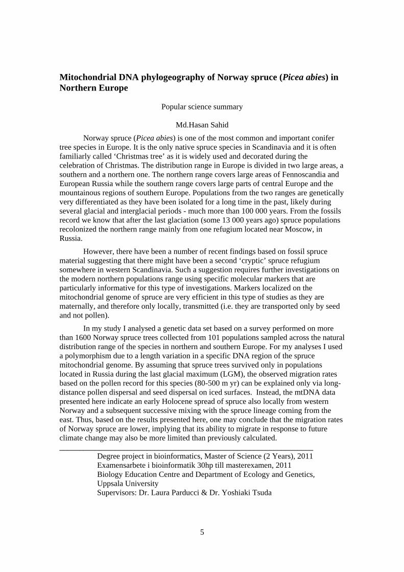
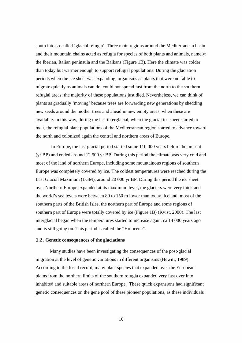
In Europe, most of the mountain regions are located in the southern areas and in general

they are running in an east-west direction (Figure 1A).

Figure 1

(A) Map showing the physical landscape of Europe with mountains in the south running in an east-west direction. Black areas indicate regions over 2000m while dashed line indicates regions over 1000m of altitude. (B) Map showing the picture of the landscape of Europe during the last glacial and hatched symbol represented ice cover at the time of last ice age (Modified from Hewitt, 1999).

During the cold periods of the Pleistocene, the organisms generally living in the

cold regions of northern Europe were dying or, if they were able, they migrated to the

A B

10

south into so-called ‘glacial refugia’. Three main regions around the Mediterranean basin

and their mountain chains acted as refugia for species of both plants and animals, namely:

the Iberian, Italian peninsula and the Balkans (Figure 1B). Here the climate was colder

than today but warmer enough to support refugial populations. During the glaciation

periods when the ice sheet was expanding, organisms as plants that were not able to

migrate quickly as animals can do, could not spread fast from the north to the southern

refugial areas; the majority of these populations just died. Nevertheless, we can think of

plants as gradually ‘moving’ because trees are forwarding new generations by shedding

new seeds around the mother trees and ahead in new empty areas, when these are

available. In this way, during the last interglacial, when the glacial ice sheet started to

melt, the refugial plant populations of the Mediterranean region started to advance toward

the north and colonized again the central and northern areas of Europe.

In Europe, the last glacial period started some 110 000 years before the present

(yr BP) and ended around 12 500 yr BP. During this period the climate was very cold and

most of the land of northern Europe, including some mountainous regions of southern

Europe was completely covered by ice. The coldest temperatures were reached during the

Last Glacial Maximum (LGM), around 20 000 yr BP. During this period the ice sheet

over Northern Europe expanded at its maximum level, the glaciers were very thick and

the world’s sea levels were between 80 to 150 m lower than today. Iceland, most of the

southern parts of the British Isles, the northern part of Europe and some regions of

southern part of Europe were totally covered by ice (Figure 1B) (Kvist, 2000). The last

interglacial began when the temperatures started to increase again, ca 14 000 years ago

and is still going on. This period is called the “Holocene”.

1.2. Genetic consequences of the glaciations

Many studies have been investigating the consequences of the post-glacial

migration at the level of genetic variations in different organisms (Hewitt, 1989).

According to the fossil record, many plant species that expanded over the European

plains from the northern limits of the southern refugia expanded very fast over into

inhabited and suitable areas of northern Europe. These quick expansions had significant

genetic consequences on the gene pool of these pioneer populations, as these individuals

11

dominated with their genes in the following generations. These long distance dispersal

events were repeated several times during the time the species moved towards the north

and these repeated founder events inevitably led to a decrease in the number of alleles

and increased heterozygosity in the central and northern areas of Europe (Hewitt, 1999).

All these events predict that populations in the northern ranges will have their

genetic diversity diminished compared to the southern refugial ones. This will predict

also that the populations that are behind the northern limits of the southern refugia will

not be able to move freely toward the north in pre-occupied areas, and that therefore

higher genetic diversity will be maintained in such regions (Hewitt, 1999). The refugial

populations from the south would need to move to higher latitudes over the available

mountains of the southern areas to survive (Hewitt, 1993a, 1996). The East-West

direction of mountains in Europe in such cases may also have played as a barrier to

distribution expansion, isolating the populations in the southern Mediterranean regions, in

the Iberian Peninsula, Italy, the Balkans and Greece (Figure 1B). Many southern refugial

populations therefore, remained isolated without exchanging genes. When they

eventually start slowly ‘moving’ towards the north they would likely meet in what is now

called ‘admixture’ zones.

However, how did individual species respond to climate changes during glacial

and interglacial periods, depend on their ability to adapt to changing climates and/or to

disperse? The mechanisms related to southern refugia presented above are applied mainly

to temperate forest tree species such as oak and beech. On the other hand, there is now

increasing evidence suggesting ‘cryptic’ refugia for more cold tolerant species such as

spruce and birch in more Northerly area than we previously believed. The concept of

cryptic refugia was conceived for the first time by Stewart and Lister (2001) and it was

applied to organisms that were living in central or northern Europe during the last

glaciation. Such refugia have shown to be very different in size as well and they showed

variation in the duration during which species were confined to them (Stewart et al.,

2009). The presence of such refugia had important implications for the evolution of all

plant species.

12

1.3. The fossil pollen record

Pollen is the male gamete of plants and is haploid. During fertilization pollen

transfers its haploid nuclear genome to the ovule of a plant. However, depending on the

species and the corresponding type of inheritance, it transfers also two additional haploid

genomes: the chloroplast and the mitochondrial genome. Usually pollen is dispersed by

wind and insects, but in the conifers, including Norway spruce, pollen is transported

mainly by wind (Vidakovic, 1991). The pollen grains dispersed in the air during the

reproductive season and that fail to find the female organs, eventually will fall to the

ground. With time, soil layers accumulate and pollen becomes buried into sediments and

eventually also gets partially fossilized.

In paleoecological studies, fossil pollen data obtained from different sites,

particularly from lake sediments, is used to verify the presence of a certain taxon in a

region, to represent its distribution range over time and to show the different migration

routes followed after glacial periods. Samples in the form of sediment cores are usually

extracted from peats or from the bottom of lakes or river basins and are analysed for

pollen content. Particularly in lake sediments the precipitate is very soft which preserves

the pollen better. By using radiocarbon methodology it is possible to accurately date

fossil remains like macrofossils present in such sediments and thus to date the whole

record.

The fossil pollen record is therefore an important tool to study the past history of

plant species. In the last decades, the pollen records of many plant species have identified

several southern Mediterranean regions as the major refugial areas in Europe, clearly

indicating that during the glacial period’s populations mainly survived in these isolated

areas.

1.4. The studied species: Norway spruce (Picea abies L. Karst.)

Norway spruce (Picea abies L. Karst.) is one of the main economically important

forest tree species of northern Europe. It is the only native spruce species in Scandinavia

and it is often familiarly called ‘Christmas tree’ as it is widely used and decorated during

the celebration of Christmas. It is also used for medical purposes, production of timber

13

etc. It is a cold tolerant species but it can adjust easily to different climate conditions. It

grows well in full sunny light areas as well as in cool temperate and wet land regions

(Giesecke and Bennett, 2004). In northern Europe its range covers large parts of the

mountain regions from the Ural Mountains in the east to Norway in the west. The height

of an adult spruce tree can vary between 12 and 20 meters and the width of the trunk may

vary between 1 to 2 meters (Vidakovic, 1991). It is a dark deep green tree with a typical

triangular shape. Spruce is a monoecious species, as the same tree can produce male

(staminate) and female (ovulate) flowers (Tjoelker et al., 2007).

The fossil pollen record tells us that after the last glaciation (from some 13 000 yr

BP) populations of spruce first entered Fennoscandia (the peninsula of Scandinavian, the

Kola peninsula, Karelia and Finland.) from the eastern areas of Europe at different times

and following different routes. Likely, low-density spruce populations first entered

Fenoscandia during the early Holocene (already around 11 000 yr BP) and established in

a few scattered areas of the northern part of Scandinavia. A second main immigration

route with a large population density followed in the middle-late Holocene (5 000 - 3 000

yr BP), in an east to west direction, into the Baltic Republics and Finland.

Accordingly, during the early Holocene in some regions in eastern Finland and

Russia pollen percentage of P. abies reached already 3% of the total pollen sums (values

over 2% in spruce indicate local presence), clearly indicating the presence of large

refugial populations in this area. According to Moe (1970) and Tallantire (1972, 1977)

however, the spread of P. abies in Fennoscandia occurred later, during the mid Holocene

at around 8 000 yr BP. No pollen record from Norway or Sweden shows percentages over

or equal to 2% at this time. However, at around 7 000 yr BP, pollen percentage already

reached 1% in scattered areas of Scandinavia, for example into the Tönningfloarna region

in central Sweden (Giesecke and Bennett, 2004) and at around 6 300 yr BP values over

2% are found in central Norway (Parducci et al., personal communication). In addition

recently, late glacial findings of P. abies macrofossil (pollen and stomata) from central

Norway have provided new additional evidence for the presence of spruce glacial

populations in western Scandinavia already at the beginning of the Holocene (Paus et al.,

2011). Since Norway spruce is a cold tolerant species, its persistence during glacial

periods in northern Europe is reasonable.

14

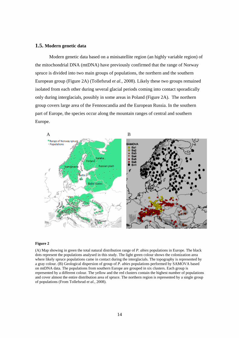
1.5. Modern genetic data

Modern genetic data based on a minisatellite region (an highly variable region) of

the mitochondrial DNA (mtDNA) have previously confirmed that the range of Norway

spruce is divided into two main groups of populations, the northern and the southern

European group (Figure 2A) (Tollefsrud et al., 2008). Likely these two groups remained

isolated from each other during several glacial periods coming into contact sporadically

only during interglacials, possibly in some areas in Poland (Figure 2A). The northern

group covers large area of the Fennoscandia and the European Russia. In the southern

part of Europe, the species occur along the mountain ranges of central and southern

Europe.

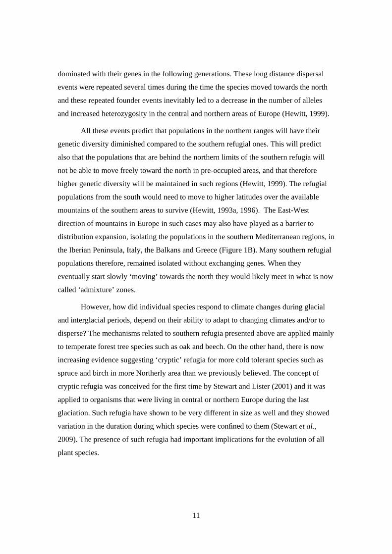
Using SAMOVA (Spatial Analysis of Molecular Variance; Dupanloup et al., ure 2

Figure 2

(A) Map showing in green the total natural distribution range of P. abies populations in Europe. The black dots represent the populations analysed in this study. The light green colour shows the colonization area where likely spruce populations came in contact during the interglacials. The topography is represented by a gray colour. (B) Geological dispersion of group of P. abies populations performed by SAMOVA based on mtDNA data. The populations from southern Europe are grouped in six clusters. Each group is represented by a different colour. The yellow and the red clusters contain the highest number of populations and cover almost the entire distribution area of spruce. The northern region is represented by a single group of populations (From Tollefsrud et al., 2008).

A B

15

Using SAMOVA (Spatial Analysis of Molecular Variance; Dupanloup et al., 2002,

Figure 2B) Tollefsrud et al. (2008) detected a clear spatial population group structure in

northern and southern Europe.

Moreover, they found a two times higher level of genetic differentiation (GST)

among the populations in the southern group (0.479) than in the northern group and

concluded that genetic data was in accordance with the fossil data: one unique refugium

localized in the east around the Moscow region contributed to the main postglacial

recolonization of the northern range of Norway spruce in Europe.

1.6. Aim of this study

Although the northern and southern groups were confirmed by previous analyses,

the genetic structure of the spruce populations from northern Europe was not well

resolved in these previous studies and additional mtDNA information is needed to discuss

the population history of Norway spruce in northern Europe in detail.

The main goal of this work was thus to increase our understanding of the

phylogeography and the postglacial migration history of Norway spruce, in detail, using a

new set of mtDNA data.

2. Materials and methods

2.1. Sample collection and mtDNA variation

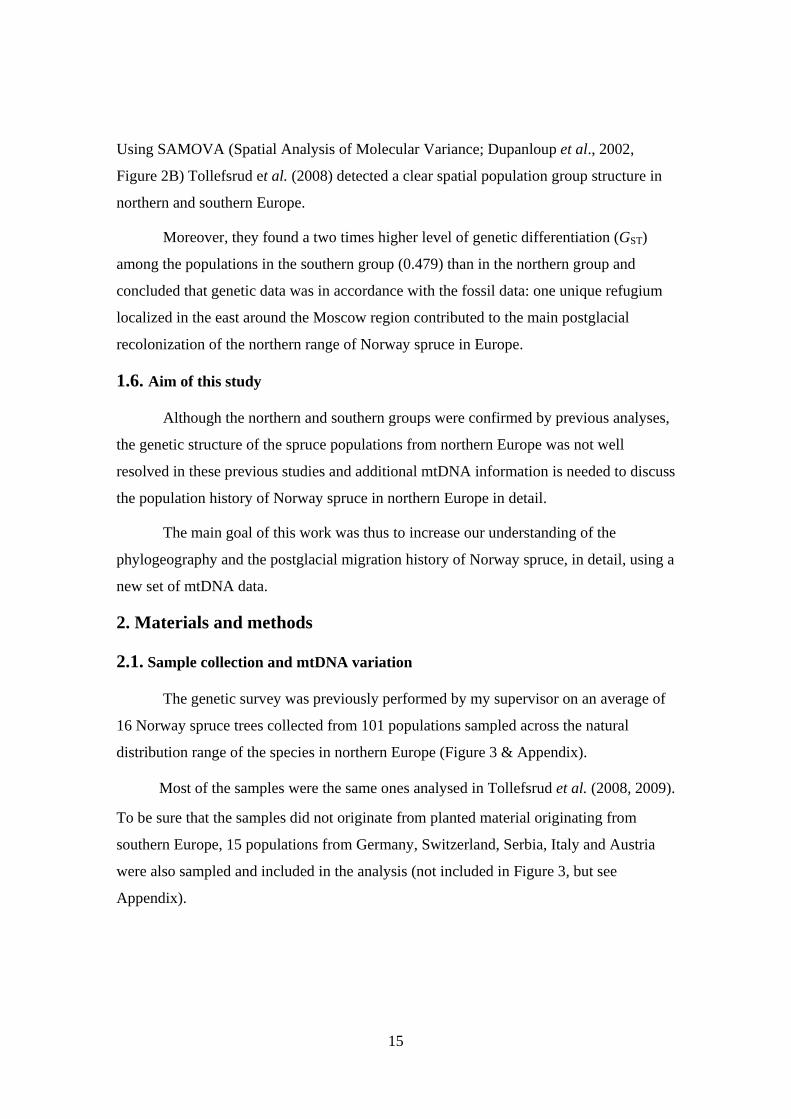
The genetic survey was previously performed by my supervisor on an average of

16 Norway spruce trees collected from 101 populations sampled across the natural

distribution range of the species in northern Europe (Figure 3 & Appendix).

Most of the samples were the same ones analysed in Tollefsrud et al. (2008, 2009).

To be sure that the samples did not originate from planted material originating from

southern Europe, 15 populations from Germany, Switzerland, Serbia, Italy and Austria

were also sampled and included in the analysis (not included in Figure 3, but see

Appendix).

16

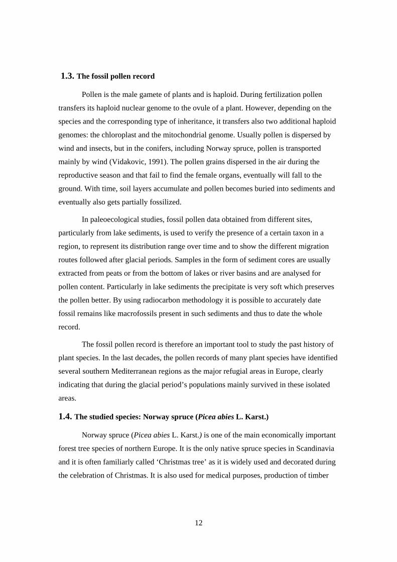
Figure 3

The locations of the 101 Norway spruce populations analysed in this study. Populations are indicated by red circles together with their population codes (detailed information can be found in Appendix). Populations from southern Europe are not included in this map. The map was created using arcGIS based on information from Appendix.

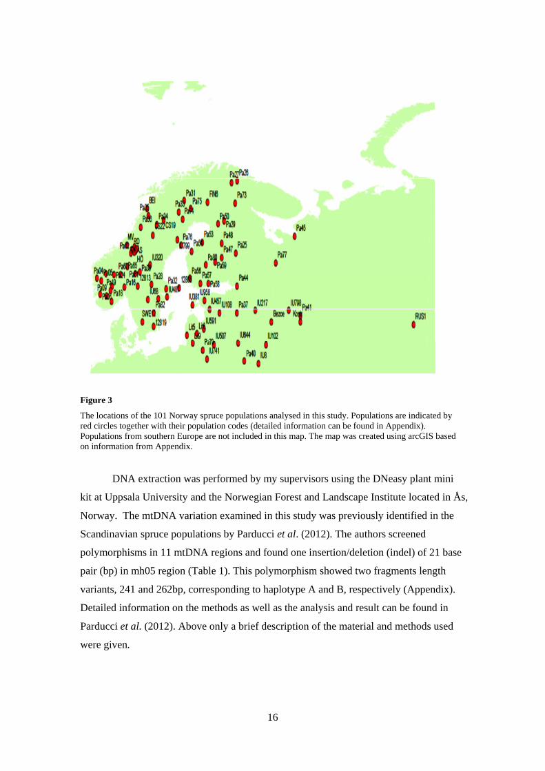
DNA extraction was performed by my supervisors using the DNeasy plant mini

kit at Uppsala University and the Norwegian Forest and Landscape Institute located in Ås,

Norway. The mtDNA variation examined in this study was previously identified in the

Scandinavian spruce populations by Parducci et al. (2012). The authors screened

polymorphisms in 11 mtDNA regions and found one insertion/deletion (indel) of 21 base

pair (bp) in mh05 region (Table 1). This polymorphism showed two fragments length

variants, 241 and 262bp, corresponding to haplotype A and B, respectively (Appendix).

Detailed information on the methods as well as the analysis and result can be found in

Parducci et al. (2012). Above only a brief description of the material and methods used

were given.

17

Table 1

Targeted regions, sequences and approximate product length (bp) of polymerase chain reaction (PCR) for

primer pairs used to amplify 11 mtDNA regions of Norway spruce. Pa; poor amplification.

Region Sequence Length

mh05 5'-GGGAGTCAGCGAAAGAAGTAAG-3' 5'-AGTCTCAGAGCCAGAAGCAG-3' 241-262

mh35 5'-CGATGACATCTCTTAGCTTCC-3' 5'-TGGGGAATAGGATTCGGGTAAG-3' 1000

mh02 5'-TTTTAGGGCCATTTGCCTGC-3' 5'-TCTATGGACAAGAGCCCGACCT-3' 950

mh33' 5'-CGAAGGAAGGAATGAAGGTG-3' 5'-GCTCTTAAGTGCTGGTTGATG-3' 850

mh38 5'-CCGTCCCCTATCCATCAAAC-3' 5'-CCCTGAGCGAGATTGAATTAG-3' 1000

nad5 5'-AGTCCAATAGGGACAGCAC-3' 5'-ACCCGACGATAACTAGCTTC-3' Pa

nad7/1-2 5'-ACCTCAACATCCTGCTGCTC-3' 5'-CGATCAGAATAAGGTAAAGC-3' Pa

mh44 5'-ATGACTGGAAGAATTGCTCAC-3' 5'-TTCACTTGATACTCACCCCC-3' 157

mt15-D02

5'-TATCTGACTTGCCTTATC-3' 5'-ATCCGAATACATACACC-3' 750

mt23D02 5'-CACCCTTGGGTAGACTGG-3' 5'-GGTTCACGCAGTGCTTCT-3' Pa

mt1H01 5'-AAGATGGATCGCCCTTACGC-3' 5'-GAGGAGGAGGCTTCGTCGTC-3' 700

18

2.2. Genetic diversity and differentiation

In this study, I used Excel and manually calculated intrapopulation gene diversity,

average gene diversity, total gene diversity and genetic differentiation among the 101

spruce populations according to Nei (1987).

Gene diversity within population (H)

The gene diversity of a single locus is defined as:

2

1

1

q

i

iPH ------------------------------------------------------------------------------------ (1)

In equation (1) Pi is the population frequency of the i-th allele and q is the total

number of alleles. In a haploid data set, as used in this study, this value means a

possibility that two individuals have different haplotypes when two individuals are

sampled randomly in a population. The range of gene diversity varies between 0 and 1

and higher values mean higher genetic diversity.

Average gene diversity (HS)

The average gene diversity within subpopulations is defined as:

s

k

q

i

kik XWHs 21 ------------------------------------------------------------------------------ (2)

In equation (2) Wk refers to the size of the k-th subpopulations and Xki is the

frequency of the i-th allele in the k-th subpopulation. In other words, this indicator is the

mean value of intra-population gene diversity.

Total gene diversity (HT)

The gene diversity for the total populations can be defined as:

---------------------------------------------------------------------------------- (3)

In equation (3) kiX is the average value of the Xki and Xki is the frequency of the i-

th allele in the k-th subpopulation. This indicator is as same as the gene diversity when all

individuals are pooled into one population.

2

1 q

i ki T X H

19

Genetic differentiation (GST)

Genetic differentiation among the populations is defined as:

T

STST

H

HHG

)( ----------------------------------------------------------------------------------- (4)

In equation (4) HT is the sum of the overall subpopulations and HS refers to the

sum of subpopulations respectively. GST is the value for the genetic differentiation among

the population.

The range of the GST value varies between 0 and 1. If GST is 0, it means that

populations are genetically identical, so there is no genetic differentiation between them.

On the opposite, if GST is equal to 1, then the populations are completely different and

they do not share any allele (Nei, 1987).

3. Results

3.1. Haplotype distribution and genetic structure

The geographical distribution of haplotypes A and B showed a clear genetic

structure over the examined northern range. Haplotype A was restricted to Scandinavia,

whereas haplotype B was found all over the eastern-northern and southern ranges (Figure

3). Twenty-nine out of 101 populations showed intrapopulation genetic variation

(Appendix and Figure 3) and in particular seven populations (Pa 67, Pa 61, Rd, 12813, Pa

34, Pa 36, and MV; Appendix) showed higher gene diversity values. The value of

averaged intrapopulation gene diversity (HS=0.09) was lower than total populations gene

diversity (HT=0.28) and a relatively high value of genetic differentiation was detected

among populations (GST=0.68).

20

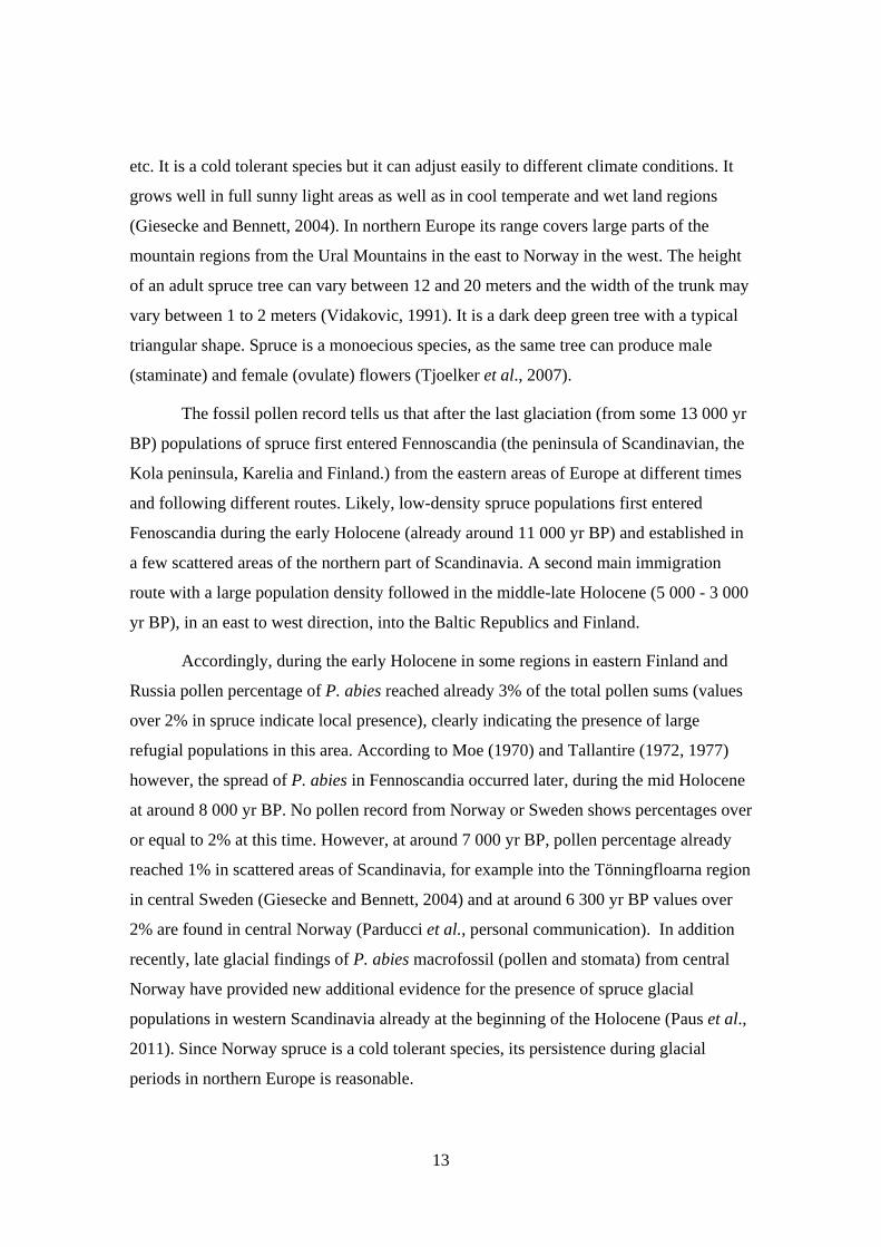
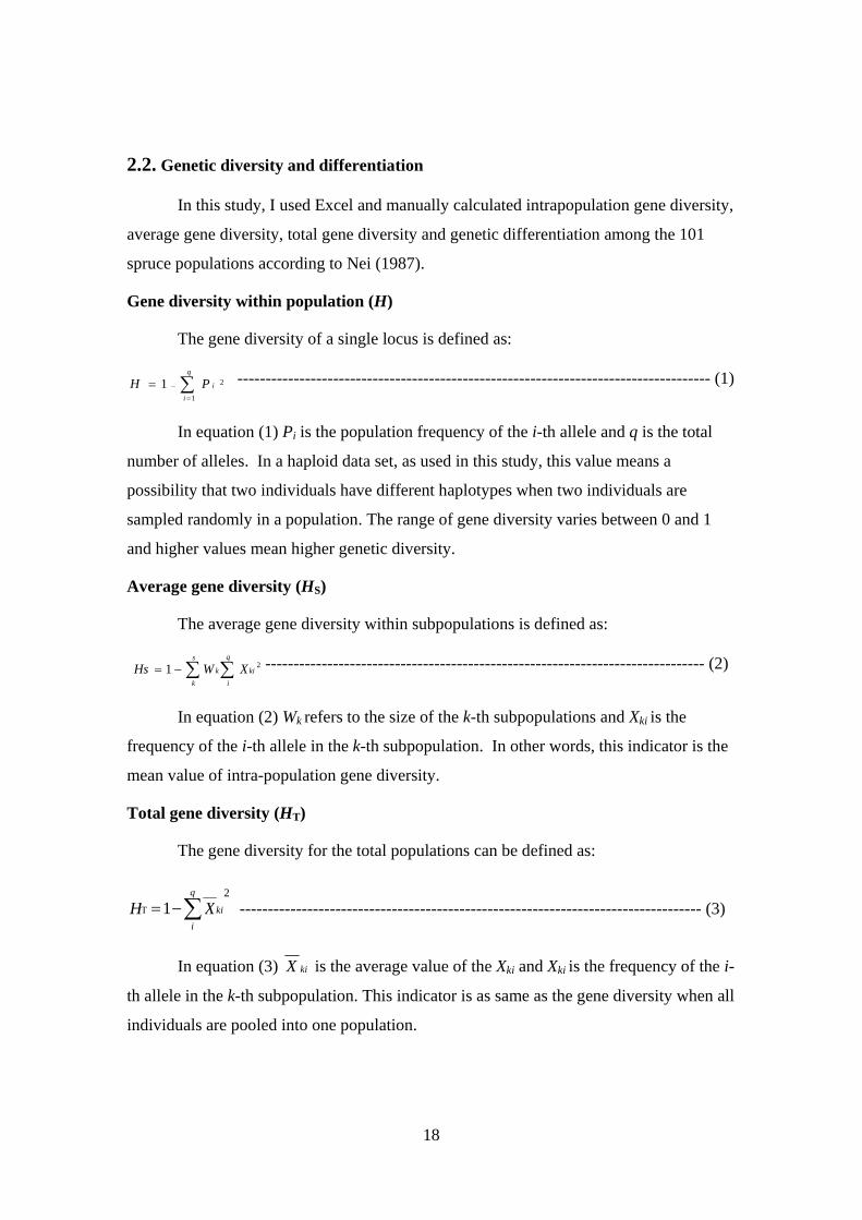
Figure 4

Map showing the modern P. abies populations. The grey shading represents the natural range divided in two main groups: southern and northern. Circles indicate the populations analysed at the mitochondrial polymorphic locus and size of the circles is proportional to population size. The proportion of the Scandinavian haplotype A in each population is shown in black. The highest frequency haplotype A was found in two populations above 67° latitude on the Atlantic coast of Norway. Dark and light blue arrows suggest postglacial movements of the two haplotypes after the LGM based on this data.

4. Discussion

4.1. Comparison of genetic diversity and differentiation with other spruce species

The average gene diversity found in the mtDNA of Norway spruce was very low

(HS=0.09) but similar to the values detected in the mtDNA variation of other conifer

species (e.g. Picea jezoensis, 0.073, Aizawa et al., 2007; Picea asperata, 0.06, Du et al.,

2009).

The genetic diversity among populations was high (GST=0.68) and only slightly

lower than other spruce species based on the same type of markers (Picea jezoensis, 0.90,

Aizawa et al., 2007; Picea asperata, 0.90, Du et al., 2009). In P. abies, GST values in bi-

parentally inherited nuclear DNA (GST = 0.08; Tollefsrud, et al., 2009) and in paternal

inherited chloroplast (cp) DNA (GST =0.099; Vendramin et al., 2000) were much lower

than the value detected in mtDNA in this study. Since the mitochondrial genome is

maternally inherited in spruce (Grivet et al., 1999), gene flow occurs only via seed

21

among populations. Therefore the mtDNA haplotypes were only locally distributed via

seeds and not via pollen as for cp and nuclear DNA markers. In addition, since in plants

the mutation rate of mtDNA is lower than that for nuclear DNA and generally mtDNA

variation is not affected by recombination (Wolfe et al., 1987), mtDNA variation is

expected to show lower intra-population genetic diversity and higher genetic

differentiation among populations than the nuclear one (Petit et al., 1993). The results

detected in this study were in accordance with this expectation.

4.2. Postglacial migration routes of Norway spruce

The geographical distribution of the haplotypes in this study was very structured.

The haplotype A was observed in 29 spruce populations all restricted to Scandinavia.

Especially, the highest frequencies of haplotype A were detected in nine populations in

the western areas of Scandinavia. Considering the low mutation rate and the low ability

of gene flow of mt genomes, this locally structured distribution of haplotype A suggest

that there was another refugium of Norway spruce in Scandinavia; likely in some ice-free

regions on the coast of Norway as here we found the highest frequency of haplotype A.

Likely, haplotype B is the ancestral one as it was found in all the rest of the populations

(i.e. it was the most common one). If haplotype A had been due to a mutation that

occurred during the Holocene in the populations moving from the eastern refugium in

Russia, detection of haplotype A would be expected to occur also along the postglacial

migration route from east to west through Russia. However, these regions in Russia were

completely fixed for the haplotype B. Therefore a likely explanation may be that the

mutation predates the last glaciation and that it occurred in populations that survived in

some ice-free regions on the coast of Norway. This suggestion is also supported by the

fact that haplotype A has recently been detected also in ancient Norway spruce material

(pollen and soils sediments) dated up 10 300 yr BP and collected from lake sediments

retrieved in central Norway (Parducci et al., 2012). 

These results have important implications for the calculation of postglacial

migration rates for spruce. By assuming that spruce trees survived only in populations

located in Russia during the LGM, the observed migration rates based on the pollen

record for this species (80-500 m yr; Huntley et al., 1983) can be explained only via long-

22

distance pollen dispersal and seed dispersal on iced surfaces. Instead, the mtDNA data

presented here indicate an early Holocene spread of spruce also locally from western

Norway and a subsequent successive mixing with the spruce lineage coming from the

east. Thus, based on the results presented here, one may conclude that the migration rates

of Norway spruce are lower, implying that its ability to migrate in response to future

climate change may be more limited than previously calculated. This hypothesis is also in

accordance with recent finding from North America showing that post-glacial migration

speed of tree species is much slower than we previously believed (McLachlan et al.,

2005).

5. Future work

In this study, evidence of past persistence of Norway spruce in Central

Scandinavia during LGM was detected. To evaluate this Northern survival hypothesis,

one would need to test this statistically in future work. It is now possible to use a

sophisticated software, SPLATCHE (Spatial And Temporal Coalescences in

Heterogeneous Environment, Ray et al., 2010) to simulate historical demographic events

that may have caused changes over time in the genetic structure of a large number of

populations and compare this results for likelihood with real observed genetic data.

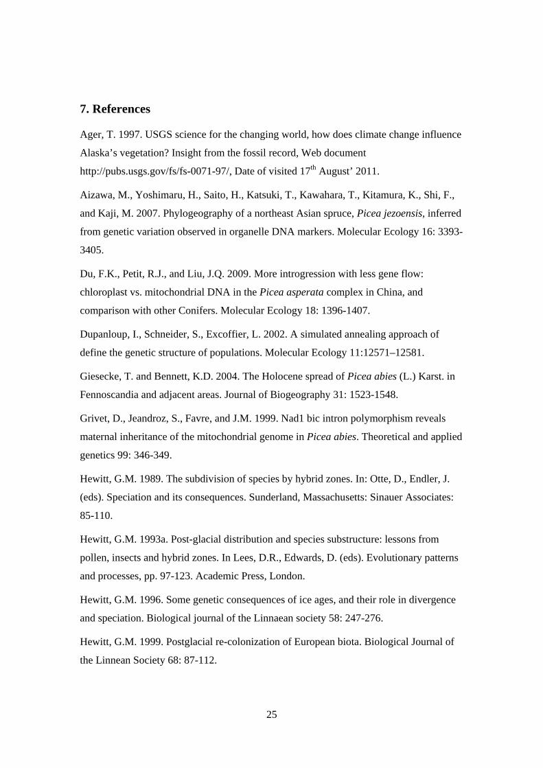
SPLATCHE runs first a forward demographic simulation over a changing environment

over time and successively runs a backward coalescence-based simulation of the genetic

mutations occurring in the populations over the simulated changing environment (Ray et

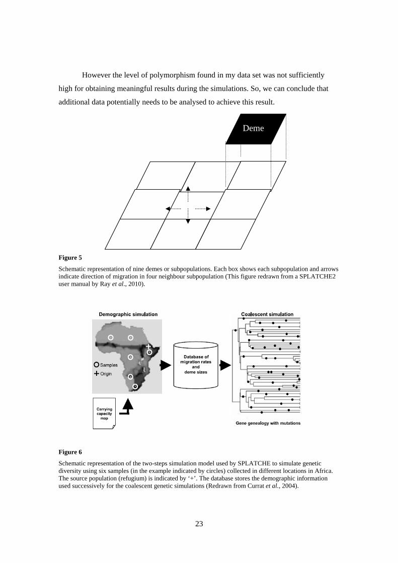
al., 2010). For the demographic simulations the surface of the landscape is divided into a

lattice composed of many subpopulations (or demes). Each subpopulation occupies a

region of 95x73 demes, as shown in (Figure 4). The demographic simulations and

migration history of the populations are stored in a database and are then successively

used for running the second simulation using the coalescence theory. In the end it is

possible to obtain simulated gene genealogies on the different environments with the

occurrence of mutations (Figure 5). Eventually we will compare the real genotypic

mtDNA data with simulated data. I initially attempted to use SPLATCHE to test the two-

refugia hypotheses for Norway spruce using the mtDNA polymorphism described in my

work.

23

However the level of polymorphism found in my data set was not sufficiently

high for obtaining meaningful results during the simulations. So, we can conclude that

additional data potentially needs to be analysed to achieve this result.

Figure 5

Schematic representation of nine demes or subpopulations. Each box shows each subpopulation and arrows indicate direction of migration in four neighbour subpopulation (This figure redrawn from a SPLATCHE2 user manual by Ray et al., 2010).

Figure 6

Schematic representation of the two-steps simulation model used by SPLATCHE to simulate genetic diversity using six samples (in the example indicated by circles) collected in different locations in Africa. The source population (refugium) is indicated by ‘+’. The database stores the demographic information used successively for the coalescent genetic simulations (Redrawn from Currat et al., 2004).

Deme

24

6. Acknowledgements

Firstly, I would like to thank my supervisors, Dr. Laura Parducci and Dr.

Yoshiaki Tsuda for all those instances where they encouraged and helped me throughout

my work. They were kind enough to inform me on the procedures required for

completing a degree project, and explain all the methodologies of my work.

I would also like to thank some other people working in the department: Per

Sjödin, Anna Palmé, and Anders Larsson, who all at many crucial moments when I

needed their guidance, gave me their honest and forthcoming responses which assisted

me to successfully complete my work.

Finally, I would like to thank my family members, who encouraged and supported

me during my education and my studies in Uppsala. I also want to acknowledge my

brother and sisters, because without their love, inspiration, and support I would not have

completed this work.

I dedicate this thesis work to my parents.

25

7. References

Ager, T. 1997. USGS science for the changing world, how does climate change influence

Alaska’s vegetation? Insight from the fossil record, Web document

http://pubs.usgs.gov/fs/fs-0071-97/, Date of visited 17th August’ 2011.

Aizawa, M., Yoshimaru, H., Saito, H., Katsuki, T., Kawahara, T., Kitamura, K., Shi, F.,

and Kaji, M. 2007. Phylogeography of a northeast Asian spruce, Picea jezoensis, inferred

from genetic variation observed in organelle DNA markers. Molecular Ecology 16: 3393-

3405.

Du, F.K., Petit, R.J., and Liu, J.Q. 2009. More introgression with less gene flow:

chloroplast vs. mitochondrial DNA in the Picea asperata complex in China, and

comparison with other Conifers. Molecular Ecology 18: 1396-1407.

Dupanloup, I., Schneider, S., Excoffier, L. 2002. A simulated annealing approach of

define the genetic structure of populations. Molecular Ecology 11:12571–12581.

Giesecke, T. and Bennett, K.D. 2004. The Holocene spread of Picea abies (L.) Karst. in

Fennoscandia and adjacent areas. Journal of Biogeography 31: 1523-1548.

Grivet, D., Jeandroz, S., Favre, and J.M. 1999. Nad1 bic intron polymorphism reveals

maternal inheritance of the mitochondrial genome in Picea abies. Theoretical and applied

genetics 99: 346-349.

Hewitt, G.M. 1989. The subdivision of species by hybrid zones. In: Otte, D., Endler, J.

(eds). Speciation and its consequences. Sunderland, Massachusetts: Sinauer Associates:

85-110.

Hewitt, G.M. 1993a. Post-glacial distribution and species substructure: lessons from

pollen, insects and hybrid zones. In Lees, D.R., Edwards, D. (eds). Evolutionary patterns

and processes, pp. 97-123. Academic Press, London.

Hewitt, G.M. 1996. Some genetic consequences of ice ages, and their role in divergence

and speciation. Biological journal of the Linnaean society 58: 247-276.

Hewitt, G.M. 1999. Postglacial re-colonization of European biota. Biological Journal of

the Linnean Society 68: 87-112.

26

Huntley, B. and Birks, H. J. B. 1983. An Atlas of Past and Present Pollen Maps for

Europe 0-13,000 Years Ago. Cambridge: Cambridge University Press.

Kvist, L. 2000. Phylogeny and phylogeography of European parids. Oulu: Oulun

Yliopisto Kirjasto.

McLachlan, J.S., Clark, J.S., Manos, P.S. 2005. Molecular indicators of tree migration

capacity under rapid climate change. Ecology 86: 2088-2098.

Moe, D. 1970. The post-glacial immigration of Picea abies into Fennosandia. Botaniska

Notiser, 123: 61-66.

Nei, M. 1987. Molecular Evolutionary Genetics. Columbia University Press: New york,

USA.

Parducci, L. 2012. Glacial Survival of Boreal Trees in Northern Scandinavia Revealed by

Modern and Ancient Genetics. Science in press.

Paus, A., Velle, G., and Berge, J. 2011. The lateglacial and early Holocene vegetation

and environment in the Dovre Mountains, central Norway, as signalled in two lateglacial

nunatak lakes. Quaternary Science Reviews 30: 1780-1796.

Petit, R.J., Kremer, A., and Wanger, D.B. 1993. Finite island model for organelle and

nuclear genes in plants. Heredity 71: 630-641.

Pidwirny, M. and Jones, S. 2006. Introduction to the Lithosphere. Fundamental of

Physical Geography. 2nd ed. Web document

http://www.physicalgeography.net/fundamentals/10ad.html, Date of visited 1st July’2011

Ray, N., Currat, M., and Excoffier, L. 2004. SPLATCHE: a program to simulate genetic

diversity taking into account environmental heterogeneity. Molecular Ecology 4: 139-142.

Ray, N., Currat, M., and Excoffier, L., 2010. SPLATCHE 2, Version: 22.09.2010.

http://www.splatche.com/

Stewart, J. and Lister, A.M. 2001. Cryptic northern refugia and the origins of the modern

biota. Trends in Ecology and Evolution 16: 608-613.

Stewart, J.R., Lister, A.M., Barnes, I., and Dalen, L. 2009. Refugia revisited:

individualistic responses of species in space and time. Biological Sciences 277: 661-671.

27

Tallantire, P.A. 1972. The regional spread of spruce (Picea abies (L) Karst.) within

Fennoscandia: a reassessment. Norwegian Journal of Botany 19: 1-16.

Tallantire, P.A. 1977. A further contribution to the problem of the spread of spruce

(Picea abies (L) Karst.). in Fennoscandia. Journal of Biogeography 4: 219-227.

Tjoelker, M.G., Boratynski, A., and Bugala, W. 2007. Biology and ecology of Norway

spruce. 2nd ed. Springer. Dordrecht, Netherlands.

Tollefsrud, M.M., Kissling, R., Gugerli, F., Johnsen, Ø., Skrøppa, T., Cheddadi, R., Van

Der Knaap, W.O., Lataaowa, M., Terhurne-berson, R., Litt, T., Gerburek, T., Brochmann,

C., and Sperisen, C. 2008. Genetic consequences of glacial survival and postglacial

colonization in Norway spruce: combined analysis of mitochondrial DNA and fossil

pollen. Molecular Ecology 17: 4134-4150.

Tollefsrud, M.M., Sønstebø, J.H., Brochmann, C., Johnsen, Ø., Skrøppa, T., and

Vendramin, G.G. 2009. Combined analyses of nuclear and mitochondrial markers

provide new insight into the genetic structure of north European Picea abies. Heredity

102:549-562.

Vendramin, G.G., Anzidei, M., Madaghiele, A., Sperisen, C., and Bucci, G. 2000.

Chloroplast microsatellite analysis reveals the presence of population subdivision in

Norway spruce (Picea abies K.). Genome 43: 68-78.

Vidakovic, M. 1991. Picea abies. In: Brekalo, B., (eds). Conifers, morphology and

variation, pp. 293-328. Grafiekizavod Hrvatske, Croation.

Wolfe, K.H., Li, W.H., and Sharp, P.M. 1987. Rates of nucleotide substitution vary

greatly among plant mitochondrial chloroplast and nuclear DNAs. Evolution 84: 9054-

9058.

28

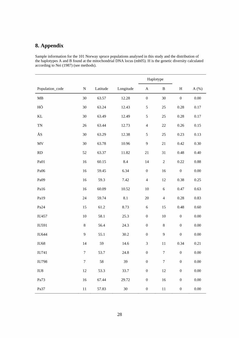
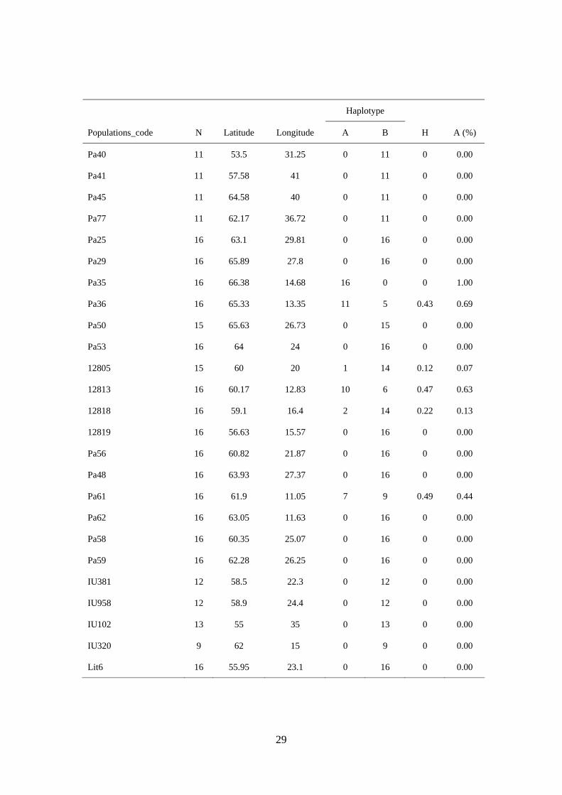
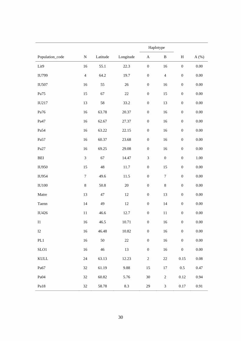
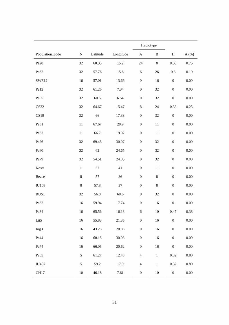
8. Appendix

Sample information for the 101 Norway spruce populations analysed in this study and the distribution of the haplotypes A and B found at the mitochondrial DNA locus (mh05). H is the genetic diversity calculated according to Nei (1987) (see methods).

Haplotype

Population_code N Latitude Longitude A B H A (%)

MB 30 63.57 12.28 0 30 0 0.00

HÖ 30 63.24 12.43 5 25 0.28 0.17

KL 30 63.49 12.49 5 25 0.28 0.17

TN 26 63.44 12.73 4 22 0.26 0.15

ÅS 30 63.29 12.38 5 25 0.23 0.13

MV 30 63.78 10.96 9 21 0.42 0.30

RD 52 63.37 11.82 21 31 0.48 0.40

Pa01 16 60.15 8.4 14 2 0.22 0.88

Pa06 16 59.45 6.34 0 16 0 0.00

Pa09 16 59.3 7.42 4 12 0.38 0.25

Pa16 16 60.09 10.52 10 6 0.47 0.63

Pa19 24 59.74 8.1 20 4 0.28 0.83

Pa24 15 61.2 8.73 6 15 0.48 0.60

IU457 10 58.1 25.3 0 10 0 0.00

IU591 8 56.4 24.3 0 8 0 0.00

IU644 9 55.1 30.2 0 9 0 0.00

IU68 14 59 14.6 3 11 0.34 0.21

IU741 7 53.7 24.8 0 7 0 0.00

IU798 7 58 39 0 7 0 0.00

IU8 12 53.3 33.7 0 12 0 0.00

Pa73 16 67.44 29.72 0 16 0 0.00

Pa37 11 57.83 30 0 11 0 0.00

29

Haplotype

Populations_code N Latitude Longitude A B H A (%)

Pa40 11 53.5 31.25 0 11 0 0.00

Pa41 11 57.58 41 0 11 0 0.00

Pa45 11 64.58 40 0 11 0 0.00

Pa77 11 62.17 36.72 0 11 0 0.00

Pa25 16 63.1 29.81 0 16 0 0.00

Pa29 16 65.89 27.8 0 16 0 0.00

Pa35 16 66.38 14.68 16 0 0 1.00

Pa36 16 65.33 13.35 11 5 0.43 0.69

Pa50 15 65.63 26.73 0 15 0 0.00

Pa53 16 64 24 0 16 0 0.00

12805 15 60 20 1 14 0.12 0.07

12813 16 60.17 12.83 10 6 0.47 0.63

12818 16 59.1 16.4 2 14 0.22 0.13

12819 16 56.63 15.57 0 16 0 0.00

Pa56 16 60.82 21.87 0 16 0 0.00

Pa48 16 63.93 27.37 0 16 0 0.00

Pa61 16 61.9 11.05 7 9 0.49 0.44

Pa62 16 63.05 11.63 0 16 0 0.00

Pa58 16 60.35 25.07 0 16 0 0.00

Pa59 16 62.28 26.25 0 16 0 0.00

IU381 12 58.5 22.3 0 12 0 0.00

IU958 12 58.9 24.4 0 12 0 0.00

IU102 13 55 35 0 13 0 0.00

IU320 9 62 15 0 9 0 0.00

Lit6 16 55.95 23.1 0 16 0 0.00

30

Haplotype

Population_code N Latitude Longitude A B H A (%)

Lit9 16 55.1 22.3 0 16 0 0.00

IU799 4 64.2 19.7 0 4 0 0.00

IU507 16 55 26 0 16 0 0.00

Pa75 15 67 22 0 15 0 0.00

IU217 13 58 33.2 0 13 0 0.00

Pa76 16 63.78 20.37 0 16 0 0.00

Pa47 16 62.67 27.37 0 16 0 0.00

Pa54 16 63.22 22.15 0 16 0 0.00

Pa57 16 60.37 23.68 0 16 0 0.00

Pa27 16 69.25 29.08 0 16 0 0.00

BEI 3 67 14.47 3 0 0 1.00

IU950 15 48 11.7 0 15 0 0.00

IU954 7 49.6 11.5 0 7 0 0.00

IU100 8 50.8 20 0 8 0 0.00

Matre 13 47 12 0 13 0 0.00

Taenn 14 49 12 0 14 0 0.00

IU426 11 46.6 12.7 0 11 0 0.00

I1 16 46.5 10.71 0 16 0 0.00

I2 16 46.48 10.82 0 16 0 0.00

PL1 16 50 22 0 16 0 0.00

SLO1 16 46 13 0 16 0 0.00

KULL 24 63.13 12.23 2 22 0.15 0.08

Pa67 32 61.19 9.88 15 17 0.5 0.47

Pa04 32 60.82 5.76 30 2 0.12 0.94

Pa18 32 58.78 8.3 29 3 0.17 0.91

31

Haplotype

Population_code N Latitude Longitude A B H A (%)

Pa28 32 60.33 15.2 24 8 0.38 0.75

Pa82 32 57.76 15.6 6 26 0.3 0.19

SWE12 16 57.01 13.66 0 16 0 0.00

Pa12 32 61.26 7.34 0 32 0 0.00

Pa05 32 60.6 6.54 0 32 0 0.00

CS22 32 64.67 15.47 8 24 0.38 0.25

CS19 32 66 17.33 0 32 0 0.00

Pa31 11 67.67 20.9 0 11 0 0.00

Pa33 11 66.7 19.92 0 11 0 0.00

Pa26 32 69.45 30.07 0 32 0 0.00

Pa80 32 62 24.65 0 32 0 0.00

Pa79 32 54.51 24.05 0 32 0 0.00

Kostr 11 57 41 0 11 0 0.00

Bezce 8 57 36 0 8 0 0.00

IU108 8 57.8 27 0 8 0 0.00

RUS1 32 56.8 60.6 0 32 0 0.00

Pa32 16 59.94 17.74 0 16 0 0.00

Pa34 16 65.56 16.13 6 10 0.47 0.38

Lit5 16 55.83 21.35 0 16 0 0.00

Jug3 16 43.25 20.83 0 16 0 0.00

Pa44 16 60.18 30.03 0 16 0 0.00

Pa74 16 66.05 20.62 0 16 0 0.00

Pa65 5 61.27 12.43 4 1 0.32 0.80

IU487 5 59.2 17.9 4 1 0.32 0.80

CH17 10 46.18 7.61 0 10 0 0.00

32

Haplotype

Population_code N Latitude Longitude A B H A (%)

FIN6 15 67.53 24.93 0 15 0 0.00

CH20 16 46.23 8.56 0 16 0 0.00

Pa39 15 61.4 13.2 13 2 0.23 0.87

UA1 10 48.12 24.46 0 10 0 0.00