Embed Size (px)
Citation preview

8/4/2014 © CelPlan International, Inc. www.celplan.com 1
MIMO What is real, what is Wishful
Thinking?
Leonhard Korowajczuk CEO/CTO
CelPlan International, Inc. www.celplan.com

8/4/2014 © CelPlan International, Inc. www.celplan.com 2
Presenter • Leonhard Korowajczuk
– CEO/CTO CelPlan International – 45 years of experience in the telecom field (R&D,
manufacturing and service areas) – Holds13 patents – Published books
• “Designing cdma2000 Systems” – published by Wiley in 2006- 963 pages, available in hard
cover, e-book and Kindle
• “LTE , WiMAX and WLAN Network Design, Optimization and Performance Analysis ”
– published by Wiley in June 2011- 750 pages, available in hard cover, e-book and Kindle
– Books in Preparation: • LTE , WiMAX and WLAN Network Design,
Optimization and Performance Analysis – second edition (2014) LTE-A and WiMAX 2.1(1,000+
pages)
• Network Video: Private and Public Safety Applications (2014)
• Backhaul Network Design (2015) • Multi-Technology Networks: from GSM to LTE (2015) • Smart Grids Network Design (2016)
2nd edition

8/4/2014 © CelPlan International, Inc. www.celplan.com 3
CelPlan International • Employee owned enterprise
with international presence – Headquarters in USA – 450 plus employees – Twenty (20) years in business
• Subsidiaries in 6 countries with worldwide operation
• Vendor Independent • Network Design Software
(CelPlanner Suite/CellDesigner)
• Network Design Services • Network Optimization
Services • Network Performance
Evaluation
• Services are provided to equipment vendors, operators and consultants
• High Level Consulting – RFP preparation – Vendor interface – Technical Audit – Business Plan Preparation – Specialized (Smart Grids,
Aeronautical, Windmill, …)
• Network Managed Services • 2G, 3G, 4G, 5G Technologies • Multi-technology / Multi-band
Networks • Backhaul, Small cells, Indoor,
HetNet, Wi-Fi offloading

8/4/2014 © CelPlan International, Inc. www.celplan.com 4
CelPlan Webinar Series • How to Dimension user Traffic in 4 G networks
• May 7th 2014
• How to Consider Overhead in LTE Dimensioning and what is the impact • June 4th 2014
• How to Take into Account Customer Experience when Designing a Wireless Network • July 9th 2014
• LTE Measurements what they mean and how they are used? • August 6th2014
• What LTE parameters need to be Dimensioned and Optimized? Can reuse of one be used? What is the best LTE configuration? • September 3rd 2014/ September 17th, 2014
• Spectrum Analysis for LTE Systems • October 1st 2014
• MIMO: What is real, what is Wishful Thinking? • November 5th 2014
• Send suggestions and questions to: [email protected]

8/4/2014 © CelPlan International, Inc. www.celplan.com 5
Webinar 1 (May 2014) How to Dimension User Traffic in 4G
Networks
Participants from 44 countries Youtube views: 1144

8/4/2014 © CelPlan International, Inc. www.celplan.com 6
User Traffic
1. How to Dimension User Traffic in 4G Networks
2. How to Characterize Data Traffic
3. Data Speed Considerations
4. How to calculate user traffic?
5. Bearers
6. User Applications Determination
7. User Distribution

8/4/2014 © CelPlan International, Inc. www.celplan.com 7
Webinar 2 (June 2014) How to consider overhead in LTE
dimensioning and what is the impact
Participants from 49 countries Youtube views: 545

8/4/2014 © CelPlan International, Inc. www.celplan.com 8
Overhead in LTE 1. Reuse in LTE 2. LTE Refresher
1. Frame 2. Frame Content 3. Transmission Modes 4. Frame Organization
1. Downlink Signals 2. Uplink Signals 3. Downlink Channels 4. Uplink Channels
5. Data Scheduling and Allocation 6. Cellular Reuse
3. Dimensioning and Planning 4. Capacity Calculator

8/4/2014 © CelPlan International, Inc. www.celplan.com 9
Webinar 3 (July 2014) How to consider Customer Experience
when designing a wireless network
Participants from 40 countries Youtube views: 467

8/4/2014 © CelPlan International, Inc. www.celplan.com 10
Customer Experience
1. How to evaluate Customer Experience?
2. What factors affect customer experience?
3. Parameters that affect cutomer experience
4. SINR availability and how to calculate it
5. Conclusions
6. New Products

8/4/2014 © CelPlan International, Inc. www.celplan.com 11
Webinar 4 (August 6th, 2014) LTE Measurements What they mean?
How are they used?
Participants from 44 countries Youtube views: 686
8/4/2014 © CelPlan International, Inc. www.celplan.com 12
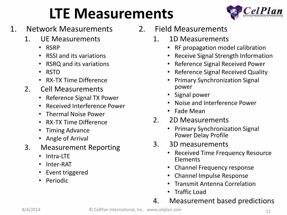
LTE Measurements 1. Network Measurements
1. UE Measurements • RSRP • RSSI and its variations • RSRQ and its variations • RSTD • RX-TX Time Difference
2. Cell Measurements • Reference Signal TX Power • Received Interference Power • Thermal Noise Power • RX-TX Time Difference • Timing Advance • Angle of Arrival
3. Measurement Reporting • Intra-LTE • Inter-RAT • Event triggered • Periodic
2. Field Measurements 1. 1D Measurements
• RF propagation model calibration • Receive Signal Strength Information • Reference Signal Received Power • Reference Signal Received Quality • Primary Synchronization Signal
power • Signal power • Noise and Interference Power • Fade Mean
2. 2D Measurements • Primary Synchronization Signal
Power Delay Profile
3. 3D measurements • Received Time Frequency Resource
Elements • Channel Frequency response • Channel Impulse Response • Transmit Antenna Correlation • Traffic Load
4. Measurement based predictions
8/4/2014 © CelPlan International, Inc. www.celplan.com 13
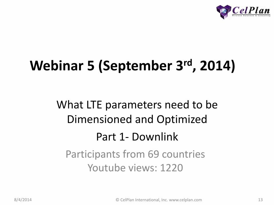
Webinar 5 (September 3rd, 2014)
What LTE parameters need to be Dimensioned and Optimized
Part 1- Downlink
Participants from 69 countries Youtube views: 1220

8/4/2014 © CelPlan International, Inc. www.celplan.com 14
Webinar 5 (September 16th, 2014)
What LTE parameters need to be Dimensioned and Optimized
Part 2- Uplink
Participants from 46 countries Youtube views: 316

8/4/2014 © CelPlan International, Inc. www.celplan.com 15
Webinar 6 Spectrum Analysis for LTE Systems
October 1st 2014
Participants from x countries
Youtube views: 145
8/4/2014 © CelPlan International, Inc. www.celplan.com 16
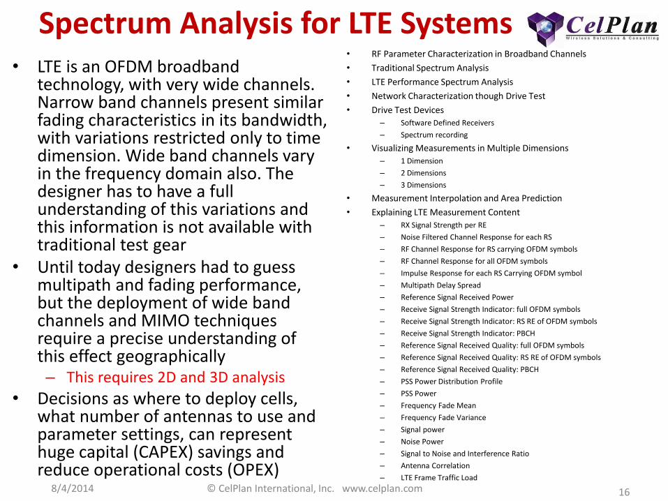
Spectrum Analysis for LTE Systems • LTE is an OFDM broadband
technology, with very wide channels. Narrow band channels present similar fading characteristics in its bandwidth, with variations restricted only to time dimension. Wide band channels vary in the frequency domain also. The designer has to have a full understanding of this variations and this information is not available with traditional test gear
• Until today designers had to guess multipath and fading performance, but the deployment of wide band channels and MIMO techniques require a precise understanding of this effect geographically – This requires 2D and 3D analysis
• Decisions as where to deploy cells, what number of antennas to use and parameter settings, can represent huge capital (CAPEX) savings and reduce operational costs (OPEX)
• RF Parameter Characterization in Broadband Channels
• Traditional Spectrum Analysis
• LTE Performance Spectrum Analysis
• Network Characterization though Drive Test
• Drive Test Devices
– Software Defined Receivers
– Spectrum recording
• Visualizing Measurements in Multiple Dimensions
– 1 Dimension
– 2 Dimensions
– 3 Dimensions
• Measurement Interpolation and Area Prediction
• Explaining LTE Measurement Content
– RX Signal Strength per RE
– Noise Filtered Channel Response for each RS
– RF Channel Response for RS carrying OFDM symbols
– RF Channel Response for all OFDM symbols
– Impulse Response for each RS Carrying OFDM symbol
– Multipath Delay Spread
– Reference Signal Received Power
– Receive Signal Strength Indicator: full OFDM symbols
– Receive Signal Strength Indicator: RS RE of OFDM symbols
– Receive Signal Strength Indicator: PBCH
– Reference Signal Received Quality: full OFDM symbols
– Reference Signal Received Quality: RS RE of OFDM symbols
– Reference Signal Received Quality: PBCH
– PSS Power Distribution Profile
– PSS Power
– Frequency Fade Mean
– Frequency Fade Variance
– Signal power
– Noise Power
– Signal to Noise and Interference Ratio
– Antenna Correlation
– LTE Frame Traffic Load

8/4/2014 © CelPlan International, Inc. www.celplan.com 17
LTE Technology, Network Design & Optimization Boot Camp
December 8 to 12, 2014
at University of West Indies (UWI)
St. Augustine, Trinidad

8/4/2014 © CelPlan International, Inc. www.celplan.com 18
LTE Technology, Network Design & Optimization Boot Camp
• December 8 to 12, 2014
• Based on the current book and updates from the soon-to-be published 2nd edition of, "LTE, WiMAX, and WLAN: Network Design, Optimization and Performance Analysis", by Leonhard Korowajczuk, this -day course presents students with comprehensive information on LTE technology, projects, and deployments.
• CelPlan presents a realistic view of LTE networks, explaining what are just marketing claims and what can be achieved in real life deployments. Each module is taught by experienced 4G RF engineers who design and optimize networks around the globe.
• The materials provided are based upon this experience and by the development of industry leading planning & optimization tools, such as the CelPlanner Software Suite, which is also provided as a 30-day demo to each student
• Module A: LTE Technology – Signal Processing Applied to Wireless Communications
– LTE Technology Overview
– Connecting to an LTE network: an UE point of view
– How to calculate the capacity of an LTE cell and network
– Understanding scheduling algorithms
– LTE measurements and what they mean
– Understanding MIMO: Distinguishing between reality and wishful thinking
– Analyzing 3D RF broadband drive test

8/4/2014 © CelPlan International, Inc. www.celplan.com 19
LTE Technology, Network Design & Optimization Boot Camp
• Module B: LTE Network Design – Modeling the LTE Network
– Building Network Component Libraries
– Modeling user services and traffic
– Creating Traffic Layers
– RF Propagation Models and its calibration
– Signal Level Predictions
– LTE Predictions
– LTE Parameters
– LTE Resource Optimization
– LTE Traffic Simulation
– LTE Performance
– Interactive Workshop (sharing experiences)
• 4G Certification (Optional)
• Additional information, Pricing & Registration available at www.celplan.com

8/4/2014 © CelPlan International, Inc. www.celplan.com 20
Today’s Feature Presentation

8/4/2014 © CelPlan International, Inc. www.celplan.com 21
Webinar 7 MIMO
What is Real? What is Wishful Thinking?
November 5th 2014

8/4/2014 © CelPlan International, Inc. www.celplan.com 22
Content 1. Support Theory 2. Antenna Ports 3. Transmission Modes 4. RF Channel 5. MIMO
1. SISO 2. SIMO 3. MISO 4. MIMO 5. Multi-user MIMO
6. Antenna Correlation 7. AAS 8. MIMO Performance 9. CelPlan New Products

8/4/2014 © CelPlan International, Inc. www.celplan.com 23
1. Support Theory
Mathematics
Signal Processing

8/4/2014 © CelPlan International, Inc. www.celplan.com 24
1.1 Mathematics
Polynomial Decomposition
Exponential Number
Matrixes

8/4/2014 © CelPlan International, Inc. www.celplan.com 25
Polynomial Decomposition • In 1712, Brook Taylor demonstrated that a differentiable function around a given point can be
approximated by a polynomial whose coefficients are the derivatives of the function at that point • The Taylor series is then a representation of a function as an infinite sum of terms calculated from its
derivatives at a single point. If this series is centered at zero it is called a MacLaurin series • A function f(x), differentiable at a point a, can be approximated by the polynomial in equation
𝑓 𝑥 = 𝑓 𝑎 + 𝑓′ 𝑎
1!𝑥 − 𝑎 +
𝑓′′ 𝑎
2!𝑥 − 𝑎 2 +
𝑓(3) 𝑎
3!𝑥 − 𝑎 3 + …… . Approximation of differentiable function f(x)
𝑓 𝑥 = 𝑓 0 + 𝑓′(0)𝑥 + 𝑓′′ 0
2!𝑥2 + 𝑓(3) 0
3!𝑥3 + …… . MacLaurin series
𝑠𝑖𝑛′ 𝑥 = 𝑐𝑜𝑠 (𝑥) Differentiation of sin (x)
𝑐𝑜𝑠′(𝑥) = −𝑠𝑖𝑛 (𝑥) Differentiation of cos (x)
𝑠𝑖𝑛 0 = 0 Sin of 0
𝑐𝑜𝑠 0 = 1 Cos of 0
𝑐𝑜𝑠 𝜃 = 1 −𝜃2
2!+𝜃4
4!−𝜃6
6! Cosine decomposition
sin 𝜃 = 𝜃 −𝜃3
3!+𝜃5
5!−𝜃7
7! Sine decomposition

8/4/2014 © CelPlan International, Inc. www.celplan.com 26
Exponential Number (e)
• The power function 𝑓 𝑥 = 𝑎𝑥 is very useful to represent variations that are experienced in real life and its representation by polynomials has been sought
• When we apply Taylor’s expansion to the exponential function we have to calculate its derivative at a point, which is given by equation
𝑓′ 𝑥0 = lim[ 𝑓 𝑥0 + δ − 𝑓 𝑥0 /δ] Function derivative at a point when δ→0
𝑓 ′ 𝑎𝑥0 = 𝑙𝑖𝑚[(𝑎δ−1)/δ] Derivative of 𝑎𝑥0 when δ→0
• Calculating the above limit when δ→0, we see that it is less than 1 for a =2 and greater than 1 for a=3. It is possible then to find a value of a, for which this limit is equal to 1 and the derivative of the function will then be itself. This value is irrational and is approximated by 2.718281….
• This mathematical constant is a unique real number with its derivative at a point x=0 exactly equal to itself. This number is called the exponential number and is represented by “e”.
• The MacLaurin expansion of 𝑒𝑖𝜃is given by
𝑒𝑖𝜃 = 1 + 𝑖θ −𝜃2
2!−𝑖𝜃3
3!+𝜃4
4!+𝑖𝜃5
5!−𝜃6
6!−𝑖𝜃7
7!+ ⋯ MacLaurin expansion of 𝑒𝑖𝜃
𝑅𝑒 𝑒𝑖θ = 1 −𝜃2
2!+𝜃4
4!−𝜃6
6!+ ⋯ Real part of 𝑒𝑖θ
𝐼𝑚 𝑒𝑖θ = θ −𝜃3
3!+𝜃5
5!−𝜃7
7!+ ⋯ Imaginary part of 𝑒𝑖θ
𝑒𝑖θ = 𝑐𝑜𝑠 𝜃 + 𝑖 𝑠𝑖𝑛(𝜃) Euler’s formula 𝑒𝑖θ as a function f sin and cos
eiθ
real numbers
imaginary numbers
complex
plane
+1-1
+i
-i

8/4/2014 © CelPlan International, Inc. www.celplan.com 27
Matrices
8/4/2014 © CelPlan International, Inc. www.celplan.com 28
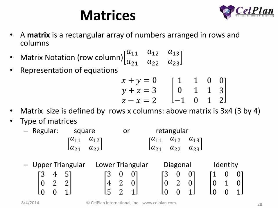
Matrices • A matrix is a rectangular array of numbers arranged in rows and
columns
• Matrix Notation (row column)𝑎11 𝑎12 𝑎13𝑎21 𝑎22 𝑎23
• Representation of equations 𝑥 + 𝑦 = 0 𝑦 + 𝑧 = 3 𝑧 − 𝑥 = 2
• Matrix size is defined by rows x columns: above matrix is 3x4 (3 by 4) • Type of matrices
– Regular: square or retangular
𝑎11 𝑎12𝑎21 𝑎22
𝑎11 𝑎12 𝑎13𝑎21 𝑎22 𝑎23
– Upper Triangular Lower Triangular Diagonal Identity
3 4 50 2 20 0 1
3 0 04 2 05 2 1
3 0 00 2 00 0 1
1 0 00 1 00 0 1

8/4/2014 © CelPlan International, Inc. www.celplan.com 29
Matrix Operations
• Addition: 0 19 8+6 53 4=6 612 12
– Matrices must have same size
• Subtraction: 0 19 8−6 53 4=−6 −46 4
• Matrices must have same size
• Scalar Product: 2 ∗ 0 19 8=0 218 16
8/4/2014 © CelPlan International, Inc. www.celplan.com 30
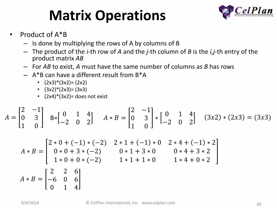
Matrix Operations • Product of A*B
– Is done by multiplying the rows of A by columns of B – The product of the i-th row of A and the j-th column of B is the i,j-th entry of the
product matrix AB – For AB to exist, A must have the same number of columns as B has rows – A*B can have a different result from B*A
• (2x3)*(3x2)= (2x2) • (3x2)*(2x3)= (3x3) • (2x4)*(3x2)= does not exist
𝐴 =2 −10 31 0
B=0 1 4−2 0 2
𝐴 ∗ 𝐵 =2 −10 31 0
∗0 1 4−2 0 2
3𝑥2 ∗ 2𝑥3 = (3𝑥3)
𝐴 ∗ 𝐵 =
2 ∗ 0 + (−1) ∗ (−2) 2 ∗ 1 + −1 ∗ 0 2 ∗ 4 + −1 ∗ 20 ∗ 0 + 3 ∗ (−2) 0 ∗ 1 + 3 ∗ 0 0 ∗ 4 + 3 ∗ 21 ∗ 0 + 0 ∗ (−2) 1 ∗ 1 + 1 ∗ 0 1 ∗ 4 + 0 ∗ 2
𝐴 ∗ 𝐵 =2 2 6−6 0 60 1 4
8/4/2014 © CelPlan International, Inc. www.celplan.com 31
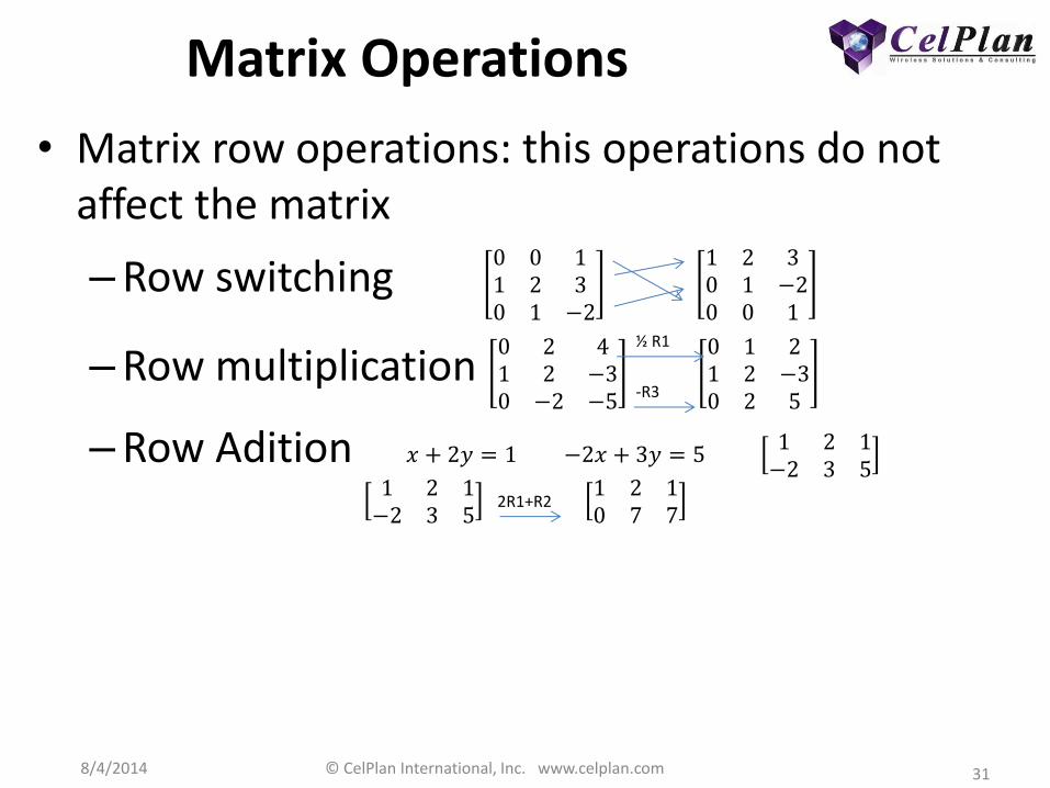
Matrix Operations
• Matrix row operations: this operations do not affect the matrix
–Row switching 0 0 11 2 30 1 −2
1 2 30 1 −20 0 1
–Row multiplication 0 2 41 2 −30 −2 −5
0 1 21 2 −30 2 5
–Row Adition 𝑥 + 2𝑦 = 1 −2𝑥 + 3𝑦 = 5 1 2 1−2 3 5
1 2 1−2 3 5
1 2 10 7 7
½ R1
-R3
2R1+R2

8/4/2014 © CelPlan International, Inc. www.celplan.com 32
Matrix Reduction • Echelon form of a matrix
– A matrix is in row echelon form (ref) when it satisfies the following conditions • The first non-zero element in each row, called
the leading entry, is 1 • Each leading entry is in a column to the right
of the leading entry in the previous row • Rows with all zero elements, if any, are below
rows having a non-zero element
• A matrix is in reduced row echelon form (rref) when it satisfies the following conditions. – The matrix satisfies conditions for a row
echelon form – The leading entry in each row is the only
non-zero entry in its column
1 2 30 0 10 0 0
1 20 10 0
1 2 00 0 10 0 0
1 00 10 0

8/4/2014 © CelPlan International, Inc. www.celplan.com 33
Matrix Rank
• Matrix Rank – The rank of a matrix is defined as
• The maximum number of linearly independent column vectors in the matrix or
• The maximum number of linearly independent row vectors in the matrix. Both definitions are equivalent. For an r x c matrix:
– If r is less than c, then the maximum rank of the matrix is r
– If r is greater than c, then the maximum rank of the matrix is c
– The maximum number of linearly independent vectors in a matrix is equal to the number of non-zero rows in its row echelon matrix • Therefore, to find the rank of a matrix, we simply transform the
matrix to its row echelon form and count the number of non-zero rows
8/4/2014 © CelPlan International, Inc. www.celplan.com 34
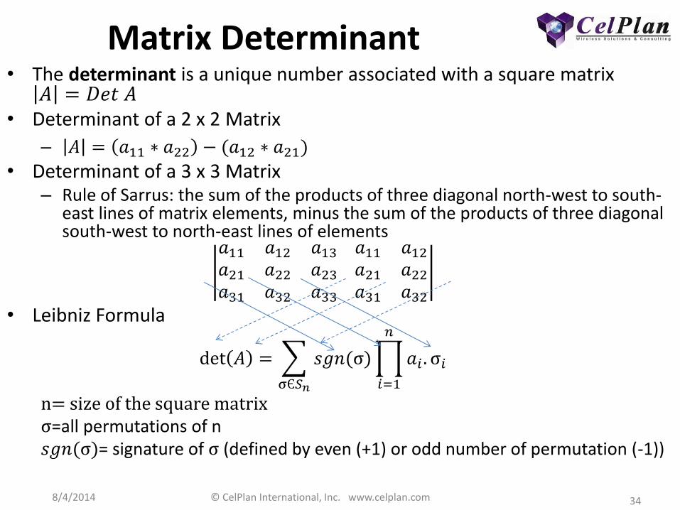
Matrix Determinant • The determinant is a unique number associated with a square matrix 𝐴 = 𝐷𝑒𝑡 𝐴
• Determinant of a 2 x 2 Matrix
– 𝐴 = 𝑎11 ∗ 𝑎22 − (𝑎12 ∗ 𝑎21)
• Determinant of a 3 x 3 Matrix – Rule of Sarrus: the sum of the products of three diagonal north-west to south-
east lines of matrix elements, minus the sum of the products of three diagonal south-west to north-east lines of elements
𝑎11 𝑎12 𝑎13𝑎21 𝑎22 𝑎23𝑎31 𝑎32 𝑎33
𝑎11 𝑎12𝑎21 𝑎22𝑎31 𝑎32
• Leibniz Formula
det 𝐴 = 𝑠𝑔𝑛(σ) 𝑎𝑖 . σ𝑖
𝑛
𝑖=1σЄ𝑆𝑛
n= size of the square matrix σ=all permutations of n 𝑠𝑔𝑛(σ)= signature of σ (defined by even (+1) or odd number of permutation (-1))

8/4/2014 © CelPlan International, Inc. www.celplan.com 35
Matrix Inversion
• The inverse of matrix A is another n x n matrix, denoted A-1, that satisfies the following condition:
𝐴𝐴−1 = 𝐴−1𝐴 = 𝐼𝑛 𝐼𝑛= identity matrix
• Matrix inversion – There is no matrix division, but there is the concept of
matrix inversion – The rank of a matrix is a unique number associated with a
square matrix • If the rank of an n x n matrix is less than n, the matrix does not
have an inverse
– The determinant is another unique number associated with a square matrix • When the determinant for a square matrix is equal to zero, the
inverse for that matrix does not exist

8/4/2014 © CelPlan International, Inc. www.celplan.com 36
Matrix Inversion
• The matrix inversion property can be used to create the inverse
1 3 31 4 31 3 4
• Matrix row operations are performed to transform the right hand side into an identity matrix
1 3 31 4 31 3 4
1 0 00 1 00 0 1
• Matrix row operations are performed to transform the right hand side into an identity matrix
1 0 00 1 00 0 1
7 −3 −3−1 1 0−1 0 1
• The inverted matrix is then: 7 −3 −3−1 1 0−1 0 1

8/4/2014 © CelPlan International, Inc. www.celplan.com 37
Matrix Theorems • Matrix
– A, B, and C are matrices
– A' is the transpose of matrix A.
– A-1
is the inverse of matrix A.
– I is the identity matrix.
– x is a real or complex number
• Matrix Addition and Matrix Multiplication
– A + B = B + A (Commutative law of addition)
– A + B + C = A + ( B + C ) = ( A + B ) + C (Associative law of addition)
– ABC = A( BC ) = ( AB )C (Associative law of multiplication)
– A( B + C ) = AB + AC (Distributive law of matrix algebra)
– x( A + B ) = xA + xB
• Transposition Rules
– ( A' )' = A
– ( A + B )' = A' + B'
– ( AB )' = B'A'
– ( ABC )' = C'B'A'
• Inverse Rules
– AI = IA = A
– AA-1
= A-1
A = I
– ( A-1
)-1
= A
– ( AB )-1
= B-1
A-1
– ( ABC )-1
= C-1
B-1
A-1
– ( A' )-1
= ( A-1
)'

8/4/2014 © CelPlan International, Inc. www.celplan.com 38
Other Matrix Operations
• Sum vector
• Mean vector
• Deviation scores
• Sum of Squares
• Cross Product
• Variance
• Covariance
• Norm
• Singular value
8/4/2014 © CelPlan International, Inc. www.celplan.com 39
1.2 Signal Processing Fundamentals
Digitizing Analog Signals Orthogonal Signals
Combining Sinewaves Carrier Modulation
8/4/2014 © CelPlan International, Inc. www.celplan.com 40
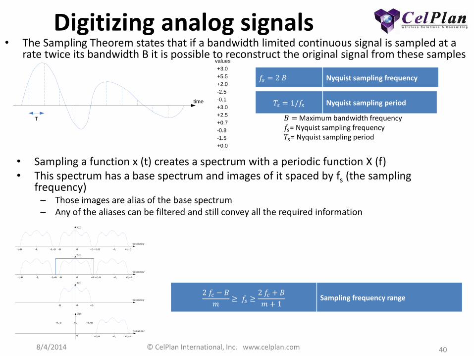
Digitizing analog signals • The Sampling Theorem states that if a bandwidth limited continuous signal is sampled at a
rate twice its bandwidth B it is possible to reconstruct the original signal from these samples
time
values
+3.0
+5.5
+2.0
-2.5
-0.1
+3.0
+2.5
+0.7
-0.8
-1.5
+0.0
T
𝑓𝑠 = 2 𝐵 Nyquist sampling frequency
𝑇𝑠 = 1/𝑓𝑠 Nyquist sampling period
𝐵 = Maximum bandwidth frequency 𝑓𝑠= Nyquist sampling frequency 𝑇𝑠= Nyquist sampling period
• Sampling a function x (t) creates a spectrum with a periodic function X (f) • This spectrum has a base spectrum and images of it spaced by fs (the sampling
frequency) – Those images are alias of the base spectrum – Any of the aliases can be filtered and still convey all the required information
+B-B +fs-fs -fs+B-fs-B +fs-B +fs+B
X(f)
frequency
X(f)
frequency
+B-B
X(f)
frequency
X(f)
frequency
+B-B +fs-fs -fs+B-fs-B +fs-B +fs+B
0
0
0
0
+fs+fs-B +fs+B
+fs+fs-B +fs+B
2 𝑓𝑐 − 𝐵
𝑚≥ 𝑓𝑠 ≥
2 𝑓𝑐 + 𝐵
𝑚 + 1 Sampling frequency range

8/4/2014 © CelPlan International, Inc. www.celplan.com 41
Digital data representation in the frequency domain (spectrum)
• We will start analyzing a single unit of information that can represent a value of 1 or zero and has duration defined by T (bit)
• First we will convert the bit a Non-Return to Zero (NRZ) format to eliminate the DC component as represented below – The bit is centered at the origin
• The Discrete Fourier Transform of this signal results in the Sinc (Sinus Cardinalis) function • The Sinc function is equivalent to the sin (x)/x function, but the value for x=0 is pre-defined as 1
A
t
A
t
1
0
1
-1
T T
1-1 1-1
𝑠𝑖𝑛𝑐 𝑇𝑓 =sin (𝑇𝜋𝑓)
𝑇𝜋𝑓 Sinc function
𝐵 =1
𝑇 Pulse Bandwidth
-0.5
0
0.5
1
-20 -10 0 10 20
po
wer
frequency (Hz)
Spectrum of a 0.5 s duration pulse (sinc function)
sinc(f)=sin Tπf/Tπf abs(1/Tπf) -0.5
0
0.5
1
-20 -10 0 10 20
po
wer
frequency (Hz)
Spectrum of a 1 s duration pulse (sinc function)
sinc(f)=sin Tπf/Tπf abs(1/Tπf)
8/4/2014 © CelPlan International, Inc. www.celplan.com 42
Orthogonal Signals
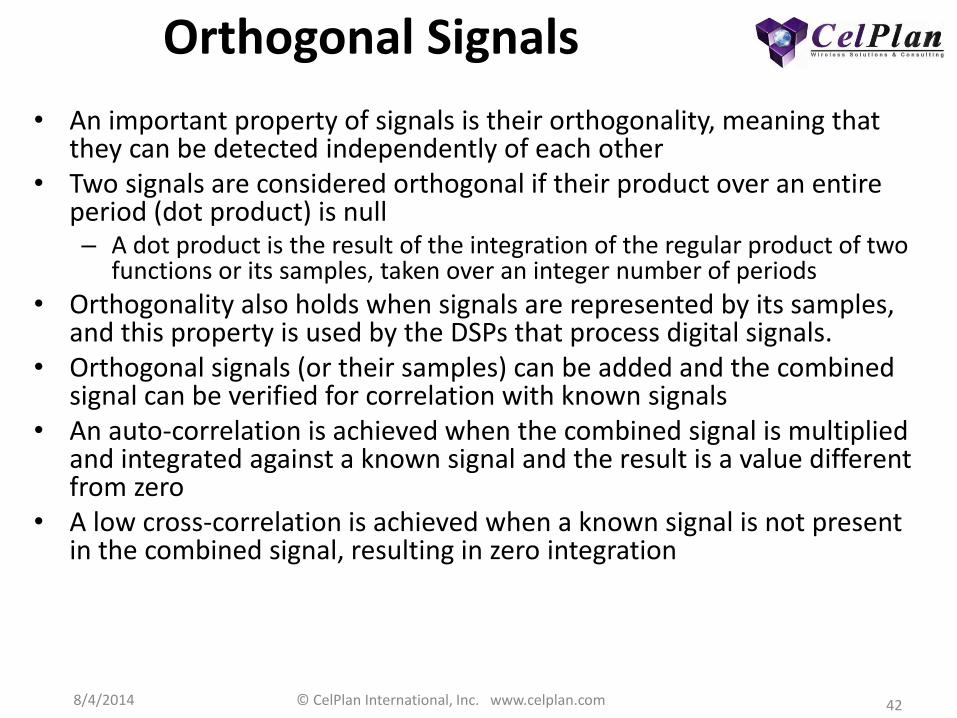
• An important property of signals is their orthogonality, meaning that they can be detected independently of each other
• Two signals are considered orthogonal if their product over an entire period (dot product) is null – A dot product is the result of the integration of the regular product of two
functions or its samples, taken over an integer number of periods
• Orthogonality also holds when signals are represented by its samples, and this property is used by the DSPs that process digital signals.
• Orthogonal signals (or their samples) can be added and the combined signal can be verified for correlation with known signals
• An auto-correlation is achieved when the combined signal is multiplied and integrated against a known signal and the result is a value different from zero
• A low cross-correlation is achieved when a known signal is not present in the combined signal, resulting in zero integration
8/4/2014 © CelPlan International, Inc. www.celplan.com 43
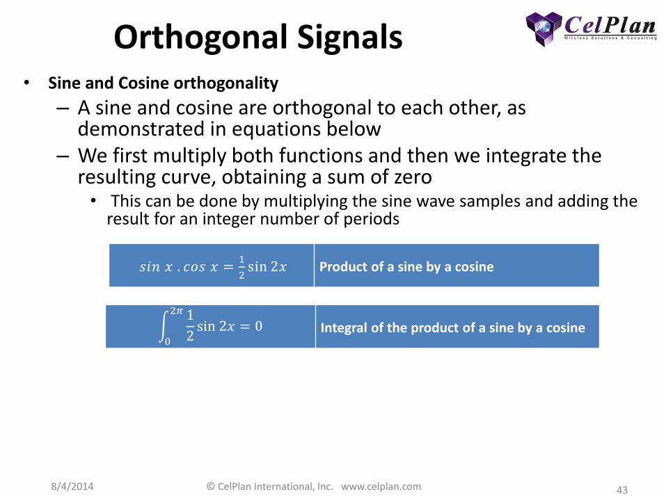
Orthogonal Signals • Sine and Cosine orthogonality
– A sine and cosine are orthogonal to each other, as demonstrated in equations below
– We first multiply both functions and then we integrate the resulting curve, obtaining a sum of zero • This can be done by multiplying the sine wave samples and adding the
result for an integer number of periods
𝑠𝑖𝑛 𝑥 . 𝑐𝑜𝑠 𝑥 =
1
2sin 2𝑥 Product of a sine by a cosine
1
2sin 2𝑥 = 0
2𝜋
0
Integral of the product of a sine by a cosine
8/4/2014 © CelPlan International, Inc. www.celplan.com 44
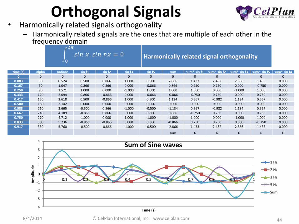
Orthogonal Signals • Harmonically related signals orthogonality
– Harmonically related signals are the ones that are multiple of each other in the frequency domain
time (s) alpha radians sin f1 sin f2 sin f3 sin f5 sum sum* sin f1 sum* sin f2 sum* sin f3 sum* sin f5 sum* sin f4
0 0 0 0 0 0 0 0 0 0 0 0 0
0.083 30 0.524 0.500 0.866 1.000 0.500 2.866 1.433 2.482 2.866 1.433 0.000
0.167 60 1.047 0.866 0.866 0.000 -0.866 0.866 0.750 0.750 0.000 -0.750 0.000
0.250 90 1.571 1.000 0.000 -1.000 1.000 1.000 1.000 0.000 -1.000 1.000 0.000
0.333 120 2.094 0.866 -0.866 0.000 -0.866 -0.866 -0.750 0.750 0.000 0.750 0.000
0.417 150 2.618 0.500 -0.866 1.000 0.500 1.134 0.567 -0.982 1.134 0.567 0.000
0.500 180 3.142 0.000 0.000 0.000 0.000 0.000 0.000 0.000 0.000 0.000 0.000
0.583 210 3.665 -0.500 0.866 -1.000 -0.500 -1.134 0.567 -0.982 1.134 0.567 0.000
0.667 240 4.189 -0.866 0.866 0.000 0.866 0.866 -0.750 0.750 0.000 0.750 0.000
0.750 270 4.712 -1.000 0.000 1.000 -1.000 -1.000 1.000 0.000 -1.000 1.000 0.000
0.833 300 5.236 -0.866 -0.866 0.000 0.866 -0.866 0.750 0.750 0.000 -0.750 0.000
0.917 330 5.760 -0.500 -0.866 -1.000 -0.500 -2.866 1.433 2.482 2.866 1.433 0.000
sum 6 6 6 6 0
-4
-3
-2
-1
0
1
2
3
4
0 0.1 0.2 0.3 0.4 0.5 0.6 0.7 0.8 0.9 1
Am
plit
ud
e
Time (s)
Sum of Sine waves
1 Hz
2 Hz
3 Hz
5 Hz
Sum
𝑠𝑖𝑛 𝑥. 𝑠𝑖𝑛 𝑛𝑥 = 02𝜋
0
Harmonically related signal orthogonality

8/4/2014 © CelPlan International, Inc. www.celplan.com 45
Combining shifted copies of a sinewave
• Combined non-orthogonal signals, such as phase-shifted copies of a sinusoidal waveform result in a sinusoidal waveform that is phase shifted itself – The final phase shift is the average of the individual components
phase shifts
-1.5
-1
-0.5
0
0.5
1
1.5
0 100 200 300 400
amp
litu
de
phase or time
Sum of shifted sinewaves 0 degree
45 degree
90 degree
135 degree
180 degree
225 degree
270 degree
sum=135 degree
-1.5
-1
-0.5
0
0.5
1
1.5
0 100 200 300 400am
plit
ud
e
phase or time
Sum of shifted and attenuated sinewaves 0 degree
45 degree
90 degree
135 degree
180 degree
225 degree
270 degree
sum=42.5 degree
8/4/2014 © CelPlan International, Inc. www.celplan.com 46
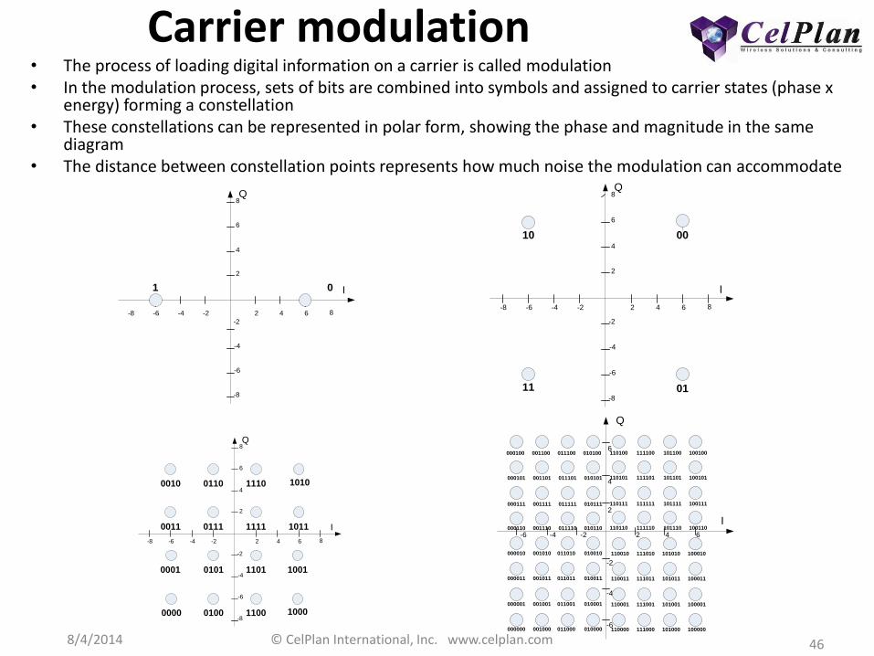
Carrier modulation • The process of loading digital information on a carrier is called modulation • In the modulation process, sets of bits are combined into symbols and assigned to carrier states (phase x
energy) forming a constellation • These constellations can be represented in polar form, showing the phase and magnitude in the same
diagram • The distance between constellation points represents how much noise the modulation can accommodate
Q
2-2 4 6 8-4-6-8
2
4
6
8
-2
-4
-6
-8
01 I
Q
2-2 4 6 8-4-6-8
2
4
6
8
-2
-4
-6
-8
00
0111
10
I
Q
2-2 4 6 8-4-6-8
2
4
6
8
-2
-4
-6
-8
1010111001100010
0011 0111 1111 1011
0001 0101 1101 1001
1000110001000000
I
Q
2-2 4 6-4-6
2
4
6
-2
-4
-6
000100 001100 011100 010100
000101 001101 011101 010101
000111 001111 011111 010111
000110 001110 011110 010110
000010 001010 011010 010010
000011 001011 011011 010011
000001 001001 011001 010001
000000 001000 011000 010000
110010 111010 101010 100010
110011 111011 101011 100011
110001 111001 101001 100001
110000 111000 101000 100000
110100 111100 101100 100100
110101 111101 101101 100101
110111 111111 101111 100111
110110 111110 101110 100110I

8/4/2014 © CelPlan International, Inc. www.celplan.com 47
Carrier modulation
-1.5
-1
-0.5
0
0.5
1
1.5
0 1 2 3 4 5Po
we
r
Symbols
BPSK modulation (Icos-Qsin) of data bits 10110
-1.5
-0.5
0.5
1.5
0 1 2 3 4 5Po
we
r
Symbols
QPSK modulation of data bits 1011000110
-1.5
-1
-0.5
0
0.5
1
1.5
2
0 1 2 3 4 5
Po
wer
Symbols
16QAM modulation of data bits 10110000101101101011
-1.5
-1
-0.5
0
0.5
1
1.5
2
0 1 2 3 4 5
Po
wer
Symbols
64QAM modulation of data bits 101010000111110110100000010101
8/4/2014 © CelPlan International, Inc. www.celplan.com 48
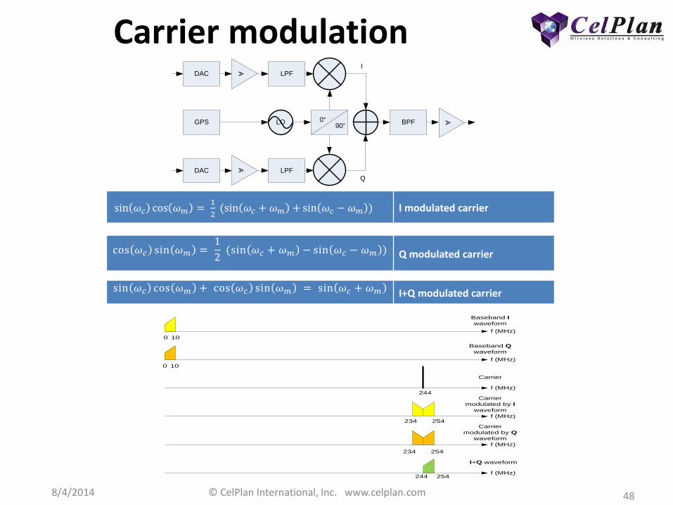
Carrier modulation DAC
A
LPF
LO
DAC
A
LPF
0°90°
BPF
A
GPS
I
Q
sin 𝜔𝑐 cos 𝜔𝑚 = 1
2 (sin 𝜔𝑐 + 𝜔𝑚 +sin 𝜔𝑐 − 𝜔𝑚 ) I modulated carrier
cos 𝜔𝑐 sin 𝜔𝑚 = 1
2 (sin 𝜔𝑐 + 𝜔𝑚 − sin 𝜔𝑐 − 𝜔𝑚 ) Q modulated carrier
sin 𝜔𝑐 cos 𝜔𝑚 + cos 𝜔𝑐 sin 𝜔𝑚 = sin 𝜔𝑐 + 𝜔𝑚 I+Q modulated carrier
f (MHz)
Baseband I
waveform
Baseband Q
waveform
Carrier
Carrier
modulated by I
waveform
I+Q waveform
Carrier
modulated by Q
waveform
0 10
0 10
244
234 254
234 254
254244
f (MHz)
f (MHz)
f (MHz)
f (MHz)
f (MHz)
8/4/2014 © CelPlan International, Inc. www.celplan.com 49
2. RF Channel

8/4/2014 © CelPlan International, Inc. www.celplan.com 50
Multipath • RF Path Characterization
– RF Multipath and Doppler effect are the main impairments on signal propagation
– It is essential to characterize multipath along the wireless deployment area
– This knowledge allows the proper wireless network design
• Multipath creates fading in time and frequency – Broader the channel larger is the
impact – A k factor prediction was developed
to indicate the expected amount of multipath
– This was ok for narrow band channels
• More accurate analysis is required for Broadband channels, like LTE
-0.500
0.000
0.500
1.000
1.500
0 5 10pro
bab
ility
den
sity
x
σ=0.5
σ=1
σ=2
σ=3

8/4/2014 © CelPlan International, Inc. www.celplan.com 51
K Factor • Signals have high coherence- High k
factor: >10 – Multipath signal follows a Gaussian
distribution
• Signals have medium coherence- Medium k factor: 10<k>2 – Multipath signal follows a Ricean
distribution
• Signals have low coherence- Low k factor: k<2 – Multipath signal follows a Rayleigh
distribution
• The k factor can be estimated on a pixel basis from the geographical data (topography and morphology) by RF prediction tools
K factor prediction
𝑘 = 10𝐹𝑠𝐹ℎ𝐹𝑏𝑑−0.5 k factor for LOS
Fs =Morphology factor (1 to 5), lower values apply to multipath rich environments Fh= Receive antenna height factor Fb=Beam width factor d = Distance hr= Receive antenna height b= Beam width in degrees
Fhhr/3)0.46 Receive antenna height factor
Fb = (b
17)−0.62 Beam width factor
𝑘 = 0 k factor for NLOS

8/4/2014 © CelPlan International, Inc. www.celplan.com 52
CelSpectrum™
CelSpectrum
• Universal Software Defined Receiver • Spectrum Capture and Analysis
– 100 MHz to 20 GHz range – Up to 100 MHz bandwidth analysis
• Spectrum Analyzer and Technology Analyzer • Multiple Technologies Decoding • Ideal for drive/walk test measurements • Captures and stores entire spectrum • Provides insights into
– Multipath – Fading – Antenna Correlation
10/27/2014 Copyright CelPlan International, Inc. 52

8/4/2014 © CelPlan International, Inc. www.celplan.com 53
CellSpectrum™ • It is an RF Spectrum and Technology RF Channel
Analyzer based on a universal software-defined receiver that enables capturing, digitizing, storing and analyzing detailed RF & technology characteristics needed for the proper design of wireless networks
• It digitizes and stores up to 100 MHz of spectrum at a time, from 100 MHz to 18 GHz, extracting parameters as: – LTE channel response per Resource Element – Multipath delay spread – Average frequency fading – Average time fading – Noise floor – Interference – Traffic Distribution – 3D visualization capability
• Additionally, allocation and traffic information can be derived, providing valuable information about the allocation used for Inter Cell Interference Coordination (ICIC). Framed OFDM transmitters, like WiMAX and LTE, provide ideal platforms to characterize the RF channel
8/4/2014 © CelPlan International, Inc. www.celplan.com 54
CellSpectrum
Spectrum Analyzer
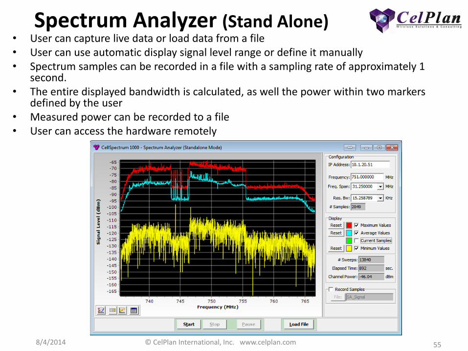
8/4/2014 © CelPlan International, Inc. www.celplan.com 55
Spectrum Analyzer (Stand Alone) • User can capture live data or load data from a file • User can use automatic display signal level range or define it manually • Spectrum samples can be recorded in a file with a sampling rate of approximately 1
second. • The entire displayed bandwidth is calculated, as well the power within two markers
defined by the user • Measured power can be recorded to a file • User can access the hardware remotely

8/4/2014 © CelPlan International, Inc. www.celplan.com 56
CellSpectrum (Drive Test)
• CellSpectrum allows to capture the spectrum along a drive test route and store it for future analysis
• This reduces the cost of collecting data and allows the analysis and re-analysis of it
• User can zoom to analyze part of the spectrum, as required
8/4/2014 © CelPlan International, Inc. www.celplan.com 57
RF Channel and Technology Analyzer
Mobile Channel characterization
Stationary Channel characterization

8/4/2014 © CelPlan International, Inc. www.celplan.com 58
LTE Received Frame (Mobile) • CellSpectrum capture • Received LOS signal after time and
frequency synchronization – 10 MHz (600 sub-carriers) – 6 frames (840 symbols): 60 ms
• Signal Level per Resource Element
• Time fading
• Frequency fading
8/4/2014 © CelPlan International, Inc. www.celplan.com 59
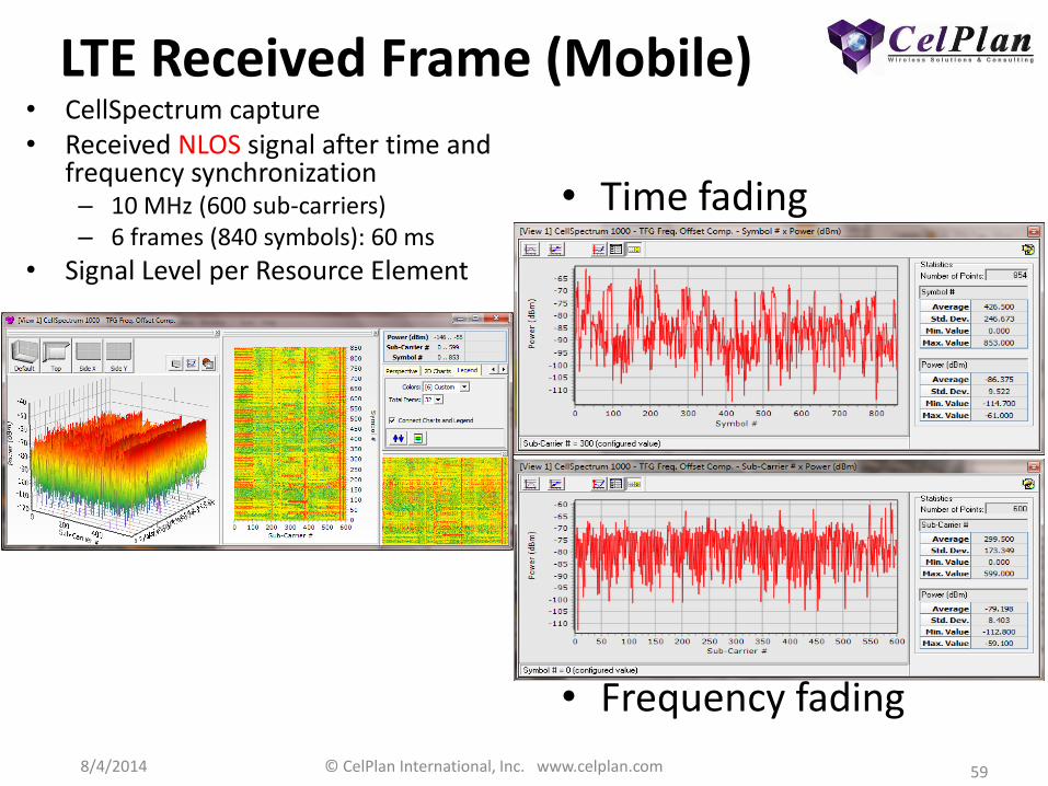
LTE Received Frame (Mobile)
• CellSpectrum capture • Received NLOS signal after time and
frequency synchronization – 10 MHz (600 sub-carriers) – 6 frames (840 symbols): 60 ms
• Signal Level per Resource Element
• Time fading
• Frequency fading

8/4/2014 © CelPlan International, Inc. www.celplan.com 60
LTE RF channel LOS • CellSpectrum capture • Received LOS signal after time and
frequency synchronization and channel equalization using pilot information – 10 MHz (600 sub-carriers) – 6 frames (840 symbols): 60 ms
• Signal Level per Resource Element
• Time fading
• Frequency fading

8/4/2014 © CelPlan International, Inc. www.celplan.com 61
LTE RF Channel NLOS
• CellSpectrum capture • Received NLOS signal after time and
frequency synchronization and channel equalization using pilot information – 10 MHz (600 sub-carriers) – 6 frames (840 symbols): 60 ms
• Signal Level per Resource Element
• Time fading
• Frequency fading
8/4/2014 © CelPlan International, Inc. www.celplan.com 62
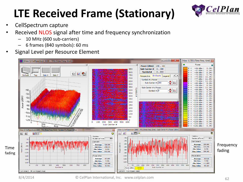
LTE Received Frame (Stationary) • CellSpectrum capture • Received NLOS signal after time and frequency synchronization
– 10 MHz (600 sub-carriers) – 6 frames (840 symbols): 60 ms
• Signal Level per Resource Element
Time fading
Frequency fading

8/4/2014 © CelPlan International, Inc. www.celplan.com 63
LTE RF Channel NLOS (stationary) • CellSpectrum capture • Received NLOS signal after time and frequency synchronization
– 10 MHz (600 sub-carriers) – 6 frames (840 symbols): 60 ms
• Signal Level per Resource Element
Time fading
Frequency fading
8/4/2014 © CelPlan International, Inc. www.celplan.com 64
3. Antenna Ports
Physical Antennas Antenna Ports
MIMO Transmission Modes

8/4/2014 © CelPlan International, Inc. www.celplan.com 65
Physical Antennas • Physical antennas are generally built from interconnected dipoles • Antennas have different radiation patterns, which are characterized in
the vertical and horizontal plane • These patterns can be modified by mechanical or electrical tilts • Antenna systems add an additional dimension to a communication
channel, as they are made from multiple antennas, providing space diversity to the RF channel
• Algorithms are then used to process transmit and receive signals to maximize the connection capacity
• Using multiple antennas creates a deployment complexity, so antenna housings are built that enclose several antennas
DD
A B C D E F G H I
8/4/2014 © CelPlan International, Inc. www.celplan.com 66
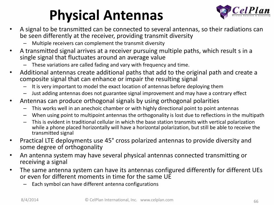
Physical Antennas • A signal to be transmitted can be connected to several antennas, so their radiations can
be seen differently at the receiver, providing transmit diversity – Multiple receivers can complement the transmit diversity
• A transmitted signal arrives at a receiver pursuing multiple paths, which result s in a single signal that fluctuates around an average value – These variations are called fading and vary with frequency and time.
• Additional antennas create additional paths that add to the original path and create a composite signal that can enhance or impair the resulting signal – It is very important to model the exact location of antennas before deploying them – Just adding antennas does not guarantee signal improvement and may have a contrary effect
• Antennas can produce orthogonal signals by using orthogonal polarities – This works well in an anechoic chamber or with highly directional point to point antennas – When using point to multipoint antennas the orthogonality is lost due to reflections in the multipath – This is evident in traditional cellular in which the base station transmits with vertical polarization
while a phone placed horizontally will have a horizontal polarization, but still be able to receive the transmitted signal
• Practical LTE deployments use 45° cross polarized antennas to provide diversity and some degree of orthogonality
• An antenna system may have several physical antennas connected transmitting or receiving a signal
• The same antenna system can have its antennas configured differently for different UEs or even for different moments in time for the same UE – Each symbol can have different antenna configurations

8/4/2014 © CelPlan International, Inc. www.celplan.com 67
Antenna Ports • The RF channel between the transmit antennas and the receive antennas has to be
characterized and equalized to extract the signal – This is done by transmitting reference signals together with the information signal
• Antenna ports are virtual antennas characterized by the reference signal being sent • The same set of physical antennas will be labeled with different port numbers if they
are characterized by a different reference signal
Antenna Port 3GPP Release Reference Signal Applications 0 to 3 8 Cell specific (CRS) Single stream transmission, transmission diversity, MIMO
4 8 MBSFN (MRS) Multimedia Broadcast Multicast Service (MBMS) 5 8 UE specific (UERS) Beamforming without MIMO
6 9 Position (PRS) Location based services
7 to 8 9 UE specific (UERS) Beamforming with MIMO; multi-user MIMO
9 to 14 10 UE specific (UERS) Beamforming with MIMO; multi-user MIMO
15 to 22 10 CSI Channel State Information (CSI) report
Uplink Antenna Port Number
Channels and Signals Antenna port index Number of antennas
1 2 4
PUSCH and DMRS-PUSCH
0 10 20 40
1 21 41
2 42
3 43
SRS
0 10 20 40
1 21 41
2 42
3 43
PUCCH and DMRS-PUCCH 0 100 200
1 201

8/4/2014 © CelPlan International, Inc. www.celplan.com 68
Multiple Input Multiple Output (MIMO)
• MIMO refers to the input and output to the RF channel • MIMO T x R, means that there are T physical transmit antennas and R receive
antennas • 3GPP divides MIMO in three categories
– Single Antenna Transmission: Relies on receiver diversity to combat fading – Transmission Diversity: Provides an additional level of diversity to combat fading – Spatial Multiplexing: Increases capacity by sending different information in
different transmission layers • Open Loop: UE sends Rank Indicator (RI) and Channel Quality Indicator (CQI) • Closed Loop: UE sends Rank Indicator (RI), Channel Quality Indicator (CQI) and Precoding
Matrix Indicator (PMI) • Multi-user:
• In the downlink the following configurations are considered – 2x2 (release 8) – 4x4 (release 8) – 8x8 (release 10)
• In the uplink the following configurations are considered: – 1x1 (release 8) – 2x2 (release 10) – 4x4 (release 10)
8/4/2014 © CelPlan International, Inc. www.celplan.com 69
4. Transmission modes
8/4/2014 © CelPlan International, Inc. www.celplan.com 70
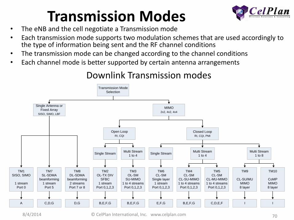
Transmission Modes • The eNB and the cell negotiate a Transmission mode • Each transmission mode supports two modulation schemes that are used accordingly to
the type of information being sent and the RF channel conditions • The transmission mode can be changed according to the channel conditions • Each channel mode is better supported by certain antenna arrangements
Single Antenna or
Fixed Array
SISO, SIMO, LBF
MIMO
2x2, 4x2, 4x4
Open Loop
RI, CQI
Closed Loop
RI, CQI, PMI
Single StreamMulti Stream
1 to 4Single Stream
Multi Stream
1 to 4
Multi Stream
1 to 8
TM1
SISO, SIMO
1 stream
Port 0
TM7
SL-SDMA
beamforming
1 stream
Port 5
TM8
DL-SDMA
beamforming
2 streams
Port 7 or 8
TM2
OL-TX DIV
SFBC
1 stream
Port 0,1,2,3
TM3
OL-SM
SU-MIMO
1 to 4 streams
Port 0,1,2,3
TM6
CL-SM
Single layer
1 stream
Port 0,1,2,3
TM4
CL-SM
CL-SU-MIMO
1 to 4 streams
Port 0,1,2,3
TM5
CL-SM
CL-MU-MIMO
1 to 4 streams
Port 0,1,2,3
TM9
CL-SU/MU
MIMO
8 layer
A
Transmission Mode
Selection
C,D,G D,G B,E,F,G B,E,F,G E,F,G B,E,F,G C,D,E,F I
TM10
CoMP
MIMO
8 layer
I
Downlink Transmission modes

8/4/2014 © CelPlan International, Inc. www.celplan.com 71
Transmission Modes DL • The eNB and the cell negotiate a Transmission mode • Each transmission mode supports two modulation schemes that are used
accordingly to the type of information being sent and the RF channel conditions
• The transmission mode can be changed according to the channel conditions • Each channel mode is better supported by certain antenna arrangements
TM Description ANTENNAS CONFIGURATION RANK PORT SISO SIMO MISO MIMO TD SM BF BF AoA OL CL SU MU
1 Single Transmit 1 A 1 0 x x x
2 Transmit Diversity 2 or 4 B,E,F,G 1 0 to 3 x x x x
3 Spatial Multiplexing 2 or 4 B,E,F,G 2 or
4 0 to 3 x x x x x
4 Spatial Multiplexing 2 or 4 B,E,F,G 2 or
4 0 to 3 x x x x x
5 MU MIMO 2 or 4 C,D,E,F 2 or
4 0 to 3 x x x x x
6 Spatial Multiplexing 2 or 4 E,F,G 2 or
4 0 to 3 x x x
7 Single Layer Beamforming ULA C,D,G 1 5 x x x x
8 Dual Layer Beamforming ULA B,E,F,G 2 7 and
8 x x x x
9 8 Layer MU MIMO 8 I 7 to 14
x x x x
10 CoMP MIMO 8 I 7 to 14
x x x
8/4/2014 © CelPlan International, Inc. www.celplan.com 72
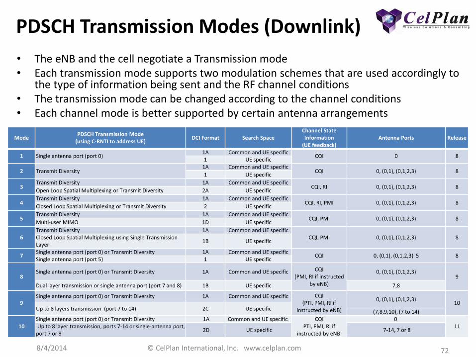
PDSCH Transmission Modes (Downlink)
• The eNB and the cell negotiate a Transmission mode • Each transmission mode supports two modulation schemes that are used accordingly to
the type of information being sent and the RF channel conditions • The transmission mode can be changed according to the channel conditions • Each channel mode is better supported by certain antenna arrangements
Mode PDSCH Transmission Mode
(using C-RNTI to address UE) DCI Format Search Space
Channel State Information
(UE feedback) Antenna Ports Release
1 Single antenna port (port 0) 1A Common and UE specific
CQI 0 8 1 UE specific
2 Transmit Diversity 1A Common and UE specific
CQI 0, (0,1), (0,1,2,3) 8 1 UE specific
3 Transmit Diversity 1A Common and UE specific
CQI, RI 0, (0,1), (0,1,2,3) 8 Open Loop Spatial Multiplexing or Transmit Diversity 2A UE specific
4 Transmit Diversity 1A Common and UE specific
CQI, RI, PMI 0, (0,1), (0,1,2,3) 8 Closed Loop Spatial Multiplexing or Transmit Diversity 2 UE specific
5 Transmit Diversity 1A Common and UE specific
CQI, PMI 0, (0,1), (0,1,2,3) 8 Multi-user MIMO 1D UE specific
6
Transmit Diversity 1A Common and UE specific
CQI, PMI 0, (0,1), (0,1,2,3) 8 Closed Loop Spatial Multiplexing using Single Transmission Layer
1B UE specific
7 Single antenna port (port 0) or Transmit Diversity 1A Common and UE specific
CQI 0, (0,1), (0,1,2,3) 5 8 Single antenna port (port 5) 1 UE specific
8 Single antenna port (port 0) or Transmit Diversity 1A Common and UE specific CQI
(PMI, RI if instructed by eNB)
0, (0,1), (0,1,2,3) 9
Dual layer transmission or single antenna port (port 7 and 8) 1B UE specific 7,8
9
Single antenna port (port 0) or Transmit Diversity 1A Common and UE specific CQI (PTI, PMI, RI if
instructed by eNB)
0, (0,1), (0,1,2,3) 10
Up to 8 layers transmission (port 7 to 14) 2C UE specific (7,8,9,10), (7 to 14)
10
Single antenna port (port 0) or Transmit Diversity 1A Common and UE specific CQI PTI, PMI, RI if
instructed by eNB
0 11 Up to 8 layer transmission, ports 7-14 or single-antenna port,
port 7 or 8 2D UE specific 7-14, 7 or 8

8/4/2014 © CelPlan International, Inc. www.celplan.com 73
PUSCH Transmission Modes (Uplink)
• The eNB and the cell negotiate a Transmission mode • Each transmission mode supports two modulation schemes that are used
accordingly to the type of information being sent and the RF channel conditions
• The transmission mode can be changed according to the channel conditions • Each channel mode is better supported by certain antenna arrangements
Mode PUSCH Transmission Scheme DCI Format Search Space Antenna Ports Release
1 Single Antenna port 0 Common and UE
specific 10 8
2
Single Antenna port 0 Common and UE
specific 10
10 Closed Loop Spatial
Multiplexing 4 UE specific (20,21), (40,41,42,43)
8/4/2014 © CelPlan International, Inc. www.celplan.com 74
5. MIMO
Multiple Input
Multiple Output
8/4/2014 © CelPlan International, Inc. www.celplan.com 75
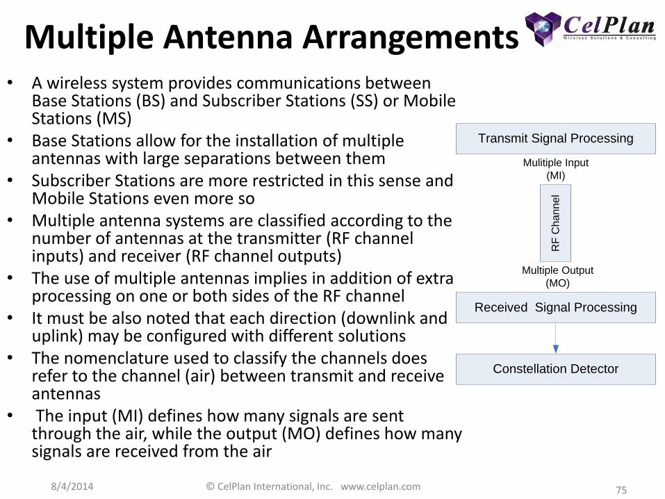
Multiple Antenna Arrangements • A wireless system provides communications between
Base Stations (BS) and Subscriber Stations (SS) or Mobile Stations (MS)
• Base Stations allow for the installation of multiple antennas with large separations between them
• Subscriber Stations are more restricted in this sense and Mobile Stations even more so
• Multiple antenna systems are classified according to the number of antennas at the transmitter (RF channel inputs) and receiver (RF channel outputs)
• The use of multiple antennas implies in addition of extra processing on one or both sides of the RF channel
• It must be also noted that each direction (downlink and uplink) may be configured with different solutions
• The nomenclature used to classify the channels does refer to the channel (air) between transmit and receive antennas
• The input (MI) defines how many signals are sent through the air, while the output (MO) defines how many signals are received from the air
Received Signal Processing
Constellation Detector
Transmit Signal Processing
RF
Ch
an
ne
l
Mulitiple Input
(MI)
Multiple Output
(MO)

8/4/2014 © CelPlan International, Inc. www.celplan.com 76
5.1 SISO
Single In Single Out
8/4/2014 © CelPlan International, Inc. www.celplan.com 77
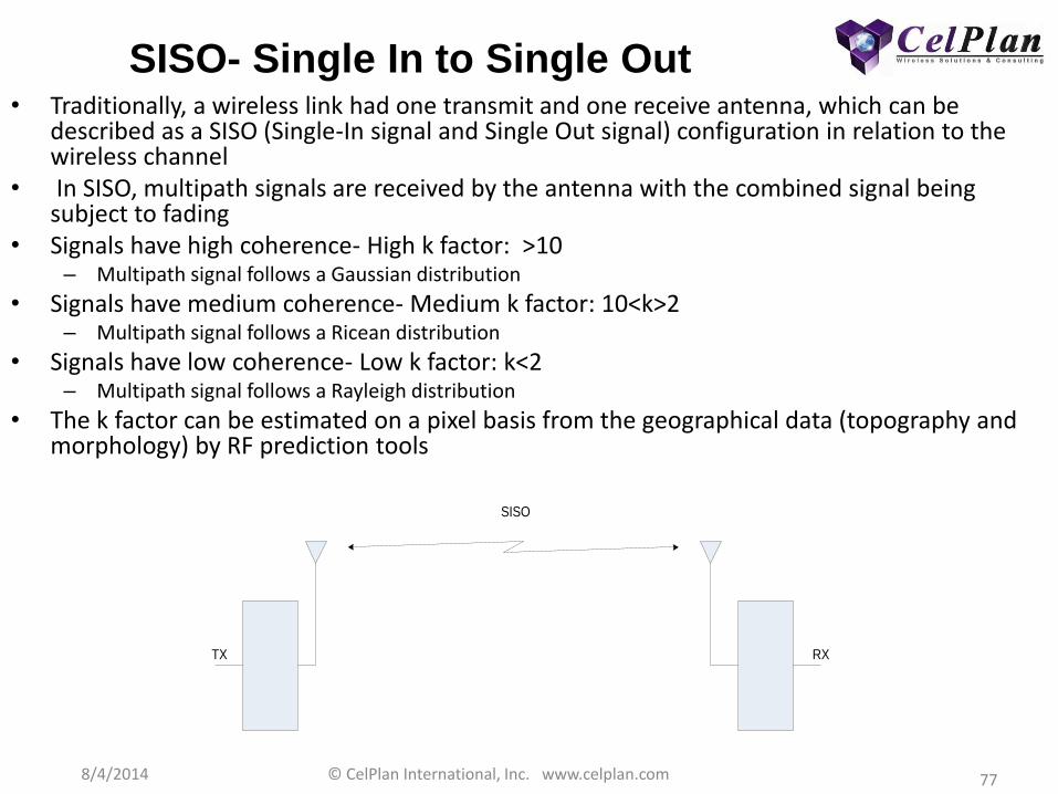
SISO- Single In to Single Out • Traditionally, a wireless link had one transmit and one receive antenna, which can be
described as a SISO (Single-In signal and Single Out signal) configuration in relation to the wireless channel
• In SISO, multipath signals are received by the antenna with the combined signal being subject to fading
• Signals have high coherence- High k factor: >10 – Multipath signal follows a Gaussian distribution
• Signals have medium coherence- Medium k factor: 10<k>2 – Multipath signal follows a Ricean distribution
• Signals have low coherence- Low k factor: k<2 – Multipath signal follows a Rayleigh distribution
• The k factor can be estimated on a pixel basis from the geographical data (topography and morphology) by RF prediction tools SISO
TX RX
8/4/2014 © CelPlan International, Inc. www.celplan.com 78
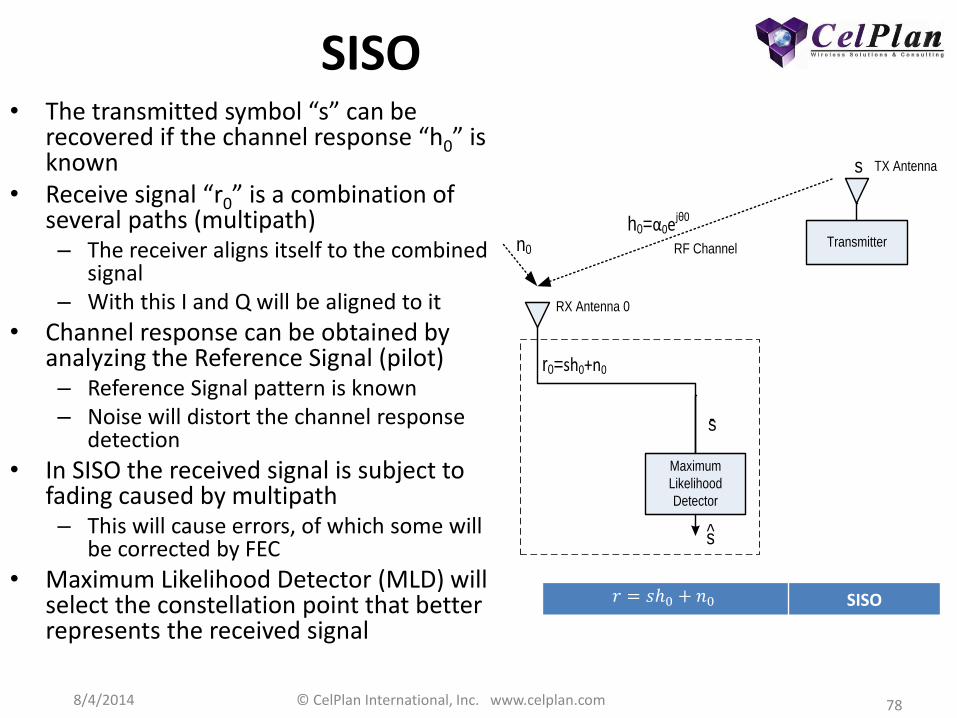
SISO • The transmitted symbol “s” can be
recovered if the channel response “h0” is known
• Receive signal “r0” is a combination of several paths (multipath) – The receiver aligns itself to the combined
signal – With this I and Q will be aligned to it
• Channel response can be obtained by analyzing the Reference Signal (pilot) – Reference Signal pattern is known – Noise will distort the channel response
detection
• In SISO the received signal is subject to fading caused by multipath – This will cause errors, of which some will
be corrected by FEC
• Maximum Likelihood Detector (MLD) will select the constellation point that better represents the received signal
𝑟 = 𝑠ℎ0 + 𝑛0 SISO
TransmitterRF Channel
s
h0=α0ejθ0
r0=sh0+n0
n0
Maximum
Likelihood
Detector
s
s
RX Antenna 0
TX Antenna

8/4/2014 © CelPlan International, Inc. www.celplan.com 79
Receiver Constellation Detection • The combined signal has to be analyzed and the constellation state detected • This detectors perform a Maximum Likelihood Detector (MLD)
• Several sub-optimal methods were developed, including: – Successive Interference Cancelation (SIC) receivers make the decision on one symbol
and subtract its effect to decide on the other symbol • This leads to error propagation
– Sphere detectors (SD) reduce the number of symbols to be analyzed by the ML detector, by performing the analysis in stages • It may preserve the optimality while reducing complexity
– Linear Detectors • Zero forcing (ZF) detectors invert the channel matrix and have small complexity but perform badly
at low SNR • Minimum Mean Square Error (MSSE) detectors reduce the combine effect of interference between
the channels and noise, but require knowledge of the SNR, which can only be roughly estimated at this stage
– More Advance Detectors • Decision Feedback (DF) or Successive Interference Cancelation (SIC) receivers make the decision on
one symbol and subtract its effect to decide on the other symbol, reducing the Inter Symbol Interference (ISI)
– This leads to error propagation
– Nearly Optimal Detectors • Sphere detectors (SD) reduce the number of symbols to be analyzed by the ML detector, by
performing the analysis in stages – It may preserve the optimality while reducing complexity

8/4/2014 © CelPlan International, Inc. www.celplan.com 80
Euclidean Distance • In mathematics, the Euclidean distance or Euclidean metric is the
"ordinary" distance between two points that one would measure with a ruler, and is given by the Pythagorean formula – In the Euclidean plane, if p = (p1, p2) and q = (q1, q2) then the distance is
given by
𝑑 𝑖, 𝑞 = (𝑖1 − 𝑞1)2+(𝑖2 − 𝑞2)
2
• Squared Euclidean distance – The standard Euclidean distance can be squared in order to place
progressively greater weight on objects that are farther apart
𝑑2 𝑖, 𝑞 = ((𝑖1 − 𝑞1)2+(𝑖2 − 𝑞2)
2
𝑑2 𝑠0, 𝑠𝑖 ≤ 𝑑2(𝑠0, 𝑠𝑘) Constellation distance
• Minimum Constellation Distance – The minimum distance (d) between a detected vector s0 and
constellation points si...sk is given by equation below – The Maximal Likelihood Detector (MLD) Searches for the
minimum constellation distance – This procedure becomes more complex as the minimum
distance has to be calculated considering that different symbols have been received from more than one antenna
Q
2-2 4 6 8-4-6-8
2
4
6
8
-2
-4
-6
-8
1010111001100010
0011 0111 1111 1011
0001 0101 1101 1001
1000110001000000
I
s0
si
sk
sj

8/4/2014 © CelPlan International, Inc. www.celplan.com 81
Maximal Likelihood Detector (MLD)
• This detector verifies the distance between the received signal and the possible constellation values, by calculating the Euclidian distance between the received signal and the possible constellation states
• The Euclidean distance is the “ordinary” distance between constellation points of a modulation and the received value
• This is an NP-hard (Non-deterministic Polynomial Time –Hard) problem
• The number of possible states can be very high, when high modulations are used, and the detection is done over multiple combinations of s symbols – A QPSK with a single symbol results in 22=4 complex operations – A 16QAM with a single symbol results in 24= 16 complex operations – A 64QAM with a single symbol results in 26=64 complex operations – A 64QAM with two symbols results in 212=4,096 complex operations – A 64QAM with four symbols results in 224=16,777,816 complex
operations

8/4/2014 © CelPlan International, Inc. www.celplan.com 82
Multiple Antennas • The techniques described next apply to both DL and UL directions, although it
is difficult to use multiple antennas in portable phones, and if implemented the antennas are generally not fully uncorrelated
• Multiple antenna techniques rely on the existence of different paths between antennas to eliminate fading. Signals with similar fading characteristics are said to be coherent, whereas signals with different fading are not coherent (or diverse).
• Co-located antennas have to be optimized to provide the desired signal diversity (no coherence), which can be done by adjusting the position or azimuth angle of the antennas. Spacing of at least λ/2 (half a wavelength) and an angular shift of at least 1/8 of the antenna beamwidth may optimize signal diversity.
• Optimizing the antennas position is not sufficient to assure non coherent signals, as the amount of LOS components in relation to indirect components has a large influence on signal coherence. LOS paths tend to be coherent, whereas non LOS paths tend to be non coherent. The amount of LOS present in a multipath signal is defined in a Ricean distribution by the k factor, which is defined as the ratio of the dominant component’s signal power over the (local-mean) scattered components power.
8/4/2014 © CelPlan International, Inc. www.celplan.com 83
5.2 SIMO
Single In
Multiple Out
8/4/2014 © CelPlan International, Inc. www.celplan.com 84
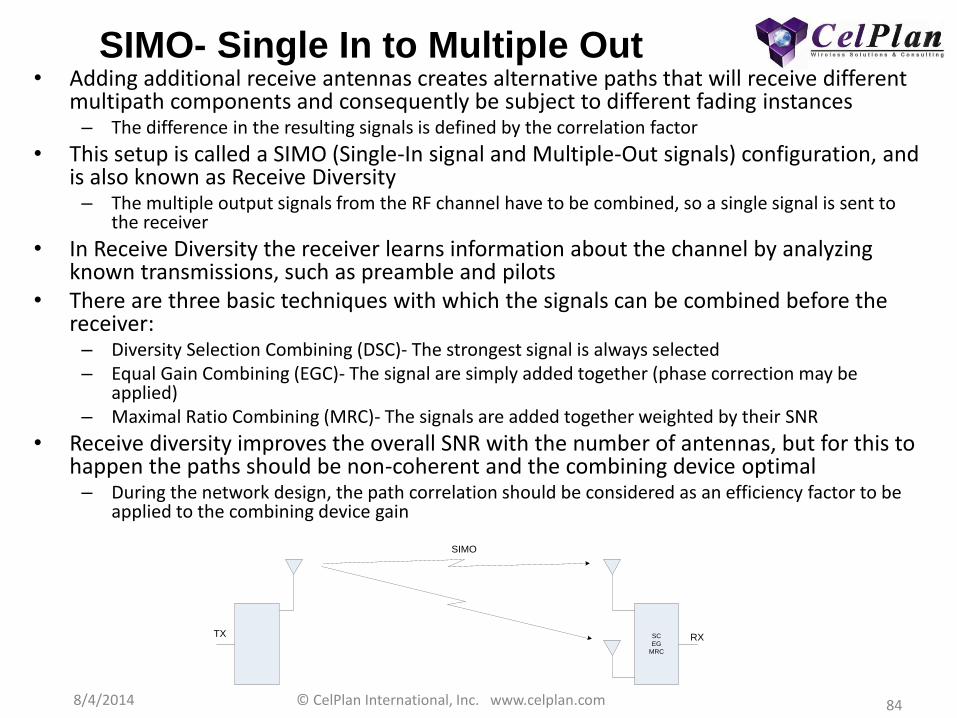
SIMO- Single In to Multiple Out • Adding additional receive antennas creates alternative paths that will receive different
multipath components and consequently be subject to different fading instances – The difference in the resulting signals is defined by the correlation factor
• This setup is called a SIMO (Single-In signal and Multiple-Out signals) configuration, and is also known as Receive Diversity – The multiple output signals from the RF channel have to be combined, so a single signal is sent to
the receiver
• In Receive Diversity the receiver learns information about the channel by analyzing known transmissions, such as preamble and pilots
• There are three basic techniques with which the signals can be combined before the receiver: – Diversity Selection Combining (DSC)- The strongest signal is always selected – Equal Gain Combining (EGC)- The signal are simply added together (phase correction may be
applied) – Maximal Ratio Combining (MRC)- The signals are added together weighted by their SNR
• Receive diversity improves the overall SNR with the number of antennas, but for this to happen the paths should be non-coherent and the combining device optimal – During the network design, the path correlation should be considered as an efficiency factor to be
applied to the combining device gain
SC
EG
MRC
SIMO
TX RX
8/4/2014 © CelPlan International, Inc. www.celplan.com 85
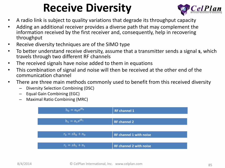
Receive Diversity • A radio link is subject to quality variations that degrade its throughput capacity • Adding an additional receiver provides a diverse path that may complement the
information received by the first receiver and, consequently, help in recovering throughput
• Receive diversity techniques are of the SIMO type • To better understand receive diversity, assume that a transmitter sends a signal s, which
travels through two different RF channels • The received signals have noise added to them in equations • This combination of signal and noise will then be received at the other end of the
communication channel • There are three main methods commonly used to benefit from this received diversity
– Diversity Selection Combining (DSC) – Equal Gain Combining (EGC) – Maximal Ratio Combining (MRC)
h0 = α0ejθ0 RF channel 1
h1 = α1ejθ1 RF channel 2
𝑟0 = 𝑠ℎ0 + 𝑛0 RF channel 1 with noise
𝑟1 = 𝑠ℎ1 + 𝑛1 RF channel 2 with noise
8/4/2014 © CelPlan International, Inc. www.celplan.com 86
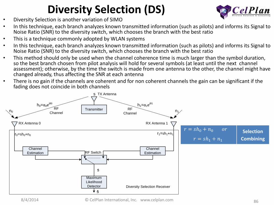
Diversity Selection (DS) • Diversity Selection is another variation of SIMO • In this technique, each branch analyzes known transmitted information (such as pilots) and informs its Signal to
Noise Ratio (SNR) to the diversity switch, which chooses the branch with the best ratio • This is a technique commonly adopted by WLAN systems • In this technique, each branch analyzes known transmitted information (such as pilots) and informs its Signal to
Noise Ratio (SNR) to the diversity switch, which chooses the branch with the best ratio • This method should only be used when the channel coherence time is much larger than the symbol duration,
so the best branch chosen from pilot analysis will hold for several symbols (at least until the next channel assessment); otherwise, by the time the switch is made from one antenna to the other, the channel might have changed already, thus affecting the SNR at each antenna
• There is no gain if the channels are coherent and for non coherent channels the gain can be significant if the fading does not coincide in both channels
𝑟 = 𝑠ℎ0 + 𝑛0 𝑜𝑟
𝑟 = 𝑠ℎ1 + 𝑛1
Selection
Combining
Transmitter
Channel
Estimation
Channel
Estimation
RF
ChannelRF
Channel
s
h1=α1ejθ1h0=α0ejθ0
n0 n1
r0=sh0+n0r1=sh1+n1
RF Switch
Diversity Selection Receiver
Maximum
Likelihood
Detector
s
s
RX Antenna 0 RX Antenna 1
TX Antenna

8/4/2014 © CelPlan International, Inc. www.celplan.com 87
Equal Gain Combining (EGC) • Equal Gain Combining is illustrated below • The signals received from both branches are combined, as expressed in the equation
– Each branch should have its own LNA, to avoid combiner loss
• For coherent channels (identical or nearly identical), there is no real gain as the signal and the noise rise together by 3 dB, that is, even though there was an increase in the signal (added twice), there was exactly the same increase in noise, thus ir results in the same as receiving in only one antenna, i.e. no diversity
• For non coherent channels there is a significant gain when fading occurs in one channel and not in the other
• This solution is the easiest type of receive diversity to implement, but the benefit only happens when the probability of fading overlap between the channels is small – The use of different polarizations for the Rx antennas helps to maximize this benefit
𝑟 = 𝑠 ℎ0 + ℎ1 + 𝑛𝑜 + 𝑛1 Equal Gain
Combining
TransmitterRF Channel RF Channel
s
h1=α1ejθ1h0=α0ejθ0
r0=sh0+n0r1=sh1+n1
n1n0
Equal Gain Combining Receiver
Maximum
Likelihood
Detector
s
s
RX Antenna 0 RX Antenna 1
TX Antenna
8/4/2014 © CelPlan International, Inc. www.celplan.com 88
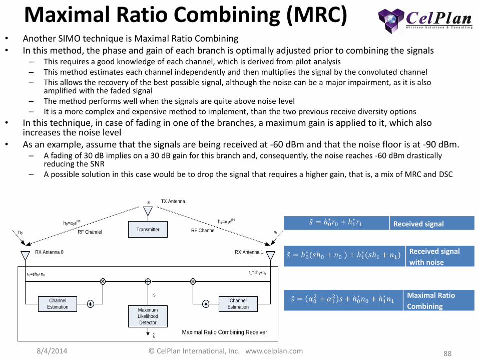
Maximal Ratio Combining (MRC) • Another SIMO technique is Maximal Ratio Combining • In this method, the phase and gain of each branch is optimally adjusted prior to combining the signals
– This requires a good knowledge of each channel, which is derived from pilot analysis – This method estimates each channel independently and then multiplies the signal by the convoluted channel – This allows the recovery of the best possible signal, although the noise can be a major impairment, as it is also
amplified with the faded signal – The method performs well when the signals are quite above noise level – It is a more complex and expensive method to implement, than the two previous receive diversity options
• In this technique, in case of fading in one of the branches, a maximum gain is applied to it, which also increases the noise level
• As an example, assume that the signals are being received at -60 dBm and that the noise floor is at -90 dBm. – A fading of 30 dB implies on a 30 dB gain for this branch and, consequently, the noise reaches -60 dBm drastically
reducing the SNR – A possible solution in this case would be to drop the signal that requires a higher gain, that is, a mix of MRC and DSC
𝑠 = ℎ0∗𝑟0 + ℎ1
∗𝑟1 Received signal
𝑠 = ℎ0∗(𝑠ℎ0 + 𝑛0 ) + ℎ1
∗(𝑠ℎ1 + 𝑛1) Received signal
with noise
𝑠 = 𝛼02 + 𝛼1
2 𝑠 + ℎ0∗𝑛0 + ℎ1
∗𝑛1 Maximal Ratio
Combining
Transmitter
Channel
Estimation
Channel
EstimationMaximum
Likelihood
Detector
RF Channel RF Channel
s
h1=α1ejθ1h0=α0ejθ0
n0 n1
r0=sh0+n0r1=sh1+n1
s
Maximal Ratio Combining Receiver
RX Antenna 0 RX Antenna 1
TX Antenna
^s

8/4/2014 © CelPlan International, Inc. www.celplan.com 89
5.3 MISO
Multiple In
Single Out

8/4/2014 © CelPlan International, Inc. www.celplan.com 90
MISO- Multiple In to Single Out • Adding additional transmit antennas creates alternative paths that will have different multipath components
and, consequently, be subject to different fading instances – The amount of difference in the resulting signals is defined by the coherence factor
• Multiple transmit antenna configurations are called MISO (Multiple-In signal and Single-Out signal), and are also known as Transmit Diversity
• The receive antenna receives signals coming from two or more transmit antennas, so, in principle, it receives n times the power, n being the number of transmit antennas
• This gain in power is known as the Array Gain and can be positive or negative (representing a loss) depending on the signal coherence – The signal coherence is a direct function of the antenna correlation
• There are two modes of transmitting schemes for MISO: open loop, and closed loop. – In open loop, the transmitter does not have any information about the channel – In closed loop, the receiver sends Channel State Information (CSI) to the transmitter on a regular basis
• The transmitter uses this information to adjust its transmissions using one of the methods below.
• There are two main configurations for Transmit Diversity: – Transmit Channel Diversity- The transmitter evaluates periodically the antenna that gives best results and transmits on it
• Only one antenna transmits a time.
– Transmit Redundancy- A linear pre-coding is applied at the transmitter and a post-coder is used at the receiver, both using the CSI information
• Both antennas transmit simultaneously
• Additional transmit diversity can only be obtained by replacing sets of multiple symbols by orthogonal signals and transmitting each orthogonal symbol on a different antenna – Alamouti proposed an orthogonal code for two symbol blocks in a method called Space Time Block Coding (STBC) – 3GPP specifies a similar solution but replacing time by frequency, in a method called Space Frequency Block Coding (SFBC) – This method does not improve overall SNR, but reduces it by averaging the fading over two symbols or two sub-carriers
STC
MISO
TX RX

8/4/2014 © CelPlan International, Inc. www.celplan.com 91
Transmit Diversity • The addition of more transmitters creates new multipath and may increase the
detection options in a method known • Transmit diversity can be represented by a matrix that relates data send in the
antennas to a certain sequence of symbols – n :transmit antennas – T :Symbols(represents the transmit diversity block size) – sij :modulated symbol
• This matrix is defined by a code rate that expresses the number of symbols that can be transmitted on the course of one block
• A block that encodes k symbols has its code rate defined by the equation below • The three, most common types of transmit diversity techniques are:
– Receiver based Transmit Selection – Transmit Redundancy – Space Time Transmit Diversity – Space Time Block Code (Alamouti’s code or Matrix A) – Transmit and Receive Diversity – Spatial Multiplexing (Matrix B)
𝑟 =𝑘
𝑇 Matrix code rate
𝑠11 ⋯ 𝑠1𝑛⋮ ⋱ ⋮𝑠𝑇1 ⋯ 𝑠𝑇𝑛
Transmit antennas
Sym
bo
ls
𝑎𝑖𝑗 𝑖 = 𝑟𝑜𝑤 (Symbol) 𝑗 = 𝑐𝑜𝑙𝑢𝑚𝑛 (Antenna)

8/4/2014 © CelPlan International, Inc. www.celplan.com 92
Receiver based Transmit Selection
• In TDD systems, transmit and receive directions use the same channel • When channels vary very slowly, it is reasonable to assume that the
best channel used for the receive side would be the best one to transmit as well
• However, this only holds true for channels with coherence time larger than the frame time 𝑟 = 𝑠0ℎ0 + 𝑛 𝑜𝑟 𝑟 = 𝑠1ℎ1 + 𝑛 Received based transmit selection
Transmitter
RF ChannelRF Channel
s
h1=α1ejθ1h0=α0ejθ0
nTransmitter
s
Maximum Likelihood Detector
TX Antenna 0 TX Antenna 1
RX Antenna
s
Receiver Based Transmit Selection
8/4/2014 © CelPlan International, Inc. www.celplan.com 93
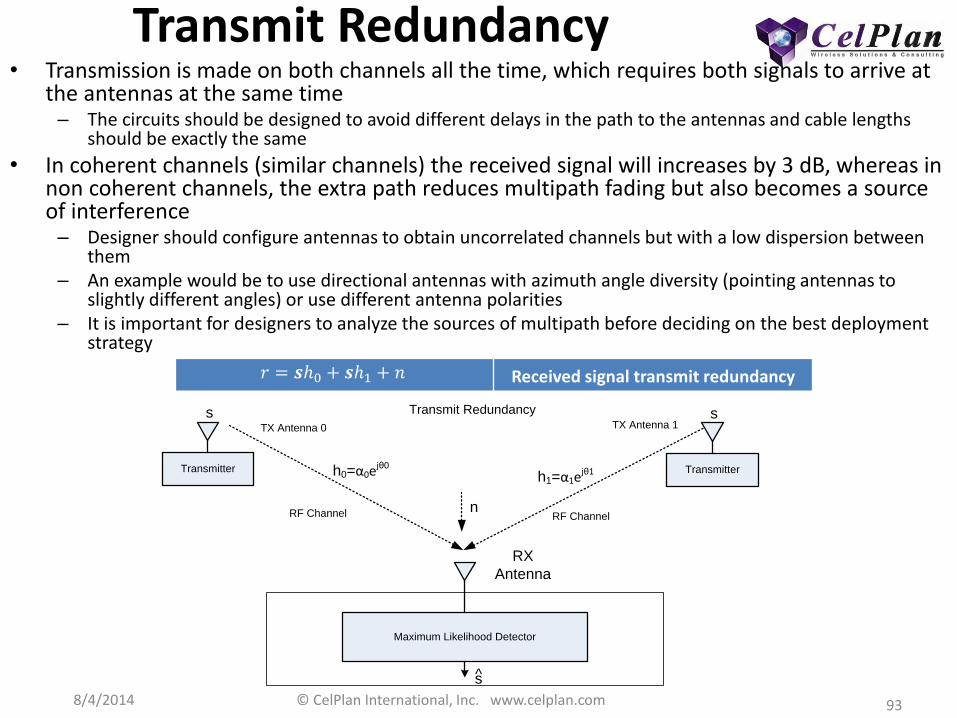
Transmit Redundancy • Transmission is made on both channels all the time, which requires both signals to arrive at
the antennas at the same time – The circuits should be designed to avoid different delays in the path to the antennas and cable lengths
should be exactly the same
• In coherent channels (similar channels) the received signal will increases by 3 dB, whereas in non coherent channels, the extra path reduces multipath fading but also becomes a source of interference – Designer should configure antennas to obtain uncorrelated channels but with a low dispersion between
them – An example would be to use directional antennas with azimuth angle diversity (pointing antennas to
slightly different angles) or use different antenna polarities – It is important for designers to analyze the sources of multipath before deciding on the best deployment
strategy
𝑟 = 𝒔ℎ0 + 𝒔ℎ1 + 𝑛 Received signal transmit redundancy
Transmitter
RF ChannelRF Channel
s
h1=α1ejθ1h0=α0ejθ0
n
Transmitter
s
Maximum Likelihood Detector
TX Antenna 0 TX Antenna 1
RX
Antenna
s
Transmit Redundancy
8/4/2014 © CelPlan International, Inc. www.celplan.com 94
Space Time Transmit Diversity • Additional schemes of SIMO that add a time component to the
space diversity provided by multiple antennas have also been proposed
• Some examples are: – Delay Diversity and – Space Time Trellis
• Both methods rely on creating additional multipath and are complex to implement
• A simpler method was proposed by Siavash Alamouti • On his proposition, the multipath is delayed by a full symbol, and
then a conjugate value is sent to cancel the reactive part of the signal – This technique is easy to implement, but requires the channel to remain
stable over a period of two symbols – This means that the coherence time should be larger than two symbols – This method is called Space-Time Block Coding (STBC or STC), also
known as Matrix A

8/4/2014 © CelPlan International, Inc. www.celplan.com 95
Space Time Block Code-Alamouti‘s code (Matrix A)
• In this technique, each transmission block is made of two symbols in time
• Each antenna sends the information as depicted in the table below – The operations applied over the information were carefully chosen
to cancel the unwanted information at each antenna – In this technique, even though different information is sent by each
antenna on one symbol, the same information is repeated over the next symbol, thus this is still considered a diversity scheme
• This is the only type of code that can reach a coding rate of 1 – In the WiMAX standard, this matrix is referred to as Matrix A – Equation below shows how the matrix is built – BS support of this method is mandatory in the WiMAX and LTE
standards
𝑋 =𝑠0 𝑠1−𝑠1∗ 𝑠0∗ Matrix A
Alamouti Antenna 0 Antenna 1
Symbol 0 S0 S1
Symbol 1 -S1* S0
*
8/4/2014 © CelPlan International, Inc. www.celplan.com 96
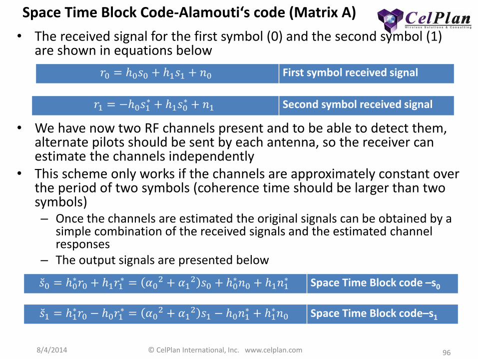
Space Time Block Code-Alamouti‘s code (Matrix A)
• The received signal for the first symbol (0) and the second symbol (1) are shown in equations below 𝑟0 = ℎ0𝑠0 + ℎ1𝑠1 + 𝑛0 First symbol received signal
𝑟1 = −ℎ0𝑠1∗ + ℎ1𝑠0
∗ + 𝑛1 Second symbol received signal
• We have now two RF channels present and to be able to detect them, alternate pilots should be sent by each antenna, so the receiver can estimate the channels independently
• This scheme only works if the channels are approximately constant over the period of two symbols (coherence time should be larger than two symbols) – Once the channels are estimated the original signals can be obtained by a
simple combination of the received signals and the estimated channel responses
– The output signals are presented below
𝑠 0 = ℎ0∗𝑟0 + ℎ1𝑟1
∗ = 𝛼02 + 𝛼1
2 𝑠0 + ℎ0∗𝑛0 + ℎ1𝑛1
∗ Space Time Block code –s0
𝑠 1 = ℎ1∗𝑟0 − ℎ0𝑟1
∗ = 𝛼02 + 𝛼1
2 𝑠1 − ℎ0𝑛1∗ + ℎ1∗𝑛0 Space Time Block code–s1
8/4/2014 © CelPlan International, Inc. www.celplan.com 97
Space Time Block Code-Alamouti‘s code (Matrix A)
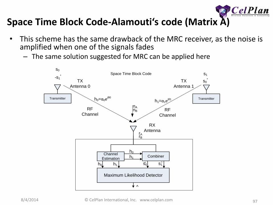
• This scheme has the same drawback of the MRC receiver, as the noise is amplified when one of the signals fades – The same solution suggested for MRC can be applied here
Transmitter
Channel
Estimation
RF
Channel
RF
Channel
-s1*
h1=α1ejθ1h0=α0ejθ0 Transmitter
s1
Combiner
Maximum Likelihood Detector
h0
h1
h1h0 s0 s1
s0
s0*
nAnB
rArB
TX
Antenna 0
TX
Antenna 1
RX
Antenna
^
Space Time Block Code
8/4/2014 © CelPlan International, Inc. www.celplan.com 98
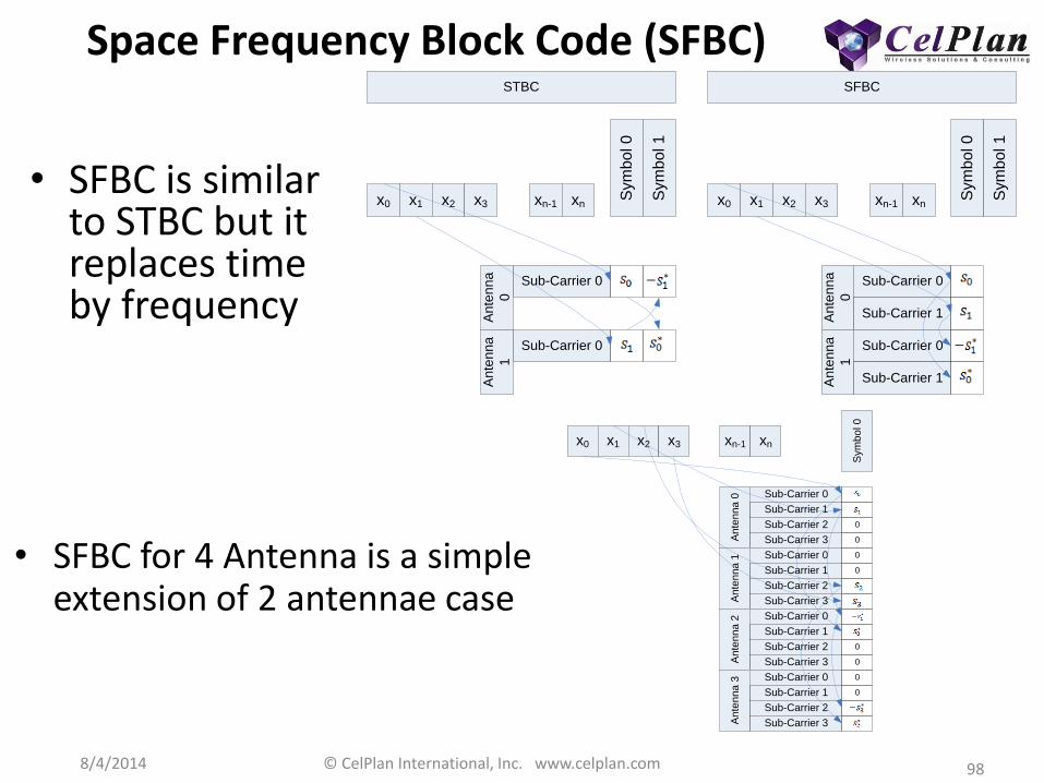
Space Frequency Block Code (SFBC)
• SFBC is similar to STBC but it replaces time by frequency
• SFBC for 4 Antenna is a simple extension of 2 antennae case
x0 x1 x2 x3 xn-1 xn
Sub-Carrier 0
Sym
bo
l 0
An
ten
na
0
Sub-Carrier 1
Sub-Carrier 0
An
ten
na
1
Sub-Carrier 1
Sub-Carrier 0
An
ten
na
0
Sub-Carrier 0
An
ten
na
1
x0 x1 x2 x3 xn-1 xn
Sym
bo
l 1
SFBC
Sym
bo
l 0
Sym
bo
l 1
STBC
Sub-Carrier 0
An
ten
na
0
Sub-Carrier 1
Sub-Carrier 2
Sub-Carrier 3
Sub-Carrier 0
An
ten
na
1
Sub-Carrier 1
Sub-Carrier 2
Sub-Carrier 3
Sub-Carrier 0
An
ten
na
2
Sub-Carrier 1
Sub-Carrier 2
Sub-Carrier 3
Sub-Carrier 0
An
ten
na
3
Sub-Carrier 1
Sub-Carrier 2
Sub-Carrier 3
x0 x1 x2 x3 xn-1 xn
0
0
0
0
0
0
0
0
Sym
bo
l 0
8/4/2014 © CelPlan International, Inc. www.celplan.com 99
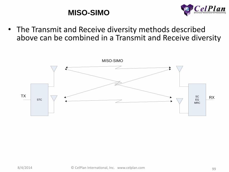
MISO-SIMO
• The Transmit and Receive diversity methods described above can be combined in a Transmit and Receive diversity
SC
EG
MRC
STC
MISO-SIMO
TX RX

8/4/2014 © CelPlan International, Inc. www.celplan.com 100
Transmit and Receive Diversity (TRD) • Transmit diversity can be mixed with MRC to provide a fourth order diversity MIMO scheme
(2x2) as can be seen in figure and equations below 𝑟0 = ℎ0𝑠0 + ℎ1𝑠1 + 𝑛0 TRD received signal 0
𝑟1 = −ℎ0𝑠1∗ − ℎ1𝑠0
∗ + 𝑛1 TRD received signal 1
𝑟2 = ℎ2𝑠0 + ℎ3𝑠1 + 𝑛2 TRD received signal 2
𝑟3 = −ℎ2𝑠1∗ + ℎ3𝑠0
∗ + 𝑛3 TRD received signal 3
𝑠 0 = ℎ0∗𝑟0 + ℎ1𝑟1
∗ + ℎ2∗𝑟2 + ℎ3𝑟3
∗ = 𝛼02 + 𝛼1
2 + 𝛼22 + 𝛼3
2 𝑠0 + ℎ0∗𝑛0 + ℎ1𝑛1
∗ + ℎ2∗𝑛2 + ℎ3𝑛3
∗ TRD output signal 0
𝑠 1 = ℎ1∗𝑟0 − ℎ0𝑟1
∗ +ℎ3∗ 𝑟2 − ℎ2𝑟3
∗ = 𝛼02 + 𝛼1
2 + 𝛼22 + 𝛼3
2 𝑠1 − ℎ0𝑛1∗ + ℎ1∗𝑛0 − ℎ2𝑛3
∗ + ℎ3∗𝑛2 TRD output signal 1
Transmitter
Channel
Estimation
RF ChannelRF Channel
-s1*
h01=α01ejθ01
h00=α00ejθ
00
Transmitter
s1
Combiner
Maximum Likelihood Detector
h00
h01
h01h00 sA sB
s0
s0*
n0An0B
r0Ar0B
Channel
Estimation
h11h10
n1B
n1A
h10=α10ejθ10
h11=α11ejθ
11
h10
h11
r1Ar1B
^sA sB
RX Antenna 0 RX Antenna 1
TX Antenna 1TX Antenna 0

8/4/2014 © CelPlan International, Inc. www.celplan.com 101
5.4 MIMO
8/4/2014 © CelPlan International, Inc. www.celplan.com 102
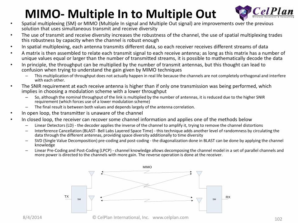
MIMO- Multiple In to Multiple Out • Spatial multiplexing (SM) or MIMO (Multiple In signal and Multiple Out signal) are improvements over the previous
solution that uses simultaneous transmit and receive diversity • The use of transmit and receive diversity increases the robustness of the channel, the use of spatial multiplexing trades
this robustness by capacity when the channel is robust enough • In spatial multiplexing, each antenna transmits different data, so each receiver receives different streams of data • A matrix is then assembled to relate each transmit signal to each receive antenna; as long as this matrix has a number of
unique values equal or larger than the number of transmitted streams, it is possible to mathematically decode the data • In principle, the throughput can be multiplied by the number of transmit antennas, but this thought can lead to
confusion when trying to understand the gain given by MIMO techniques – This multiplication of throughput does not actually happen in real life because the channels are not completely orthogonal and interfere
with each other.
• The SNIR requirement at each receive antenna is higher than if only one transmission was being performed, which implies in choosing a modulation scheme with a lower throughput – So, although the nominal throughput of the link is multiplied by the number of antennas, it is reduced due to the higher SNIR
requirement (which forces use of a lower modulation scheme) – The final result is between both values and depends largely of the antenna correlation.
• In open loop, the transmitter is unaware of the channel • In closed loop, the receiver can recover some channel information and applies one of the methods below
– Linear Detectors (LD) - the decoder applies the inverse of the channel to amplify it, trying to remove the channel distortions – Interference Cancellation (BLAST- Bell Labs Layered Space Time) - this technique adds another level of randomness by circulating the
data through the different antennas, providing space diversity additionally to time diversity – SVD (Single Value Decomposition) pre-coding and post-coding - the diagonalization done in BLAST can be done by applying the channel
knowledge – Linear Pre-Coding and Post-Coding (LPCP) - channel knowledge allows decomposing the channel model in a set of parallel channels and
more power is directed to the channels with more gain. The reverse operation is done at the receiver.
SMSM
MIMO
TX RX
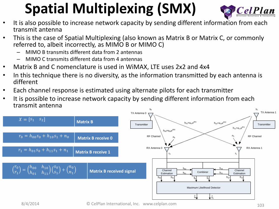
8/4/2014 © CelPlan International, Inc. www.celplan.com 103
Spatial Multiplexing (SMX) • It is also possible to increase network capacity by sending different information from each
transmit antenna • This is the case of Spatial Multiplexing (also known as Matrix B or Matrix C, or commonly
referred to, albeit incorrectly, as MIMO B or MIMO C) – MIMO B transmits different data from 2 antennas – MIMO C transmits different data from 4 antennas
• Matrix B and C nomenclature is used in WiMAX, LTE uses 2x2 and 4x4 • In this technique there is no diversity, as the information transmitted by each antenna is
different • Each channel response is estimated using alternate pilots for each transmitter • It is possible to increase network capacity by sending different information from each
transmit antenna
𝑋 = 𝑠1 𝑠2 Matrix B
𝑟0 = ℎ00𝑠0 + ℎ10𝑠1 + 𝑛0 Matrix B receive 0
𝑟1 = ℎ01𝑠0 + ℎ11𝑠1 + 𝑛1 Matrix B receive 1
𝑟0𝑟1=ℎ00 ℎ10ℎ01 ℎ11
𝑠0𝑠1+𝑛0𝑛1
Matrix B received signal
Transmitter
Channel
Estimation
RF ChannelRF Channel
h01=α01ejθ01
h00=α00ejθ00
Transmitter
s1
Combiner
Maximum Likelihood Detector
h00
h01
h01h00 s0 s1
s0
n0
r0
Channel
Estimation
h11h10
n1
h10=α10ejθ10
h11=α11ejθ11
h10
h11
r1
s0 s1
RX Antenna 0 RX Antenna 1
TX Antenna 0 TX Antenna 1
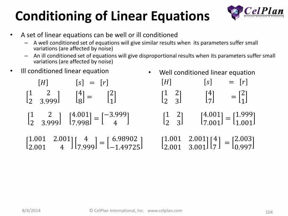
8/4/2014 © CelPlan International, Inc. www.celplan.com 104
Conditioning of Linear Equations
• Ill conditioned linear equation
𝐻 𝑠 = 𝑟
1 22 3.999
48=
21
• A set of linear equations can be well or ill conditioned – A well conditioned set of equations will give similar results when its parameters suffer small
variations (are affected by noise) – An ill conditioned set of equations will give disproportional results when its parameters suffer small
variations (are affected by noise)
1 22 3.999
4.0017.998
=−3.9994
1.001 2.0012.001 4
47.999
=6.98902−1.49725
• Well conditioned linear equation
𝐻 𝑠 = 𝑟
1 22 3
47 =
21
1 22 3 4.0017.001
=1.9991.001
1.001 2.0012.001 3.001
47 =2.0030.997
8/4/2014 © CelPlan International, Inc. www.celplan.com 105
Condition Number • In the field of numerical analysis, the condition number of a function with
respect to an argument measures how much the output value of the function can change for a small change in the input argument – This is used to measure how sensitive a function is to changes or errors in the
input, and how much error in the output results from an error in the input – A problem with a low condition number is said to be well-conditioned, while a
problem with a high condition number is said to be ill-conditioned. The condition number is a property of the problem
• A system of equations is considered to be well-conditioned if a small change in the coefficient matrix or a small change in the right hand side results in a small change in the solution vector
• A system of equations is considered to be ill-conditioned if a small change in the coefficient matrix or a small change in the right hand side results in a large change in the solution vector
• Every invertible square matrix has a condition number and coupled with the machine epsilon, it is possible to quantify how many digits can be trusted in the solution
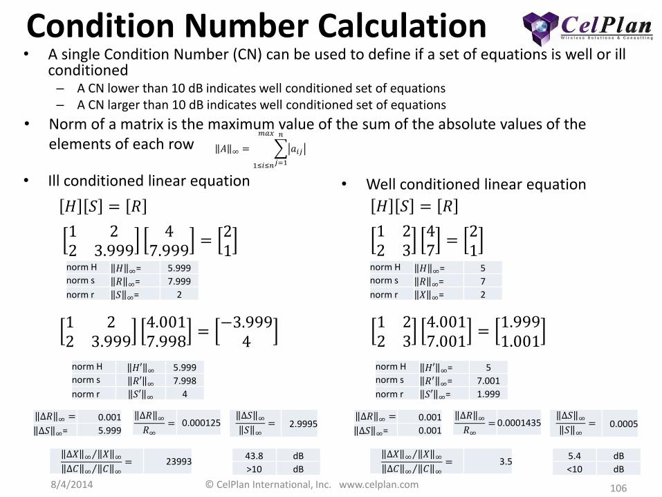
8/4/2014 © CelPlan International, Inc. www.celplan.com 106
Condition Number Calculation
• Ill conditioned linear equation
𝐻 𝑆 = 𝑅
1 22 3.999
47.999
=21
• A single Condition Number (CN) can be used to define if a set of equations is well or ill conditioned – A CN lower than 10 dB indicates well conditioned set of equations – A CN larger than 10 dB indicates well conditioned set of equations
1 22 3.999
4.0017.998
=−3.9994
• Well conditioned linear equation
𝐻 𝑆 = 𝑅
1 22 347=21
1 22 34.0017.001
=1.9991.001
norm H 𝐻 ∞= 5.999 norm s 𝑅 ∞= 7.999
norm r 𝑆 ∞= 2
norm H 𝐻 ∞= 5 norm s 𝑅 ∞= 7
norm r 𝑋 ∞= 2
• Norm of a matrix is the maximum value of the sum of the absolute values of the elements of each row
norm H 𝐻′ ∞ 5.999 norm s 𝑅′ ∞ 7.998
norm r 𝑆′ ∞ 4
norm H 𝐻′ ∞= 5 norm s 𝑅′ ∞= 7.001
norm r 𝑆′ ∞= 1.999
Δ𝑅 ∞ = 0.001
Δ𝑆 ∞= 5.999
Δ𝑅 ∞𝑅∞= 0.000125
Δ𝑆 ∞𝑆 ∞= 2.9995
Δ𝑋 ∞ 𝑋 ∞
Δ𝐶 ∞ 𝐶 ∞ = 23993
43.8 dB
>10 dB
Δ𝑅 ∞ = 0.001
Δ𝑆 ∞= 0.001
Δ𝑅 ∞𝑅∞= 0.0001435
Δ𝑆 ∞𝑆 ∞= 0.0005
Δ𝑋 ∞ 𝑋 ∞
Δ𝐶 ∞ 𝐶 ∞ = 3.5
5.4 dB
<10 dB
𝐴 ∞ = 𝑎𝑖𝑗
𝑛
𝑗=11≤𝑖≤𝑛
𝑚𝑎𝑥

8/4/2014 © CelPlan International, Inc. www.celplan.com 107
MIMO Considerations
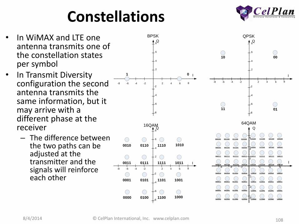
8/4/2014 © CelPlan International, Inc. www.celplan.com 108
Constellations • In WiMAX and LTE one
antenna transmits one of the constellation states per symbol
• In Transmit Diversity configuration the second antenna transmits the same information, but it may arrive with a different phase at the receiver – The difference between
the two paths can be adjusted at the transmitter and the signals will reinforce each other
Q
2-2 4 6 8-4-6-8
2
4
6
8
-2
-4
-6
-8
1010111001100010
0011 0111 1111 1011
0001 0101 1101 1001
1000110001000000
I
Q
2-2 4 6-4-6
2
4
6
-2
-4
-6
000100 001100 011100 010100
000101 001101 011101 010101
000111 001111 011111 010111
000110 001110 011110 010110
000010 001010 011010 010010
000011 001011 011011 010011
000001 001001 011001 010001
000000 001000 011000 010000
110010 111010 101010 100010
110011 111011 101011 100011
110001 111001 101001 100001
110000 111000 101000 100000
110100 111100 101100 100100
110101 111101 101101 100101
110111 111111 101111 100111
110110 111110 101110 100110I
Q
2-2 4 6 8-4-6-8
2
4
6
8
-2
-4
-6
-8
01 I
Q
2-2 4 6 8-4-6-8
2
4
6
8
-2
-4
-6
-8
00
0111
10
I
BPSK QPSK
16QAM64QAM
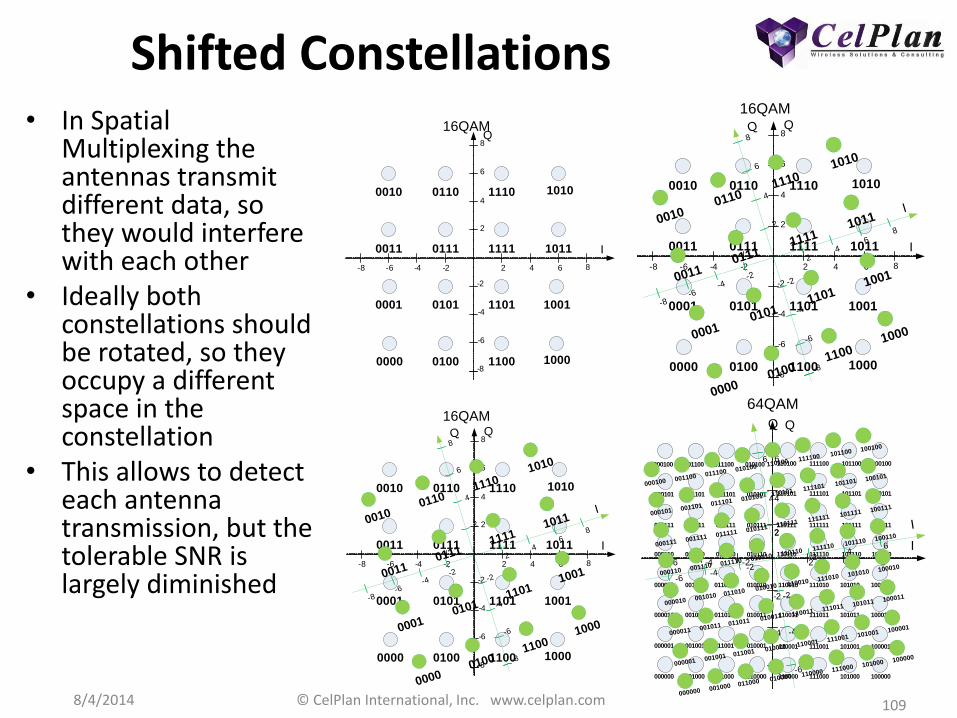
8/4/2014 © CelPlan International, Inc. www.celplan.com 109
Shifted Constellations • In Spatial
Multiplexing the antennas transmit different data, so they would interfere with each other
• Ideally both constellations should be rotated, so they occupy a different space in the constellation
• This allows to detect each antenna transmission, but the tolerable SNR is largely diminished
Q
2-2 4 6 8-4-6-8
2
4
6
8
-2
-4
-6
-8
1010111001100010
0011 0111 1111 1011
0001 0101 1101 1001
1000110001000000
I
Q
2
-2
46
8
-4-6
-8
2
4
6
8
-2
-4
-6
-8
1010
1110
0110
0010
00110111
11111011
00010101
11011001
1000
1100
0100
0000
I
16QAM
Q
2-2 4 6-4-6
2
4
6
-2
-4
-6
000100 001100 011100 010100
000101 001101 011101 010101
000111 001111 011111 010111
000110 001110 011110 010110
000010 001010 011010 010010
000011 001011 011011 010011
000001 001001 011001 010001
000000 001000 011000 010000
110010 111010 101010 100010
110011 111011 101011 100011
110001 111001 101001 100001
110000 111000 101000 100000
110100 111100 101100 100100
110101 111101 101101 100101
110111 111111 101111 100111
110110 111110 101110 100110I
Q
2
-2
46
-4-6
2
4
6
-2
-4
-6
000100 001100 011100 010100
000101 001101 011101 010101
000111 001111 011111 010111
000110 001110 011110 010110
000010 001010 011010 010010
000011 001011 011011 010011
000001 001001 011001 010001
000000 001000 011000 010000
110010 111010 101010 100010
110011 111011 101011 100011
110001 111001 101001 100001
110000 111000 101000 100000
110100 111100 101100 100100
110101 111101 101101 100101
110111 111111 101111 100111
110110 111110 101110 100110
I
64QAM
Q
2-2 4 6 8-4-6-8
2
4
6
8
-2
-4
-6
-8
1010111001100010
0011 0111 1111 1011
0001 0101 1101 1001
1000110001000000
I
Q
2-2 4 6 8-4-6-8
2
4
6
8
-2
-4
-6
-8
1010111001100010
0011 0111 1111 1011
0001 0101 1101 1001
1000110001000000
I
Q
2
-2
46
8
-4-6
-8
2
4
6
8
-2
-4
-6
-8
1010
1110
0110
0010
00110111
11111011
00010101
11011001
1000
1100
0100
0000
I
16QAM
16QAM

8/4/2014 © CelPlan International, Inc. www.celplan.com 110
MIMO Configurations • The Maximum Likelihood Detector (MLD) has to consider possible combinations of s0
and s1, which could be a large number • For two symbols the total number of combinations for 64QAM, 16QAM and QPSK is
4,368 • This number can be reduced to 1,092 combinations if a quadrant approach is used.
– In this approach, instead of checking all possible combinations, quadrants are tested first, eliminating the rejected quadrant combinations
𝐷𝟐(𝑠0, 𝑠1) = 𝑟0 − ℎ00𝑠0 − ℎ𝟏𝟎𝑠𝟏2 + 𝑟1 − ℎ𝟎𝟏𝑠0 − ℎ11𝑠1
2 Maximum Likelihood Detector
Number of RX antennas
Number of TX antennas 1 2 3 4
1 Baseline Downlink: MRC
Uplink: Collaborative MIMO MRC MRC
2 STC (Matrix A) 2xSMX (Matrix B)
STC+ 2xMRC (Matrix A) 2xSMX (Matrix B)
STC+3xMRC (Matrix A) STC+
4xMRC (Matrix A)
4 STC (Matrix A) 2xSMX (Matrix B)
STC+ 2xMRC (Matrix A) 2xSMX (Matrix B)
STC+3xMRC (Matrix A) 4xSMX (Matrix C)
• The table below shows the best combinations for the various numbers of antennas
8/4/2014 © CelPlan International, Inc. www.celplan.com 111
Adaptive MIMO Switching (AMS)
• Transmit Diversity presents a higher throughput than Spatial Multiplexing at low SNIR levels, whereas Spatial Multiplexing results in a higher throughput than Transmit diversity for high SNIR levels
• AMS automatically chooses the solution that gives the best throughput at each location
8/4/2014 © CelPlan International, Inc. www.celplan.com 112
5.5 Multi-user MIMO
Uplink MIMO
Multi-user MIMO
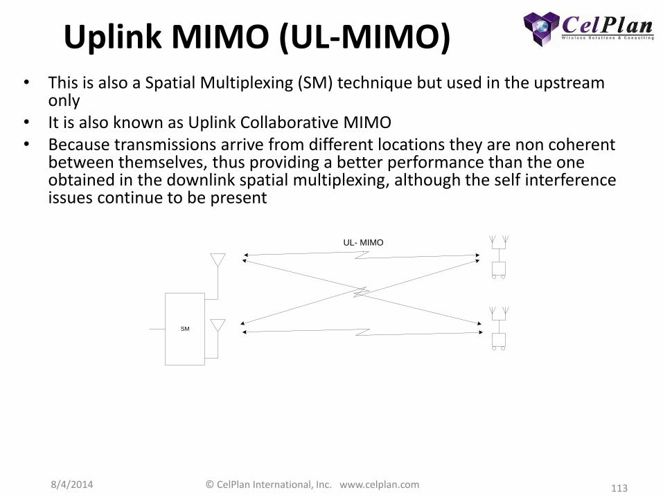
8/4/2014 © CelPlan International, Inc. www.celplan.com 113
Uplink MIMO (UL-MIMO) • This is also a Spatial Multiplexing (SM) technique but used in the upstream
only • It is also known as Uplink Collaborative MIMO • Because transmissions arrive from different locations they are non coherent
between themselves, thus providing a better performance than the one obtained in the downlink spatial multiplexing, although the self interference issues continue to be present
SM
UL- MIMO
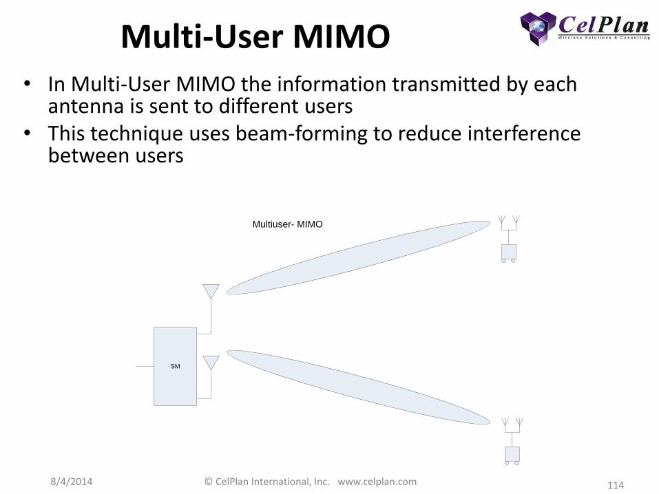
8/4/2014 © CelPlan International, Inc. www.celplan.com 114
Multi-User MIMO • In Multi-User MIMO the information transmitted by each
antenna is sent to different users • This technique uses beam-forming to reduce interference
between users
SM
Multiuser- MIMO

8/4/2014 © CelPlan International, Inc. www.celplan.com 115
6. Antenna Correlation

8/4/2014 © CelPlan International, Inc. www.celplan.com 116
Antenna Correlation • Multiple antenna systems are said to have correlated antennas
if the signals received by the receive antennas are coherent, i.e. are similar to each other
• When the received signals are differentiated (non-coherent) the antennas are said to be uncorrelated
• Channel (H) between two transmit and receive antennas is represented by four virtual connections (hnn) for each delayed path – The matrix that defines the virtual connections of each
delayed complex channel path is given below
• The correlation between antennas is a function of the local scattering and is a function of the Angular Spread (AS), Angle of Arrival (AoA) and Direction of Travel (DoT) – This correlation is not constant, varying significantly over a
geographical area
• The correlation between antennas can be expressed in terms of signal (ρ) observed at each antenna element
• ITU Advanced Antenna Models replace 𝑅𝑡𝑥 by 𝑅𝑒𝑁𝐵 , 𝜌𝑡𝑥 by 𝛼 and 𝜌𝑟𝑥 by 𝛽
• The 𝛼 and 𝛽 values represent the different channel types and range from 0 to 1
TX1
TX2
RX1
RX2
h11
h22
h12
h21
𝑯 =ℎ11 ℎ12ℎ21 ℎ22
Matrix H of a complex channel path
𝒓 =𝑟1𝑟2=ℎ11 ℎ12ℎ21 ℎ22
𝑥1𝑥2 +𝑛1𝑛2
Output complex signal for a single delayed path
𝜌 =𝐸(ℎ11ℎ12
∗)
𝐸(ℎ11ℎ11∗) 𝐸(ℎ12ℎ12
∗) Output complex signal for a single
delayed path
𝐸 ℎ11ℎ11∗ = 1 Expectancy normalization
𝜌𝑡𝑥 = 𝐸 ℎ11ℎ12∗
Correlation between transmit antennas as measured at antenna 1
𝜌𝑟𝑥 = 𝐸 ℎ22ℎ12∗
Correlation between receive antennas as measured at antenna 2
𝑅 = 𝑅𝑡𝑥⨂𝑅𝑟𝑥 Correlation matrix
𝑅𝑡𝑥 =1 𝜌𝑡𝑥𝜌𝑡𝑥∗ 1
Transmit correlation matrix
𝑅𝑟𝑥 =1 𝜌𝑟𝑥𝜌𝑟𝑥∗ 1
Receive correlation matrix
𝑅𝑒𝑁𝐵 =1 𝛼𝛼∗ 1
𝑅𝑈𝐸 =1 𝛽𝛽∗ 1
eNB and UE Antenna correlation
𝑅𝑠𝑝𝑎𝑡𝑖𝑎𝑙 = 𝑅𝑒𝑁𝐵⨂𝑅𝑈𝐸 =1 ∝∝∗ 1
⨂1 𝛽𝛽∗ 1
=
=
1𝛽∗
𝛽1
𝛼𝛼𝛽∗
𝛼∗ 𝛼∗𝛽 1𝛼∗𝛽∗ 𝛼∗ 𝛽∗
𝛼𝛽𝛼𝛽1
Spatial antenna correlation
Low
correlation Medium
correlation High
correlation
α 0 0.3 0.9
β 0 0.9 0.9
0.5 λ1.5 λ
eNB UE eNB UE
High Correlation Medium Correlation
Cross Polarized antennas
8/4/2014 © CelPlan International, Inc. www.celplan.com 117
Correlation • The correlation coefficient, denoted by r tells us how closely data in a
scatterplot fall along a straight line • The closer that the absolute value of r is to one, the closer that the data are
described by a linear equation • Data with values of r close to zero show little to no straight-line relationship
• The data we are working with are paired data, each pair of which will be denoted
by (xi,yi) – Calculate x, the mean of all of the first coordinates of the data xi – Calculate y, the mean of all of the second coordinates of the data yi – Calculate s x the sample standard deviation of all of the first coordinates of the data xi – Calculate s y the sample standard deviation of all of the second coordinates of the data yi
• Use the formula (zx)i = (xi – x) / s x and calculate a standardized value for each xi • Use the formula (zy)i = (yi – y) / s y and calculate a standardized value for each yi • Multiply corresponding standardized values: (zx)i(zy)i • Add the products from the last step together • Divide the sum from the previous step by n – 1, where n is the total number of
points in our set of paired data – The result of all of this is the correlation coefficient r
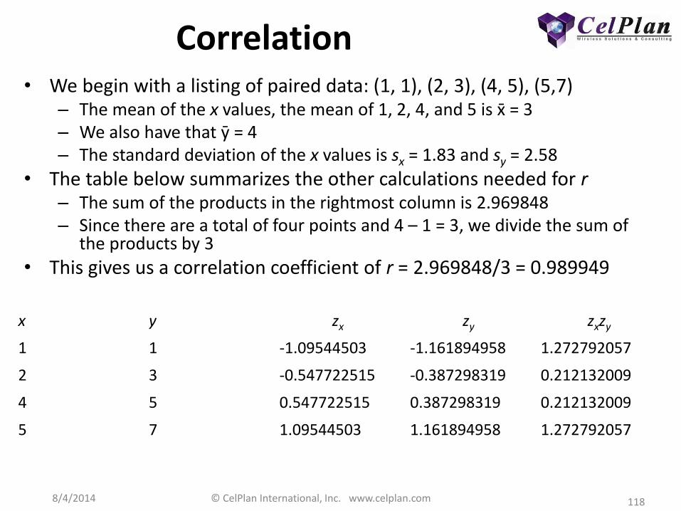
8/4/2014 © CelPlan International, Inc. www.celplan.com 118
Correlation • We begin with a listing of paired data: (1, 1), (2, 3), (4, 5), (5,7)
– The mean of the x values, the mean of 1, 2, 4, and 5 is x = 3 – We also have that y = 4 – The standard deviation of the x values is sx = 1.83 and sy = 2.58
• The table below summarizes the other calculations needed for r – The sum of the products in the rightmost column is 2.969848 – Since there are a total of four points and 4 – 1 = 3, we divide the sum of
the products by 3
• This gives us a correlation coefficient of r = 2.969848/3 = 0.989949 x y zx zy zxzy
1 1 -1.09544503 -1.161894958 1.272792057
2 3 -0.547722515 -0.387298319 0.212132009
4 5 0.547722515 0.387298319 0.212132009
5 7 1.09544503 1.161894958 1.272792057
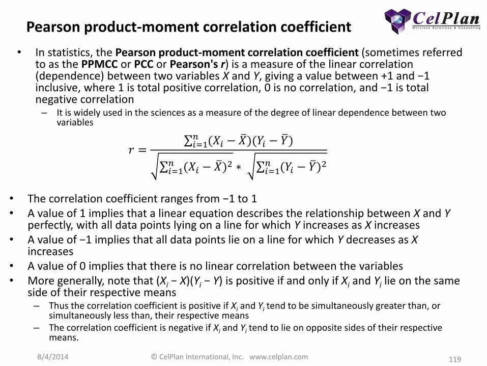
8/4/2014 © CelPlan International, Inc. www.celplan.com 119
Pearson product-moment correlation coefficient
• In statistics, the Pearson product-moment correlation coefficient (sometimes referred to as the PPMCC or PCC or Pearson's r) is a measure of the linear correlation (dependence) between two variables X and Y, giving a value between +1 and −1 inclusive, where 1 is total positive correlation, 0 is no correlation, and −1 is total negative correlation – It is widely used in the sciences as a measure of the degree of linear dependence between two
variables
𝑟 = (𝑋𝑖 − 𝑋 )(𝑌𝑖 − 𝑌 )𝑛𝑖=1
(𝑋𝑖 − 𝑋 )2𝑛
𝑖=1 ∗ (𝑌𝑖 − 𝑌 )2𝑛
𝑖=1
• The correlation coefficient ranges from −1 to 1 • A value of 1 implies that a linear equation describes the relationship between X and Y
perfectly, with all data points lying on a line for which Y increases as X increases • A value of −1 implies that all data points lie on a line for which Y decreases as X
increases • A value of 0 implies that there is no linear correlation between the variables • More generally, note that (Xi − X)(Yi − Y) is positive if and only if Xi and Yi lie on the same
side of their respective means – Thus the correlation coefficient is positive if Xi and Yi tend to be simultaneously greater than, or
simultaneously less than, their respective means – The correlation coefficient is negative if Xi and Yi tend to lie on opposite sides of their respective
means.

8/4/2014 © CelPlan International, Inc. www.celplan.com 120
Antenna Correlation • Variance is a measure of the variability or spread in a set of data
– Mathematically, it is the average squared deviation from the mean score
• 𝑉𝑎𝑟 𝑋 = (𝑋𝑖 − 𝑋)2 𝑁 =
𝑥𝑖2
𝑁 𝑁
𝑖=0 𝑁𝑖=0
N is the number of scores in a set of scores X is the mean of the N scores. Xi is the ith raw score in the set of scores xi is the ith deviation score in the set of scores Var (X) is the variance of all the scores in the set
• Covariance is a measure of the extent to which corresponding elements from two sets of ordered data move in the same direction
• 𝑉𝑎𝑟 𝑋 = (𝑋𝑖−𝑋)(𝑌𝑖 − 𝑌) 𝑁 = 𝑥𝑖𝑦𝑖𝑁
𝑁𝑖=0 𝑁
𝑖=0 N is the number of scores in each set of data X is the mean of the N scores in the first data set Xi is the ith raw score in the first set of scores xi is the ith deviation score in the first set of scores Y is the mean of the N scores in the second data set Yi is the ith raw score in the second set of scores yi is the ith deviation score in the second set of scores Cov (X, Y) is the covariance of corresponding scores in the two sets of data
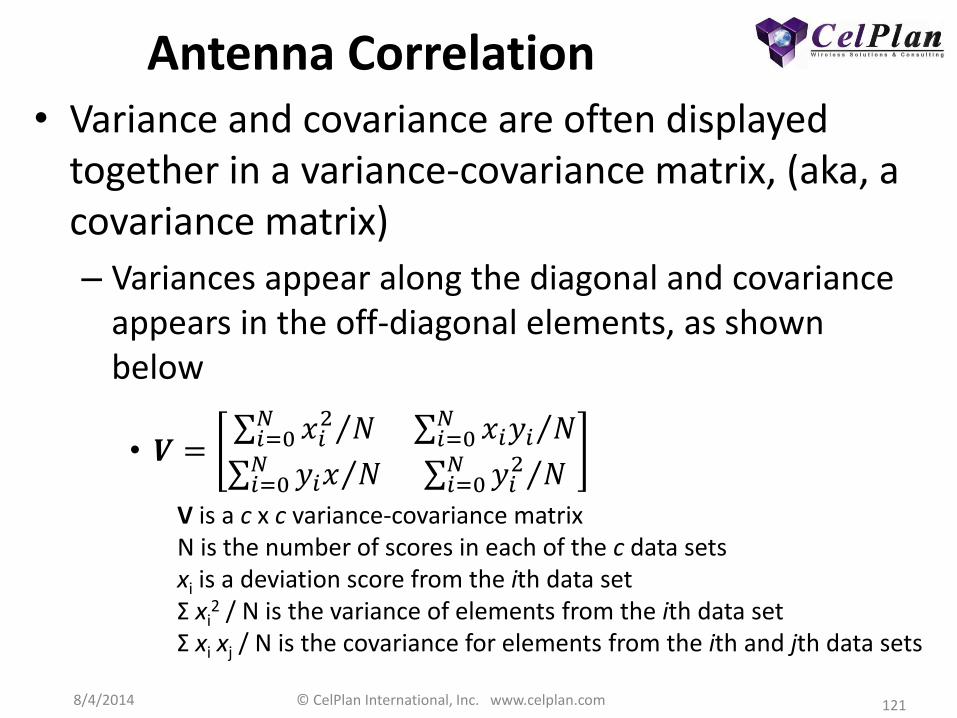
8/4/2014 © CelPlan International, Inc. www.celplan.com 121
Antenna Correlation • Variance and covariance are often displayed
together in a variance-covariance matrix, (aka, a covariance matrix)
– Variances appear along the diagonal and covariance appears in the off-diagonal elements, as shown below
• 𝑽 = 𝑥𝑖
2 𝑁 𝑁𝑖=0 𝑥𝑖𝑦𝑖 𝑁
𝑁𝑖=0
𝑦𝑖𝑥 𝑁 𝑁𝑖=0 𝑦𝑖
2 𝑁 𝑁𝑖=0
V is a c x c variance-covariance matrix N is the number of scores in each of the c data sets xi is a deviation score from the ith data set Σ xi
2 / N is the variance of elements from the ith data set Σ xi xj / N is the covariance for elements from the ith and jth data sets

8/4/2014 © CelPlan International, Inc. www.celplan.com 122
Correlation Matrix • Correlation Matrix is a quantity closely related to
the covariance matrix is the correlation matrix, the matrix of Pearson product-moment correlation coefficients between each of the random variables in the random vector , which can be written
• 𝑐𝑜𝑟𝑟 𝑋 = (𝑑𝑖𝑎𝑔(Σ))−1
2 Σ(𝑑𝑖𝑎𝑔(Σ))−1
2
– 𝑑𝑖𝑎𝑔(Σ) is the matrix of the diagonal elements of Σ (i.e., a diagonal matrix of the variances of 𝑋𝑖for i=1,2,…n
• Equivalently, the correlation matrix can be seen as the covariance matrix of the standardized random variables 𝑋𝑖 𝜎 𝑋𝑖 for i=1,2,…n
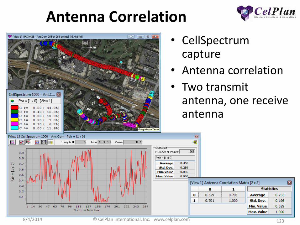
8/4/2014 © CelPlan International, Inc. www.celplan.com 123
Antenna Correlation
• CellSpectrum capture
• Antenna correlation
• Two transmit antenna, one receive antenna
8/4/2014 © CelPlan International, Inc. www.celplan.com 124
7. AAS
Antenna Array System (AAS) Advanced Antenna System (AAS) Adaptive Antenna Steering (AAS)
Beamforming
8/4/2014 © CelPlan International, Inc. www.celplan.com 125
Antenna Array System (AAS) Advanced Antenna System (AAS)
or Adaptive Antenna Steering (AAS) or Beamforming
• Advanced antenna systems can be built by multiple elements which are fed with different signal phases and can generate nulls and poles at certain directions
• This feature is used to reinforce signals and cancel interferences • Two of the main methods, direction of arrival and antenna steering, are
described next • Direction of Arrival (DoA) beamforming is done by detecting the direction
with which the signal and interferers arrive, reinforcing the first one and canceling the others
• The maximum number of cancelled signal is equal to the number of antenna elements minus one
• The re-enforcement is usually of the order of few dB and the canceling is not complete either
• As different implementations have large variations, these parameters have to be specified at design time based on the equipment used

8/4/2014 © CelPlan International, Inc. www.celplan.com 126
Antenna Steering or Beamforming
• It is used to direct the signal transmission or reception towards the desired signal or away from interferers
• The concept is based on the combination of signals from an array of antennas
• These arrays are also known as smart antennas and the figure illustrates an array (linear) of eight antennas, spaced by a distance d
• Although the array is made of omni antennas it has a directional pattern that can be calculated by adding the signal received from each antenna at a certain distance
d
d
d
d
d
a1
a3
a2
a4
a6
d
a8
d
a5
a7
Sum sin
Sum cos

8/4/2014 © CelPlan International, Inc. www.celplan.com 127
Antenna Steering or Beamforming
• This combination results in the pattern of figure on the left for eight antennas separated by λ/2
• This pattern can be modified by changing the phases of the signals to each antenna, as shown in figure to the right
8/4/2014 © CelPlan International, Inc. www.celplan.com 128
Antenna Steering or Beamforming
• The adaptive beamforming uses the information of symbols received by the array, to define the desired pattern – The signal phases to different antennas are adjusted
dynamically
• The array antennas can be distributed in a line, forming linear arrays, or on a plane, forming planar arrays
• The number of elements in the array defines how many directions can be chosen simultaneously – This number is equal to N-1 directions, where N is the
number of elements in the array – The phases can be adjusted to enhance the reception for
the direction or cancel the signal from it

8/4/2014 © CelPlan International, Inc. www.celplan.com 129
8. MIMO Performance
8/4/2014 © CelPlan International, Inc. www.celplan.com 130
MIMO Performance
• The performance of the different MIMO methods is derived from literature and we display here average values
• The figures show the SNR required for different levels of Bit Error Rate depending on the number of antennas and modulation scheme

8/4/2014 © CelPlan International, Inc. www.celplan.com 131
MIMO Error Probability in a Rayleigh Channel
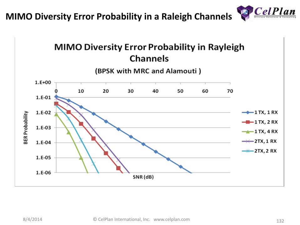
8/4/2014 © CelPlan International, Inc. www.celplan.com 132
MIMO Diversity Error Probability in a Raleigh Channels
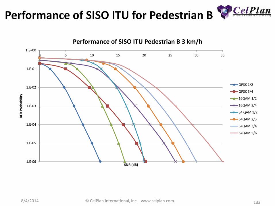
8/4/2014 © CelPlan International, Inc. www.celplan.com 133
Performance of SISO ITU for Pedestrian B
1.E-06
1.E-05
1.E-04
1.E-03
1.E-02
1.E-01
1.E+00
0 5 10 15 20 25 30 35
BER
Pro
bab
ility
SNR (dB)
Performance of SISO ITU Pedestrian B 3 km/h
QPSK 1/2
QPSK 3/4
16QAM 1/2
16QAM 3/4
64 QAM 1/2
64QAM 2/3
64QAM 3/4
64QAM 5/6

8/4/2014 © CelPlan International, Inc. www.celplan.com 134
Performance of MIMO Matrix A
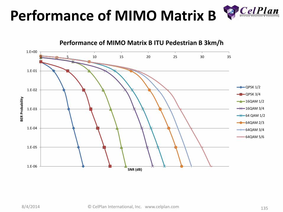
8/4/2014 © CelPlan International, Inc. www.celplan.com 135
Performance of MIMO Matrix B
1.E-06
1.E-05
1.E-04
1.E-03
1.E-02
1.E-01
1.E+00
0 5 10 15 20 25 30 35
BER
Pro
bab
ility
SNR (dB)
Performance of MIMO Matrix B ITU Pedestrian B 3km/h
QPSK 1/2
QPSK 3/4
16QAM 1/2
16QAM 3/4
64 QAM 1/2
64QAM 2/3
64QAM 3/4
64QAM 5/6
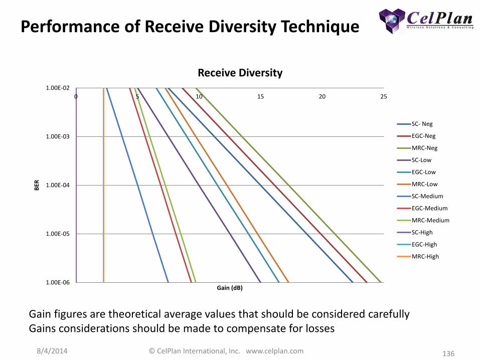
8/4/2014 © CelPlan International, Inc. www.celplan.com 136
Performance of Receive Diversity Technique
1.00E-06
1.00E-05
1.00E-04
1.00E-03
1.00E-02
0 5 10 15 20 25
BER
Gain (dB)
Receive Diversity
SC- Neg
EGC-Neg
MRC-Neg
SC-Low
EGC-Low
MRC-Low
SC-Medium
EGC-Medium
MRC-Medium
SC-High
EGC-High
MRC-High
Gain figures are theoretical average values that should be considered carefully Gains considerations should be made to compensate for losses

8/4/2014 © CelPlan International, Inc. www.celplan.com 137
Performance of Transmit Diversity Technique
Gain figures are theoretical average values that should be considered carefully Gains considerations should be made to compensate for losses
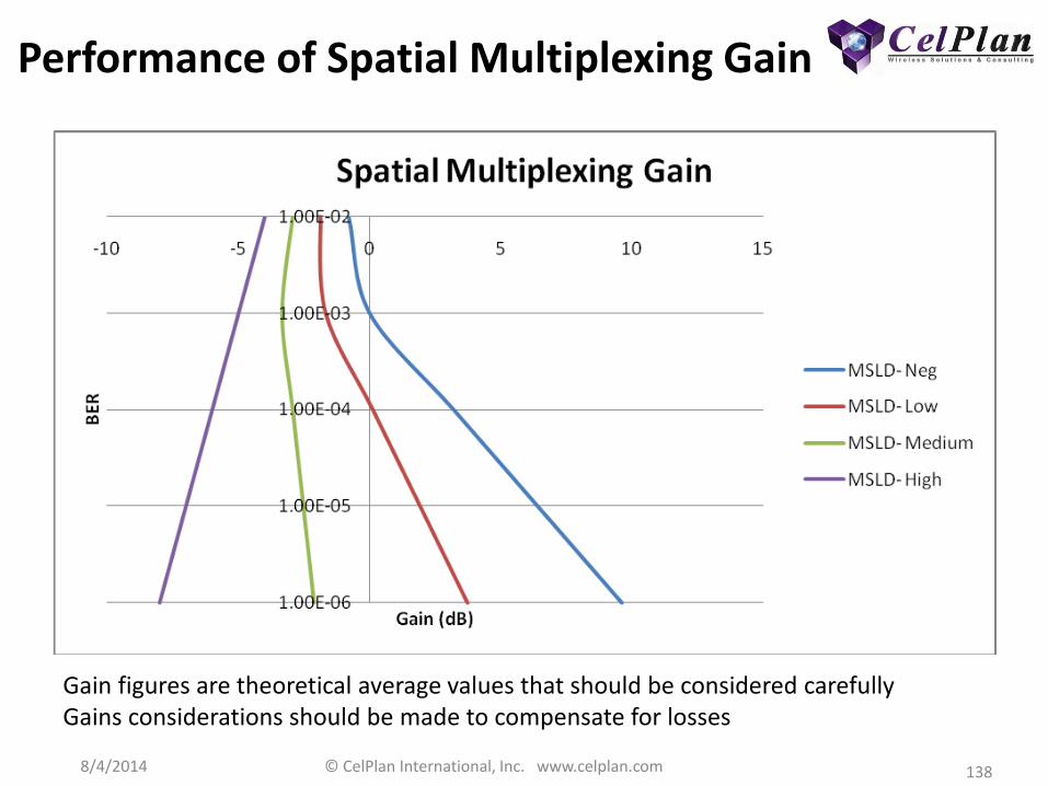
8/4/2014 © CelPlan International, Inc. www.celplan.com 138
Performance of Spatial Multiplexing Gain
Gain figures are theoretical average values that should be considered carefully Gains considerations should be made to compensate for losses
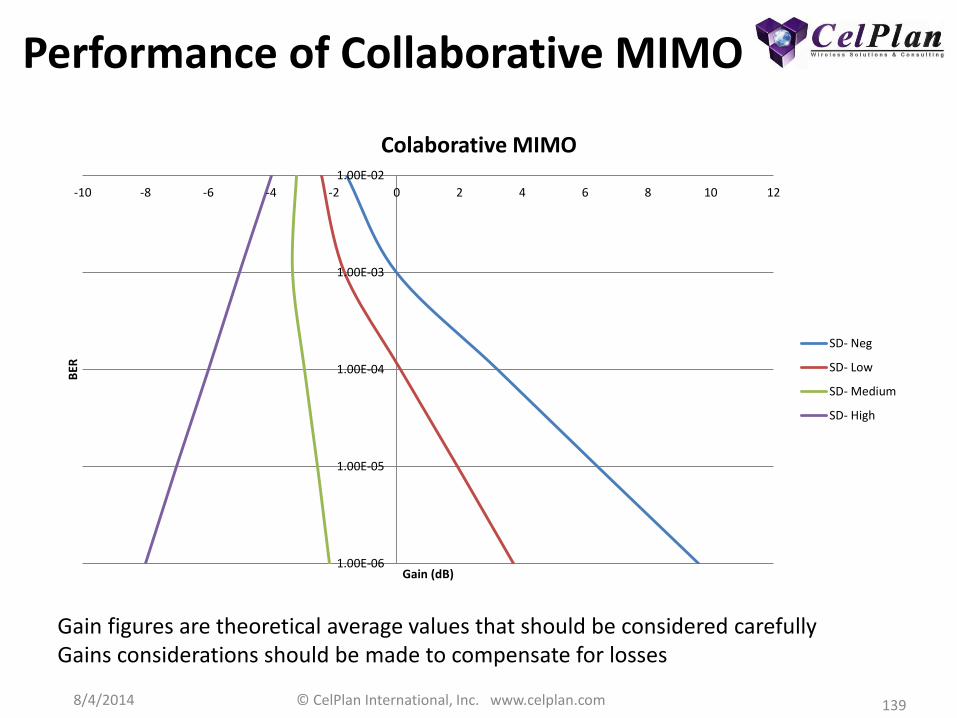
8/4/2014 © CelPlan International, Inc. www.celplan.com 139
Performance of Collaborative MIMO
1.00E-06
1.00E-05
1.00E-04
1.00E-03
1.00E-02
-10 -8 -6 -4 -2 0 2 4 6 8 10 12
BER
Gain (dB)
Colaborative MIMO
SD- Neg
SD- Low
SD- Medium
SD- High
Gain figures are theoretical average values that should be considered carefully Gains considerations should be made to compensate for losses

8/4/2014 © CelPlan International, Inc. www.celplan.com 140
9. CelPlan New Products
CellSpectrum
CellDesigner

8/4/2014 © CelPlan International, Inc. www.celplan.com 141
9.1 CellDesigner
A new Generation of Planning Tools
A collaborative work with operators
Your input is valuable
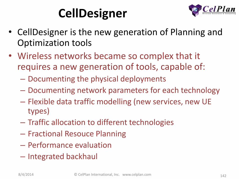
8/4/2014 © CelPlan International, Inc. www.celplan.com 142
CellDesigner
• CellDesigner is the new generation of Planning and Optimization tools
• Wireless networks became so complex that it requires a new generation of tools, capable of: – Documenting the physical deployments
– Documenting network parameters for each technology
– Flexible data traffic modelling (new services, new UE types)
– Traffic allocation to different technologies
– Fractional Resouce Planning
– Performance evaluation
– Integrated backhaul

All information contained in this document is property of CelPlan Technologies. Unauthorized copies are prohibited.
CellDesigner™ Simultaneous Multi-Technology Support
• Supports all wireless technology standards: – LTE–A (TDD and FDD), WiMAX, WI-FI,
WCDMA (UMTS), HSPA, HSPA+, IS2000 (1xRTT, EVDO), GSM (including Frequency Hoping), GPRS, EDGE, EDGE-E, CDMA One, PMR/LMR (Tetra and P25), MMDS/LMDS, DVB-T/H, and Wireless Backhaul
• Full network representation – Site, Tower, Antenna Housing, Antenna
System, Sector, Cell, Radio
– Full network parameter integration
– KPI integration
• Full implementation of the Korowajczuk 3D model, capable of performing simultaneously outdoor and indoor multi-floor predictions
• Multi-technology dynamic traffic simulation
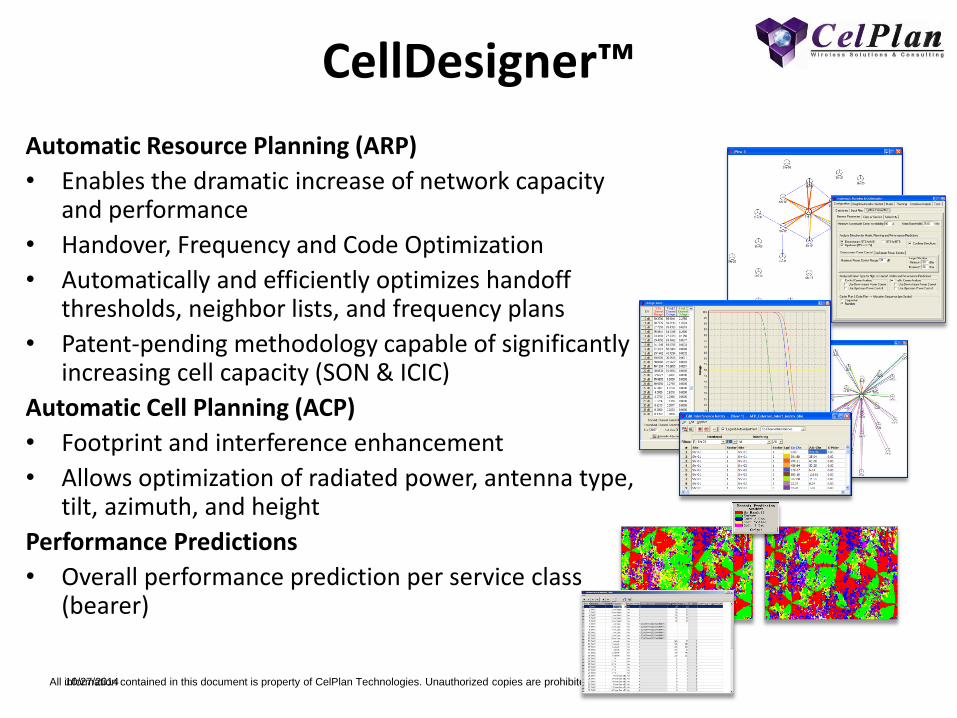
All information contained in this document is property of CelPlan Technologies. Unauthorized copies are prohibited.
CellDesigner™
Automatic Resource Planning (ARP)
• Enables the dramatic increase of network capacity and performance
• Handover, Frequency and Code Optimization
• Automatically and efficiently optimizes handoff thresholds, neighbor lists, and frequency plans
• Patent-pending methodology capable of significantly increasing cell capacity (SON & ICIC)
Automatic Cell Planning (ACP)
• Footprint and interference enhancement
• Allows optimization of radiated power, antenna type, tilt, azimuth, and height
Performance Predictions
• Overall performance prediction per service class (bearer)
10/27/2014

All information contained in this document is property of CelPlan Technologies. Unauthorized copies are prohibited.
CellDesigner™
10/27/2014
Google Earth Integration
• Capable of presenting predictions and measurements live in Google Earth’s 3D environment
Network Master Plan (NMP)
• Patent-pending methodology that simplifies SON and ICIC
Integration of Field Measurement Data
• Collection of data from virtually any type of measurement equipment and any format
• Automatic extraction of propagation parameters
Integration of KPIs
• Comparison reports between reported and calculated KPIS
All information contained in this document is property of CelPlan Technologies. Unauthorized copies are prohibited. 10/27/2014
CellDesigner™
GIS Database Editor
• Allows the editing and processing of geographical databases
Backhaul Planning
• Calculates network interconnections, interference analysis & reporting for point-to-point, microwave transmission links
• Can display obstruction in Fresnel zones as well as the path loss
• Calculates attenuation caused by diffraction.
• Calculates rain attenuation for each link
• Provides link performance and compares against the requirements established by ITU-R

8/4/2014 © CelPlan International, Inc. www.celplan.com 147
Thank You!
Questions?
Leonhard Korowajczuk
www.celplan.com