Embed Size (px)
Citation preview

7 AD-fl46 030 ANALYSIS AND DESIGN METHODOLOGY FOR VLSI COMPUTING 1/2.
NETkIORKS(U) INTEGRATED SYSTEMS INC PALO ALTO CAH LEV-ARI AUG 84 ISI-46 N000i4-83-C-0377p UNCLASSIFIED F/G 9/2 NL

I ---- --; -122 ------
I"D
1.0.
11111 1.25 1 1. I.6,__. !11
MICROCOPY RESOLUTION' TEST CHARTNATIONAL BUREAU OF STANDARDS- 1963-A
:2 " -- . .. - _- - . . - - : I.

AD-A146 030
ANALYSIS AND DESIGN METHODOLOGY FORVLSI COMPUTING NETWORKS 0
FINAL REPORT
HANOCH LEV-ARI
PREPARED FOR:
OFFICE OF NAVAL RESEARCH
800 NORTH QUINCY STREET
ARLINGTON, VIRGINIA 22217
ATTENTION: DR. DAVID W. MIZELL
PREPARED UNDER: DTICCONTRACT NO. N00014-83-C-0377 ELECTE
SSEP26
DSTM1UTON ST4TMEITA~jippvedfixpublic releau"Distribution Unlimited i
ISI REPORT 46 * AUGUST 1984 -9
I1N1 FILE COPY101 Universily Avenue Palo Alto, CA 94301-1695 Telephone 415'853-8400
84 09 05o1

TABLE OF CON T Ts
Section Title Pale 0
1 INTRODUCTION ........... ...................... 12 MODELING PARALLEL ALGORITHMS AND ARCHITECTURES ..... 5
2.1 Toward a Formal Definition of Algorithms
and Architectures ........ ................. 5
2.2 Modular Computing Networks ...... ............ 8
2.3 Causality and Executions .... ............. .. 16
2.4 Hierarchical Composition of MCNs ......... 19
2.5 Comparison of MCNs with Other Network Models . . . 23
2.5.1 Block-Diagrams and Finite-State Machines . 23
2.5.2 Data-Flow-Graphs and Petri-Nets . . . . 25
2.5.3 High-Level Programming Languages ....... .27
2.5.4 Summary ....... .................. . 28 e2.6 Formal Language Representation of MCqs ....... .28
2.7 Summary ...................... 32
3 STRUCTURAL ANALYSIS OFMs . . . . . . . ....... 35
3.1 Numbering of Variables and Processors .. . . . . 35..
3.2 Dimensionality and Order .... .......... . . 36
3.3 Schedules. Delay and Throughput ........... . 40
3.4 Space-Time Diagrams ...... ................ .47
3.5 Summary . . . . ... . . . . . . ... . .. . . . 56
4 ITERATIVE AND COMPLETELY REGULAR NETWORKS ... ....... 57
4.1 Iterative MCNs and Hardware Architectures . . . .. 57
4.2 Completely Regular MlCs ..... .............. . 67
4.2.1 Space-Time Representations in Z3 ..... 68
4.2.2 Spatial Projection of MCNs in ..... 70
4.3 Modular Decomposition of CN Models .. ........ . 72
4.3.1 Modular Decomposition of Linear
Multivariable Filters .... ........... 73 - .
.f •.

S CLASSIFICATION OF ARCHITECTURES ............ 79
5.1 Topological Equivalence .............. 81
5.2 Architectural Equivalence .... ............. ... 85
5.3 Periodicity Analysis and Throughput .. ........ . 85
5.4 Boundary Analysis ................. 88
5.5 Summary ...................... 92
6 CLASSIFICATION OF SPACE-TIME REPRESENTATIONS ...... . 95...-
6.1 The Fundamental Space-Time Configurations ..... ... 95
6.2 Architectures with Local Memory . ......... 96
6.3 Boundary Analysis ....... ................. .101
6.3.1 The Configurations LM1, L2, R2 ......... 101
6.3.2 The Configurations RM2, 13, B3a, H3b . . . 104
6.3.3 The Configurations HM3a, R4 ........ 105
6.3.4 Summary ..... ............ . . . ... 105
6.4 Interleaving Architectures by Local Memory . ... 105
6.5 Summary............... . ...... 107
7 CONCLUSIONS ...................... 109
8 TECHNICAL PUBLICATIONS ...................... .111
REF1ERENCES ................................... 113 .O -
APPENDIX A: PROOF OF THEOREM 2.2 FOR INFINITE MCNs ...... 117
APPENDIX B: ADMISSIBLE ARCHITECTURES . . . ........... 119
APPENDIX C: PROOF OF THEOREM 2.3, MINIMAL EXECUTIONS OF
FINITE MCNs . . . . . ............... 121
APPENDIX D: ELEMENTARY EQUIVALENCE TRANSFORMATIONS ....... 127
APPENDIX E: ANALYSIS OF MATRIX MULTIPLIERS .............. 129
APPENDIX F: EQUIVALENCE VIA LINEAR TRANSFORMATIONS . . . . . . . 141
cesson For' rA&I
_J but ont -
Av,41.ibfljty Codes
A-, v a I _ o r..' t I Special .

r
SECTION 1
INTRODUaION
Several methods for modeling and analysis of parallel algorithms and
architectures have been proposed in the recent years. These include
recursion-type methods, like recursion equations, z-transform descriptions
and 'do-loops' in high-level programming languages, and precedence-graph-
type methods like data-flow graphs (marked graphs) and related Petri-net
derived models [1], [2]. Most efforts have been recently directed towards
developing methodologies for structured parallel algorithms and
architectures and, in particul'ar, for systolic-array-like systems [3J-[10]. PSome important properties of parallel algorithms have been identified in the
process of this research effort. These include executability (the absence
of deadlocks) pipelinability, regularity of structure, locality of
interconnections, and dimensionality. The research has also demonstrated
the feasibility of multirate systolic arrays with different rates of data
propagation along different directions in the array.
In this final report we present ,a new methodolo y for modeling and
! analysis of parallel algorithms and architectures. Our methodology provides
a unified conceptual framework, which-we call modular computina network,
that clearly displays the key properties of parallel systems. In
particular,
(1) Executability of algorithms is easily verified.
(2) Schedules of execution are easily determined. This allows forsimple evaluation of throughput rates and execution delays.
(3) Both synchronous and asynchronous (self-timed) modes of executioncan be handled with the same techniques.
(4) Algorithms are directly mappable into architectures. No elaboratehardware compilation is required.
(5) The description of a parallel algorithm is independent of itsimplementation. All possible choices of hardware implementationare evident from the description of a given algorithm. The

equivalence of existing implementations can be readilydemonstrated.
(6) Both regular and irregular algorithms can be modeled. Models of -regular algorithms are significantly simpler to analyze, sincethey inherit the regularity of the underlying problem.
Our methodology is largely based upon the theory of directed graphs and can,
therefore, be expressed both informally, in pictorial fashion, and formally,
in the language of precedence relations and composition of functions. This
duality will, hopefully, help to bridge the gap between the two schools of "
research in this field. An outline of a formal language representation for
modular computing networks is also provided. ,
The multiplicity of possible hardware implementations for a given
computational scheme is efficiently displayed by a space-time
representation, a notational tool that has been incorporated into some
recent methodologies for modeling, analysis and design of parallel
architectures [23-31). Coordinate transformations of a given space-time
representation produce distinct hardware configurations which are equivalent
in the sense of being the implementations of the same computational scheme.
The problem of mapping a given algorithm into a desired hardware
configuration can, therefore, be partly reduced to choosing the appropriate
coordinate transformation in space-time. In particular, uniform recurrence
relations, which correspond to systolic-array architectures, are described
by regular apace-time representations. This implies that only linear
coordinate transformations are required, and that the entire computational
scheme can be described by a small collection of vectors in space-time, the
devendence vectors [25,27,28,30]. Consequently, the selection of a desired
hardware architecture for a given algorithm reduces to the determination of
an appropriate nonsingular matrix with integer entries. . -
A simple technique for transforming a given 3-dimensional space-time
representation into an equivalent canonical form is presented in Sections 5-
6. A catalogue of canonical forms is constructed, showing a total of 34
distinct systolic architectures. The task of selecting an appropriate
transformation for a given space-time representation reduces, therefore, to
the determination of the equivalent canonical form. The important result,
which has been overlooked in previous research, is that the canonical - -
equivalent of any given space-time representation is unigue. This means
2

that once a space-time representation has been specified there is no
flexibility left in the process of mapping it into systolic-array
architectures.
A small fraction of space-time representation does allow some
flexibility in selecting the hardware architecture, but only at the cost of
inefficient implementation. The well-known example of matrix
multiplication, which has four distinct realizations (see [4,5,7,101) turns
out to be one of the few cases where such flexibility is available. A
closer examination of the structure of the matrices to be multiplied reveals
that each realization is efficient under a different set of structural
assumptions (see Section 6.3). Thus, in summary, carefully specified
algorithms lead to unique space-time representations which, in turn, lead to
essentially unique architectures.
3

p
p
7-p
I
a.
-a.
- L.
1-~
-L
4 L I

SECTION 2
MODELING PARALLEL_&GORITHMS AND ARCHITECTURES
The concepts of 'algorithm' and 'architecture,' which have been widely
used for several decades, still seem to defy a formal definition. Books on
computation and algorithms either take these concepts for granted or provide
a sketchy definition using such broad terms as 'precise prescription.'
'computing agent,' 'well-understood instructions,' 'finite effort' and so
forth. The purpose of this section is to provide a simple formal model for
modeling and analysis of (parallel) algorithms and architectures. This
model, which we call modular comuuting network (MCNQ) exhibits all the
properties usually attributed both to algorithms and to hardware
architectures. As a first step toward the formal introduction of this model
we extract in Section 2.1 the main attributes of algorithms from their
characterizations in the literature. This analysis of literature leads to
the conclusion that algorithms can only be defined in a hierarchical manner,
i.e., as well-formed compositions of simpler algorithms, and that the
simplest (non-decomposable algorithms) cannot and need not be defined. The
L building blocks of the theory of algorithms are characterized in terms of
three attributes: Function (what building blocks do), execution time (how
* long they do it), and complexity (what does it cost to use them). These
observations are incorporated into the modular computing network model, as
described in Sections 2.2 - 2.6.
2.1 TOWAID A FORMAL DEFINITION OF ALGORITHMS AND ARCHITECTURES
In this section we attempt to extract the main attributes of algorithms
and architectures from a randomly chosen sample of 'definitions.' Most
characterizations of algorithms are Seared to the notion of sequential
L execution. Nevertheless, we shall see that this underlying assumption is
5

I uiu u~ u' u~ u . . . . . . . . . . . . . . . .--
*6
almost never made ezpliclt. As a result, the attributes of parallel
algorithms are, in fact, included in the available characterizations.
As a typical example consider the following definition. 'The term 6
'algorithm' in mathematics is taken to mean a computational process, carried
out according to a precise prescription and leading from given objects,
which may be permitted to vary, to a sought-for result' [11]. This
definition simply states that an algorithm is a well-defined input-output
map and that its domain contains at least one element, and usually more than
one. However, the term 'computational process' hints that an algorithm is
more than just a well-defined function. Indeed, 'A function is simply a
relationship between the members of one set and those of another. An
algorithm, on the other hand, is a procedure for evaluating a function'
[121.
But how are functions evaluated? We are told that 'this evaluation is
to be carried out by some sort of computing agent, which may be human,
mechanical, electronic, or whatever' [12]. Thus, the emphasis is on
physical realizability (the existence of a 'computing agent') but not on the
actual details of the realization. The first axiom of the theory of
algorithms is, therefore:
There exist basic functions that are physically realizable.
Further efforts to define physical realizability turn out to be quite -
futile. This is recognized by Aho, Hopcroft and Ullman who say, 'each
instruction of an algorithm must have a 'clear meaning' and must be
executable with a 'finite amount of effort.' Now what is clear to one
person may not be clear to another, and it is often difficult to prove
rigorously that an instruction can be carried out in a finite amount of
time' [131. Physical realizability is a matter of technology: What is non-
realizable today may become realizable in a year or two. The theory of
algorithms has to assume the existence of realizable basic input-output maps
but need not be concerned with the details of their implementation.
Therefore, the core of any theory of algorithms is a non-empty collection of
undefined objects, which we shall call processors. These are the 'computing
agents' mentioned above, and they are assumed to have three attributes:
6

(I) Function (an input-output map)
(ii) Complexity measure
(iii) Execution time
A processor is assumed to be capable of evaluating the input-output map in
the specified execution time. The cost of utilizing the processor is*specified by its complexity measure. Notice that the notion of 'effort'
mentioned above is a combination of the processor's complexity and its
execution time.
It is important to draw a distinction between an algorithm and its
description. An algorithm consists of processors (or basic functions),
corresponding to all the functions that need to be evaluated. For instance,
the computation of sin x via the first 100 terms of its MacLaurin series
requires 100 basic functions, one for each term of the truncated series.
The description of the same algorithm in terms of instructions requires only
one instruction, which will be repeated 100 times with varying coefficients.
Since descriptions of algorithms need to be communicated, stored and
implemented, they must be finite, i.e., contain a finite number of
instructions. The algorithm itself, on the other hand, may consist of an
infinite number of processors, and used to process an infinite number of
inputs into an infinite number of outputs. Such are, for instance, most
signal processing algorithms: Their inputs and outputs are time-series
-which may, in principle, be infinitely long. The executability of these
algorithms depends upon their capability to compute any specific output with
finite time and effort, and to use only a finite number of inputs for this
purpose. This observation also sheds a new light on the concept of
'termination,' which is usually overemphasized in definitions of algorithms.
The basic functions comprising an algorithm are interdependent in the
sense that the outputs of one processor may serve as inputs to other
processors. A complete characterization of an algorithm requires,
therefore, to specify both its basic operations and the interconnection
between these operations. The same statement applies, of course, to block-
diagram representations of hardware, to flow-graphs and, in fact, to any
network-type schematic. While algorithms are commonly described in some
L. 7
- ** * 7

formal language, they can also be described in a schematic manner.
Conversely, schematic hardware descriptions can be transformed into formal
language representations. To emphasize this equivalence we shall introduce
the concept of a modular oomuting network (MCN), which exhibits the common
attributes of both algorithms and architectures. Thus, an MCN is a pair
.°.'
where . , the function of the network, is essentially the collection of
basic functions discussed above, and (, the architecture of the network,
is a directed graph describing the interconnections between basic functions.
A detailed definition is provided in Section 2.1.
The concept of modular computing network is hierarchical b- nature.
Basic functions can be themselves characterized as networks c iven more
basic functions. This requires every MCN to have the three damental
attributes of a basic function: Input-output map. complexit a execution
time. Te shall show in the sequel how to uniquely associate such attributes
with modular computing networks. The theory of MCNs is, in short, the
theory of network composition (deducing the properties of a network from its .
components) and network decomposition (characterizing the components and
structure of a network whose composite properties have been specified).
2.2 MODULAR COMPUTING NETWORKS
A modular computing network (3N0) is a system of interconnected
modules. The structural information about the network is conveyed by -
specifying the interconnections between the modules, most conveniently in
the form of a directed graph (Figure 2-1). The functional information about
the network is conveyed by characterizing the information transferred
between modules and the processing of this information as it passes through
the modules.
The structural attributes of an 30N are completely specified by its
architecture, which is an ordered quadruple
Architecture (S. T. A, P) (2.2)
8

2 3
Figure 2-1. The Directed Graph Associated with a Modular Computing Network
9

I
where S.T are sets whose elements are called sources and siJk,
respectively, and A.P are relations between these sets.
The ancestry relation A specifies the connections of sources to 6
sinks. The elements of A. which are called arcs, are ordered source-sink
pairs
a e A =) a = (st). a S. t a T (2.3)
An arc represents a direct transfer of information from source to sink. Two
basic assumptions govern this transfer:
(1) There are no dangling sources. Every source is connected toexactly one sink.
(2) There are no dangling sinks. Every sink is connected to exactly
one source.
These assumptions mean that the three sets S,T,A have an equal number of
elements, and that the ancestry relation A establishes a one-to-one
correspondence between arcs, sources and sinks, viz..
(S,t) a A <-=> s = A(t) <==) t - A-1 () (2.4)
This one-to-one correspondence will permit us to identify in the sequel each Iarc with its associated source and sink, and to eliminate almost all sinks
and sources from the description of network architectures.
The processing relation P specifies the processing of information
extracted from sinks into transformed information, which is re-injected into
sources. The elements of P, which are called processors, are ordered
pairs of non-empty finite sink-source sequences, viz.,
p a p ==> p - (t 1 .t 2 ,...,t ; lt2P,..., n (2.5)
ti • T, ai I S , 1 a. a, <
10I
t10

The input set (tI t 2 .... t ) consists of all the sinks from which the
processor p extracts information. The transformed Information is
distributed among the members of the output set (si t 82 .... , ). The
one-to-one correspondence oetween sources, sinks and arcs allows us to
describe processor inputs and outputs in terms of arcs and to almost
completely eliminate the notion of sources and sinks. The set of input arcs
i oi a processor p is denoted by AI(p), and the set of output arcs from
the same processor is denoted by A0 (p). Each processor is assumed to have
unique inputs and outputs, namely
~Ai(p)C A (q) -
pvq g P, p # q M M A(P) C Ao(q) (2.6)
Similarly, every collection of processors, Q CP. has its uniquelyIL defined inputs and outputs, viz.,
Ai (Q) : U Ai(p)- Ao(p) (2.7a)peQ psQ0
.1 and
Ao(Q) : Ao(p) - (p A(P) (2.7b)peQ peG
-LIn other words, the inputs of Q are those inputs of processors in Q that
* are not connected to outputs of processors in Q. A similar statement holds
for outputs of Q. In particular, A (P). A (P ) are the inputs andi 0
outputs of the entire network.
Network architectures are most conveniently described by a directed
graph that combines together the ancestry relation A and the processing
* relation P into a single block-diagram-like representation (Figure 2-2a).
-- Sources and sinks are denoted by semi-circles, processors by circles and
arcs are, obviously, denoted by arcs. Sources and sinks are paired, and
each processor has its inputs and outputs adjacent to itself. An obvious
reduction in notation (Figure 2-2b) enhances the comprehensibility of the
description. The reduced form is, essentially, a block-diagram
*representation of the network architecture, and can be interpreted as a
directed graph
]1

Si
2)- ti S
S 36
t
4
a. Fall For. Description
p3 tP3 7
b. Reduced Form Description
Figure 2-2. Equivalent Full Form and Reduced Form Descriptions of -2Network Architectures
12

(V. Al (2.8.)
The set of vertices V of this graph is
V ( AP). P. A (2.8b)0
where A (P) are interpreted as the sources corresponding to the input arcs 0
iand A 0 P) are interpreted as the sinks corresponding to the output arcs.
The arcs of the directed graph coincide with the original set of arcs A.
The interpretation of network architectures as directed graphs puts at our
disposal the powerful tools and results of graph theory. Some of these will
be used in the sequel to characterize and analyze the structure of modular
computing networks.
The functional attributes of an 0N4 are completely determined by its
architecture and by specifying the functional attributes of each processor. .
Thus, the function of a network is an ordered pair
4F M F) (2.9)
where X, F are sets whose elements are called variables and mgs,:
respectively.
The elements of X are sets (i.e., domains) and 'assigning a value to
a variable' amounts to choosing a particular element in the domain
corresponding to that variable. There is one variable, 5. associated
with every arc a £ A of the corresponding architecture. Consequently,
there is a one-to-one correspondence between variables, sources, sinks and
arcs. This correspondence makes it possible to refer to the variables
associated with the inputs of a given processor p as the input variables
of p and denote then by I(p). A similar notation, X (p), is used for
the variables associated with the outputs of the processor p.
The elements of F are multivariable maps. There is one map, f *p
associated with every processor p a P of the corresponding architecture. . ,
It maps the input variables of this processor into the corresponding output
variables, viz.,
13

f : (p) -- > X (p) (2.10)P 1 0
which means that each of the output variables is a function of the input I
variables (not necessarily of all the input variables). This establishes a
precedence relation between the inputs and outputs of a given processor,
via.,
x -> y (2.11)
if x s Ai(P). y A 0 (p) and if y is a function of x (and, possibly,
of other input variables). The transitive closure of this relation Is also
a precedence (i.e.. a partial order): We shall say that x precedes zn
if there exists a sequence of variables such that
x - a. - n
in the sense of (2.11). This global precedence will also be denoted by
x* n * The ancestry (141 of a variable x a X is the set of all
variables that precede x, viz.,
a(x) := (z; z a X, z-) x) (2.12)
These are all the variables that have to be known in order to determine the S _
value of x.
Since the function of a network consisting of a ingle processor p is
r M (P) (P), f)-
there is, essentially, no distinction between the function and the Mg of
p. Thus, the input-output map of a single processor may also be called the
function of the processor. The same is not true for a network consisting of
several processors: The input-output map of a network is a single
multivariable map, relating the outputs of the network to its inputs; the
14
. .

function of the network, in contradistinction, is the collection of the
*atomic maps that comprise the network. The analysis Problem for
C computational networks is to determine the network map from its function.
The synthesis problem is to design an NCN (i.e., specify its structure and
function) that realizes a given multivariable Input-output map.
Modular computing networks need not be finite. In fact, most signal
processing algorithms correspond to infinite MCNs. However, the concept of
finite effort, involved in the evaluation of variables, imposes certain
constraints upon infinite networks. First, the number of inputs and outputs
of every processor must be finite. This means that the graph Ir) describing
the architecture is locally finite [15]. Next, every variable must be
computable with finite effort, so it will be required to have a finite
ancestry, viz.,
lazl < - for all x a 1 (2.13)
We shall also assume that the number of connected components of the
architecture , is countable. A modular computing network that satisfies
the three assumptions stated above--local finiteness, finite ancestry and
countable number of connected components--will be called structurally
finite. The following result characterizes the kind of infinity allowed in
such networks.
Theorem21
A structurally finite NQ4 has a countable number of variables and
processors. The following three statements are equivalent:
(1) The number of variables is finite.
(2) The number of output variables is finite.
(3) The number of processors is finite.
15

Proof:
The countability of the variables and processors of a connected network
is a direct consequence of local finiteness (see, e.g., [151). Since each
connected component has a countable number of variables and processors, the
same is obviously true for a countable number of connected components. Thus
the number of variables and processors of a structurally finite MCN must be
countable. As a consequence of local finiteness, a finite number of
processors implies a finite number of variables and vice versa, so (1) and
(3) are equivalent. Clearly (1) implies (2), while (2), via the finite
ancestry condition, implies (1).
2.3 CAUSALITY AND EXECUTIONS .....
The definition of processors in the previous section did not take into
account any constraints imposed by hardware implementation considerations.
the most important among these constraints is the causality property. It
will be henceforth assumed that an output of a processor cannot become
available before the inputs of the same processor that precede this output
became available. In the beginning all variables are unavailable; the
inputs of the network are made available at a given instant, and following
that event, all variables of the network gradually become available. This
temporally ordered process, which we shall call execution, must be
consistent with the urecedence relation between variables induced by the
directed nature of the architecture (. A network that possesses an
execution in which every variable ultimately becomes available is said to be
executable (or 'live' in the terminology of Petri-nets [11. It is clear
that a network containing a cycle cannot be executable since every variable
C- arc) on the cycle can never become available. In order to satisfy the
causality assumption every variable in the cycle must temporally precede
itself (i.e.. it must be available before it becomes available (Fig. 2-3)),
which Is, clearly, impossible. It turns out that every acyclic architecture
is executable. To prove this result we shall need to formalize the notion
of execution.
16 . .

0
Al
Figure 2-3.
An execution of an 104 is a partitioning of its variables into a
sequence of finite disjoint sets. viz.,
I- (Si O0 1 1 S IS ~ S SS for i ILJ. USiin)
(2.14a)
* such that the precedence relation is preserved. viz.,
£(S) C J 1 of 0it1 ... (2.14b)Jmto J
Here a(S) denotes the ancestry of the set S. defined as the collection
of all ancestors of members of S, viz.,
a(S) : ~)(2.15)aSs
In simple words, every ancestor of x a Si must be contained in one of the
sets goal sit ... * Sil which we shall call levels. Executions can be
interpreted as multistep procedures for evaluating all the variables in 1. _
tse members of the level S8 are evaluated at the i-ti' step, and the
17 *

condition (2.14b) guarantees the availability of all their ancestors at the
right moment. Since the ancestors of the level S i strictly precede S iall variables in this set can be evaluated simultaneously giving rise to a
parallel execution. If each set S contains exactly one variable the
execution will be called sequential.
Since each level Si in an execution is finite, the evaluation of the
variables in Si from the members of the preceding levels requires finite
effort. Since each variable belongs to some level S i . the total effort
involved in the evaluation of a single variable from the global inputs is
also finite. Thus, the existence of an execution for a given MCN implies
that every variable can be evaluated with finite time and hardware. A
network that has an execution deserves, therefore, to be called executable.
The preceding discussion implies that executability is a structural
property, since only the precedence relation between variables is involved
in constructing executions. The following result presents a simple
structural test for executability of UCls.
Theorem 2.
A structurally finite M10 is executable if, and only if, its
architecture is acyclic.
J1
If an execution exists, then it can be easily converted into a -
sequential execution by ordering the variables in each (finite) level S
in some arbitrary manner. Thus, executability is equivalent to the
existence of a seauential execution. By a well-known result in the theory
of finite direeted graphs, a sequential ordering exists if, and only if, the
graph is acyclic. Thus, the theorem holds for finite CN(s. The proof for
infinite networks is given in Appendix A.
UJ
1 8 -
-I

* ~ 2Ljjary 2,2
Executable MCNs always have sequential executions.
U
The corollary confirms the intuitive notion of executability: Any
computation that can be carried out in parallel can also be carried out
sequentially. Parallel execution offers, however, an attractive trade-off
between hardware and time, which will be discussed in detail in Sec. 3.4.
Theorem 2.2 provides a simple test for executability and, in effect,
prevents the construction of non-executable MCNs. Thus, the pitfalls of
starvation and deadlocks, well known in the context of Petri-nets [I] are
easy to avoid. Notice also that since each variable in an MCN is evaluated
r= exactly once, safeness [I] is guaranteed. This means that inputs to
processors do not disappear before they have been used to evaluate the
subsequent outputs. Safeness is achieved because once a variable becomes
available it stays so forever, and never disappears.
2.4 HIERARCHICAL COPOSITCN OF MCIs
Modular computing networks are, by definition, constructed in a
hierarchical manner. A processor p in an MCN can itself be a network,
provided it has a well defined input-output map f . In this section wep
analyze the constraints that have to be imposed upon MCN composition in
order to guarantee the existence of a veil-defined global input-output map.
From the structural point of view a composition is simply a network of
networks. The 'processors' of the composite network are Mals and the arcs
represent interconnections between outputs of MCNs to inputs of other MNs.
The architecture of the composition, obtained by regarding each MCN
component as a simple 'processor' has to satisfy the constraints of Sec. 4
2.2. An architecture is called admissible if it satisfies the three
following constraints:
(1) No dangling inputs and outputs
(2) No cycles
(3) It is structurally finite
19

The importance of these constraints lies in the fact that an admissible
composition of admissible architectures is itself an admissible architecture
(see Appendix B for proof). It is interesting to notice that the S
admissibility conditions are instrumental also in establishing other
important properties of architectures. In particular, an admissible
composition of self-timed elements is itself a self-timed element [61, [71.
To establish the hierarchical nature of composition it is only
necessary to verify that an admissible composition of processors with a
well-defined input-output map also has a well defined input-output map.
This will be done by interpreting executions as decompositions of Mals into
elementary parallel and sequential combinations.
Parallel composition of two architectures, and 2' is defined as
the union of the two networks without any interconnections between and
2 (Fig. 2-4a). Sequential composition involves the connection of every
L output of 1/ to a corresponding input of f2; thus the number of outputs
of WI must equal the number of inputs of W2 (Fig. 4-2b). We shall
denote parallel composition by II # !2 and sequential composition by
* s "The parallel composition of a countable number of admissible
networks is always admissible. The sequential composition of a sequence of -
admissible networks is admissible too, i.e.,
2 '
is admissible because the unilateral nature of the cascade preserves the
finite ancestry property, while local-finiteness and countability of
components are clearly preserved.
20

Io°
a. Parallol Composition # 2
" .+
b. Sequential Composition V2
FiSure 2-4. Fundamental Architecture Compositions
I 21

Executions define a rearrangement of MCNs as a sequential composition
of subnetworks, each subnetwork being a parallel composition of processors.
The CIN of Figure 2-1 can, for instance, be described as 6
(f # e # e)*(e # f # e)0(f # • # f )*(e # f # e)(f # ea# e)1 2 4 3 5 6
where e is an identity input-output map. The importance of this U
observation lies in the fact that the input-output map of any sequential-
parallel composition is well-defint 4 . Consequently, every execution has a
well-defined input-output map. This leads to the following result.
Theorem 2.3
Every executable NCN has a unique well-defined input-output map.
Proof :
See Appendix C.
The theorem establishes the utility of the notion of execution. While 6 __
each execution corresponds to a different ordering of the computations
required to evaluate the output variables of an KCN, all executions
determine the same input-output map. And, while each execution provides a
different description of the network, they all correspond to the same KCN.
Descriptions of computational schemes will be considered eguivalent if
they determine the same input-output map. They will be considered
structurally equivalent if, in addition, they determine the same MCN.
Structural equivalence, which mounts to different choices of executions,
leaves both the architecture and the function of the iCN unchanged. Other
types of equivalence transformations will affect both the architecture and
the function of the NOJ but will keep its input-output map unchanged.
22

2.5 COMPARISON OF MC0s WITH OIER NETWORK MODELS
2.5.1 Block-_Dial raps and Finite-State Machines
Numerical algorithms are most frequently described in terms ofU
recursion equations involving indexed quantities, known as signals. Z-
transform notation and block diagrams (or signal-flow-graphs) are sometimes
used as equivalent descriptions of recursion equations.
The main difference between MCNs and Z-transform block-diagrams is in
the distinguished role of time in the latter model. A cascade connection of
three blocks, each with its own state (Fig. 2-Sa) corresponds to an MCN of
infinite length (Fig. 2-5b). Each row of the M0 represents a single step
of the recursion. Each input/output is a single variable, not a time-
series. While the MCN description seems wasteful, it does in fact enhance
our understanding of the various possibilities of implementation. Moreover,
MCNs can describe irregular algorithms that cannot be described in terms of
recurrence equations. This means that every block diagram can be converted
into an MC4 but not vice versa. The conversion amounts to duplicating the
block diagram several times (once for every iteration of the recursion) and
converting delay elements into direct connections between consecutive
£e duplicates, as in Figure 2-5.
The preceding discussion considered only block-diagrams that correspond
to sets of recursion equations. Such diagrams always consist of delay
elements and memoryless operations. This means, of course, that only block-
diagrams whose blocks represent finite-state machines can be converted in a
straightforward manner into an MCN. Any other block-diagram has to be first
converted into a state-space form (i.e., every block has to be represented
by a state-space model or a combination of such models) before it can be
- converted into an MCN. Thus, in particular, any signal-flow-graph withrational transfer functions can be transformed into an MCN.
The correspondence between block-diagrams and MCNa provide a simple
test for the executability C- computability) of algorithms represented by
* block diagrams.
23

a. Block-Diagram
X0 YO 3.
xl
b. Nodular Computing Network
Figure 2-5. The Correspondence Between Block-Disgrama and Mala
24

Esecutpbilit Test
A finite block-diagram (or signal-flov-Sraph) whose blocks are
characterized by delay elements and memoryless maps is executable if, and
only if. the directed graph obtained by deleting delay elements from the
diagram (or equivalently, by setting z - 0 in the transfer functions) is
acyclic.
Proo0f:
Since delay elements are causal, they can never give rise to cycles in
the corresponding MC0. In other words, since all operations in the i-th
- iteration temporally precede all operations in the (i+1)-th iteration, the
only cycles the 104 representation of a block-diaSrm may have must be
contained within a single layer, corresponding to a single iteration. A
single layer of the 1CN is obtained by rmoving all delay elements from the
-" block-diagram.
The test not only establishes the executability of a given block-
diagram but indicates how to transform non-executable networks into
executable ones. Consider, for instance, the network in Figure 2-6a. It is
non-executable if (-) 0 0, because a cycle exists in the network for
z =. However. the IM transfer function can be realized by the network
in Figure 2-6b, which is executable.
* 2.5.2 Datg-Flow-Graphs and petri-Net-
The 1C0 it. clearly, a data-flow-graph (181 with the additional
constraint that only one token is placed at every input of the network, and
consequently, only one token eventually appears at every output of every
processor. Thus. an 1N0 is n t by definition. In spite of this
25

VV
b. Equivalent Executable Network
Figure 2-6. Transformation of a Non-Executable Network
into an Equivalent Executable One
26

D7
observation every data-flow-graph (safe or unsafe) can be converted into an
SCN, as long as every firing of a vertex in the flow-graph removes one token
from every input line and adds one token to every output line. This
constraint implies that the data-flow-graph can be converted into a block
*diagram involving only delay elements, advance elements and memoryless maps.
This block-diagram can in turn be converted into a (not necessarily
executable) MCN. The executability condition, when transformed back to the
data-flow-graph domain becomes a cycle sum test, as described in [19].
*Petri-nets are more general than data-flow-graphs. They allow two
*different kinds of vertices, known as places and conditions. Conditions
correspond to our concept of processors, while places are combinations of
multiple sources and sinks and thus have no counterpart in the MCN model.
Petri-nots whose places have at most one input and at most one output are,
in fact, data-flow-graphs (also known as marked graphs [20]) and can be
converted into MCNs.
2.5.3 High-Level Programming Languages
Most high-level-language computer programs can be converted with littledifficulty into MOs. Each assignment statement of the program becomes a
processor in the corresponding MCN. Program variables are mapped intonetwork variables according to the following rules:
(i) Each program variable, say x, is mapped into several networkvariables, denoted by zi p 12 etc.
(ii) An occurrence of a program variable x in the right-hand-side
of an assignment statement is mapped into the same networkvariable x i as the preceding occurrence of the same variable
in the program.
(iII) An occurrence of a program variable x in the left-hand-side ofan assinment statement is mapped into a now network variable,i.e., into 1t14 if the most recent occurrence was sapped into
27

Recursions (do-loops) are mapped into sequential compositions of identical
processors, each processor corresponding to one step of the recursions. The
mapping of conditional recursions ('if' and 'while' statements) is somewhat
move complicated and will not be described here. A separate technical memo
will be devoted to the details of converting computer programs and other
descriptions into MCNs, and vice versa.
The conversion of an MC4 into a computer program is straightforward:
Each processor is mapped into several assignment statements, and each
network variable is mapped into a program variable.
2.5.4 Summary
The preceding analysis has shown that MCQs are essentially equivalent
to computer programs, to block diagrams involving finite-state-blocks, and
to a subclass of Petri-nets (marked graphs). The major distinction between
1CNs and most other representations is the embedding of the notion of
executability into the 0N4 model itself. Thus, the only way to design non-
executable MCis is by the introduction of cycles in the network
architecture. Moreover, the test for executability is very easy to carry
out and can be included in any compiler for M10 representations. It is such
easier, on the other hand, to design malfunctioning Petri-nets or computer
programs, and much more difficult to detect the errors in the design. I -
2.6 FORMAL LANGUAGE REPRESENTATION OF MCNs
To facilitate the application of the MCN model to both VLSI hardware
design and software engineering it is necessary to develop a formal language
version of the model, which preserves the convenience and simplicity of the
graph-theoretic formulation. Such a formal language representation should
not include more information that provided by the network graph. In
particular, it should involve no details pertaining to the implementation of
the MC in a particular type of hardware. The matching between the
requirements of an MC4 model and the resources provided by a particular
machine (e.g., sequential computer, dataflow computer, programmable
28

wavefront array) should be carried out by the compiler, not by the
user/programmer. This will significantly simplify the coding phase of 0N4
K. models and eliminate most of the common programming errors.
To achieve the objective stated above the language should be capable of
describing the two ingredients of the 10N model, variables and processors,
and nothing else. It has to be a single assignment language, with each
IL variable carrying its own name. Only two types of statements will be
allowed: one for describing the interconnection between processors, the
other for describing the functional characteristics of each processor.
Regular interconnection patterns will be described by indexed loops. The
sequential order of instructions in a program can be arbitrary and has
nothing to do with the order of execution, which will be determined by the
compiler in accordance with the precedence relation of the 0N4, as well as
the available storage and computing resources.
I r The purpose of imposing such severe limitations upon the syntax of the
proposed language is to eliminate all flexibility in the translation of an
MCN model into a computer program. Decisions about the structure of the 0N4
model for a given signal processing problem have to be made prior to the
b coding stage. Decisions about allocation of storage to variables and
computing resources to computations have to be made after the coding stage,
and preferably, by the compiler. This means that the coding stage itself
can also be automated in the future, enabling the user to specify his
=L designs interactively by 'drawing' the 10N model on a computer terminal.
Several languages have already been designed for modeling of parallel
algorithms/architectures. Some of these focus upon the physical aspects of
hardware implementation and almost completely lack the functional
characteristics necessary to specify the algorithm. Others focus upon
functional characteristics with little attention paid to structure. Only a
few languages, like CRYSTAL (6], MDFL (7] and SIGNAL [231 maintain the
balance between structure and function. Our approach combines ideas from
these and several other languages with some unique concepts that emerged
from the research on 1CN models.
The principles underlying the construction of a formal language for 1CN
models are demonstrated by the following example
29

XI Y1 ZI WI
X22
Y2 Z2
Figure 2-7. The 104 'Example'
The corresponding 104 program is
104 EXAMIPLE (X1,Y1,Zl.W1; X2,Y2.Z2,12)
3KG IN
AN (X1,Y1;X2,ITE)
AN (Z1 9 11;V2.ZTEM)
AS (YTEN, ZTEM; Y2, Z2)
END EXAMPLE
PROC AN (ID Y;A,M)-
336 IN
A:-X+Y
END AN
PROC AS (X.Y;AS)
BEGIN
A: -X+Y -
306

END AS
The unique features of the language are:
1) Single assignment - each variable has its own name.
2) Modularity - each procedure is self contained and can be compiledand verified independently of the other procedures.
3) Hierarchy - there are three levels of specification: (i) Networks(MCN), which consist of another network or of atomic processors(PROC); (ii) Processors (PROC), which consist of assignment
* statements; and (iii) Variables, which may be of the types commonlyused in conventional computer languages, and are used to constructassignment statements.
4) Information hiding - the components of the M1N program unit arespecified only in terms of their inputs and outputs, without anydetails about their internal structure.
5) Modifiability and localization - the inners of every program unitcan be modified without affecting the correctness of other units.The correctness of the modified unit can be tested withoutreference to other units.
Notice that the order of program units as well as the order of assignment
statements in a processor is immaterial. This is made possible by the
single assignment convention which associates one variable with every arc of
the corresponding 10N graph. The names of processors and networks, on the
U other hand, can be duplicated to indicate identical inner structure (e.g.,
there are two 'AN' processors in the network 'EXAMPLE').
A formal language representation of an MN model provides no
information about the order in which the computations implied by the model
will be executed. Following the precedence relation specified by the model,
the computations can be arranged in layers, or wavefronts. The computations
belonging to one layer can be executed in an arbitrary order, or even all in
parallel. On the other hand, the execution of the (i-1)-th layer must
precede that of the i-th layer. The reformulation of the MCN model in terms
of layers, which was introduced in Section 2.4, emphasizes the sequential-
parallel nature of every 304 model, and serves as an intermediate step
between the network-type character of the 1CN model and the purely
sequential nature of conventional computer languages. This wavefront
representation also assists in determining variables that can use the same
31

storage area, and in allocating physical resources to computations when the
number of available processors is less than that required for the fully
parallel execution of a given layer. Thus, the transformation of an N04
model into a layered format plays a central role in the compilation of N ,
programs for execution on a specified machine.
2.7 SUMMARY
A unified model for multilevel description and analysis of parallel
algorithms and architectures has been developed. The model is general
enough to describe any computational algorithm and to explicitly exhibit its
parallelism.
The basic descriptive tool is a precedence graph, which indicates all -
possible implementations of the algorithm in either software or hardware. A
simple structural condition (no cycles in the graph model) guarantees that
the corresponding algorithm is executable. Different implementations of the
same algorithm correspond to different orderings of the vertices (processing
elements) of the precedence graph. Translation of software programs, data-
flow graphs and z-transform descriptions of algorithms/architectures into
precedence graphs and vice versa is easy to carry out.
The precedence graph approach clearly demonstrates the fact that
storage (memory) requirements are determined by the implementation chosen
for an algorithm rather than by the algorithm itself. Thus, the model of a
single computing cell need not include storage at all. The most general
cell is therefore a multiple input, multiple output map, viz.,
Y - f(U, 0)
where U denotes inputs from other cells, 8 denotes parameters, which
may be locally stored in the cell, and Y denotes outputs. A cell is
called:
linear - when f is linear in U (but not necessarily in 0)
time invariant - when parameters are time-invariant
32

Notice that a cell may be. in general, nonlinear and time-varying. iowever,
it is always causal.pPAn actual hardware implementation of a cell involves also a delay of
the output signal Y, consisting of a computation delay (the time required
to compute Y once U is available) and a propagation delay (the time
required for the output signal Y to reach its destination). The analysis
of such delays and their effects upon the throughput of the 0N4 is presented
in the following section.
3-*
- -
L.•
L 33

I! 'a
6
I
p
a
mlS
A.
i A-
p
I
t £
3 34 6
r
SECTION 3
STRUCIRAL ANAYSIS OF HCNs
I..'
The notion of execution, defined in the previous section, provides
several quantitative characterizations of the MCN architecture. In
particular, it can be used to number the processors of an MC4 and to
introduce concepts of dimensionality. A refinement of the notion of
execution leads to time schedules and to the formulation of composition
rules for execution times. Thus, the objective of associating a unique
execution time with every output of an MCN is achieved. The third
objective, that of associating a unique measure of complexity with each ICN,
has yet to be accomplished. Currently there is no consensus even upon the
measure of complexity for a single processor, let alone for a network of
processors. Some progress has been made in characterizing complexity in
terms of 'area,' but more research is required before commonly-accepted
rules for composition of complexity can be formulated. For this reason the
topic of complexity will not be considered in the sequel.
3.1 NUMBERING OF VARIABLES AND PROCESSORS
The concept of execution, which was defined in Section 2.3. defines a
numbering E(x) on the variables of an MN, viz.,
xsSi < E(x) i (3.1)
Since the partitioning (Si and the numbering E( ) determine each other
and convey equivalent information, we shall call the function E( ) itself
an execution. Several variables may share the same value of E(), which
means they belong to the same level Si . If each level of an execution
contains exactly one variable the execution is called sequential. The
function 9(s) defines, in this case, a sequential ordering of the
.35- - - - - --

variables and of the processors comprising the NCN. The numbering of
variables determined by an execution E( ) is consistent with the
precedence relation since we clearly have
E(x) + 1 max (E(y); y a a(z)) (3.2)
y --eSimilarly, we can define a numbering of the processors by
E(p) :-max (E(z); x a I (p)) (3.3)
The value of E(p) indicates the earliest instant at which all inputs of
the processor p become available. We can also define a precedence
relation for processors, viz.,
q ->p
if there exists a directed path from q to p. This relation, in turn,
determines the ancestry set a(p) of each processor by J-
a(p) :- (q; q a P. q-> p) (3.4)
It can now be seen that an analog of (3.2) holds for the numbering of
processors, viz.,
E(p) _ 1 + max (E(q) ; q g a(p)) (3.5)q
Since a typical KCN has fewer processors than variables, the numbering of
processors is a more convenient tool for structural analysis of an MCN.
3.2 DINENSIONALITY AND ORDER
A family of sequential executions {E1( ) on a given NCN is called
representative if
36 .9

q a a(p) (=> E (q) ( E(P). 01I i (3.6)
Notice that a representative family can never consist of a single execution
(except In the case of a purely sequential N) because there exist always
two processors q, p such that E(q) ( E(p) even though q does not
i precede p (nor does p precede q). The following result shows thatp
every MCN has at least one representative family.
Theorem 3.1
The collection of all sequential executions of a given XCN is a
representative family.
Proof:
3 By the definition of execution
q a a (p) -) E(q) ( E(p)
for every execution (sequential or not). To prove the converse assume that
() is the collection of all sequential executions, and that for some
processors p. q
E1 (q) ( EI(p), all i
Clearly p cannot precede q, but they may be incomparable. In this case
there exists a non-sequential execution E( ) such that
1(p) -(q)
Since every execution can be transformed into a sequential one by
arbitrarily ordering the variables in each level, it follows that c can be
converted into a sequential execution, say Eo0 such that
37 .

F (q) > E (p)0 0
This, however, contradicts the assumptions. Hence, p. q cannot be
incomparable and we must have q e a (p).
UismA representative family with the smallest number of members will be
called a basis (it need not be unique). The cardinality of bases is defined
as the dimensionality of the MGJ in consideration. The members of a basis
(Ei( )I define a coordinate basis for the network, such that the
coordinates of a processor p are {E (p), E2 (p), .... E (p)). Notice that
the dimensionality of a network is bounded below by the dimensionality of
all its subnetworks, so adding long chains of processors to a 2-dimensional
network cannot reduce the overall dimension below 2 (Figure 3-1).
Every basis ol in Xa Jetermines a unique non-sequential execution
obtained by ordering the processors according to the sum of their basis
coordinates. For the example of Figure 3-1 this execution is
(1), (2,3) (4) (5) . . . (n)
The order of a basis is defined as the number of variables in the largest
layer of the parallel execution determined by the basis. For the example
above the order is 2 since there is a set of 2 processors in the parallel
execution. Since an N(4 may have many bases it has no unique order.
Moreover, each execution E (not necessarily associated with a basis) has
its own order, defined by
ord (E) : max (p; E(p) i) (3.7)
Executions can be implemented in hardware by mapping each layer into a
single iteration, with all the processors in the layer implemented in
parallel. The order of an execution, which is the number of processors in
the largest layer, is therefore a measure of the hardware complexity of such
an implementation.
38

233j
4 *
* 5 -
*Figure 3-1. Example of a 2-D Network. Mist basis is formed bythe executions 1,.3o4*5p.... a and 19 3 v2 D4 D5 D**&n
39

Once we have coordinate bases at our disposal we can apply metric
arguments to the representation of an MCN. For instance, we can define
distances between processors and introduce the.concept of local
communication between processors in a rigorous manner. However, more
research is required to establish the properties of metrics defined by
coordinate bases; in particular, it is not yet clear how the choice of the
coordinate basis affects the metric.
3.3 SCHEDULES, DELAY AND THROUGHPUT
The execution of an MN represents only its precedence relation and - "
does not take into account the actual time required for execution. The
evaluation of each variable requires a certain amount of execution time when
implemented in hardware. Since each output of a processor may involve a
different execution delay, execution times have to be specified for arcs of
the precedence graph rather than for the vertices. The execution time
associated with a variable x will be denoted in the sequel by T(x). This
is the time required to evaluate x from its immediate ancestors
(= parents), i.e., from the variables that serve as inputs to the processor
whose output is the variable x.
The incorporation of time delays into the notion of execution results
in a schedule, which is formally defined as a function v(x) that satisfies
the constraint
v(x) .T(x) + max (v(y) ; y a a(x)) (3.8a)
y
and is zero for the network inputs, viz., -
x a XI (P) T= t(x) = 0 (3.8b)
This constraint guarantees, in particular, that the parents of x will be
available at time -c(x). Thus, schedules . refinements of executions. In
particular, with every execution VC ) we can associate a schedule v( )
by choosing
-(z) max ((y) + T(x) ; E(y) E 3(x) -1) (3.9)
40

Such schedules are, generally, non-minimal in the sense that some operations
have all their inputs available before their scheduled execution time, i.e..
(3.8) holds with a strict inequality for such operations. A schedule which
satisfies (3.8) with equality for every z c X is called m nial.
Minimal schedules are important because they characterize the fastest
executions of a given MCN. This property is made explicit by the following
result.
Theorem 3.2
Every structurally finite MCN has a unique minimal schedule v(). The
minimal schedule satisfies
)-(x) (310
for every x a X and for every schedule T().
Proof:
Since by Theorem 2.1 a structurally finite MCN has a countable number
of variables, the result can be established by induction. Thus, let S be
a subset of I that is closed under the ancestry relation, namely for every
x a S we must have a(x)C S. Assume that S has already been assigned a
minimal schedule I( ) and that this schedule also satisfies (3.10).a-
Choose a variable y not in S and consider the augmented network
determined by S U c(y). We need to show that i( ) can be extended to
this augmented network and that it will satisfy both (3.8) and (3.10) The
schedule T( ) is now extended to a(y) in the following manner:
(i) Assign v(&) 0 to every z a a(y) that has no ancestors.
(ii) Identify the collection of variables for which all ancestors havealready been assigned a schedule (this set is never empty).Assign to each one of these variables the schedule
(z):- T(z) + max (i(w); v a a(s))
41

Fd
For every w e a(z), either i(w) 0 or w e S. so thatx(w) < v(w) for any schedule T(). Since any schedule v( )has to satisfy (3.8) we obtain
-r(z) 2 T(z) + max IT(w); w a a(z))w
T(z) + max (i(w); w a a(s)) "(z)
V
which proves that (3.10) is preserved in this step.
(iii) Augment S. viz.,
S := SU.J(y)
and go back to (11).
The repeated application of this procedure results in the assignment of
i(x) to every variable of the MCN. The resulting schedule is minimal,
i.e., it satisfies (3.8) with an equality, unique (by construction) and also
satisfies (3.10).
As with executions, we can also define schedules for processors. The A
schedule of a processor p a P is defined as
-C(p) :m max ( s(x); x a St(p) (3.11)x
in analogy with 3.3. It is the instant at which all input variables of the
processor become available. Some of the inputs of the processor may become
available earlier and need. therefore, storage or buffering until they can
actually be used. A variable x is called critical with respect to a given
schedule T( ) if
X i =-> i(x) - r(p) (3.12)
and non-critical otherwise. Thus, the schedule of each processor is
determined by the schedule of its critical inputs. Since non-critical
variables require storage the general objective of scheduling is to reduce
the total storage requirements.
42 -4

-*--.**~ ..- .* rf .
Storage is measured by the product of volume (e.g., the number of bits,
to be stored) and duration. The duration of storage for a variable
I a Xi(p) is the difference between the time it becomes available and the
" most recent instant it still needs to be available, i.e..
* max v(ry) - T(y); y e X0 (p), 2 -> y) - (x)
This interval will be minimized if we choose the difference v(y) - T(y) as
short as possible. In view of (3.8). we have to choose v(y) - T(y) - v(p),
namely-the minimal schedule also minimizes the storage requirements of the
network. The minimal schedule still has both critical and non-critical
variables. However, only the critical ones determine the schedule, as
demonstrated by the following result.
Every processor in a structurally finite XCN is connected to a network
input by a finite path whose variables (arcs) are critical under the minimal
schedule.
Prof
The definition of a critical variable implies that every processor has
at least one critical input variable. The critical path is obtained by
tracing back through the critical inputs of the preceding processors. Since
the ancestry of each processor is finite, this procedure terminates in a
*finite number of steps when the path reaches a network input.
4
o 43

Corollary_2.J
The minimal schedule of a processor equals the length (sum of
processing delays) of a critical path that connects a network input to this
processor.
The corollary implies an interesting principle for the physical design
of hardware implementations--critical paths need to be considered first so
that the length of the physical connections along the path can be minimized.
Non-critical paths can accommodate extra propagation delays and can, there-
fore, be designed later.
The construction of a schedule is based upon the assumption (3.5b) that
all MCN inputs are available at the very beginning. Thus, a zero schedule
was assumed in (3.8) for every MCN input, i.e.,
Xi(P) a=> X(M) = 0
J.This is, however, inessential, since many of these inputs will not be
required until much later. The scheduling of the network inputs can be
modified, once a schedule v( ) has been determined, to reflect the
earliest instant they are required in the execution. Thus, for every
x a Xi(M redefine the schedule of the inputs to be
X a 1l(P) a=> (> ) :- T(p) where x a 1I(P) (3.13)
and no buffering, or storage, of the inputs will be necessary. This is
particularly important if not all the inputs can be made available In the
%ame instant, e.g., in real time processing of time-series. Notice that
this modification in the scheduling of inputs does not affect the schedule
of any other variable in the network. This is so because only non-critical
input variables are adjusted. The meaning of (3.13) is that all network
inputs are made critical to reduce the storage requirements of the network.
The schedule of output variables is commonly known as ie. The delay
of x is the time hat has elapsed from the moment some variable in a(z)
44

becomes available until the moment the variable z itself becomes
available. This is. clearly.
-C (I) -min (c(y); y a nL(z))
* and in many cases it will be equal to TOz). In typical signal processing
applications the delay of outputs usually increases without limit as more
and more inputs are applied to the processor and more and more outputs are
evaluated. In such cases one is interested in the rate of output
evaluation, commonly known as throughput. rather than in the delay of the
outputs. The throughput is roughly the number of CN outputs that are
evaluated in a unit of time. Since this rate may vary, we need a more
rigorous definition based on the concept of schedule.
Every schedule determines a temporal ordering of the MCN variables (it
need not be sequential), which is consistent with the precedence relation
between variables. In order to quantify the rate at which output variables
are evaluated, we define the output counting function
-IN () :- number of elements in the set (3.14)0
(y; y a I (P), M(y) T r)0-1
The input counting function can be similarly defined, viz.,
Ni(e) : number of elements in the set (3.15)
(y. y XMi(P). r(y) ( T)
We can now plot the counting function N(T) as a function of T for both
the inputs and the outputs (Figure 3-2). The functions Nt(T); N0 (T) are,
of course. staircase functions (indicated by broken lines in Figure 3-2) and
can be upper-bounded by a pair of continuous, piecewise-linear curves
(indicated by the solid lines in Figure 3-2). The slope of these
45

N~r
Input Output6 -
5
3
2 -
Figure 3-2. Input and Output Throughputs of an M01. .
46

curves (which are always strictly monotone increasing) is a measure of the
I rate of information flow into the network and out of it. and will be called
the input and output throughput, respectively. A schedule is called reaular
when both its input and output throughput are periodic with the same period
(and, in particular when both throughput* are constant). An MCN is called
temuoralll-regular when its minimal schedule is regular. Many temporally- .
regular networks have equal input and output throughput&, but this need not
be true, in general.
3.4 SPACE-TIME DIAGRAMS
The continuous-time character of the schedule is best demonstrated by
introducing a time-axis into the graphical description of an MCN. The
vertices are arranged so that the vertical displacement from the top of the
diagram to the location of any given vertex p indicates, on an appropriate
scale, the value of the schedule T(p) for this vertex (Figure 3-3. compare
with Figure 2-1). This space-time, diagam has several interesting
properties:
(1) All arcs point downward.
j * (2) The vertical displacement of an arc indicates the total execution
time associated with this operation, including any buffering timethat may be required beyond the actual execution time T(x).
(3) Changes in local execution times are easily accounted for by
shifting the corresponding vertices up or down along the timescale. The global effects of such shifts are clearly depicted by
the diagram.
(4) Non-executable HCNs (with zero or negative execution times) canstill be described by the diagram. This is useful to establishequivalence between various descriptions of the same 0N4 (e.g..
precedence graphs and signal flow graphs).
47

3i
p 4
T ime
* Figure 3-3. Introduction of a Time Scale into the Architecture
I 48

The collection of processors (vertices) with the same schedule form an
I isochrone.
The execution of a network according to a.given schedule may now be
interpreted as the propagation of a sinile wavefront of activity through the
architecture. The location of the activity wavefront at any given instant
Sg is indicated by the corresponding isochrone. Observe that the isochrones
are parallel straight lines (or parallel planes if the precedence graph is
described in a three dimensional space) and do not intersect. Also notice
that the inputs and outputs of a temnorally-regular network are evenly
distributed in time (i.e., along the vertical axis of the space-time
diagram). These properties are particularly significant for the analysis of
iterative NOs, which is carried out in Section 4.
As an illustration of the equivalence between various descriptions of
the same MCN consider the block-diagram of an IIR filter (Figure 3-4a). The
corresponding MCN (Figure 3-4b) can be rearranged in many ways without
modifying the architecture of the network. However, if Figure 3-4b is
interpreted as a space-time diagram (with time being the vertical axis),
j -j such modifications result in different schedules and also in different
block-diagrams. In particular, the delay elements can be moved to the lower
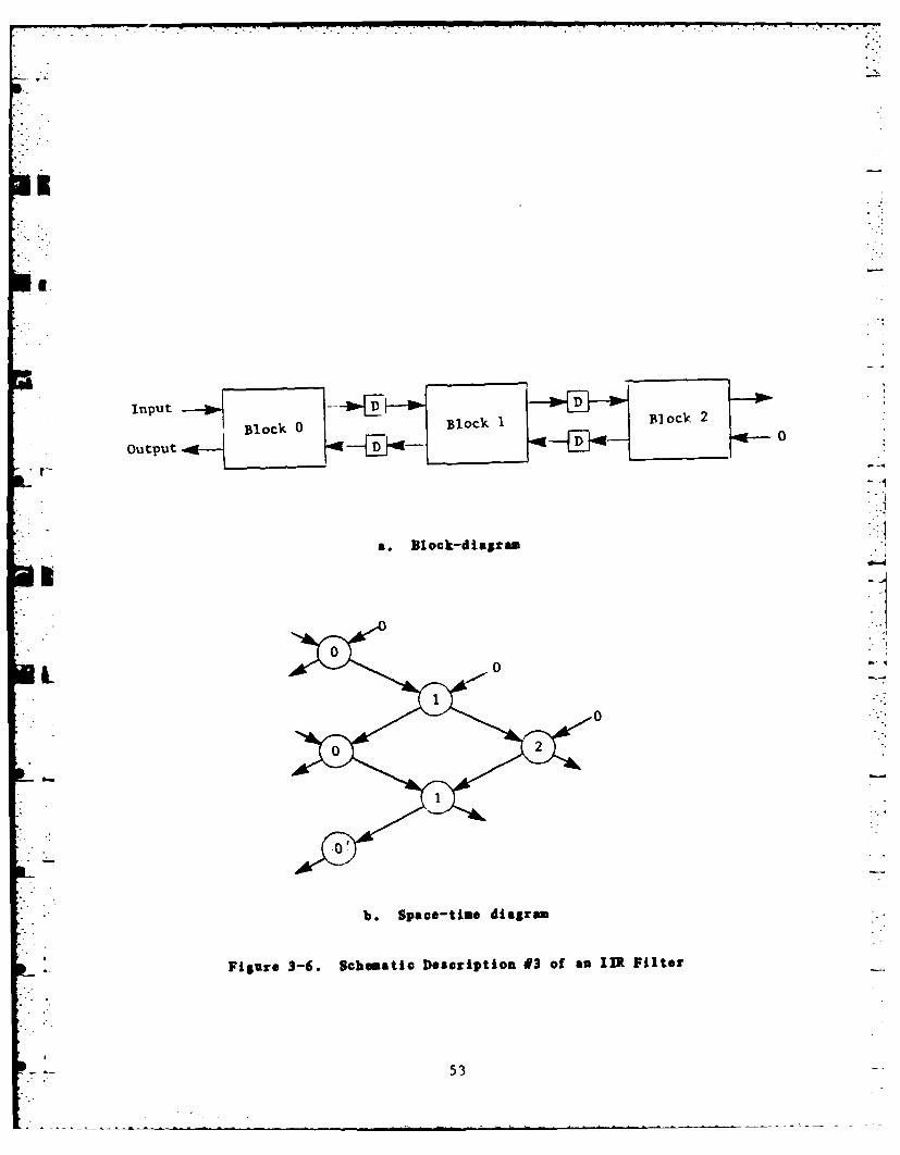
path (Figure 3-S) or split between the two signal paths (Figure 3-6). The
latter version is the only one that can be implemented in hardware because
- L it contains only downward-pointing arrows; the other two versions
require instantaneous evaluation of each variable associated with a
horizontal arrow. The third description makes it also clear that the time
interval between successive application of inputs is equal to two delay
units. It is also possible to associate unequal computing times with the
forward and backward propagation through each block. After all, the forward
path only feeds information through the block while the backward path
involves a multiply-and-add operation. The resulting space-time diagram
(Figure 3-7) has delays TfV Tb associated with the forward and backward
paths, and the input interval is clearly Tf * Tb. Notice that the block
diagram description involves two different delay blocks: This is known as a
sultirate implementation (8]. The throughput rates are, nevertheless, equal
to (Tf * Tb) -1 for both the input and the output.
The same technique can be applied to analyze the several proposed
systolic-array-like implementations for matrix multiplication: the
49

hexagonal array of H.T. Kung (5). the improved hexagonal array of Weiser and
Davis [4], the wavefront array processor of S.Y. Kung (7] and the direct
form realization of S. Rao [10]. Details are provided in Appendix E.
The analysis of the previous examples makes it clear that the common
MCN architecture shared by all the representations of a given processing
system induces certain invariants. For instance, the total number of
outputs of each processor remains invariant, even though in some
representations some of these outputs are connected to a local memory rather
than to a nearby processor (Figure 3-8). The same is true for the total
number of inputs of each processor. Notice that the blocks in Figure 3-8a
are still the same as in Figure 3-4a. including the orientation of paths
(one forward, one backward). On the other hand, the roles of the blocks are
quite different; in particular, outputs are obtained from the local memories
rather than from the left-most block alone, as in Figure 3-4a.
5
I-I

Block 0 Block I Block 2
Inu
a 2
a. Block-diagram
b. Space-tine diagram
Figure 3-4. Schematic Description #1 of an 11R Filter
51

Input N
Block Block 1 Block 2
OutputD
a. Dlock-41&Sram
522
Input Bok1B cBlock 00
Output -L-
a. Block-dia~ram
IL- 0
b. Space-time diagram
Figure 3-6. Schematic Description #3 of an 11R Filter
53

Input f HO T Ni
Block0 Blok I Bock
OutpU14- of
a. Blck dagra
0-0-
TI
Tf
Tb 0
011
b. Space-tim. diagram
Figure 3-7. Nultirate Implementation of an Ilk Filter (T f (Tb)
54

a. Block diagram
0 0
I-If
b. spc-tm S igr
Figure 3-8. Schematic Representation of TI Filter Involving Local Memory
'5- 55

3.5 SUMMARY
Techniques for analysis of pipelinability. schedules, and throughput in 4
systolic-array-like configurations have been developed based on the MCN
representation of parallel algorithms/architectures. Architecture
evaluation was also based on graph theoretic properties of the M10 model:
The dimensionality, degree of parallelism, and throughput of a given
architecture are all determined by analysis of its precedence graph.
The major difficulty in the analysis of computing networks lies in the
translation of low-level input-output relations to high-level ones, and vice
versa. We have shown that the problem reduces to the factorization of the
global (high-level) input-output map into a product of purely parallel maps,
corresponding to the concept of vavefront propagation in the network. More
specifically, the global input-output map is a sequential composition of the
maps corresponding to the layers of an execution.
-a _
56 -1_

SECTION 4
ITERATIVE AND COPLETELY REGULAR NETWOM
4.1 ITERATIVE MQCs AND HARDWARE ARCHITECTURES
An MCN is called iterative when it can be described as a sequential
composition of identical subnetworks, i.e.,
astwork - .
Each of the identical components ( will be called an iteration. One
reason for this name is that the MC can be executed by implementing a
single component Z in hardware and simulating a sequential composition of
such components by spreading the execution of the components in time. The
3 motivation for studying iterative MCNs is that most signal-processing
algorithms and, in particular, all systolic-array-like architectures can be
described by such networks. Observe that every block-diagram representation
corresponds to an iterative M10. The iterative structure induces certain
regularity constraints upon the 0N1 which lead to a simplified
representation.
The minimal schedules of iterative networks are, cleasly, periodic with
the same period for input and output schedules. Thus iterative MCNs are
temporally-regular. In addition, they are functionally-reaular in the sense
that each iteration involves the same function J. Consequently, their
properties can be determined by analyzing a single iteration. For instance,
the entire network is acyclic (hence executable) if a single iteration is
acyclic. In particular, the executability of z-transform representations of
iterative MCqs is tested by removing all separators and examining the
remaining directed graph for occurrence of cycles (see also [9]).
. Similarly, the (minimal) schedule of the network can be determined by
considering a single iteration.
57

rU
Iterative MCNs are commonly described by recursion equations (or
equivalently by z-transform diagrams), data-flow diagrams (marked graphs),
or by 'do-loops' in high-level programming languages. While precedence
graphs of iterative networks still indicate all possible executions,
recursion equations restrict the choice of execution to one or at most two
possibilities (Figure 4-1). And while precedence graphs avoid the pitfall
of non-executable iteration by explicitly describing each iteration as part
of an executable (acyclic) precedence graph, data-flow diagrams contain
cycles which may cause the entire M(N to be non-executable.
Since all iterations are identical, the schedules of every two
consecutive iterations differ by the same constant, which we shall call the
input interval. The input interval is the period of the input schedule or.
equivalently, of the input throughput, as well as of the output schedule
(recall that iterative MCIs are temporally regular). It determines an upper --
bound on the rate at which inputs are applied to the network (lower rates
are permitted, but require additional buffering).
The time-space diagram of an iterative MCN corresponds to its minimal
schedule and is, therefore, periodic. It is important to notice that the
period (= input interval) is, in general, shorter than the time required to
complete the execution of a single iteration (- the iteration delay). This
means that hardware realizations of the MCN can be pipelined: New inputs
can be applied before the processing of previous inputs has been completed.
The functional regularity of iterative MCNs implies that they can be
implemented in special purpose VLSI hardware by mapping the precedence graph
of a single iteration directly into silicon. Each processor is mapped into
a cell ('processing element') and precedence relations are mapped into
interconnections between cells. Neither translation nor hardware
compilation are required to accomplish this mapping since the hardware
architecture is an exact image of a single layer of the network
architecture. An execution is now interpreted as the propagation of a
sequence of wavefronts through the hardware rather than the propagation of a
single activity wavefront through the iterative MCN (Figure 4-2). The time
spacing of these wavefronts equals the period of the underlying MC4 minimal
schedule.
58 0

r
* 9.
599
a. Parallel lput Aiplioaton ..
/-
. b . 3 q u e t l l uI p u t A p p l i c a t i o n -.
, lFiure 4-1. Iquivaleat Pipelned Ezeoutiona of an NCd.
L 59

Since a single layer of the NCN is used to 'simulate' the entire
network each processor is activated many times and each arc of the hardware
architecture corresponds to a time-series of variables rather than to a
single variable. This raises a design problem of a new kind: It is
necessary to guarantee that variables do not disappear before they have been
used to evaluate their successors. There are three different solutions to
this problem:
(1) Iterative execution: A new iteration is initiated only after theexecution of the preceding iteration has been completed. Thismeans that the input interval is extended (by buffering ofintermediate results) to the length of the iteration delay, andthe time-overlap between iterations is completely eliminated.
(2) Scheduled execution: The (minimal) schedule of the network isdetermined in advance and execution is carried out according toschedule. Buffering is provided to guarantee the availability of - -.
inputs to processors on schedule (only non-critical variables needto be buffered).
(3) Self-timed execution: Processors are activated as soon as theirinputs become available. Acknowledgment signals ("hand-shaking')are used to guarantee the correct transfer of data between.- .processors.
While scheduled execution offers the shortest execution time and requires a
fairly simple control system, it is extremely sensitive to scheduling
perturbations. Such perturbations, which are caused by clock-skewing and 4
local variations in execution times, may result in loss of synchronization
between cells and a complete failure of the system. Iterative execution is
insensitive to scheduling perturbations and requires a very simple control
system, but wastes processing time since the hardware is idle most of the
time. Self-timed execution provides a nice tradeoff between these two
extremes: Its execution time is only slightly longer than the theoretical
minimum achieved by scheduled execution; and the control system it requires
has about the same complexity as the timing system for scheduled execution.
It is interesting to observe that the conditions for self-timed execution
(16], (17] coincide with the concept of admissible composition, which was
shown to be the necessary and sufficient condition for executability in
general. Thus, every NCI can be implemented as a self-timed system. -
60 1

-~~~~ ~~~ -- , -- - - -
b . Narwr rcietr Perspective r
Figure 4-2. Execution Interpreted as Activity Wavefront Propagation'
61 ...
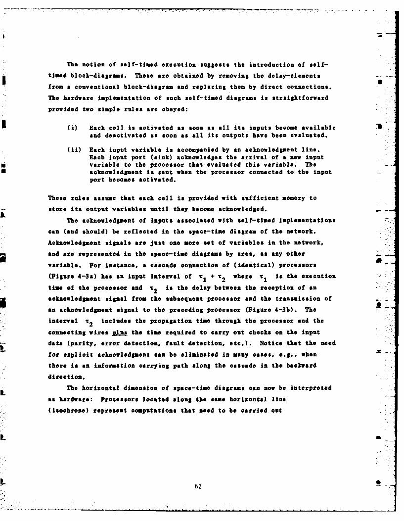
The notion of self-timed execution suggests the introduction of self-
timed block-diagrams. These are obtained by removing the delay-elements
from a conventional block-diagram and replacing them by direct connections.
The hardware implementation of such self-timed diagrams is straightforward
provided two simple rules are obeyed:
(i) Each cell is activated as soon as all its inputs become availableand deactivated as soon as all its outputs have been evaluated.
(ii) Each input variable is accompanied by an acknowledgment line.Each input port (sink) acknowledges the arrival of a new inputvariable to the processor that evaluated this variable. The --
acknowledgment is sent when the processor connected to the inputport becomes activated.
These rules assume that each cell is provided with sufficient memory to
store its output variables until they become acknowledged. -
The acknowledgment of inputs associated with self-timed implementations
can (and should) be reflected in the space-time diagram of the network.
Acknowledgment signals are just one more set of variables in the network,
and are represented in the space-time diagrams by arcs, as any other -
variable. For instance, a cascade connection of (identical) processors ja
(Figure 4-3a) has an input interval of v + T2 where v1 is the execution1'. 2 1
time of the processor and :2 is the delay between the reception of an
acknowledgment signal from the subsequent processor and the transmission of
an acknowledgment signal to the preceding processor (Figure 4-3b). The
interval v2 includes the propagation time through the processor and the
connecting wires yLus the time required to carry out checks on the input
data (parity, error detection, fault detection, etc.). Notice that the need
for explicit acknowledgment can be eliminated in many cases, e.g., when .
there is an information carrying path along the cascade in the backward
direction.
The horizontal dimension of space-time diagrams can now be interpreted
as hardware: Processors located along the same horizontal line
(isochrone) represent computations that need to be carried out
L &
62
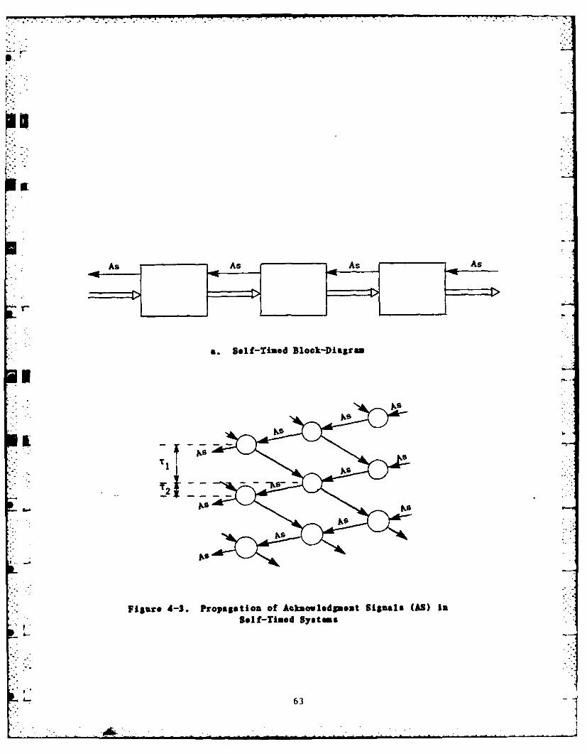
a. Self-Tined Block-Diagram
.N1
INIS
Figure 4-3. Propagation of Acknowledgment Signals (AS) isSelf-Time4 Systems
63
simultaneously and must, therefore, be implemented in parallel hardware. We
shall adopt the convention of interpreting the vertical dimension of space-
time diagrams as pure time: Processors located along the same vertical line
will represent computations that are carried out by the same processing
element but during different (non-overlapping) intervals of time. Thus, for
instance, the MCN of Figure 4-4 can be implemented in hardware with four 7.
processing elements (Figure 4-4b). Each vertical column of processors in
the space-time diagram of the M(C (Figure 4-4a) is mapped into a single
hardware cell; connections between columns are mapped into physical
connections between cells and connections within columns are implemented by
locally storing intermediate results inside the appropriate cells.
Self-timed or scheduled execution is, indeed, faster than iterative
execution only if the input interval is shorter than the execution time of a
single iteration. An implementation of such an execution will initiate a -
new iteration before the execution of the previous iteration has been
completed. Such implementations deserve to be called pipelined. Thus,
iterative executions are never pipelined, while self-timed (or scheduled)
executions are pipelined only for pipelinable MCNs.
Notice that the input interval is uniquely defined for every
temporally-regular 1N0, but the iteration delay (= execution time of a
single iteration) depends upon the partitioning of the 1N0 into iterations.
Since this partitioning need not be unique, an iterative MCN may have
several hardware realizations, each with a different iteration delay. Thus,
pipelining is primarily a property of a given hardware realization. An 1NI
is considered vinelinable if it has at least one pipelined realization.
Pipelinability is most frequently associated with completely regular NCNs
(= systolic-array-like networks). The connection between complete -
regularity and pipelinability is discussed in the following section.
6_64

a.SaeTm iga
b. Spf-Tie BoDiagram
Figure 4-4. Hardware Implementation of an Iterative MCN.
65
0 2 4
S.50
b. Intrleavd For
Figue 45. Rsouce harig b Intrlevin
'S 66

. . .. . . . .. 7
4.2 COMPLETELY REGULAR 04 s
A completely regular M10 is one that can be represented by a regular
multidimensional grid, and in which all input-output maps associated with
the vertices are identical. Thus, the vertices of a completely regular 1CNn
can be mapped into points of the multidimensional grid Z in the
n-dimensional Euclidean space Rn. where Z denotes the set of integers;
the arcs of a completely regular MCN become vectors (n-tuples of real
numbers) representing the directed straight lines connecting points of the
grid Zn . Clearly, not all points in Zn correspond to vertices of the
N4. Those that do determine the domain of the 1CN in Zn. The
requirement of complete regularity translates into the statement that the
vectors (arcs) emanating from any point (vertex) in do not depend upon
the choice of vertex. Consequently, the entire 1CN is characterized by: .
1i) the set of dependence vectors Id1i emanating from a single
vertex;
(ii) the domain r z2;
and
(iii) the input-output map f
f: (xI .... ) -- > (Yls ... Yp
associated with every vertex in the domain r.
*: A curious consequence of this definition is that the input-output map f
- has the same number of inputs and outputs, since the number of arcs
emanating from a point in r is always the same as the number of arcsconverging to a point.
Not every set of dependence vectors (di) determines a valid 1CN. For
instance, the directed graph representing an 10N has to be acyclic. In
terms of dependence vectors this means that it is impossible to find
positive integers (ki) such that Tkid 0. Another requirement is
67

that the ancestry of every vertex v B r (i.e., the set of all points from
which v can be reached) has to be finite. This constraint is trivial if
r is a finite set; however, if r is infinite (as is often the case with a
signal processing algorithms) this constraint implies that r has to be
bounded in the directions (-d ).
In the sequel we shall focus upon completely regular MCNs in Z$ ,
because such MCNs correspond to space-time representation of planar
systolic-array-like architectures (see [23] - [31]). We shall impose the
constraint of causality resulting from the association of 'time' with one of
3the coordinate axes in Z and examine the flow of data through the
architecture in terms of the dependence vectors characterizing the Nl.
4.2.1 Supace-Time Reupresentations in Z
CNs in Z are characterized by 3-dimensional dependence vectors
(di), which we shall represent by row vectors of length 3. The collection
of all dependence vectors -
D := [d ] (4.1)
forms a pxn matrix, which we shall call the dependence matrix. The
boundary of the domain r can always be described as a polyhedron. It will
be sufficient for our purposes to consider only convex polyhedra, and in
fact, only those that can be characterized in terms of the dependence
vectors (see Section 5.4 for a further discussion of this choice).
The interpretation of MCNs in Z3 as space-time representations of --
hardware architectures imposes the additional constraint of causality:
every dependence vector must have a positive time coordinate, since
computation and propagation of data cannot be accomplished in zero time.
Moreover, since data cannot propagate faster than the speed of
electromagnetic waves in metallic conductors, the directions of dependence
vectors must lie within a certain cone, the time-like cone in the space-time
continuum. By appropriate scaling of space and time coordinates we can
reduce this condition to the requirement
68

d [0 0 11 2 (4.2)
I which means that the third coordinate of di must be (an integer) larger or
equal to 1.
The association of time with the third coordinate of dependence vectors
allows us to express the finite ancestry condition in simple form. The
exclusion of ancestors that are infinitely remote from a given vertex in the
domain r is equivalent to the requirement that r be a subspace of the
positive half space of Z , i.e., the half space corresponding to non-
negative time coordinates. Moreover, since hardware must always be finite,
the spatial extent of r must be bounded. Thus, the only direction in
which r may remain unbounded is that of positive time, corresponding to a
* computation that continues indefinitely in time (e.g., a filtering of an
infinite time-series), but produces results (outputs) at regular intervals.
Vertices in r that share the same spatial coordinates are considered
as representing the same hardware processor at different instances in time.
* Regularity implies that such isospatial vertices are spread in time at
regular intervals. This interval, which is the same for all processors,
*m will be called the periodicity index of the architecture. The periodicity
- .index corresponding to a given dependence matrix D is the smallest
solution n of the equation
"LAD x (0 0 11 (4.3)
where A is any row vector with integer (possibly negative) entries. To
prove this result we notice that AD is an integer combination of
dependence vectors; moreover, if v(xl,Yl,t1 ) and v(x2,y2 ,t2 ) are two
distinct vertices in r, then the vector connecting these vertices can
always be expressed in the form AD for an appropriate (possibly nonunique)
* - row vector A. If the two vertices share the same spatial coordinates, then
their interconnecting vector is colinear with [0 0 1], and so (4.3) is
* - satisfied for some Aw. Finally, the smallest temporal displacement is
obtained when % is minimized in (4.3). The periodicity index it can,
actually, be evaluated without an exhaustive search through all possible
Integer vectors of A that satisfy (4.3), as is demonstrated in Section
4.2.2.
69

. . . . -.
The most important attribute of the space-time representation of a
completely regular M(0 is the invariance of the NCN under coordinate
transformations in space-time. This is so because coordinate
transformations do not affect the interconnection pattern of the space-time
representation, and consequently leave the corresponding directed graph
unaltered. In the case of regular space-time representations it is
sufficient to consider the effect of linear coordinate transformations; this
is done in detail in Sections 5 and 6.
4.2.2 Snatial Prolection of 1(4s in Z3
The first two coordinates in a three-dimensional space-time can be
interpreted as physical space. When a space-time representation is -
projected into the plane formed by the first two coordinates, vertices
represent computing agents (i.e., processors) and arcs represent physical
interconnections (i.e., wires). The projection amounts to the truncation of
each dependence vector to its first two coordinates, viz., .
D : 0 1 (4.4)0 0]
The truncated dependence matrix D ('a' stands for 'spatial') is usually -
sufficient to characterize the architecture, since we commonly assume that
each dependence vector represents a computation that requires a unit of
time, and consequently
D =D (4.5)
This assumption is violated only when D has a periodicity index x(D) ) 1
and, in addition, D contains a dependence vector of the form [0 0 v].
This dependence vector is truncated to [0 01, so v cannot be recovered
unless v = w or v - 1. These, in fact, are the only two possible values
for v as explained in Section 6.4.
70 I

The truncated dependence matrix can be pictorially represented by a
conventional block-diagram such as Figure 4-5. Each truncated dependence
vector is represented by an arc with the appropriate spatial displacement,
while truncated dependence vectors of the form [0 0], which correspond
to local memory, are represented by self-arcs.
a. Block-Diagram Representation
D = 0 1 D -1 00 0 0 f
' " b. Dependence and Truncated Dependence Matrices
Figure 4-5. Example of a Regular Hardware Architecture
71

La
The truncated equivalent of (4.3) becomes
s - 0 (4.6) 4
so that every feasible choice of q corresponds to an undirected loop in
the 2-dimensional block-diagram representation. Thus, every feasible q is
obtained by considering all possible loops in the block-diagram
representation. If there are no self-loops on vertices, then D contains
no zero row and (4.5) holds. Consequently, by (4.3),
tD[O 0 11 -e l 1 . . . l t
so n is obtained by adding up the entries of A. This is, in fact, done
by counting each arc along the loop as I if it coincides with the
orientation of the loop and as -1 if it points in the reverse direction.
Since the smallest value of fr is required, only the shortest loops need to
be considered. We shall show in Section 5.3 that a never exceeds 3 and is
seldom larger than 1. -
4.3 MODULAR DECOMPOSITION OF MCN MODELS
The conversion of a given algorithm into an 1CN model is based upon the
assumption that the fundamental building blocks--the processors--are
implementable in hardware. This is indeed so if each processor represents a
few scalar operations, which can be handled by any contemporary computing
agent. However, signal processing algorithms are rarely specified in this - .
convenient form; most often they are represented by block-diagrams whose
blocks involve multivariable manipulations, and in particular, matrix
algebra. The construction of a computer program or a hardware
implementation for such 101. requires to decompose each multichannel
processor into a subnetwork of scalar processors. One way to achieve this
decomposition is by storing standard subnetworks for commonly used
operations such as matrix addition, multiplication and inversion in a-A
library and invoke this information whenever the need arises. However, the --
experience with signal processing schemes indicates that better results are
72

' ' -?- ~ f
obtained by matching the method of decomposition to the structure of the
problem. By a Judicious application of the principle of modular
decomposition [32] we obtain completely regular MOCs which are perfectly
suited for implementation in VLSI, and have a much higher throughput than
those obtained by mapping matrix operations directly into parallel hardware.
There is, at present, no simple test to establish the applicability ofiLthe principle of modular decomposition to a given multichannel operation.
When the operation is linear in all its operands the necessary and
sufficient conditions for modular decomposability can be stated in simple
terms as described below.
4.3.1 Modular Decomposition of Linear Multivariable Filters
Let 1(z) be the transfer function of a multivariable filter with an
* equal number of inputs and outputs. Suppose that the inputs have been
aggregated into three multichannel inputs x, u1 , u2 and the outputs have
been respectively aggregated into w, y1, y2 (Figure 4-6). Thus,.1 1 (z)Z(z)
C2:() B (z) u (z) (4.7)
Iwz J u 2(z)
. Suppose that there exist transfer functions B (z), H(z) such that
) [(4.8)
where p is the number of channels in u1 and q is the number of channels
in U2 . Then the filter can be, clearly, decomposed in the form described
by Figure 4-6. Conversely, if such a decomposition exists, then (4.8) will
hold. Thus, the existence of the factorization (4.8) is a necessary and
sufficient condition for the decomposability of a multivariable filter as
described by Figure 4-6.
A_ 73
". ,-. -.

U1 y1
U2 2
a. Before Decomposition
U 2 2()Y
V v
b. After Decomposition
Figure 4-6. Modular Decomposition of a Linear Multivariabi. Filter
74

*,- - -
To make the decomposability condition more explicit we sball describe
the transfer functions nl(z) in terms of blocks, viz.,
1(z-N ) - , = 1,2 (4.9)WCi() D(z)]
.oc
The corresponding decomposition of 1(z) yields, via (4.8). (4.9) the
identity
Hii~) 1(z) 113(z)] A1(z) B IzW 01
1(z, .. 21() ,22 (z) ,23(z) A2 (z)C1 (z) A(z)D,(.) 22 2 (z)
L H (z) W (z) H(z) C (z)C ( -) CW(z)W (z) ()31 32 3 3 [2 1 2 2 2
14.10)
This means that some elements of R (z) can be uniquely determined from
those of the given H(z), for instance
A1 (z) = l (z), D2 (z) - 3 3 (z). etc.
i- .Since the blocks B z), C (z) are square (while Ait Di need not be
* square), we also obtain, assuming nonsingularity of square transfer
L functions
A1z) 2z)C 1 z) (4.11a)2 B21 1
which implies
L (z)C 1 1Z)D(z) - 2 (z) (4.11b)
Similarly
c(z)H 1z z) (4.12a) )
2 3 1 ( ) 1
which implies
• f75

H 31zWC I I(z))2(Z (4.12b)
"31 1) D1 32(z)
which means that for all z
rank Sn
B 31(Z) 2( Z
where n is the number of channels in the signals x, v, w. In fact. if we
insist that square transfer functions are, generically, invertible, then
1 (z) is an nxn nonsingular matrix, so that--31
H (Z) H (Z)21 22
rank -n (4.13b)
f31 () 932(Z
Conversely, If (4.13b) holds, then
C711 ( z)Dl(z) - H31(z)132(z) (4.14) -
Choosing C1(z) arbitrarily we obtain A2(z). C2 (z), D I(z) via (4.11a).
(4.12a) and (4.14). respectively.
In summary, a necessary and sufficient condition for a decomposition of
the form (4.10) to exist Is that the rank condition (4.13b) holds and in
addi tion
B (Z) 0 (4.15)13
76Ito

-7S
Given a transfer function H(z) that satisfies the decomposability
conditions we can always compute B I(z), 8 . In fact. we may choose
C (z) arbitrarily, and the simplest choice is --C (z) 1. This yields the
* decomposition
-P 0 0 [ 11 (Z) N12 (Z) 0]H~) I 21(z) m7,lH3(z)%32(z) o (4.16)
[o H1( z) H()J [0 0 J
a-
177

- -. - -- - -. - -- - N14
786

SELTION 5
CLASSIFICATION OF ARCHITECrURES
Completely regular M(4s were characterized in the previous section in
terms of their dependence vectors. It was also indicated that XCNs with
different dependence vectort may nevertheless be equivalent, namely they
will have equivalent space-time representations. The equivalence of
completely regular M(4s is easy to verify, since it amounts to the existence
of a nonsingular linear transformation relating the dependence matrices of
the 104s in consideration.
The study of equivalence can be carried out at several different levels
of abstraction. At the lowest (most detailed) level each completely regular
1CN is represented by a dependence matrix
D ]5.1)
where di are row vectors of length 3 whose first two coordinates represent
the planar space of integrated circuits and the third coordinate represents
time. Thus, for instance, the M10 of Figure 5-1 is characterized by the
dependence matrix
Dm[ 1 .1 0
Notice that the time coordinate of all three dependence vectors equals to 1.
reflecting the assumption that each dependence vector represents a
computation that requires a unit of time. This assumption can, of course,
be modified to incorporate computations with unequal processing times.
Notice also that the direction of dependence vectors coincides with that of
the arrows in Figure 5-1, pointing toward the successors of a given
processor, rather than toward the predecessors of the same processor, as in [25].
79

yI'
Figure 5-1. Example of a Completely Regular 10N
At the intermediate level of abstraction only the spatial coordinates
of each dependence vector are considered. This results in the elimination
of the third column of the dependence matrix D, resulting in the truncated
dependence matrix D
D 0 1
for the example of Figure 5-i. We shall show in the following section that
the truncated dependence matrix D provides, in fact, a complete, albeit5
implicit, characterization of the M0. This characterization can be
transformed in a unique manner into the explicit characterization D.
At the highest level of abstraction only the topology of the hardware
is considered. This means that the directed graph representing the flow of
data is replaced by the corresponding non-directed graph. Thus, for
instance, the NCR of Figure 5-1 and that of Figure 5-2 are topologically
equivalent, even though the latter has a different depende-ce matrix, viz.
D 0_1
801

Figure 5-2. A Completely Regular IN Which is Topologically Equivalent
to that of Figure 5-I
This section is devoted to the study of topological equivalence
followed by the study of architectural. (D ) equivalence. The more
complicated topic of space-time equivalence is presented in the following
section, where it is also shown that distinct hardware configurations may,
nevertheless, have equivalent space-time representations.
* 5.1 TOPOLOGICAL BQUIVALENCE
The topic of topological equivalence has been studied by Niranker and
Winkler [25], who have shown that there are only three distinct topologies
(Figure 5-3):
(1) The linear topology, with a single dependence vector,
D =[1 01
(2) The rectangular topology, with two dependence vectors,
Ji o
D 1I
81

a. The Linear Topology
b. The Rectangular Topology
6. The Nexagonal Topology
Figure 5-3. The Three Fundamental Topologies
82

(3) The hexagonal topology, with three dependence vectors,
1 0]
Every systolic-array-like architecture can be related by a linear
transformation to one of these fundamental topologies. Also, it is
impossible to have more than three non-colinear dependence vectors in a
planar architecture.
The same conclusion can be reached by a graph-theoretic argument. The
graph describing the hardware configuration of a completely regular M10 is
clearly a mosaic, i.e., a planar graph in which all faces are bounded the
same number of edges and all vertices (except those on the external boundary
of the graph) have the same number of incident edges. As is well known,
there are only three possible mosaics [21]: triangular, rectangular and
" hexagonal. The triangular mosaic has vertices of degree 6 and coincides
with the hexagonal topology. The rectangular mosaic has vertices of degree
4 and coincides with the rectangular topology. The hexagonal mosaic (Figure
5-4) does not correspond to a completely regular MC0, since it requires two
sets of dependence vectors rather than one. However, it can be rearranged
by combining pairs of adjacent processors into a single processor (Figure 5-
4b). so that the resulting configuration has a rectangular topology. Thus,
there are only two mosaics corresponding to completely regular MCNs, which
-] combined with the linear configuration makes a total of 3 fundamental
- topologies.
L8-
L 3 L_

a. The Mosaic
b. Rearrangement as a Rectangular Topology
Figure 5-4. The Hexagonal Mosaic
84
27

5.2 ARCHITECTURAL BQUIVALENCE
.. Each of the interconnecting wires in the three fundamental topologies
can be associated with two direction vectors, one pointing along the wire in
one way, the other in the reverse. This makes a total of three
possibilities for each interconnecting wire: (i) + d, (ii) -d, and
* (iii) ± d. This means that the linear topology results in 31 = 3architectures, the rectangular topology in 32 = 9 architectures and the
hexagonal topology in 33 - 27 architectures. Since many of these
architectures are equivalent, a classification of the distinct architectures
is provided in Table 3-1. The nomenclature consists of a capital letter
(L, R or H) indicating the topology (linear, rectangular or hexagonal), a
digit indicating the number of dependence vectors and a lower case letter,
* whenever required, to distinguish between architectures which have the same
topology and the same number of dependence vectors but are not equivalent, L
e.g., H3a and 53b. The table lists all equivalent configurations in a
single row.
5.3 PERIODICITY ANALYSIS AND THROUGPUT
The occurrence of cycles (i.e., closed loops of directed arcs) in the
U directed graph representing a hardware architecture provides important
information about the throughput rate of the architecture. In this
. subsection we analyze this information and identify the configurations with
low throughput.
The periodicity index x of architectures has been defined in Section
4.2. It can be computed either by examining undirected loops in the graph
* representing the architecture or by solving the equation
Ds - 0 (5.2)
for every possible row vector A with integer elements, and summing the
elements of q. The periodicity index if equals the smallest of these" ,
85
1 - o . - - • - - -. _.

4
TABLE 5-1. CLASSIFICATION OF RARDWARE ARCHITECTURES
4
Pair I Pair 2 Pair 3
Li
L2
-R2I
R3
+ __r
R4.
113b
H4b
116
86
4h..

-n 77 t
r.
sums. If no solution ij exists, it is defined to be 1. Following this
technique we conclude that L, R2 have no solution and have a unit
periodicity index, while other architectures have solutions, as follows:
(i) L2 has v -(1 13; hence x 2.
J (ii) R3 has [1 1 0]; hence at 2.
(iii) R4 has q= [1 1 0 01, [0 0 1 11; hence vt 2.
(iv) W3a has ij [1 1 -1]; hence vt 1.
(v) B3b has wj [1 1 1]; hence a = 3.
(vi) H4a has l = [1 1 -1 01, [0 0 1 1], [1 1 0 11; hence xt 1.
(vii) H4b has ' - [1 -1 0 1], [0 0 1 1]; hence nt I.
(viii) HS has ( 1 (I 0 1 0 -13, [1 1 0 0 03, [0 0 1 1 01; hence
(ix) B6 has q = [1 0 1 0 -1 0], [1 1 0 0 0 0], [0 0 1 1 0 0].
[0 0 0 0 1 11; hence w -1.
In the sequel we shall measure the throughputs of architectures
relative to the throughput of the linear architecture LI (a classical
L. pipeline). Since the time interval between two successive applications of
input equals the periodicity index, the relative throughput of a givenarchitecture is given by the formula
relative throughput (5.3)periodicity index
Thus, the relative throughput of L2, R3, R4 is 1/2 and that of 93b is
1/3.
87

. 5.4 BOUNDARY ANALYSIS
No assumption has been made up to this point about the shape of the .4
boundary of a given hardware architecture. However, since the shape of the
boundary is channed by linear transformation it has to be taken into
consideration in the process of classifying architectures. As an example
consider the 6 equivalent configurations denoted by 3a (Table 5-1). The : .
truncated dependence matrices of the first and third of these configurations
are related by a linear transformation, viz.
Nov assume that the first configuration has a rectangular boundary, which
can be characterized by boundary matrix -:
8 0
D[1
consisting of all dependence vectors colinear with the boundary. The linear
transformation maps this boundary into
B, Bnas is ..]=~ 2~
which characterizes a parallelogram rather than a rectangle. Thus, the
first H3a configuration with a rectangular boundary is equivalent to the
third 93a configuration with a parallelogram boundary. It is not
equivalent, however, to the third M3a configuration with a rectangular
boundary. Clearly, we need to reclassify the entries of Table 5-i according
to both the dependence matrix and the boundary.
We shall be concerned only with boundaries that satisfy the two
following conditions:
(i) The boundary curve is a closed convex polygon
88r',imi

(ii) Each segment of the boundary curve is colinear with some
dependence vector.
Thus, the only possible directions for the segments of the boundary curve
* .- are [1 0]. [0 11 and [1 1]. Consequently, there are four possible
*boundary curves (Figure 5-5): rectangle, parallelogram, lower triangle,
* upper triangle. Of these, only the rectangle-shape boundary can be applied
to the linear (1) and rectangular (R) architectures. On the other hand, all
four possible boundaries can be combined with hexagonal (N) architectures.
However, since linear transformations map rectangles into parallelograms and
lower triangles into upper ones, we need only consider the combination of
each hexagonal entry of Table 5-1 with either a rectangular or a triangular
*- boundary.
L89

a. Rectangle
.
b. Parallelouram
a. Lower Triangl d. Upper Tniagle
Figure 5-5. Fundamental Boundary Curves
90I

TABLE 5-2. CLASSIFICATION OF HARDWARE ARCNITECTURESWITH RECTANGULAR BOUNDARIES
L21 R 2 R3 R4
1 0 1 0 1 0 1 0 1 0
-1 0 0 1 -1 0 -1 0
0 1 0 1
0 -1
!3aa 3ap 13b 4aa 4ap
1 0 -1 0 1 0 1 0 1 0
0 1 0 1 0 1 0 1 0 1/ L1 1 1 1 -1 -1 1 1 -1 0 -
-1 -1 -1 -1
B4ba 14bo B5Q RSA 16
1 0 1 0 1 0 1 0 1 0
0 -1 0 1 -1 0 -1 0 -1 0
1 1 0 -1 0 1 0 1 0 1
•""-1 -1 1 1 0 -1 1 1 1 1S1 0 -1 - 1 1 1
91. .-.- 9

J
With rectangular boundaries we need to consider matrices of the form
[Ba I(5.4)
Clearly .
[D1 -**~=[DS]
J
which shows that the reversal of all dependence vectors does not produce a .
new configuration. The 6 entries in each one of the rows H3a, 54a, H4b, I5
of Table 5-1 can, therefore, be considered as 3 pairs of conjugate
configurations. Of these, the second and third pair are still equivalent . -
when combined with rectangular boundaries, but the first pair is different.
Thus, the entries of Table 5-1, when combined with rectangular boundaries,
can be reclassified as in Table 5-2. This time each architecture is
specified by its D matrix rather than by a pictorial description as in
Table 5-1.
Similarly, we can combine each hexagonal entry of Table 5-1 with a - -
lower triangular boundary. This will again produce two distinct
architectures for each one of the rows I3a, H4a, H4b, IS. However, there
is no need to do it explicitly, since the resulting configurations can
always be obtained by 'cutting' the appropriate hexagonal topology combined
with a rectangular boundary along the main diagonal. Thus, it will be
sufficient to focus in the sequel upon rectangular boundaries alone.
5.5 SUNNARY
Systolic-array-like architectures have been classified by topology,
interconnection pattern and shape of boundary. We have shown that there are
only 15 distinct (non-equivalent) architectures (see Table 5-2). We have
also shown that it is sufficient to consider only rectangular boundaries
which are of practical importance in the process of VLSI layout. -
92 _

A genealogical chart (Figure 5-6) shows which architectures are
contained in any given architecture. In particular, it shows that H6 is
the 'universal architecture' for systolic arrays, containing every possible
architecture with a smaller number of dependence vectors.
Ll
I. -_
Io
115B:
Figure 5-6. Genealogical Chart for Architectures
. 93

AD-Ri46 030 ANALYSIS AND DESIGN METHODOLOGY FOR VLSI COMPUTING 2/2NETWORKS(U) INTEGRATED SYSTEMS INC PALO ALTO CAH LEY-RRI RUG 84 ISI-46 N88i4-83-C-0377
UNCLSSIFIED F/G 9/2 NL
mmons-mmhhihhlmEEEEmmiEmhmhEEmmmmmaimaiiEND

1.0.
VA- -.*,
-J,
liii L30 1 1-2
11111-2 LI1 11.6
p.'
MICROCOPY RESOL.UTION TEST CHARTNATIONAL BURiMJ OF STANDAR 1963-A
'o

SECTION 6
CLASSIFICATION OF SPACE-TIE EPSENTATIONS
The space-time representation of a completely regular CNG was
characterized in the previous section by the dependence matrix D. The
hardware configuration was obtained by focusing upon the spatial coordinates
of the dependence vectors, which resulted in the truncated dependence matrix
D . It was observed that the temporal coordinate of all the architectures5
described in Section 5 was always equal to 1. viz.,
D [Ds (6.1)
i so that the dependence matrix D can be easily reconstructed for any given
D via (6.1). The properties of the corresponding space-time diagram canthen be deduced by analysis of the dependence matrix D.
6.1 THE FUNDAMENTAL SPACE-TIME CONFIGURATIONS
Each of the fundamental 11 architectures of Table 5-2 determines a
fundamental space-time configuration. Ve shall focus our attention upon the
dependence matrix alone, without considering. for the present, the shape of
the boundary surface. Thus, equivalence between the fundamental space-time
configurations is established by relating the corresponding dependence
matrices by linear transformations. A simple analysis (see Appendix F)
shows that every dependence matrix with 2 vectors can be transformed into
the equivalent (canonical) form
D(2) [1 :10
PREVSPAGE
95

. .. . ,
and every dependence matrix with 3 vectors can be transformed into the
equivalent form
D1 0 1 010 0 1.
Consequently, L2 R 2 and R3 - H3a - 13b where the tilde (-) denotes
equivalence. For dependence matrices with more than 3 vectors it is
convenient to establish first a (nonunique) canonical equivalent, i.e., an
equivalent dependence matrix whose first three rows are the identity matrix,
viz.,
D =:D= 0 1
*Some canonical-form equivalents are listed in Table 6-1. The full list of
canonical equivalents will be discussed in later sections in conjunction
with the specification of boundary surfaces in the three-dimensional space- . _
time continuum.
6.2 ARCHITECTURES WITH LOCAL MEMORY g.iL--
The preceding analysis was based upon the assumption that processors
transmit the results of computations to their immediate neighbors and never
store them for further use. However, many applications do involve such P
storage; this is true, in particular, for adaptive system/parameter
identification algorithms that store the identified parameters in fixed
location within the array and use the signals that flow through each
processor to time-update the locally stored parameters. In this section we - - -
consider the architectures obtained by providing each processor with a local
memory.
O
96.

TABLE 6-1. CANONICAL FORM BQUIVALENTS FOR FUNDAMENTAL ARCHITECTURES
*Li L2,R2 R3, R3a13 b R4
1 0 0 1 0 0 1 0 0 1 0 0
0 1 0 0 1 0 0 1 0
0 0 1 0 0 11 -1 1 _
34a 84b N5 36
I.
1 0 0 1 0 0 1 0 0 1 0 0
0 1 0 0 1 0 0 1 0 0 1 0
0 0 1 0 0 1 00 1 0 0 1
*3/2 -1 1/2 -1/2 1 1/2 -1/2 1 1/2 -1/2 1 1/2
3/2 -1 1/2
97

Topologically, local memory means the addition of a self-loop to each
processor (Figure 6-1). The direction of each interconnecting link can
still be chosen in 3 distinct ways, as explained in Section 5.2. resulting
in 11 new architectures (Table 6-2). Two important observations have to be
made regarding this table:
(i) The number of dependence vectors is larger by one than the number
of interconnections. Thus, for instance, RN3 has 4 direction
vectors, not 3.
(ii) The length of the last dependence vector, corresponding to the
local memory, equals the temporal displacement between two
consecutive occurrences of the same processor in the space-time
configuration. Thus, in general, this displacement is 1, except
for L2, R3, R4 whose temporal displacement is 2 (corresponding to
a periodicity index of 2), and except for B3b whose temporal
displacement is 3 (corresponding to a periodicity index of 3).
Local memory can also be used to interleave computations and achieve .
increased throughput with architectures whose relative throughput without
memory is less than 1. This possibility will be discussed in Section 6.4.
Analysis of equivalence between space-time configurations with local
memory reveals that:
(i) Iii, which has 2 linearly independent dependence vectors, is
equivalent to L2, 12.
(ii) R2, which has 3 linearly independent dependence vectors is
equivalent to R3, 3a, H3b.
(iiI) hW3a, which has 4 dependence vectors, is equivalent to R4.
In all three cases we can trade interconnecting links for memory, thereby
98
1

a. The Linear Topology with Memory (LI)
b. The Rectagular Topology with Memory (IN)
Go The Nexagonal Topology with Memory (M
Figure 6-1. The Three Fundamental Topologies with Local Memory
I 99
..1-._:'.- -- ,-.. . 7.";" -.- :-. ° " . '" ":v . , - - .7 .: - ..- , .: _.Y"-. - - .: - - .;7 ; '- . _ . , . . .'-..,-,

...--. ... . • _ . i . .
TABLE 6-2. THE FUNDAMENTAL BARDWARE ARQIITECTURES WITH LOCAL MEMORY
Imi LJ12 330 3313 33
1 0 1 1 0 1 1 0 1 1 0 1 1 0 1
0 0 1 -1 0 1 0 1 1 -1 0 1 -1 0 1
0 0 2 0 0 1 0 1 1 0 1 1
0 0 2 0 -1 -1
0 0 2
13 DX3b M14a =4b IS 336
1 0 1 1 0 1 1 0 1 1 0 1 1 0 1 101 , _
0 1 1 0 1 1 0 1 1 0 -1 1 -1 0 1 -1 0 1
111 -- 11 111 11 1 0 1 1 0 1 1
0 0 1 0 0 3 -1-11 -1 -1 1 0 -1 1 0 -1 1
0 0 1 0 01 1 11 1 1"
0 0 1 -1 -1 10 0 1..-.!
100

reducing the number of physical wires required to construct a realization of
the architecture and simplifying the layout problem for VLSI implementation.
Thus, for instance, the R2 architecture which requires a planar network of S
processors with 4 interconnecting ports at each'processor can be replaced by
LKI which requires a linear network of processors with 2 interconnecting
ports at each processor and a local memory. Even more remarkably, the same
replacement also trades low throughput configurations for high throughput S
one s.
6.3 BOUNDARY ANALYSIS S
The relation between boundary shapes and equivalence between (planar)
architectures has been examined in Section 5.4 The combination of topology
and boundary has produced 15 distinct architectures which were summarized in p
Table 5-2. Since each one of these architectures has a rectangular
boundary, the resulting space-time configuration always occupies a
rectangular prism (with the exception of low-dimensional architectures such
I as Li, L2, R2 whose space-time configurations occupy 1 or 2-dimensional -
subspaces).
Since linear transformations change the shape of the boundary, the
equivalence between space-time configuration, discussed in Sections 6.1 -
n 6.2. has to be reexamined to include the effects of boundary
transformations. It will be sufficient to carry out this analysis only for
collections of space-time configurations which have been declared as
equivalent in the preceding sections.
6.3.1 The Confiturations LM. L2. R2
The configurations Il, R2 can be considered equivalent only when we
assume that a single set of inputs is applied to R2 (rather than a time- .
series). In this case R2 is characterized by
0 1 1
0 1 1 " -
L 101 -i.?

* while Liii is characterized by
[D] 0 [I 1and the two are equivalent, being related by a linear transformation, viz., -
On the other hand, Liii and 32 are not equivalent to L2 for which -
The P-part of this characterization can be related to the D-part of LMi.
viz.#
where the asterisks denote entries which can be chosen arbitrarily (subject
to the nonsingularity constraint of the linear transformation). However,
when the dependence matrix is combined with the boundary matrix we obtain
1 j1 001 [1 01
0 1 [0: 1jl. _I 0 1 -
which does not match the 3-part of 12. When the inverse of this
transformation is applied to the dependence and boundary matrices of L2.
viz.#
1- i-1- 1 0 1 0-07 -1-10 0) 1m / 0 1j
102
4o

apace
IA time
L
'010

the resulting configuration (Figure 6-2) is equivalent to an LMI
configuration of infinite order; the finite active part of the architecture
is shifted one cell to the right every time a new input is applied. Thus,
in summary. LKI and R2 are equivalent to each other but not to L2.
6.3.2 The Configurations RM2. 3. Ms. H3b 71
The truncated boundary matrix of these configurations was chosen in
Section 5.4 as
namely, the rectangular boundary. The corresponding boundary surface in the
space-time continuum is, therefore, characterized by the boundary matrix
B= 1 (6.1)01
When this boundary matrix is combined with the dependence matrices of DM2,
R3, H3a•, aO, R3b, equivalence is destroyed. For instance, trying to
relate Mau to RM2 we obtain
[1 0 1 1 0- 1
] I 1 1 0
0 5 L10
The resulting D-part coincides with the dependence matrix of RM2, but the
boundary surface is different. The configuration obtained above by
transforming H3aa is in fact an RM2 hardware of infinite order in which
a finite active segment shifts along the diagonal by one cell each time a
set of inputs is applied to the array. This is, in fact, precisely what
happens in systolic arrays for matrix multiplication. The configuration
Da* (of Weiser and Davis [4)) is suited for multiplying banded matrices.
When the same problem is implemented on an RM2 configuration (of S.Y. Kung
[71) most cells in the array are idle while a small active rectangle,
104

corresponding to the bandwidth of the given matrices, shifts along the main
diagonal of the array. In analogy, while multiplying two matrices with no
structure is carried out efficiently by an R33 array, solving the same -
problem on an 93a configuration involves many' idle cells and a small
active segment that shifts along the main diagonal.
6.3.3 The Configurations HM.a, R4
These configurations have the same boundary matrix, given by (6.1), as
RN2, R3. 13a and H3b. Since their dependence matrices are different, we
conclude that m/3aa. HM3ap, R4 are distinct configurations when the shape
of boundary surface is taken into account.
6.3.4 Summa"
When boundary considerations are taken into account each of the 15
architectures of Table 5-2 is distinct and cannot be related by equivalence
to any other architecture in this table. Incorporating local memory results
in doubling the total number of distinct configurations to 30.
6.4 INTrMLEAVING ARC(ITECTU3ES BY LOCAL NMORY
The introduction of local memory in Section 6.2 involved the assumption
that locally stored data remain in memory until required, which makes _
particular sense in data driven realization. Consequently, the duration of
storage for some architectures (L2, R3, R4, H3b) was longer than one time
unit. This fact can be used to construct new architectures with higher
throughput, by interleaving computations in time and connecting the
interleaved computations via the local memory.
The simplest example of such construction is the architecture L2.
Without interleaving the-throughput of L2, UM is 1/2 (Figure 6-3a).
With interleaving, which involves superimposing in time two L2 schemes and 0
interconnecting them via local memory, the resulting LiN2 configuration
105 0

space
time
21
a. Without Interleaving (L112)
space-
time
b. With Isterleaviss M02v)
Figure 6-3. Interleaving via Local Memory
106 _

-.
(Figure 6-3b) has throughput = 1. A similar approach produces the
architectures RIM3, RiM and 1iM3b, whose characterizations are given in
Table 6-3. The difference between these architectures and their
noninterleaved counterparts is the shortening of the local memory dependence
vector from either [0 0 21 or [0 0 31 to [0 0 1].
* S
TABLE 6-3. DEPENDENCE MATI[C.8 ]MR INTERLEAVED AR ITECTURES
LiJO Ri RM RiM3b
1 0 1 1 0 1 1 0 1 1 0 1
-1 0 1 -1 0 1 -1 0 1 0 1 1
0 0 1 0 1 1 0 1 1 -1 -1 1
0 0 1 0-1 1 0 0 10 0 1
6.5 SUMMARY
* Space-time configurations have been classified by topology,
interconnection pattern, shape of boundary, existence of local memory andinterleaving. The 15 fundamental architectures of Table 5-2 give rise to
another 15 configurations involving local memory. These, in turn, give rise
-. to 4 interleaved configurations, producing a total of 34 distinct space-time .
configurations.
L. 107

-_. . . _ . : . . . . = . . - - -.. . . . . . . .- " " : 2 . ... . . . .'- - - -.-... - ..- - .
Ignoring the shape of the boundary surface results in 20 distinct
configurations:
I
1) I 11) B4au, H4aP
2) IMI, L2, R2 12) B4b, H4bP
3) LN2 13) R94
4) Li2 14) RiM4
5) R32, 13, 3an, R3ap, 113b 15) HM44au, EM4ap
6) R3 16) 1144ba, BM4bP
7) RiM3 17) Ia., H5P
8) UM3aa, MNlap, R4 18) EI(Sa, HMP
9) EM3b 19) B6-
10) HiM3b 20) 1116
Ignoring, in addition, the details of local memory (and. consequently, of
interleaving) results in 8 distinct configurations only as in Table 6-1.
Choosing the optimal configuration for a given computational scheme
requires a specification of both the interconnection pattern and the
boundary shape. This can be accomplished only when specific details of the
corresponding computational scheme are taken into account (e.g., bandedness
of matrices to be multiplied). When only partial information is considered
the designer is often able to choose -the interconnection pattern but not the
boundary. Thus, multiplication of two matrices can be implemented in any of
the five equivalent hardware configurations 10 (7], R3 (10], M~aa [41,
Wag, 13b [5]. However, RN2 will be optimal if both matrices have no
particular structure; R3 will be optimal if only one of the matrices is
banded; and H3aa (or Mlap) will be optimal if both matrices are banded.
It is an historical curiosity that the first systolic array for matrix -
multiplication, R3b, is never optimal, because it has relative throughput
of 1/3 and is otherwise equivalent to 13a.
10
108

SECrO t 7
* S
A modeling and analysis methodoloty for parallel algorithms and
architectures has been presented, Modular computing networks (MCNs) were
introduced as a unifying conqept that *a* be used to describe both
algorithms a~d architectures. Th rtiresentation of an MCN exhibits all the
relevant information that characterizes a parallel processing aigorithm,
from precedence relations and order of execution, through scheduling and
r- pipelinability consideration, to map compositions and global
characterization. It clearly displays the hierarchical structure of a
parallel system and the multiplicity of choices for hardware implementation.
Our methodology applies both to arbitrary (irregular) networks and to
iterative ones. Regularity of networks translates directly into regularity
of the model we use to describe them and, consequently, into regularity of
the associated architectures. Problems of non-executability (deadlocks,
safeness, etc.) are insignificant in our methodology and can be easily
detected and resolved.
Infinite MCqs, which occur in most signal processing applications, have
been characterized. It has been shown that the key property for
executability of such networks is structural finiteness (in addition to
absence of cycles, of course). Infinite M(Ns are most frequently iterative,
.. in which case they are guaranteed to be structurally finite and can be
represented by a finite single-layer diagram.
Dimensionality, pipelinability and throughput have been introduced as
-fundamental structural attributes of MC models. Throughput computations
(see, e.g., [9]) have been established as a direct consequence of the notion
of schedule, which applies to every MCN model. The wavefront concept
[4,7,8] has been shown to be a natural outcome of associating schedules with
iterative networks. Systolic-array-like architectures were modeled and
analyzed via the concept of completely regular MCNs.
L 109

A classification of canonical realizations for completely regular
modular computing networks has been presented. Three levels of abstraction
were considered: topology, architecture and space-time representation. The 0
analysis revealed 3 canonical topologies, 15 canonical architectures and 34
canonical space-time configurations. It was shown that the unigue canonical
counterpart of any given topology, architecture or space-time configuration
is obtained via a simple (and unique) transformation of the corresponding -
dependence and boundary matrices. It was also shown that only rectangular
boundaries are required to implement any canonical realization. While
ignoring boundary details allows some flexibility of design, it also results
in inefficient implementations, as explained in Section 6.5.
It is interesting to observe that only a small fraction of the
architectures described in this memo have actually been used in the design
of parallel algorithms. The most commonly encountered architectures are the
linear ones (.2, LiM) which are used for linear filtering (= convolution,
polynomial multiplication) and related computations. Next comes the
rectangular architecture RM2 and its equivalents--R3, H3a, H3b-which are
used in matrix products, matrix triangularizations, solutions of linear
equations, QR-factorizations for eigenvalue problems, and adaptive P
multichannel least-squares algorithms. Thus, all applications involved, to
date, only architectures with 3 dependence vectors or less. Notice also
that the classical pipeline (I) has no use as a signal processing
architecture. 0
-S
110- 3 __

I p.,
SECIHO 8
TECNIQL ,,LICATIONS
* P
The following technical papers have been written under contract number
N00014-83-C-0377.
1. H. Lev-Ari, 'Modular Computing Networks: A New Methodology for Analysisand Design of Parallel Algorithm.%iArohitectures,' ISI Technical Memo,ISI-29.
2. S.Y. Kung, 'On Supercomputing witV. Systolic/Vavefront Array Processors,'Special Issue on Supercomputing, IEEE Proc., July 1984.
3. H. Lev-Ari, 'Canonical Realizations of Completely Regular ModularComputing Networks,' ISI Technical Memo, ISI-41.
4. B. Lev-Ari, 'A New Methodology for Representation and Analysis ofParallel Algorithms and Architectures,' in preparation.
k---
L.
Li......

[l] I.L. Peterson, Petri Net Theory and the Modeling of Systems, Prentice* Hall, 1981.
[2] S.Y. Foo and G. Musgrave, 'Comparison of Graph Models for Parallel* Computation and Their Extension.' 1975 International Slunosium in
CRDLs and Their Applications, pp. 16-21.
[3] S.L. Johnson and D. Cohen, 'A Mathematical Approach to Modeling theFlow of Data and Control in Computational Networks,' in H.T. lung. atal. (eds.), VLSI Systems and Comvutation, Computer Science Press,1981.
[4 U. Weiser and A. Davis. 'A Vavefront Notation Tool for VLSI ArrayDesign,' in H.T. lung, et al., ibid.
[5] I.T. lung, 'Why Systolic Architectures?,' IEEE Compute, pp. 37-46,January 1982.
[6] N.C. Chou and C.A. Mead, 'Concurrent Algorithms as Space-TimeRecursion Equations,' in S.!. lung, et al. (eds.), Modern SignalProcessing and VLSI, Prentice Hall, 1984.
[7] S.Y. lung, et al., 'Wavefront Array Processor: Language, Architectureand Applications,' IEEE Trans. Com ., Vol. C-31, pp. 1054-1066, Nov.1982.
[81 5.!. lung, 'VLSI Array Processors for Signal Processing.' Proceedingsof Arab Summer School in Modern Simnal Processin , Aug. 1983.
[9] H.V. Jagadish, T. lailath, I.A. Newkirk. and R.G. Mathews, 'Pipelining
in Systolic Arrays,' submitted to the Seventeenth Asilom-ar Conferenceon-Circuits and Systems, Pacific Grove, 1983.
*[10] S.K. Rao and T. Kailath, 'VLSI and the Digital Filtering Problem,'
submitted to MIT Coniference on Adyanced Research in VLSI. 1983.
[11] A.A. Markov, 'The Theory of Algorithms,' Amer. Math, Soc. Trans.
[12] F. Rennie, Introduction t9 Conutability, Chi. 1, Addison-Wesley, 1977.
1 13] A.V. Aho, J.E. Hoporoft, and J.D. Ullman, Data Structulres andAiggxIithms, Ch. 1. Addisonr-Wesley.
*[14] D.F. Robinson and L.R. Foulds, Digraphs: Theory ad Techniaues,Gordon and Breach, 1980.
* - 113

[151 C. Berge. The Theory of Graphs and Its Applications, Methuen, London,1964.
[16] C.L. Seitz, 'System Timing,' in C.A. Mead and L. Conway, Introductionto VLSI Systems, Addison-Wesley. 1980.
[171 Y. Malachi and S.S. Owicki, 'Temporal Specifications of Self-TimedSystems.' in H.T. Kung, et al., ibid.
[181 J.B. Dennis, 'Data-Flow Supercomputers,' IEEE Computer, pp. 48-56, -
Nov. 1980.
[19] W.V. Wadge, 'An Extensional Treatment of Dataflow Deadlock.'
[20] F. Commoner, A.W. Holt, S. Even, and A. Pnueli, 'Marked Directed -
Graphs,' J. Com. Syst. Sci., Vol. 5, pp. 511-523, 1971.
(21] 0. Ore, Graphs and Their Uses, Math. Assoc. of America, Yale, 1963.
[221 P. LaGuernic, A. Beneveniste, and T. Gautier, 'Signal: Un Langagepour le Traitement du Signal.' IRISA Research Report No. 206, May -
1983.
[231 J.P. Roth and L.S. Levy, 'Equivalence of Hardware and Software,'Research Report RC 9464, IBM Watson Center, Yorktown Heights, NY, May1982.
124] M.C. Chen and C.A. Mead, 'Concurrent Algorithms as Space-TimeRecursion Equations,' in S.Y. Kung, et al. (eds.), Modern SianalProcessing and VLSI, Prentice Hall, 1984.
[251 W.L. Miranker and A. Winkler, 'Spacetime Representations of SystolicComputational Structures,' IBM Research Report RC 9775, Dec. 1982.
[26] P.R. Cappello and K. Steiglitz, 'Unifying VLSI Array Design withLinear Transformations in Space-Time,' Technical Report TRCS 83-03,University of California, Santa Barbara, Dec. 1983.
[271 D.I. Moldovan, 'On the Design of Algorithms for VLSI SystolicArrays,' Proceedinas of the IEE , Vol. 71, pp. 113-120, Jan. 1983.
[28] P. Quinton, 'The Systematic Design of Systolic Arrays,' IRISA ReportNo. 193, France, Apr. 1983.
[291 R. Lev-Ari, 'Nodular Computing Networks: A New Methodology forAnalysis and Design of Parallel Algorithms/Architectures,' ISITechnical Memo, ISI-29, Dec. 1983.
[301 B. Lisper, 'Description and Synthesis of Systolic Arrays,' The RoyalInstitute of Technology Report TRITA-NA-8318. Stockholm, Sweden, 1983.
[311 C.J. Kuo, B.C. Levy, B.R. Musicus, 'The Specification and Verificationof Systolic Wave Algorithms.' MIT Report LIDS-P-1368, Cambridge, MA,March 1984.
1140 • -
1321 H. Lev-Ari. 'Nodular Architectures for Adaptive Multichannel LatticeAlgorithms.' Proc. 1983 IEE. lat. Conf. on ASSE pp. 455-458, Apr.
1 1983.
r7-L
UL
115

*, o
APPENDIX A
PROOF OF THEOREM 2.2 FOR INFINITE MCNs
If the CN has an execution then it must be acyclic, as was pointed out
at the beginning of Section 2.3. To prove the converse we shall construct
an execution for an arbitrary &cyclic, structurally-finite MC.
First, notice that, by Theorem 2.1. the inputs of the CN can be
numbered. Let us, therefore, denote the inputs by (zi; 0 1 i *1. Next,
recursively define a sequence of sets of variables (MI according to the
following rule:
10 :=(x 0 .
N 1 u(A z M
Thus, each set contains one new inputs of the MC and all the immediate
successors of the preceding set. The sets Mt are clearly disjoint, and,
* in view of the local-finiteness property, each M i set is finite.
Moreover, every variable of the 1N4 is included in some Kt set, because
every variable is either a global input or a finite successor of some global
input. Thus, the cascade
" No *K N1 .M2.... '
0 1 2
is, in fact, a representation of the network as a cascade of finite
(disjoint) subnetworks. Each M set is finite, hence has an execution
with a finite number of levels. If we replace each N1 by its execution,
we obtain a refinement of the previous representation, viz.,
3 S SJ
117
-1.4

where (S )j are the levels corresponding to the set Mi Since each S i
is finite, this Is clearly an execution of the global MCN.
118

APPENDIX B
ADMISSIBLE ARHITECTURES
A composition of processors is called admissible if the following three
conditions are satisfied:
(i) There are no dangling inputs or outputs.
(ii) There are no directed cycles.
(iii) The architecture is structurally finite.
Each of the processors comprising an architecture can itself be a
composition of more elementary processors. The hierarchical nature of the
admissibility property implies the following result.
Theorem B.1
I-J An admissible composition of admissible architectures is itself an
admissible architecture.
Proof:
The theorem states that the three properties making up admissibility
should be exhibited by the composite architecture, if they were exhibited by
each of the subuetworks.
(i) The composite architecture has no dangling terminals, becauseevery terminal is connected to some subnatwork (by admissibilityof the composition) and no subnetwork has dangling terminals (byadmissibility of the subnetworks).
(ii) The composite architecture has no cycles because neither thesubnetwork nor the composition has cycles.
119

(iii) Structural finiteness Is made up of the three followingproperties: Local finiteness, finite ancestries, andcountability of connected components. Local finiteness isinherited by the composite architecture because composition doesnot change the number of inputs/outputs of processors withineach subnetwork. To prove that the finite ancestry property isalso inherited by the composite architecture it will besufficient to consider a single variable a. Suppose that -belongs to some subnetwork (fi By the admissibility of thecomposition, t4 has a finite number of ancestor aubnetworks.The ancestry of a is obtained by tracing back the ancestryrelation through the finite collection of subnetworks e(%o).And since each subnetwork is admissible, the portion of nai)within each ancestor of &j is also finite, hence aCz) itselfis finite. Finally, an admissible composition has a countable
number of subnetworks (see Theorm 2.1) and each subnetwork has,by assumption, a countable number of connected components.Hence, the total number of connected components in the compositenetwork is countable, too.
12-
120 _
<1

r
APPENDIX C
PRooF OF MgIEORE 2.3
* MINIMAL EXECUTIONS OF FINITE MCNs
Every execution determines a numbering E( ) of the variables of an
MCN. viz..
x s S (>(x) i
This integer valued function satisfies the inequality (see Section 3.1)
E(x) -1 .max (E(y); y a a(z)) (C.1)
y
Every finite directed acyclic graph has a unique numbering V( ) of its
arcs (or equivalently of its vertices) that satisfies the equality
B(x) - 1 max (y); y a a(x)) (C.2)
This well-known result (see, e.g., [14]) implies that every finite
executable MHi has a unique execution that satisfies (C.2). We shall call
this unique execution minipal for reasons that will become clear in the
sequel.
Lot E( ) be an arbitrary non-minimal execution. Then, there exists
some variable z for which the strict inequality
E(x) - 1 ) max (E(y); y a a(z))
y
holds. This means that x is evaluated several steps after all its
I ~ancestors became available. Consequently, the numbering of x can be
modified to 1 + max (M(y); y a a(x)) without violating the precedence
121

relation. We shall refer in the sequel to this modification as an
elementary shift.
Each execution is a series-parallel combination and consequently has a
well defined input-output map. Elementary shifts replace expressions of the
form e*e...Sp by expressions of the form p.e....e (see Figure C-1).
If the physically Justifiable identity -
p*e = eop (C.3)
is added as an axion of the theory of MCNs (see Appendix D). we conclude
that input-output maps remain invariant under elementary shifts. This leads
to the following result.
I
Teorem C.i
Every execution E( ) of a finite NCN can be transformed by a finite
number of elementary shifts into the unique minimal execution.
Proof:
The minimal execution E( ) is constructed by the following simple
algorithm (see, e.g., [14]):
(M) Put all the global inputs of the GN( in S0 *
(ii) For i - 0,1.2... put all the immediate successors of membersof Si in +
12_
122

[]
UD
~J+l
* I
"
. Before the Shift |
b. After the Shift
U II I
.
-- ±I
.. , b. After the Shift"
Figure C-i. The Effect of an Elmentary Shift.
E(z) L; Mal MY);)) -
123

Now, if E(.) is a nonminimal execution we transform it into E( ) by the
following rule: U
For 1 0,1.2 .... shift all members
of SI from E(x) to E(x) - I.iI
Since the MCN is finite. a finite number of shifts will transform E( )
into E( ). Notice that each variable is shifted exactly onc._. Also notice
that by its construction, the number E(x) is equal to the lengths of the
shortest path connecting x to some global input. Hence, E(z) cannot be
further reduced.
Corollary C.1.1
The minimal execution E( ) satisfies E(x) E_ 5(x) for every variable
x and for every execution V().
Corollary C.1.2
A finite executable MCK has a unique well-defined Input-output map.
This is so because all executions define the same map, by Theorem C.1.
Proof of Theorgm 2.3
Corollary C.1.2 establishes the theorem for finite MCKs. For infinite
networks it will be sufficient to prove that for every execution E( ) and
for every variable x the map from global inputs to x is unique and does
not depend upon the choice of execution. However. R( ) induces some
execution on the finite Nl corresponding to a(z), the finite ancestry of
z. Therefore, the map from inputs to z coincides, for every choice of
E(). with the unique map determined by the minimal execution on a(s). -2
124 - -

It is interesting to notice that an infinite MCN does not have. in
general, a minimal execution. The construction procedure described in the
proof of Theorem C.1 Is still valid, bu S1 are, in general. infinite and
* .. do not determine a valid execution.
125

- Ii -
i
-4-
-J -
126

APPENDIX D
ELOENTARY EQUIVALEYCE IRANSFORMATJONS
The general theory of MCOs does not involve any specific assumptions
about the properties of the processor maps (f p). Consequently, there are
only a few equivalence transformations that are still valid in this general
framework. Most equivalence transformations used with block-diagrams and
signal-flow-graphs involve linearity assumptions and do not hold for general
nonlinear maps.
Sr- Two basic maps, the identity map e and the split map s can be used
in conjunction with any MCN manipulation. The identity map leaves its input
variables unchanged, viz.,
The split map duplicates input variables, viz.,
I sOW) (x.z)
It is possible, of course, to have more than two copies of the sane
variable, either by introducing a split processor with several outputs, or
by using several two-output split processors.
The properties of the identity and split processors give rise to
several elementary equivalence transformations (Figure D-1):
- (a) The identity commutes with any other processor f.-1
(b) The cascade of a processor f and its inverse f can bereplaced by an identity processor, provided the processor f hasan inverse.
(c) The split processor 'commutes' with any processor f.
(d) Amy processor f with two outputs can be replaced by acomposition of a split processor and two single output processorsf, _* The processors f*' f correspond to the maps fromi put to each of the two 6;tpits, respectively.
127

a. Commutativity of the Identity
b. The Inverse Processor
f
f sS
f
c. Cmutativity of the Split
f" 2
d. Splitting of Nultivariable Outputs
Figure D-1. Elomentary Equivalente Transformations
128

APPENDIX E
ANALYSIS OF MATRIX MULTI[LIE
The multiplication of two matrices involves the computation of inner
products between every row of one matrix and every column of the other one.
To emphasize this interpretation we shall consider in the sequel the product
C I.C :- A B
so that the inner products are between columns of A and columns of B. In
fact, Ci is precisely the inner product between the i-th column of A --
and the j-th column of B. Consequently, we can compute the product by
feeding the columns of A,B, which we denote by ai, b,, into the MCN of
Figure E-1. Each input is a column vector which is propagated without
modification through the network. The a,b inputs of each processor
propagate through without modification and the inner product of the two
input vectors is computed inside the processor. This multichannel
configuration can be further decomposed by observing that the inner products
can be computed recursively, i.e., if c :a aob where a ( a b
are column vectors of length N, then c c N where
a ci I + ip , co = 0 "6- i
Thus, every single processor in Figure E-1 is, in fact, a cascade of basic'multiply and add' processors (Figure E-2). When this decomposition is
combined with the architecture of Figure E-1, we obtain the 104 for matrix
multiplication. Figure E-3 displays a side view of this 3-D network whose
top view is shown in Figure E-i. The complete M1N consists of N
•" horizontal layers such as in Figure E-1 arranged in a vertical stack.
Equivalently, we may say the 104 consists of three vertical layers such as
in Figure E-3 arranged behind each other. It is important to notice that12L
129

aa 3The3 Complete3Net3or3
b0~
a a Dba
out .. ~ - out
b. A Single Processor
Figure E-1. A Basic Matrix Multiplier
130

* 0
a2 02
C i
out
C
-. Figtre E-2. A Batio Inner Product Array
131

0 0
21
C i C . 2j13 1
Figure E-3. The 104 of Matrix Multiplication
(si4e view shows i-th vertical layer)
132

the direction of the C-paths can be either from top to bottom, as shown in
Figure E-3, or from bottom to top. This is a consequence of the
commutativity and associativity of addition, viz.,
i-i i=N
This means that there are two distinct MXCs that correspond to matrix
multiplication and they differ only by the direction of the C-paths.
Every architecture for matrix multiplication is equivalent to the 1C0
of Figure E-3. The various architectures are obtained by imposing
additional constraints upon the matrices (i.e., bandedness) and rearranging
the resulting reduced NCN as a space-time diagram. The corresponding self-
timed block-diagram follows immediately from this rearrangement.
The matrix multiplier of S.Y. lung [7] is obtained by interpreting the
vertical dimension in Figure E-3 as 'time.' Since vertical arrows
correspond to local storage, the resulting block-diagram is described in
Figure E-4 (notice the similarity with E-1). The elements of each column
vector ai, b are fed sequentially into the array and each processor has aJ .
self-loop which computes the inner-product cij M a b recursively in
time.
The matrix multiplier of S. Rao [10] is designed for a banded B
matrix. It will be sufficient to analyze it for a single column of A, say
ai . The 1CP of Figure E-3 now has only one vertical layer, and many
processors in this layer have zero inputs and can be eliminated. The
resulting reduced 104 is shown in Figure E-$a. Dummy processors, shown in
broken line, were added to emphasize the tridiagonal nature of the 10N. A
self-timed block-diagram (Figure E-Sb) is obtained by considering the
diagonal axis as 'time.' It consists of a linear array of identical
processors, one for each nonzero diagonal of the banded matrix B. The
elements of B are fed into the array by diagonals. The elements of A. C
are handled by columns: Every column of A produces a row of C and
requires a linear array as in Figure 1-Sb. It is interesting to notice that
the input interval of this matrix multiplier is vc + vs where v c is the
133 0

j _i
a. Self-Time Block-Diagram
b ~ out
out~ in, bout W Rev stored in in
b. Single Processor
Figure 1-4. The Matrix Multiplier of S.T. Kung
134

0
' *0
A0
akia
Cik
413

. .. . - E - .-- ----.
time required to compute 'c' and x is the time required to propagatea#a' through one processor When the direction of the C-path or,
equivalently, of the A-path, is reversed the input interval becomes
Ic - It Since T << T the two networks differ only slightly in their
throughput. However, we shall presently encounter another example where the
reversal of the C-path results in a large increase in throughput.
The matrix multiplier of H.T. Kung is designed for banded A, B
matrices. This means that the active processors in the non-reduced N10 of
Figures E-l and E-3 are located within a parallelepiped aligned with one of
the main diagonals of the rectangular prism representing the non-reduced
1CN. A simple illustration of the reduced 1C4 is obtained by considering
two adjacent horizontal layers (Figure E-6). When we slide the horizontal
layers so that they overlap, the resulting network corresponds to H.T.
Kung's multiplier (Figure E-7). This network clearly has an input interval
of c + 2v . However, if we reverse the C-path we obtain the configuration
of Weiser and Davis [4] (Figure E-8) which has an input interval of
ICc - 2- 1. The difference between the two multipliers is significant whenC a
they are implemented by single rate systolic arrays. In this case - -
cc= ca - so that the former network has an input interval of 3c while
the latter has an input Interval of TI
L
136 t. .

layer I (I
"layer i-I- 0
a. Side View
b. Top View
L Fi~ure 3-6. The Reduced 304 for lauded Matrix Multiplication
13

layer I
layer i+1
a. Side View
b. Top View
Figure E-7. The Matrix Multiplier of H.T. Kong
138

layer i
a. Side View
b. Top View
Fiture E-9. The Natriz Multiplier of Weiser and Davis
139

_I-I •
,I
. . 4
- o
A..
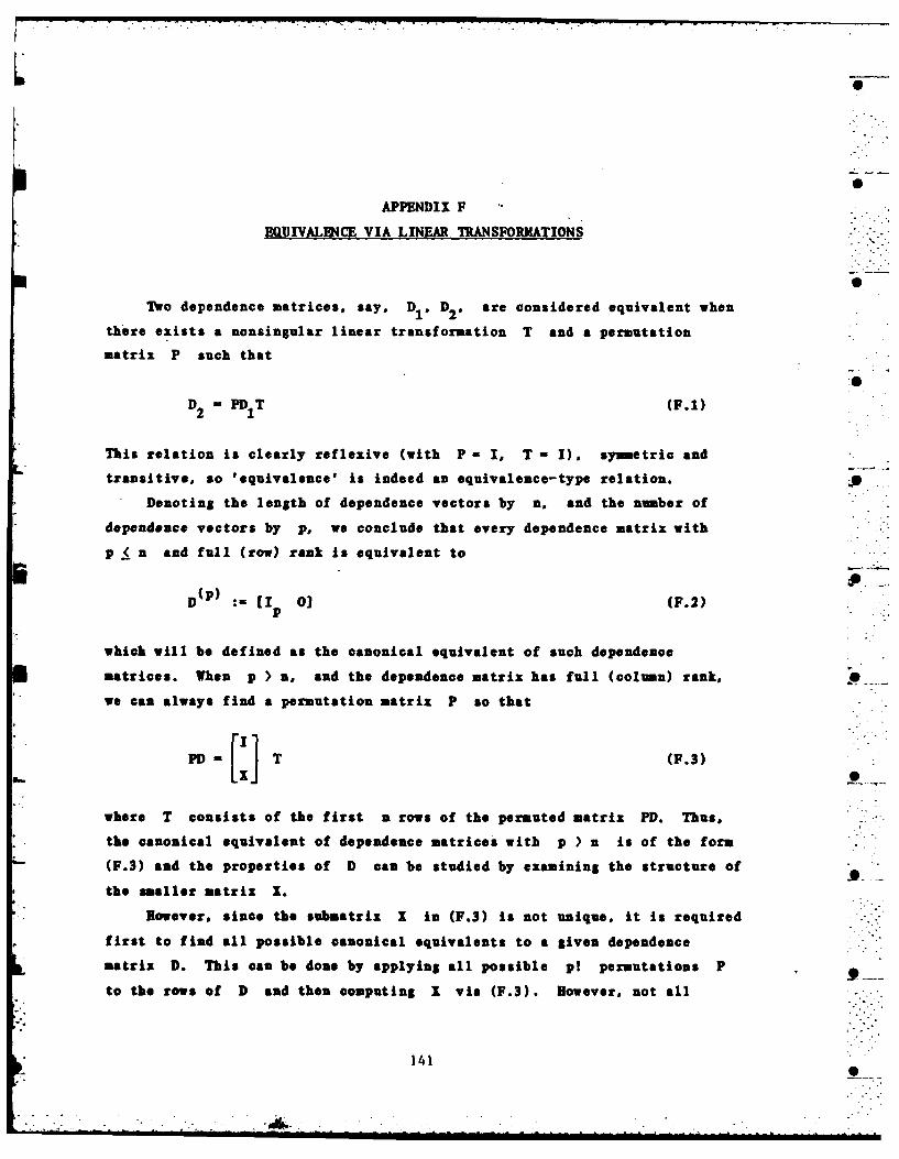
0
APPENDIX F
EQUIVALH4CE VIA LINEAR TRANSFORMATIONS
Two dependence matrices, say, D1 , D2, are considered equivalent when
there exists a nonsingular linear transformation T and a permutation
matrix P such that
D2 = PDIT (F.1)
This relation is clearly reflexive (with P = I, T I). symmetric and
transitive, so 'equivalence' is indeed an equivalence-type relation.
*Denoting the length of dependence vectors by n, and the number of
dependence vectors by p, we conclude that every dependence matrix with
p n and full (row) rank is equivalent to
D : W ( 0[ ] (F.2)p
which will be defined as the canonical equivalent of such dependence
matrices. When p > n. and the dependence matrix has full (column) rank, _
we can always find a permutation matrix P so that
PD = T (F.3) _
where T consists of the first n rows of the permuted matrix PD. Thus,
the canonical equivalent of dependence matrices with p ) n is of the form
(F.3) and the properties of D can be studied by examining the structure of
the smaller matrix X.
However, since the submatrix X in (F.3) is not unique, it is required
first to find all possible canonical equivalents to a given dependence
matrix D. This can be done by applying all possible pl permutations P -
to the rows of D and then computing I via (F.3). However, not all
141

In summary, once all possible canonical equivalents of a given D have -
been computed it is relatively easy to test whether some other dependence
matrix D is equivalent to D. One only needs to compute a single 0
canonical equivalent of D and compare it to the collection of canonical
equivalents of D: a match indicates that D is indeed equivalent to D. -I
14I
• __

L 129
10-84
DTI0