VHDL User Forum Europe, Dresden, 5.-8. May 1996, pp 85-96

Methodical Aspects of VHDL-based Field Bus Modelling with a Controller Area Network

Sven Altmann, Ulrich DonathFraunhofer-Institut für Integrierte Schaltungen,

Zeunerstr. 38, D 01069 Dresden

AbstractMethodical aspects are described to develop VHDL models of field bus systems. Field bus sys-tems used in automatic control engineering are examples of distributed computing systems.Modelling of such a system is demonstrated with a Controller Area Network (CAN). The con-sideration ranges from the process to the control devices. Targets are functional verificationsas well as performance predictions. Since the bus is a decisive component modelling is focusedon questions concerning the signal abstraction and the protocol used. VHDL code formulationis based on Statecharts. A design and simulation environment including the Synopsys VHDLsimulator is presented.

1 Introduction

Field buses considered here are communication media between components of distributedautomation systems [1]. In terminology of automatic control engineering, they are installed onthe lowest level of the automation hierarchy; i.e. they connect sensors, actuators, and controldevices to control a process. For modelling field bus systems, different approaches are appliedsuch as Queueing Networks [2] or Coloured Petri Nets [3]. These approaches consider thedevices or instruments as abstract service stations with mean arrival rates and service rates ortimes, respectively. However, function and performance of complex systems are determined bya variety of influence variables, e.g. by network structure, service types, priorities, responsetimes of application programs, load-dependent adjustments, and data-dependent function set-tings. So a more general approach is needed that takes into account the bus activity and thebehaviour of the subsystems connected by the bus. For modelling digital systems, VHDL hasproved to be an expressive and effective means. Therefore, VHDL is chosen to model field bussystems as well. Simulation on this basis allows to verify the design of the components and, onthe other hand, to predict performance features such as latency or response times. A ControllerArea Network (CAN) is applied to illustrate the methodical aspects. More generally speaking,the task belongs to the field of modelling parallel processes. The main idea consists in utilizingVHDL features for covering concurrency and hierarchy. If both time adjustments and trans-ferred data items are taken into account a combined simulation can be achieved showing per-formance and function of complex systems. In the near future, VHDL will be extended toanalog domain so that analog signal processing devices can be incorporated.

2 System View

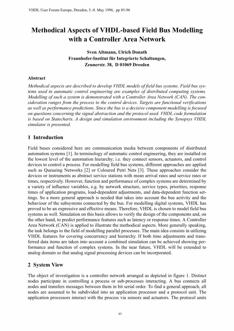
The object of investigation is a controller network arranged as depicted in figure 1. Distinctnodes participate in controlling a process or sub-processes interacting. A bus connects allnodes and transfers messages between them in bit serial order. To find a general approach, allnodes are assumed to be subdivided into an application processor and a protocol unit. Theapplication processors interact with the process via sensors and actuators. The protocol units

85

access the bus to send or receive data. While the application processors treat data according todifferent programs, the protocol units realize the same protocol.

Figure 1. System view of a contoller network1

Concerning the CAN technique, the following features are given [2][4][5]:ï Protocol: International Standard ISO 11519-1 and ISO 11519-2ï Multi-master systemï Medium access: CSMA/CD (Carrier Sense Multiple Access / Collision Detection)

+ AMP (Arbitration on Message Priority)ï Multicast message transferï Message identifiers determine their prioritiesï Acceptance filtering by the receiverï Data transfer service and remote data request serviceï Data length: 0 - 8 Byteï Bit rate: 10 - 1000 KBit/sï Error detection and error signalling.

As depicted in figure 1, the VHDL model of the system will be composed with the componentsProcess, Sensor, Actuator, and Node. The component Node is divided into the sub-componentsApplication Processor and Protocol Unit. In terms of VHDL, the transmission medium Buswill be modelled as a Resolved Signal driven by a Resolution Function. The signal flow direc-tions are shown in figure 1, too. First of all, the signal types have to be declared to achieve theinterface descriptions of the components and to set up the basis of component modelling.

1) µP - Microprocessor, PID - Proportional-Integral-Derivative Element

ApplµP

ProtUnitA

ApplµP

ProtUnitA

ApplµP

ProtUnitS

ProtUnit

APID- Process

S

Appl µP

ApplµP

ProtUnit S

Process

Sub-

Protocol Unit

Application µP

Bus

Node

Node

Node

Node

Node

Node

Sensor

Actuator

86

3 Bus and Protocol Units

3.1 Signal abstraction

In accordance with the Open Systems Interconnection (OSI) Reference Model, the CAN con-troller is organized hierarchically in the Data Link Layer and the Physical Layer, see figure 2.In the approach chosen, the Protocol Unit behaviourally performs the tasks of the Data LinkLayer as defined in the ISO Standard. The Physical Layer specifies an electrical circuit realiza-tion that connects the node to the bus. Since electrical features are not significant for behav-ioural modelling, this specification is not included.

Figure 2. Layers of the CAN Protocol

The Logical Link Control offers two services to its user: Data Transfer and Remote DataRequest. The data transfer service carries only a data frame from a transmitter to a receiver,whereas the remote data request service transmits a remote frame to a receiver to request a dataframe from this node. Figure 3 shows in which manner the contents of a data frame will beextended and arranged if a message passes from the Logical Link Control to the MediumAccess Control. Omitting the data field, a remote data request is equal to a data transfer.

Figure 3. Structure of the data frames

In order to declare the Resolved Signal, a unique signal type has to be defined. Therefore, theMAC data frame is chosen and adapted so that various tasks can be fulfilled:ï The Start Of Frame (SOF) bit marks the bus out as busy with a dominant ’0’. ï Data frames and remote frames are distinguished by the Remote Transmission Request

(RTR) bit with ’0’ or ’1’. ï The Control field gets the Data Length Code (DLC) from the LLC frame, but the Data field

itself is fixed to 8 bytes. ï If a remote frame is sent the Data field will be empty. ï The Identifier field, the CRC field, and the ACK field are kept up, whereas the End Of

Frame (EOF) mark is omitted. ï A time stamp is added to allow time measuring and event handling.

The result is a record type declared in the following type definition:

Application

Data LinkLayer

Logical Link Control (LLC)

Medium Access Control (MAC)

Physical Layer

Identifier DLC Data

Identifier DataSOF CRC ACKRTR Control EOF

LLC Layer

MAC Layer

1 Bit 11 Bit 1 Bit 6 Bit 0 - 8 Byte 16 Bit 2 Bit 10 Bit

87

TYPE bit_array IS ARRAY (0 TO 7) OF bit_vector(7 DOWNTO 0);

TYPE telegram IS RECORDsof: bit;identifier: integer;rtr: bit;control: integer;data: bit_array;crc: integer;ack: bit;stamp: time;

END RECORD;

According to the ISO standard, any node may start to transmit a frame when the bus turns idle.A conflict will arise if two or more nodes start the transmission at the same time. In this case,an arbitration mechanism uses the signal identifiers to solve the conflict. The identifiers arepositive integers having inverse priority, i.e. the identifier zero has the highest priority. Thetransmitter with the frame of highest priority gains the bus.

This arbitration is realized by the Bus Resolution Function, which checks all signal drivers ona dominant Start Of Frame. Comparison of the signal identifiers is carried out numerically, notbitwise. This is worth mentioning since the Bus Resolution Function significantly influencesthe simulation efficiency. For the same reason, the frames are transferred as a whole, not in asequence of data items.

3.2 Specification of control activities with Statecharts

Statecharts are applied to specify the control activities of the Protocol Unit. The subdivision ofthe Data Link Layer into Logical Link Control and Medium Access Control are taken from theISO Standard. Harel’s rules [6] are used to define the state transitions and to decompose thestates into substates. The schematic entry can be done with the ExpressV-HDL tool [7].

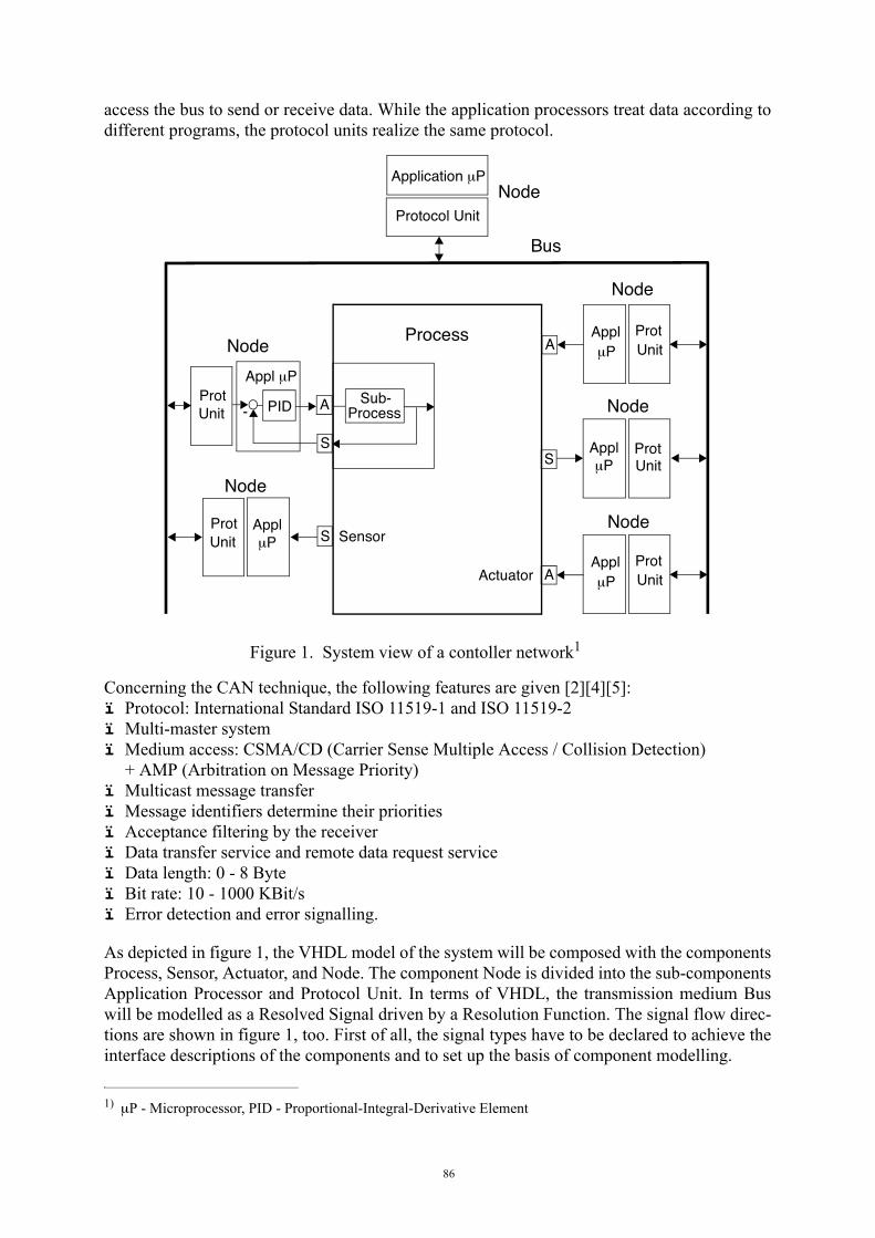
Figure 4. Representation of states and state transitions in Statecharts

Rounded boxes represent states, directed arcs symbolize state transitions. The general syntaxof an expression labelling a state transition is shown in figure 4. This expression may be readas follows: when the source state is marked and Event occurs and Condition is true then a tran-sition is carried out from the source state to the target state. Doing this Action is carried out. Inthe following, Events are signal changes or timeouts, Conditions are logical relations, andActions are signal assignments or procedure calls. If several actions have to be done they areseparated by semicolons.

Decomposition of states into substates is demonstrated with the top level chart of the MediumAccess Control, see figure 5.

Event [ Condition ] / Action

Start

State BState A

88

With respect to the fault management a node may be in one of the three states: Error Active,Error Passive, or Bus Off. A Transmit Error Counter and a Receive Error Counter, whichbelong to every node, determine the transitions among these states. Only in the Bus Off state anode is completely decoupled from the bus. The normal working state is the Error Active state.This state will be achieved after initialization or occurrence of a Restart event and will be left ifa Go Passive event is produced internally. The prefix @ of a state identifier indicates a refer-ence chart underlying.

Figure 5. Top Level Statechart of MAC

The Error Active state, see figure 6, is decomposed into four states: Ready, Send, Receive, andError. The initial state is Ready. Send is considered here for instance. Preconditions to enterSend are the following: Ready is marked, a data frame or remote frame has to be transmitted,and the bus is free. Send will be quitted if one of the events Go Receive, Send OK, or SendError is produced internally. The control activities for sending are represented in an additionalchart.

Figure 6. Error Active Statechart

Restart / execute_initialization

/ execute_initialization

@BusOff

@ErrorActive @ErrorPassive

GoBusOff

GoPassive

GoActive

/ execute_shutdown

MAC

Start

Ready

@Send @Receive

@Error

GoReceive / DataIn := False

SendOK /

[ DataIn and BusFree ]

Bus /BusFree := False

ReceiveOK /

SendError /update_error_count update_error_count

ReceiveError /

LLC_Request [ not DataIn ] /encapsulate_data;DataIn := True

BusFree := True

ErrorOver / BusFree := TrueExitErrorActive /

GoPassiveBusFree := True;

DataIn := False; decapsulate_data;BusFree := True

ErrorActive

89

The first function performed after entering Send is the data transmission, see figure 7. Thatmeans, the data frame is assigned to the bus port. After that, the arbitration will be checked tofind out whether the node gains the bus or not. In case the arbitration is lost the Go Receiveevent will be generated. If the node gains the bus, i.e. if the Arbitration OK event is generated,the time slot awaiting the acknowledgement will be computed. Then the Wait On ACK statewill be entered. This state will be left if the acknowledgement arrives or a Timeout eventoccurs. The latter causes a Send Error event, which will be dealt with after leaving Send.

Figure 7. Send Statechart.

Further charts are not detailed here because they are decomposed in the same manner.

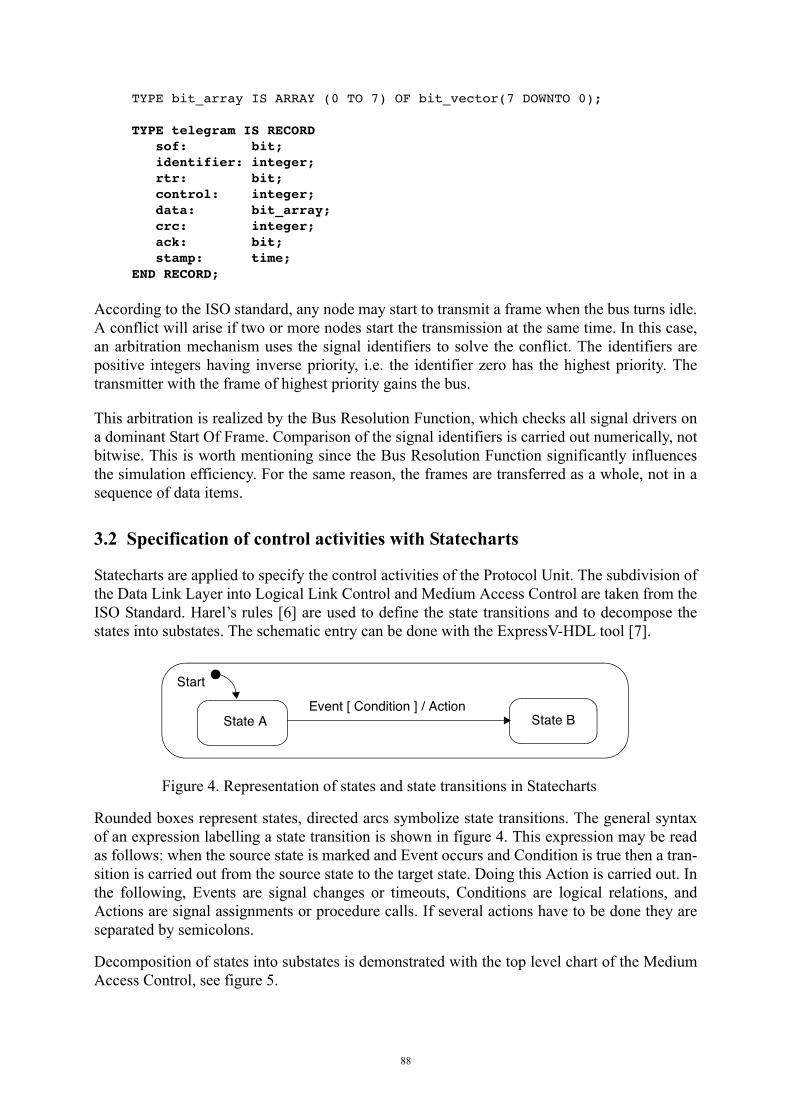
In figure 8, the time sequence diagram shows the interrelations between sender and receiverfor the case of an acknowledgement.

Having transmitted a telegram, the sender awaits either the acknowledgement or the timeout ofthe Receive ACK Timer. This timer is set to the expiry of the ACK time slot computed accord-ing to the number of bits transmitted until here and the bit time. In the model, the frames aretransferred without delay. So the receiver computes the time point for acknowledgement withthe same rule, but with the number of bits reduced by one. Without having achieved anacknowledgement, the sender transmits an error flag if the Receive ACK Timer expires. Bothsender and receiver adjust another timer - the EOF timer - to the remaining time interval of thetransmission phase. If these timers expire a new transmission can be started.

Regarding all timers in the instantiated nodes, the simulator yields the timing of the data trans-fer on the bus.

Transmit

@CheckArbitration

@WaitOnACK

SendEOF

/ BusFree := False; transmit_data

ArbitrationOK /ACK_Time := (36+DataLenght*8)*BitTime

Timeout ( entered ( WaitOnACK ), ACK_Time ) /SendError

Timeout ( entered (SendEOF), EOF_Time ) /

SendOK

ACK_Received /EOF_Time := 12*BitTime

ArbitrationLost /GoReceive

Send

turn_off;

90

Figure 8. Time sequence diagram of sender and receiver activities

3.3 VHDL code generation

The translation of Statecharts into VHDL code can be accomplished by the ExpressV-HDLtool [7] or manually. In order to get an optimal code for fast simulation, the manual translationwas preferred. Furthermore, functions for initialization, producing log-files, computing statis-tics, or any data processing can be added quickly if the VHDL code is well known.

The top level statecharts of the components are translated into design entities with correspond-ing architectural bodies. All reference charts are mapped into procedures called in the architec-tural body. As an example, the top level statechart of the MAC is considered.

The MAC entity declaration describes the interface to the Bus and to the Logical Link Control.Here, Bus is declared as a bidirectional signal of the type Telegram. The Telegram type decla-ration and all the other ones belong to the CAN package developed.

Besides signal declarations, the MAC architectural body contains a single Process statementincluding a Case statement and a Wait On statement. The Case statement specifies the statetransitions according to the Statechart representation in figure 5. Events in the Statechart aretranslated into signals with the attribute EVENT. The Wait On statement suspends the processuntil an event occurs related to its sensitivity list.

Translation of the MAC Statechart:

ENTITY CAN_MAC ISPORT ( Bus: INOUT Telegram; -- Bus interface

LLC_Request: IN LLC_Frame; -- LLC interfaceLLC_Indication: OUT LLC_Frame;LLC_Confirm: OUT LLC_Conf )

END CAN_MAC;

TelegramNode A Node B

Receive ACK Timer =(35+Data Length*8) * Bit Time

Send ACK Timer =

t

t

t CRC

t ACK

t

t

t SOF

t

AcknowledgementEOF Timer = EOF Timer =t

t

Timeout

(36+Data Length*8) * Bit Time

Telegram

12 * Bit Time

t t

Timeout

12 * Bit Time

EOF

DATA

ID

CONTROL

RTR

ACK

EOF

91

ARCHITECTURE behavioral OF CAN_MAC ISSIGNAL MacState: MacStateType := Start;SIGNAL GoPassive, GoActive, GoBusOff, Restart: bit;SIGNAL Toggle: bit;-- ...

BEGINCAN_MAC: PROCESSBEGIN

CASE MacState ISWHEN Start =>

-- ...WHEN ErrorActive =>

IF GoPassiveíEVENT THENMacState <= ErrorPassiv;

ELSEexecute_error_active; -- procedure call

END IF;WHEN ErrorPassive =>

-- ... WHEN BusOff =>

-- ...END CASE;

WAIT ONMacState, LLC_Request, Bus,GoPassive, GoActive, GoBusOff, Restart,Toggle;

END PROCESS;END behavioral;

All procedures detailing states have the same structure: a case statement specifies state transi-tions in dependency on EVENTs attributed to signals and/or logical relations. Any state transi-tion will be indicated by a Toggle event, which will affect the progress of the process via theWait On statement on the top level. In case a state has to be decomposed once more a furtherprocedure will be called with the structure just described.

4 Application processors, sensors, and actuators

The tasks usually placed in the CAN application layer are the following: ï polling of sensorsï transmission of polled valuesï transmission of events signalled by limit indicators ï data preprocessingï passing of set-point values to actuatorsï control settings.

In the model, these tasks will be performed by the application processors. Again, the VHDLdescription is formulated on behavioural level. For instance, a temperature control will be con-sidered with a Poll Processor and a Heating Controller.

The Poll Processor only inserts the given temperature value in a request frame and directs thisframe to its corresponding Protocol Unit. This is repeated isochronously according to a Wait

92

For statement adjusted to the required sample period. The signal identifier and the sampleperiod are read from a network configuration file during the initialization step.

ENTITY POLL_PROCESSOR IS GENERIC ( NodeNo: natural; -- node number ConfigFile: string ); -- configuration file

PORT ( Temperature: IN real; -- input from sensorIndication: IN LLC_Frame; -- input from protocol unitConfirm: IN LLC_Conf; -- input from protocol unitRequest: OUT LLC_Frame ) -- output to protocol unit

END POLL_PROCESSOR;

ARCHITECTURE behavioral OF POLL_PROCESSOR ISBEGIN PROCESS VARIABLE Init: bit; SignalID: integer; Period: time; BEGIN IF NOT Init THEN read_config_file ( NodeNo, ConfigFile, SignalID, Period ); Init := í1í; END IF; WAIT FOR Period; Request <= real_to_frame ( SignalID, Temperature ); END PROCESS;END;

The Heating Controller receives the temperature value as part of an indication frame from theProtocol Unit coupled. In dependency on the range settings, the control signal Heating isassigned to ’1’ or ’0’. This operation will be repeated if a new indication occurs.

ENTITY HEATING_CONTROLLER ISGENERIC ( NodeNo: natural; -- node number

ConfigFile: string ); -- configuration filePORT ( Heating: OUT bit; -- output to actuator

Indication: IN LLC_Frame; -- input from protocol unitConfirm: IN LLC_Conf; -- input from protocol unitRequest: OUT LLC_Frame ) -- output to protocol unit

END HEATING_CONTROLLER;

ARCHITECTURE behavioral OF HEATING_CONTROLLER ISBEGIN PROCESS VARIABLE Init: bit; SignalID: integer; VARIABLE Temperature, LowTemp, HighTemp: real; BEGIN IF NOT Init THEN

read_config_file (NodeNo, ConfigFile, SignalID, LowTemp, HighTemp);Init := í1í;

END IF; WAIT ON Indication; Temperature := frame_to_real ( SignalID, Indication ); IF Temperature < LowTemp THEN Heating <= í1í; ELSIF Temperature > HighTemp THEN Heating <= í0í; END IF; END PROCESS;END;

93

Sensors and actuators are also modelled in this way. If a process model is available signals willbe sent to or received from this model. The signals may be typified in any kind or composition.With the sampling method, for instance, a discrete-time model of the process can be created[8]. In the near future, analog extensions of VHDL (VHDL-A) will allow to incorporate con-tinuous process models. However, if a process model is not available signal sequences have tobe obtained by reading files containing test patterns or utilizing approximation functions. Ifonly a traffic load has to be produced sensors and application processors will be replaced byevent generators. These generators issue telegrams in isochronously, uniformly, or exponen-tially distributed periods, the latter ones are quantified.

5 Simulation

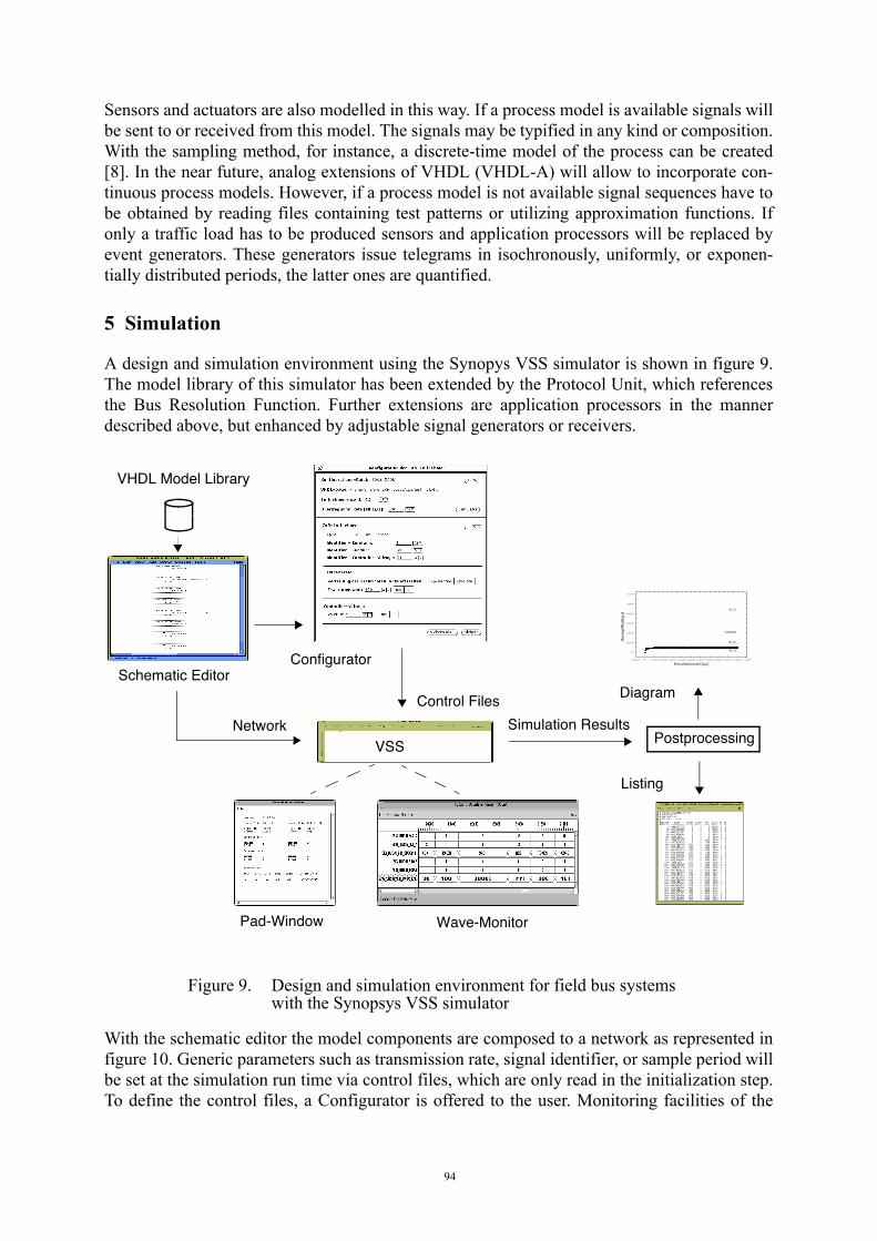
A design and simulation environment using the Synopys VSS simulator is shown in figure 9.The model library of this simulator has been extended by the Protocol Unit, which referencesthe Bus Resolution Function. Further extensions are application processors in the mannerdescribed above, but enhanced by adjustable signal generators or receivers.

Figure 9. Design and simulation environment for field bus systems with the Synopsys VSS simulator

With the schematic editor the model components are composed to a network as represented infigure 10. Generic parameters such as transmission rate, signal identifier, or sample period willbe set at the simulation run time via control files, which are only read in the initialization step.To define the control files, a Configurator is offered to the user. Monitoring facilities of the

-1 ,0 x1 0 5 0 ,0 1 ,0 x10 5 2 ,0x1 0 5 3 ,0 x1 0 5 4 ,0 x10 5 5 ,0x1 0 5 6 ,0 x1 0 5 7 ,0 x1 0 5 8 ,0 x1 0 5 9 ,0 x1 0 5 1 ,0x1 0 6 1 ,1 x1 0 6

0 ,0

2 ,0 x10 2

4 ,0 x10 2

6 ,0 x10 2

8 ,0 x10 2

1 ,0 x10 3

1 ,2 x10 3

ID_72

Controller

ID_12

ID_10

Busz

ugrif

fsze

it [µ

s]

Sim ulationszeit [µs ]ConfiguratorSchematic Editor

Control Files

VHDL Model Library

NetworkVSS Postprocessing

Simulation Results

Diagram

Listing

Pad-Window Wave-Monitor

94

simulator are applied to depict the traffic or to report lost data. The Wave Monitor shows themessages on the transmission medium in their timing. Details referring to occupied buffers,latent periods, response times, or lost data are directed to the Pad Window. The system isextended by a Bus Observer which writes selected data or events into a log-file. Similar reportscan be produced by the Protocol Unit, too. The analysis of these data items is done in a post-processing step with various programs.

Figure 10. Composition of a controller network

Simulation experiments have been carried out with different systems using CAN-Bus, PROFI-BUS, or INTERBUS-S. For the latter ones, equivalent simulation environments were installed.

With the CAN simulation, the medium access times of a sensor/actuator system consisting of12 participants were determined. Figure 11 and figure 12 show the simulation results. Here, themedium access time is the time interval between generating a message and its complete trans-mission.

Figure 11. Mean medium access times of the CAN example

Application X

ProtocolUnit

Node X

Application Y

ProtocolUnit

Node YApplication Z

ProtocolUnit

BUS

ID_72

Controller

ID_12

ID_10ID = 10

ID = 12

ID = 72

Controller

mea

n m

ediu

m a

cces

s tim

e / m

s

1.0

0.8

0.6

0.4

0.2

0

0 10.5

1.2

simulated real time / s

95

Figure 12. Mean value and current values of the medium access time of a CAN node

In the CAN example, the sensors transmit broadcasts in isochronously or exponentially distrib-uted periods. The receivers and actuators, respectively, select the messages according to theidentifiers given to them. Among the participants, a controller periodically transmits a remoteframe to all other nodes to request data.

Figure 11 shows the development of the mean medium access times during 1s simulated realtime with the bit rate of 500 KBit/s. The controller curve represents a set of signals since thecontroller sends broadcasts with various priorities. For this simulation 6.5 min CPU timeelapsed on a Sun Sparc 10 station. Figure 12 shows the relations between the mean value andthe current values of the medium access time of single node. The peaks illustrate the need ofdetailed investigations in time critical applications.

References

[1] Arnold, M.: Feldbussysteme. ELRAD 1993.Teil 1, Heft 4, S.56-60. Teil 2, Heft 5, S.79-81

[2] Lawrenz, W.[Hrsg]: CAN Controller Area Network: Grundlagen und Praxis. Hüthig,Heidelberg, 1994

[3] Kiefer, J.: Methodischer Entwurf von Feldbussystemen in der Automatisierungstechnik.4.Tagung "Entwurf komplexer Automatisierungssysteme", Braunschweig, Juni 1995, S. 521-541,

[4] ISO 11519-2: Road Vehicles - Low Speed Serial Data communication - Controller AreaNetwork (CAN). 1994

[5] Bonfig, K.W. et al: Feldbus Systeme. expert verlag, Renningen-Malmsheim, 1995

[6] Harel, D. et al: STATEMATE: A Working Environment for the Development of ComplexReactive Systems. IEEE Transactions on Software Engineering, Vol. 16, April 1990, pp. 403-413

[7] i-Logix Inc: Express V-HDL. Version 3.0 Documentation. Andover MA, 1993

[8] Donath, U.: Schnittstellen für Modelle in KOSIM und Lsim. Workshop "Modellierungund Simulation in der Nachrichtentechnik", Dresden, November 1995

simulated real time / s0 0.5 1

med

ium

acc

ess

time

/ ms

1.0

0.8

0.6

0.4

0.2

0

mean value

current values

96