Method of Characteristics and Numerical Solutions for the Supersonic External Ballistics Problem

Method of Characteristics and Numerical Solutions for the

Supersonic External Ballistics Problem

by

Keith D. Smith

A Thesis Submitted to the Graduate

Faculty of Rensselaer Polytechnic Institute

in Partial Fulfillment of the

Requirements for the degree of

MASTER OF ENGINEERING

2nd

Complete Draft

17 July 09

Approved:

_________________________________________

Dr. David Tew, Thesis Adviser

_________________________________________

Dr. Ernesto Gutierrez-Miravete, Thesis Adviser

Rensselaer Polytechnic Institute

Troy, New York

August 2009

1

© Copyright 2009

by

Keith D. Smith

All Rights Reserved

2

CONTENTS

LIST OF TABLES............................................................................................................. 4

LIST OF FIGURES ........................................................................................................... 5

NOMENCLATURE .......................................................................................................... 6

ACKNOWLEDGMENT ................................................................................................... 8

ABSTRACT ...................................................................................................................... 9

1. Introduction................................................................................................................ 10

1.1 General External Ballistics............................................................................... 11

1.1.1 Projectile Features................................................................................ 11

1.1.2 Flight Speeds........................................................................................ 14

1.2 Problem Definition........................................................................................... 15

1.2.1 Description ........................................................................................... 15

1.2.2 Assumptions......................................................................................... 17

1.3 Governing Equations........................................................................................ 18

1.3.1 Conservation of Mass........................................................................... 18

1.3.2 Conservation of Momentum ................................................................ 19

1.3.3 Conservation of Energy........................................................................ 20

1.3.4 Method of Characteristics Velocity Potential Form ............................ 21

1.3.5 Finite Volume Numerical Method Form ............................................. 21

2. Methodology.............................................................................................................. 22

2.1 Reynolds Number ............................................................................................ 22

2.2 Method of Characteristics ................................................................................ 23

2.2.1 Process.. ............................................................................................... 23

2.2.2 Equations.............................................................................................. 28

2.3 Numerical Method ........................................................................................... 30

2.3.1 Mesh Generation .................................................................................. 31

2.3.2 Fluent® Implementation ...................................................................... 34

3

3. Results and Discussion .............................................................................................. 39

3.1 Experimental Illustration.................................................................................. 39

3.2 Quantitative Comparisons................................................................................ 41

3.3 Qualitative Comparisons.................................................................................. 48

3.3.1 Coarse Mesh......................................................................................... 48

3.3.2 Medium Mesh ...................................................................................... 51

3.3.3 Fine Mesh............................................................................................. 54

3.3.4 Drag Coefficient................................................................................... 58

4. Conclusions................................................................................................................ 60

5. Areas for Future Work............................................................................................... 62

6. References.................................................................................................................. 63

4

LIST OF TABLES

Table 1-1: Representative Projectile Muzzle Velocities ................................................. 15

Table 2-1: Mesh Grid Summary ...................................................................................... 33

Table 3-1: Minimum Mach number Comparison............................................................ 44

Table 3-2: Drag Coefficient Comparison ........................................................................ 59

5

LIST OF FIGURES

Figure 1-1: General Projectile Features ........................................................................... 11

Figure 1-2: Base Drag Force Reduction Features Overview........................................... 13

Figure 1-3: NACA No. 24 Projectile Dimensions........................................................... 16

Figure 2-1: Method of Characteristics Physical Plane .................................................... 23

Figure 2-2: Location of the Shock Front ......................................................................... 24

Figure 2-3: Partition of the Physical Plane ...................................................................... 25

Figure 2-4: Characteristic Net and Intersection Points.................................................... 27

Figure 2-5: Physical Plane Mesh ..................................................................................... 32

Figure 2-6: Coarse Mesh Grid ......................................................................................... 33

Figure 3-1: Schlieren Illustration for a NACA 1122 No. 32 Shape (w/Boat Tail).......... 40

Figure 3-2: Verification of Shock Attachment ................................................................ 42

Figure 3-3: Mach number Comparison Immediately Downstream of Shock Front ........ 43

Figure 3-4: Projectile Surface Mach number Comparison .............................................. 45

Figure 3-5: Method of Characteristics Projectile Surface Pressure Ratio ....................... 46

Figure 3-6: Numerical Model Pressure Ratio .................................................................. 47

Figure 3-7: Coarse Mesh Static Mach number Contour Map.......................................... 49

Figure 3-8: Coarse Mesh Mach number Surface Map..................................................... 49

Figure 3-9: Coarse Mesh Pressure Contour Map ............................................................ 50

Figure 3-10: Coarse Mesh Pressure Surface Map ........................................................... 51

Figure 3-11: Medium Mesh Mach number Contour Map ............................................... 52

Figure 3-12: Medium Mesh Mach number Surface Map ................................................ 52

Figure 3-13: Medium Mesh Static Pressure Contour Map.............................................. 53

Figure 3-14: Medium Mesh Static Pressure Surface Map............................................... 54

Figure 3-15: Fine Mesh Mach number Contour Map...................................................... 55

Figure 3-16: Fine Mesh Velocity Surface Map ............................................................... 55

Figure 3-17: Fine Mesh Static Pressure Contour Map .................................................... 56

Figure 3-18: Fine Mesh Static Pressure Surface Map ..................................................... 57

Figure 3-19: Shock Attachment to the Projectile Nose, Mach number........................... 57

Figure 3-20: Shock Attachment to the Projectile Nose, Static Pressure.......................... 58

6

NOMENCLATURE

ρ - fluid density

t - time

u - velocity vector (u = ux î + ur ĵ)

r - r-coordinate distance

x - x-coordinate distance

Sm - fluid mass source term (for combustion)

g - gravitational vector (constant)

p - static pressure

p0 - total or stagnation pressure

F - external force vector

Et - total energy

hj - diffusion energy term (see Fluent®)

Jj - diffusion energy term (see Fluent®)

Sh - volumetric energy source term (for chemical reactions)

Φ - velocity potential function

a - sound speed

V - volume

A - area

H - enthalpy

τxi - viscous term

τri - viscous term

τij - viscous term

q - heat flux

Re - Reynolds number

l0 - characteristic length

v0 - characteristic velocity

µ0 - fluid viscosity

θ - turn angle

θnose - projectile nose tangent angle

7

NOMENCLATURE

θshock - shock front angle

θfan - projectile base forward expansion fan Mach line angle

α - flight angle of attack

µ - Mach angle

β - local Mach angle

ν - Prandtl-Meyer angle

γ - fluid specific heat ratio

Cd - drag coefficient

8

ACKNOWLEDGMENT

9

ABSTRACT

The external ballistics problem has been studied for several decades in an effort to

improve flight range or optimize projectiles for a given mission scenario. This paper

considers the specific problem of unpowered supersonic flight of a simple axi-symmetric

shape such as a bullet or artillery shell. The objective is to compare two calculation

methods that offer an Euler solution to the velocity and pressure field characteristics near

the projectile. The problem is simplified to inviscid steady-state conditions.

An analytic solution is obtained using the Method of Characteristics (MoC) ap-

proach that encompasses the Euler equations in a single second order differential

equation using the velocity potential function. The second solution is provided by a

finite volume numerical method that solves the Euler equations in coupled vector form.

The comparisons show that both methods capture the shape and oblique angle char-

acteristics of the projectile nose shock. However, the MoC solutions do not indicate

vorticity across the shock due to the application of additional isentropic fluid assump-

tions. The numerical solutions included vorticity as indicated by the curvature of the

shock front, but did not adequately represent the fluid gradients across the shock front

for the three mesh densities that were evaluated. Though it was not the principal focus of

this paper, the numerical solutions also provided a drag coefficient that was only 4%

lower than previously reported experimental data even though viscous effects were

neglected.

10

1. Introduction

The external ballistics problem has been studied for several decades in an effort to

improve flight range or optimize projectiles for a given mission scenario. This paper

considers the specific problem of unpowered supersonic flight of a simple axi-symmetric

shape such as a bullet or artillery shell. The objective is to compare two calculation

methods that offer an Euler solution to the velocity and pressure field characteristics near

the projectile. The problem is simplified to inviscid steady-state conditions. The topic

was chosen based on an introduction to the subject presented in Anderson [1].

An analytic solution is obtained using the Method of Characteristics (MoC) ap-

proach that encompasses the Euler equations in a single second order differential

equation using the velocity potential function. The second solution is provided by a

finite volume numerical method that solves the Euler equations in coupled vector form.

Both methods solve Euler’s equations for continuity (conservation of mass), conserva-

tion of momentum and conservation of energy assuming inviscid flow.

Supersonic projectile motion has been extensively studied in a variety of applica-

tions ranging from small arms and artillery projectiles to missiles and manned

supersonic aircraft. The flow fields around the projectile are a function of the fluid

thermodynamic properties, its flight speed and shape. The ability to accurately quantify

the fluid behavior near a projectile in flight is important for determining the flight

characteristics. High velocity and pressure gradients will occur near shock or expansion

(sometimes called rarefaction) waves affecting flight characteristics such as drag force,

lift force or projectile center of pressure. In many applications, lower drag force is

sought to enable higher projectile speeds, increased range, improved propulsion effi-

ciency or an optimized design for a given mission.

This paper examines characteristics of the fluid velocity and pressure field for a spe-

cific external ballistics case of a simple axi-symmetric projectile. The problem is

restricted to the scale of small arms or artillery scale projectiles. Characteristics of

interest include the position and strength of shock fronts, the formation of expansion

regions (or rarefaction waves), Mach angle at the projectile base, and the Mach speed at

the surface of the projectile. Flow characteristics occurring in the wake downstream of

the projectile base are not included in this study.

11

The following sections provide a general introduction to external ballistics problems

including terminology used to describe features and flight speeds. The general discus-

sion is followed by a detailed description of the topic problem and governing equations.

The methodology, results and conclusions are presented in later sections.

1.1 General External Ballistics

1.1.1 Projectile Features

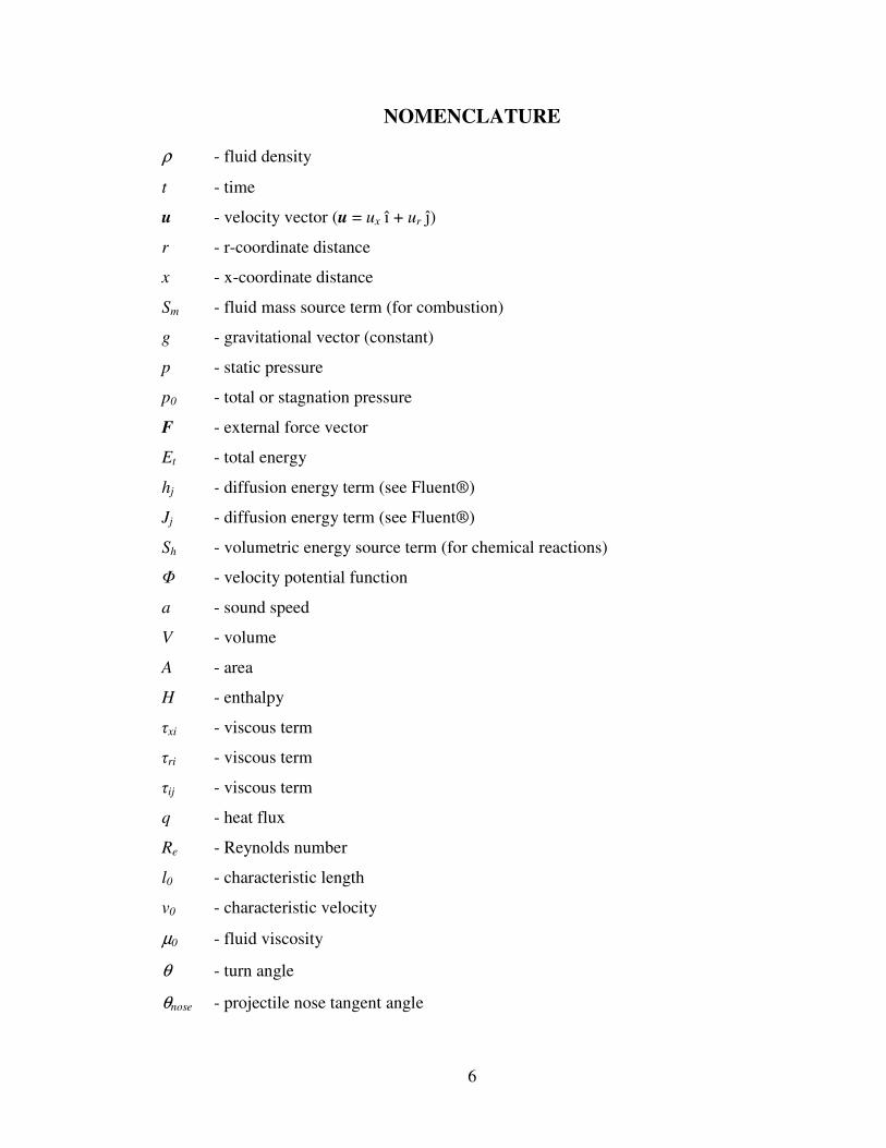
The National Advisory Committee for Aeronautics (NACA) studied a variety of

standardized missile shapes [2]. The primary features of these standard shapes are

illustrated in Figure 1-1 and accompanied by a brief introduction to terminology.

NACA Report 1122, Shape No. 24

Payload Area

Nose or Head

Ogive (pronounced “oh-jive”) Body

Base

(Image taken from Gambit® modeling utility)

Figure 1-1: General Projectile Features

Starting from the upwind direction on the left, the nose or head performs the initial

turn of the fluid field around the projectile. The sharpness of the nose determines the

attached or detached state of the shock while the inflow speed sets the shock angle

relative to the projectile axis. The nose is followed by a region of increasing cylindrical

radius called the ogive section (pronounced "Oh-jive," the term means a curved shape or

12

feature). The ogive can be conical appearing as a triangle in cross-section or it may be

represented by a conic section such as a circular, parabolic or elliptic arc. A tangent

ogive shape is simply any ogive shape that is tangent to the body cylinder at the intersec-

tion point. Simple axi-symmetric ogive shapes are often chosen for mass produced

projectiles such as bullets or model rockets whereas semi axi-symmetric shapes may be

preferred for larger scale objects such as fighter aircraft where cost is less of a considera-

tion.

The cylindrical section following the ogive is called the projectile body. The size of

the body has a significant affect on the projectile’s payload, center of gravity and the

development of a turbulent boundary layer. For ballistic shapes, the maximum diameter

of the body section is used as a reference dimension for all other projectile dimensions

and is expressed in caliber (measured in inches) or millimeters. By convention, the

decimal place is omitted from non-metric caliber sizes less than one inch (eg. 0.30 inch

diameter is denoted 30 caliber)

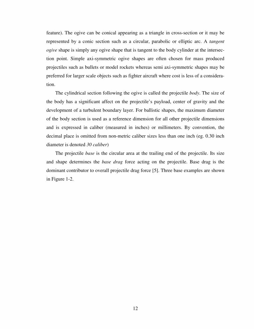
The projectile base is the circular area at the trailing end of the projectile. Its size

and shape determines the base drag force acting on the projectile. Base drag is the

dominant contributor to overall projectile drag force [5]. Three base examples are shown

in Figure 1-2.

13

Simple Base

Boat Tail

Boat Tail (7.5°to Axis)

Recessed Base Boat Tail

Figure 1-2: Base Drag Force Reduction Features Overview

The least complex base is represented by a flat circular area exhibiting the same di-

ameter at the projectile body. A tapered body section called a boat tail is employed in

some projectile designs to reduce base drag force. A boat tail angle between 6 and 9

degrees is considered optimum for a practical range of supersonic flight speeds [3].

Some projectiles implement both a boat tail and a hollow base to further reduce base

drag force [4]. The boat tails is detrimental to muzzle velocity because it provides an

efficient aerodynamic shape for high pressure fluid to flow around the projectile during

the transition from internal to external ballistic flight when the bullet leaves the gun

barrel. Some small arms projectiles further modify the boat tail to produce a step be-

tween the body and boat tail mitigating this effect. The stepped design is called a rebated

boat tail (not shown).

The overall projectile length affects flight stability and formation of the turbulent

boundary layer [2]. Flight stability refers to the steady orientation of the projectile

relative to its direction of travel. Further discussion of flight stability and turbulence are

beyond the scope of this study though extensive discussion is available in open litera-

ture.

14

1.1.2 Flight Speeds

In general, the speed of a projectile varies throughout its flight path or trajectory.

For unpowered projectiles, the rate of deceleration is inversely proportional to the cross-

sectional loading (the ratio of projectile weight to cross-sectional area) and directly

proportional to the drag coefficient [2]. By convention, the barrel exit or muzzle velocity

is used to represent the kinetic energy or initial speed regime for small arms and artillery

projectiles. Representative small arms muzzle velocities can range from Mach 1.2 to

Mach 3.7 for conventional projectiles, and may remain supersonic at practical ranges

(~200 yards) exhibiting speeds up to Mach 2.7 [7] [8]. Armor piercing and other spe-

cialty projectiles may achieve higher muzzle velocities [9]. A small sample of

representative small arms and artillery projectiles is presented in Table 1-1. The table

lists sizes expressed in base diameter (millimeters) and muzzle velocities from various

sources [7] [8] [9].

15

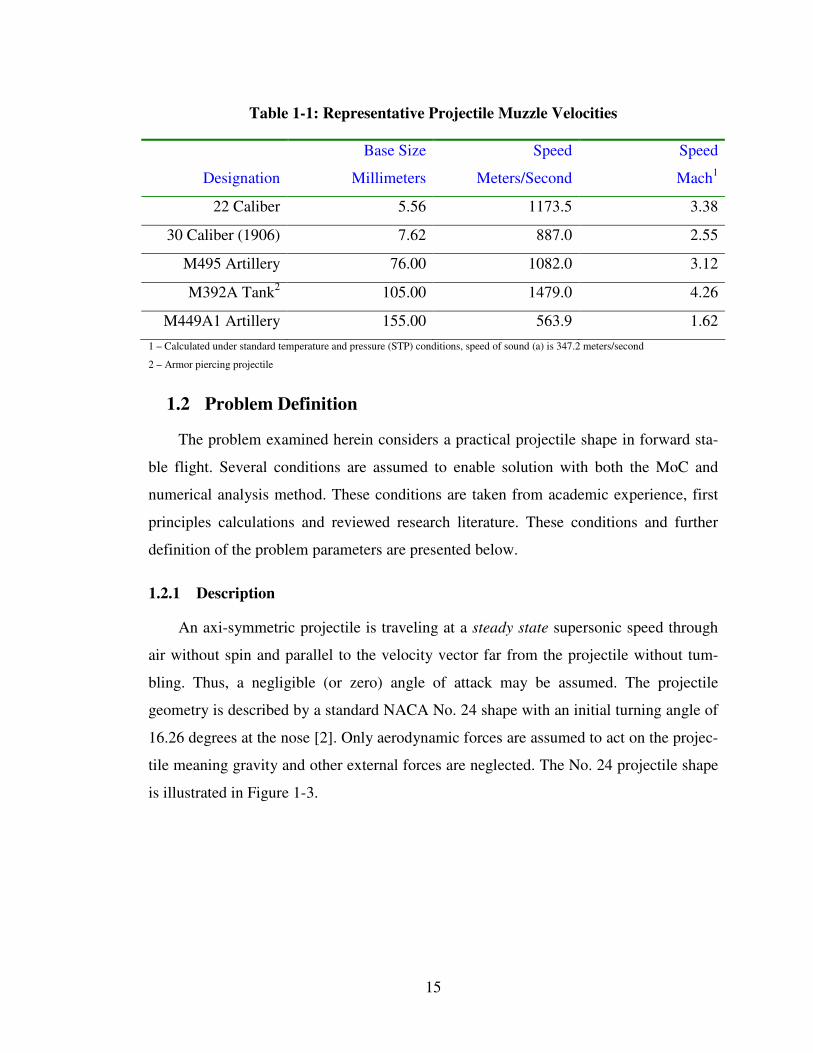
Table 1-1: Representative Projectile Muzzle Velocities

Designation

Base Size

Millimeters

Speed

Meters/Second

Speed

Mach1

22 Caliber 5.56 1173.5 3.38

30 Caliber (1906) 7.62 887.0 2.55

M495 Artillery 76.00 1082.0 3.12

M392A Tank2 105.00 1479.0 4.26

M449A1 Artillery 155.00 563.9 1.62

1 – Calculated under standard temperature and pressure (STP) conditions, speed of sound (a) is 347.2 meters/second

2 – Armor piercing projectile

1.2 Problem Definition

The problem examined herein considers a practical projectile shape in forward sta-

ble flight. Several conditions are assumed to enable solution with both the MoC and

numerical analysis method. These conditions are taken from academic experience, first

principles calculations and reviewed research literature. These conditions and further

definition of the problem parameters are presented below.

1.2.1 Description

An axi-symmetric projectile is traveling at a steady state supersonic speed through

air without spin and parallel to the velocity vector far from the projectile without tum-

bling. Thus, a negligible (or zero) angle of attack may be assumed. The projectile

geometry is described by a standard NACA No. 24 shape with an initial turning angle of

16.26 degrees at the nose [2]. Only aerodynamic forces are assumed to act on the projec-

tile meaning gravity and other external forces are neglected. The No. 24 projectile shape

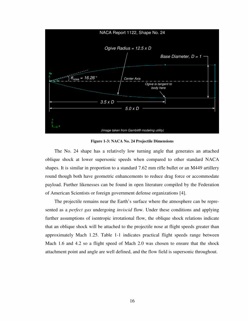
is illustrated in Figure 1-3.

16

NACA Report 1122, Shape No. 24

Ogive Radius = 12.5 x D

Base Diameter, D = 1

(Image taken from Gambit® modeling utility)

3.5 x D

5.0 x D

Ogive is tangent to body here

Center Axisθnose = 16.26°

Figure 1-3: NACA No. 24 Projectile Dimensions

The No. 24 shape has a relatively low turning angle that generates an attached

oblique shock at lower supersonic speeds when compared to other standard NACA

shapes. It is similar in proportion to a standard 7.62 mm rifle bullet or an M449 artillery

round though both have geometric enhancements to reduce drag force or accommodate

payload. Further likenesses can be found in open literature compiled by the Federation

of American Scientists or foreign government defense organizations [4].

The projectile remains near the Earth’s surface where the atmosphere can be repre-

sented as a perfect gas undergoing inviscid flow. Under these conditions and applying

further assumptions of isentropic irrotational flow, the oblique shock relations indicate

that an oblique shock will be attached to the projectile nose at flight speeds greater than

approximately Mach 1.25. Table 1-1 indicates practical flight speeds range between

Mach 1.6 and 4.2 so a flight speed of Mach 2.0 was chosen to ensure that the shock

attachment point and angle are well defined, and the flow field is supersonic throughout.

17

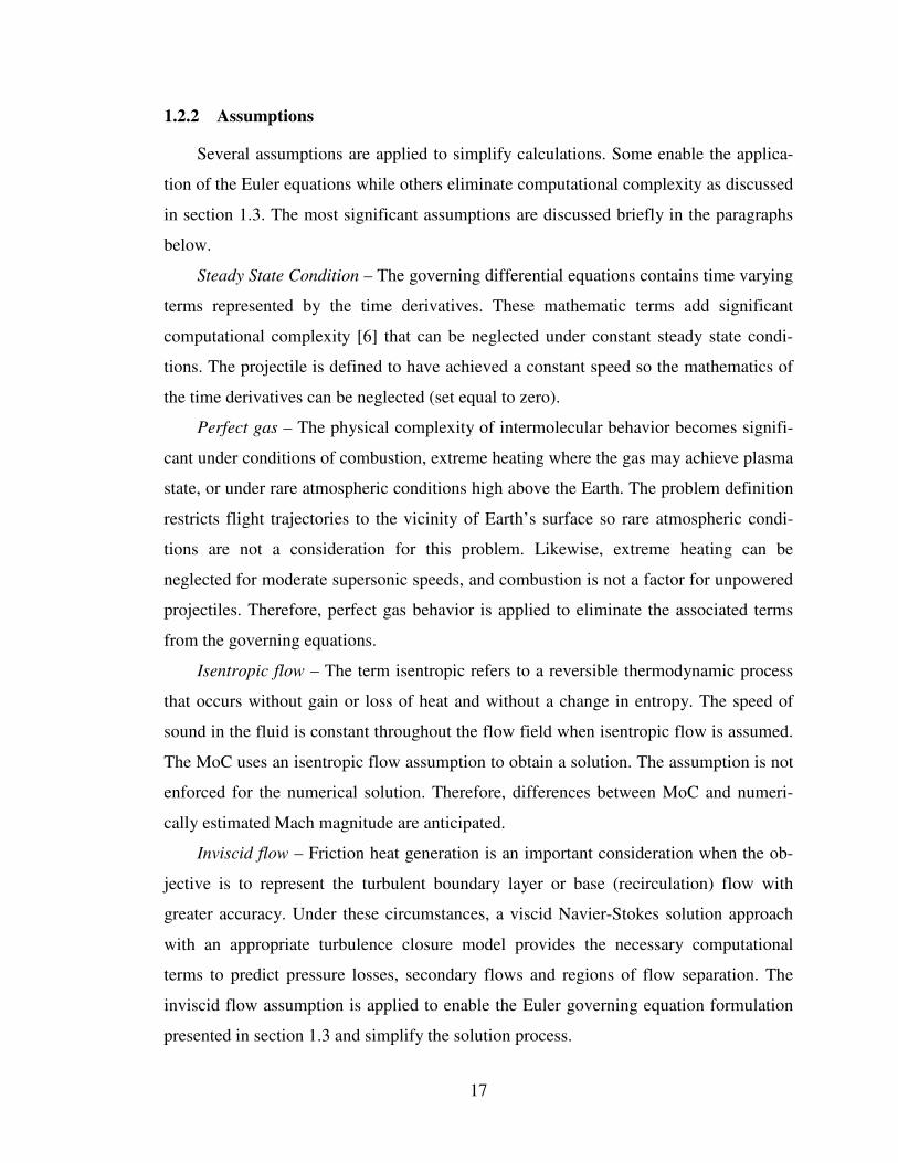
1.2.2 Assumptions

Several assumptions are applied to simplify calculations. Some enable the applica-

tion of the Euler equations while others eliminate computational complexity as discussed

in section 1.3. The most significant assumptions are discussed briefly in the paragraphs

below.

Steady State Condition – The governing differential equations contains time varying

terms represented by the time derivatives. These mathematic terms add significant

computational complexity [6] that can be neglected under constant steady state condi-

tions. The projectile is defined to have achieved a constant speed so the mathematics of

the time derivatives can be neglected (set equal to zero).

Perfect gas – The physical complexity of intermolecular behavior becomes signifi-

cant under conditions of combustion, extreme heating where the gas may achieve plasma

state, or under rare atmospheric conditions high above the Earth. The problem definition

restricts flight trajectories to the vicinity of Earth’s surface so rare atmospheric condi-

tions are not a consideration for this problem. Likewise, extreme heating can be

neglected for moderate supersonic speeds, and combustion is not a factor for unpowered

projectiles. Therefore, perfect gas behavior is applied to eliminate the associated terms

from the governing equations.

Isentropic flow – The term isentropic refers to a reversible thermodynamic process

that occurs without gain or loss of heat and without a change in entropy. The speed of

sound in the fluid is constant throughout the flow field when isentropic flow is assumed.

The MoC uses an isentropic flow assumption to obtain a solution. The assumption is not

enforced for the numerical solution. Therefore, differences between MoC and numeri-

cally estimated Mach magnitude are anticipated.

Inviscid flow – Friction heat generation is an important consideration when the ob-

jective is to represent the turbulent boundary layer or base (recirculation) flow with

greater accuracy. Under these circumstances, a viscid Navier-Stokes solution approach

with an appropriate turbulence closure model provides the necessary computational

terms to predict pressure losses, secondary flows and regions of flow separation. The

inviscid flow assumption is applied to enable the Euler governing equation formulation

presented in section 1.3 and simplify the solution process.

18

Irrotational flow – Rotational flow introduces a fluid point property called vorticity.

Vorticity causes the flow to change direction and occurs in fluid regions where high

enthalpy or entropy gradients occur (ie. around shock waves). It is observed as shock

curvature. The MoC assumes irrotational flow to obtain an analytic solution so estimated

shock waves will be straight. The irrotational flow assumption is not enforced in the

numerical method so curved shock wave are anticipated for these solutions.

1.3 Governing Equations

There are a number of valid sets of equations for modeling external ballistic prob-

lems. The Euler equations have been selected for this study because they can be solved

with both MoC and numerical calculation methods, and encompass enough of the

physics to estimate the flow fields near the projectile. The Euler equations permit

rotational flow and enthalpy losses through shock waves, and are very useful in solving

transonic flow problems, propeller or rotor aerodynamics, and flows with vortical

structures in the field. However, none of these capabilities will be explored during

solution of this problem.

The following sections present the equations for conservation of mass, momentum

and energy and provide comparisons to the equation forms used for the MoC calcula-

tions and by the Fluent® software application. The governing equations originate from

Anderson (Chapter 8), Tannehill (section 5.5) and the Fluent® User’s Manual [1] [10]

[11]. The notation has been adjusted to allow clear and consistent comparisons.

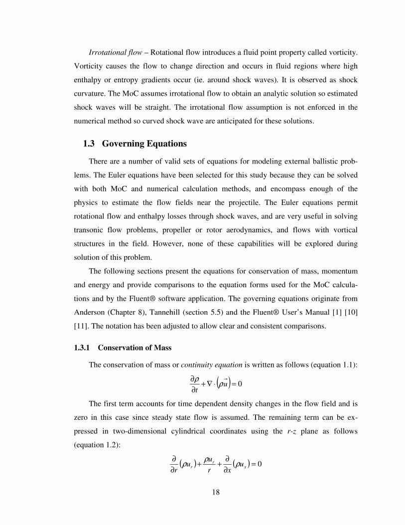
1.3.1 Conservation of Mass

The conservation of mass or continuity equation is written as follows (equation 1.1):

( ) 0=⋅∇+∂

∂u

tρ

ρ

The first term accounts for time dependent density changes in the flow field and is

zero in this case since steady state flow is assumed. The remaining term can be ex-

pressed in two-dimensional cylindrical coordinates using the r-z plane as follows

(equation 1.2):

( ) ( ) 0=∂

∂++

∂

∂x

rr u

xr

uu

rρ

ρρ

19

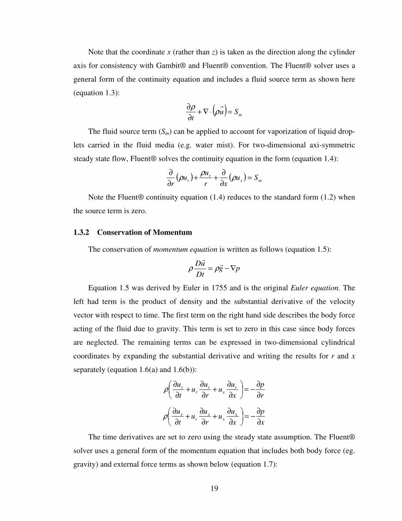
Note that the coordinate x (rather than z) is taken as the direction along the cylinder

axis for consistency with Gambit® and Fluent® convention. The Fluent® solver uses a

general form of the continuity equation and includes a fluid source term as shown here

(equation 1.3):

( ) mSut

=⋅∇+∂

∂ρ

ρ

The fluid source term (Sm) can be applied to account for vaporization of liquid drop-

lets carried in the fluid media (e.g. water mist). For two-dimensional axi-symmetric

steady state flow, Fluent® solves the continuity equation in the form (equation 1.4):

( ) ( ) mxr

r Suxr

uu

r=

∂

∂++

∂

∂ρ

ρρ

Note the Fluent® continuity equation (1.4) reduces to the standard form (1.2) when

the source term is zero.

1.3.2 Conservation of Momentum

The conservation of momentum equation is written as follows (equation 1.5):

pgDt

uD∇−=

rr

ρρ

Equation 1.5 was derived by Euler in 1755 and is the original Euler equation. The

left had term is the product of density and the substantial derivative of the velocity

vector with respect to time. The first term on the right hand side describes the body force

acting of the fluid due to gravity. This term is set to zero in this case since body forces

are neglected. The remaining terms can be expressed in two-dimensional cylindrical

coordinates by expanding the substantial derivative and writing the results for r and x

separately (equation 1.6(a) and 1.6(b)):

r

p

x

uu

r

uu

t

u rx

rr

r

∂

∂−=

∂

∂+

∂

∂+

∂

∂ρ

x

p

x

uu

r

uu

t

u xx

xr

x

∂

∂−=

∂

∂+

∂

∂+

∂

∂ρ

The time derivatives are set to zero using the steady state assumption. The Fluent®

solver uses a general form of the momentum equation that includes both body force (eg.

gravity) and external force terms as shown below (equation 1.7):

20

( ) ( ) Fpguuut

rrrrr+∇−=⋅∇+

∂

∂ρρρ

The external force vector (F) on the right hand side is included to account for fluid

interaction from dispersed phases or other user-defined sources. The body and external

forces are set to zero based on the assumed conditions for this problem.

For two-dimensional axi-symmetric steady state flow, Fluent® solves the momen-

tum equation in the following form (equation 1.8(a) and 1.8(b)):

( ) ( )r

puru

xruru

rrrxrr

∂

∂−=

∂

∂+

∂

∂ρρ

11

( ) ( )x

puru

xruru

rrxxxr

∂

∂−=

∂

∂+

∂

∂ρρ

11

The Fluent® momentum equations above can be simplified to the standard form

(equation 1.6) by neglecting external forces.

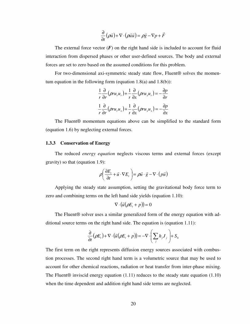
1.3.3 Conservation of Energy

The reduced energy equation neglects viscous terms and external forces (except

gravity) so that (equation 1.9):

( )upguEut

Et

trrrr

⋅∇−⋅=

∇⋅+

∂

∂ρρ

Applying the steady state assumption, setting the gravitational body force term to

zero and combining terms on the left hand side yields (equation 1.10):

( )( ) 0=+⋅∇ pEu tρr

The Fluent® solver uses a similar generalized form of the energy equation with ad-

ditional source terms on the right hand side. The equation is (equation 1.11):

( ) ( )( ) h

j

jjtt SJhpEuEt

+

⋅−∇=+⋅∇+

∂

∂∑ρρ

r

The first term on the right represents diffusion energy sources associated with combus-

tion processes. The second right hand term is a volumetric source that may be used to

account for other chemical reactions, radiation or heat transfer from inter-phase mixing.

The Fluent® inviscid energy equation (1.11) reduces to the steady state equation (1.10)

when the time dependent and addition right hand side terms are neglected.

21

1.3.4 Method of Characteristics Velocity Potential Form

The governing equations can be re-written for irrotational flow in a single second

order differential form called the velocity potential equation. The MoC calculations are

derived from the two-dimensional velocity potential equation below (Equation 1.12):

021

11

12

22

22

22

22

2=

Φ

Φ

Φ−

Φ

Φ−+

Φ

Φ−

dxdr

d

dr

d

dx

d

adr

d

dr

d

adx

d

dx

d

a

The velocity potential function (Φ) represents the full velocity potential function

where the velocity vector terms are represented by the derivatives in following equations

(Equations 1.13(a), 1.13(b) and 1.13(c)):

xudx

d=

Φ ru

dr

d=

Φ

1.3.5 Finite Volume Numerical Method Form

The governing equations can be written in a finite volume integral conservation law

form using vector notation. The integral form is implemented in the Fluent® solver

scheme and presented below (equation 1.14):

[ ] ∫∫∫ =⋅−+∂

∂VVHdVdAGFWdV

t

The vectors are given in cylindrical coordinates below (equation 1.15):

=

t

x

r

E

u

urW

ρ

ρ

ρ

ρ

( )

+

+

+=

upE

xpuu

rpuu

u

F

t

x

r

r

r

r

r

ρ

ρ

ρ

ρ

ˆ

ˆ

+

=

qu

G

jij

xi

ri

τ

τ

τ

0

The right hand term is the total enthalpy and is related to the total energy of the sys-

tem [11]. The viscous (τ) and heat flux (q) terms are set equal to zero using the

assumptions in the problem definition so that the G-vector is zero.

22

2. Methodology

The external ballistics solution process has attributes that are common between the

MoC and numerical method. The two methods use a two dimensional axi-symmetric

plane encompassing one-half of the projectile section and adjacent fluid. Both methods

use a net or mesh of points to calculate the fluid quantities of interest. However, they

take different approaches for determining these points and the parameter values at each

point.

The following sections describe the MoC and numerical method solution process

that was applied for this study. A brief discussion of the problem Reynolds number is

presented first to provide additional insight into the applicability of the Euler equation

approach.

2.1 Reynolds Number

It is convenient to characterize fluid dynamics problems using Reynolds number to

estimate the relative importance of inertial and viscous forces in the fluid system. Inertial

and viscous forces may be neglected for high Reynolds numbers (typically taken as

>107) as was assumed in the discussion of the governing equations. The Reynolds

number (Re) equation is given below for clarity (Equation 2.1):

0

00Reµ

ρvl=

Two Reynolds number calculations are completed for this problem since the characteris-

tic length (l0) may be represented by the length of small arms or artillery projectiles. A

5.56 mm small arms projectile yields a Reynolds number greater than 106, and the

Reynolds number is greater than 107 for artillery rounds comparable to the M449A1

round listed in Table 1-1. These values indicate that viscous forces are small in both

cases and support the initial assumption of inviscid flow. The values also suggest that a

turbulent flow calculation approach is warranted. However, turbulent flow and associ-

ated field features are neglected in both calculation methods to reduce solution

complexity.

23

2.2 Method of Characteristics

The MoC is based on the velocity potential analytic method that reduces the govern-

ing second order differential equations to a first order form that have exact solutions

along specific curves called characteristic lines. Flow parameters such as velocity or

pressure are quantified at the intersections of these lines using compatibility equations,

the characteristic lines and the problem boundary conditions. The MoC has been applied

to compressible flow problems since the late 1920’s, and several different implementa-

tion approaches have been utilized [1] [12] [13] [14] [15]. Though the solutions are

mathematically exact, the implementation process introduces potential inaccuracies. The

following discussion outlines the process and equations used herein.

2.2.1 Process

The MoC calculations begin with a definition of the physical plane consisting of the

projectile and surrounding fluid volume. The physical plane is presented in Figure 2-1.

Figure 2-1: Method of Characteristics Physical Plane

24

The fluid volume is defined in terms of the projectile base diameter and employs to

reduce its scale. The axi-symmetric volume starts 5 diameters ahead of the projectile

nose, ends 30 diameters downstream of its base, and extends 20 diameters away from the

center axis. The region size was determined through examination of other research to

capture the entire shock or expansion flow disturbances near the projectile [3] [4] [6].

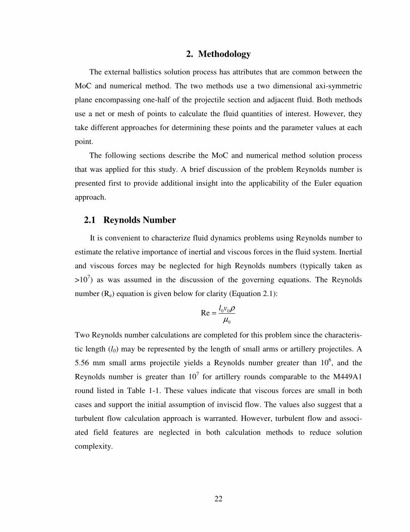
Once the physical plane is established, a calculation is performed to determine the

location of the shock front. The shock front is defined by the set of positive characteris-

tic line intersection points. The positive characteristic lines are determined for a set of

points parallel to and near the projectile axis in the inflow region upwind (to the left) of

the projectile, and lie on the projectile surface. The set of points and spacing is chosen to

ensure the fluid volume contains sufficient intersection points with negative characteris-

tic lines in later calculations. A partial set of positive characteristic lines and the

intersection points defining the shock front are shown in Figure 2-2.

Figure 2-2: Location of the Shock Front

25

The figure shows red circles at the positive characteristic line intersection points,

and indicates that the shock front can be represented as a straight line extending from the

projectile tip coordinates at a slope defined by the inflow boundary condition. Adjacent

characteristic lines diverge adjacent to the ogive section immediately downstream of the

shock front. This feature represents fluid expansion. The characteristic lines return to a

parallel condition where the ogive merges into the body section.

The characteristic line slope, r-intercept and a Mach number are calculated at the

point coordinates using the inflow boundary condition, turn angle (θ), characteristic line

slope and compatibility equations. The characteristic line slope and compatibility

equations are obtained from the governing equation presented in section 1.3.4, and

summarized in sections 2.2.2.1 and 2.2.2.2.

The shock front divides the physical plane into an inflow region (region 1) and a

downstream region behind the shock (region 2). The last positive characteristic line

located at the base of the projectile is a Mach line that defines the forward portion of the

base Mach line. This line is taken as a convenient surface to terminate the volume of

interest. Flow downstream of the base (region 3) is not evaluated with the MoC. The

three regions are annotated in Figure 2-3.

Shock and Expansion Fan Overview

Shock FrontMach Line

Expansion Fan

Forward Mach Line

θfan = 30.03°

θshock = 30.00°

Note: Accurate estimates could not be obtained from oblique shock relations due to shape complexity

1 2 3

Figure 2-3: Partition of the Physical Plane

26

The Mach lines in Figure 2-3 separate each region and extend to the limits of the

physical plane. The horizontal dotted line is shown for angle reference. The fluid field

Mach number and turn angles are calculated separately for regions 1 and 2. The calcula-

tions start in a manner similar to the calculations that were performed to locate the shock

front. Supporting equations are presented in Section 2.2.2.

For region 1 upwind of the projectile, positive and negative characteristic lines are

plotted using the equation in section 2.2.2.1 and the arbitrary set of points along the axis

and inflow boundaries. The lines are extended through region 1 up o the shock front

location. Intersections between positive and negative characteristic lines are determined

to form a characteristic net of points in the region. The flow field Mach number and turn

angle conditions are transferred to each point using the compatibility equations in

section 2.2.2.2. The corresponding pressure value is obtained from the Mach number

using the isentropic flow relation in section 2.2.2.5. Though initiated from the axis and

inflow boundary in this case, the calculations can be started from any of the region 1

boundaries with the same end result. Note the process described above yields a homoge-

neous field speed and turn angle so the characteristic net point density can be low to

reduction calculation time.

The calculations for region 2 are similar to the process for region 1 with one signifi-

cant modification relating to the negative characteristic lines. Two processes are applied

to generate these lines. The first process utilizes the points on the projectile surface to

project negative characteristic lines to the forward shock front Mach line. These lines

provide intersections with positive characteristic lines near the projectile, but do not

define intersections at larger radial distances or towards the projectile base. Therefore, a

second process is employed to create negative characteristic lines through the positive

characteristic line intersection points that defined the shock front at further distances

from the projectile. The second procedure is outlined in section 2.2.2.3 and determines a

local Mach angle (β) from the turn and Prandtl-Meyer angles for the intersecting positive

characteristic lines. This procedure can be applied to the entire region achieving nearly

the same result as the two step process. However, the two step process was chosen

because it did not rely on iterative calculations for the fluid closest to the projectile. The

resulting characteristic net and intersection points are illustrated in Figure 2-4.

27

Figure 2-4: Characteristic Net and Intersection Points

The figure shows positive characteristic lines (dark blue), negative characteristic

lines (green), the inflow region intersection points (black circles), the shock front points

(fuscia), and the downstream intersection points (red). The projectile is outlined in black.

Note the intersection point density is highest near the projectile nose where higher

gradients are anticipated, and lower throughout the inflow region (region 1) where the

fluid parameters are constant. The flow field Mach number and turn angle conditions are

transferred to each point in region 2 just as it was done for region 1 using the compatibil-

ity equations in section 2.2.2.2. The corresponding pressure value is obtained from the

Mach number using the isentropic flow relation in section 2.2.2.5. The region 2 calcula-

tions rely on the conditions at the shock front or projectile surface so results cannot be

obtained if the calculations are initiated from the upper inflow/outflow boundary condi-

tion.

28

2.2.2 Equations

The following sections present equations that are used to develop the characteristic

net and determine Mach number, turn angle and static pressure at the net points. The

equations are derived from isentropic flow, normal and oblique shock relations, and are

readily obtained from a variety of textbooks. Brief descriptions of the most relevant

equations are provided for clarity.

2.2.2.1 Characteristic Line Slope

The characteristic lines for two dimensional axi-symmetric irrotational flow prob-

lems are represented by the integral solutions to the following linear differential equation

(Equation 2.1):

( )µθ ±=

tan

chardx

dr

Equation 2.1 divides the characteristic lines into two subsets labeled C+ when (θ+µ)

is used and C– for the (θ–µ) term. Both sets of characteristic lines are straight Mach

lines for the external ballistic problem though this may not be the case for other classes

of problems.

2.2.2.2 Compatibility

The compatibility equations are also derived from the governing equations for two

dimensional axi-symmetric irrotational flow problems and represented by the integral

solutions to the following linear differential equations (Equation 2.2(a) and 2.2(b)):

(along C– characteristics) ( )

−−=+

r

dr

Md

θυθ

cot1

1

2

(along C+ characteristics) ( )

+−=−

r

dr

Md

θυθ

cot1

1

2

Note the values (θ+ν) and (θ–ν) are dependent on the radial coordinate of the point

and are undefined (infinite) for zero turn angle (θ) and radius distance (r). A small angle

of attack (α=0.0014 degrees) is added to the turn angle throughout the flow field, and a

small radius offset (r=0.00001 base diameters) is applied to the points in the inflow

region ahead of the projectile to ensure finite results throughout the calculations. The

29

differential terms on the left hand side are replaced by finite differences to solve equa-

tion 2.2 at each intersection point.

2.2.2.3 Local Mach Angle Calculation

The iterative procedure for calculating the negative characteristic line slope at the

shock front starts with the θ–β–M relation (Equation 2.3):

( )( )

++

−=

22cos

1sincot2arctan,

2

22

βγ

βββθ

M

MM

An initial β is assumed for the first iteration. Here γ is an assumed constant for air

and the upstream Mach is used. The resulting turn angle is used to calculate a Mach

number immediately downstream of the shock through the normal component of the

inflow velocity and normal shock relations [1]. Once the downstream Mach number is

known, the Prandtl-Meyer angle can be determined and a positive characteristic line

compatibility value (θ–ν) is calculated. The process is repeated until a local Mach angle

is found that produces the desired positive characteristic line compatibility value within

some acceptable tolerance value . A table consisting of local Mach angle, turn angle,

downstream Mach number, Prandtl-Meyer angle and positive characteristic line com-

patibility values was interpolated (look up the desired value for θ–ν) to eliminate the

iterative process.

2.2.2.4 Prandtl-Meyer Function

The compatibility equations include a Prandtl-Meyer angle term that is obtained

from the Prandtl-Meyer function. The value of this function is given by (Equation 2.4):

( ) ( ) ( )1arctan11

1arctan

1

1 22 −−−−

+

−

+= MMM

γ

γ

γ

γυ

It is possible to obtain a value for this angle at points in the physical plane where

characteristic lines intersect. The corresponding Mach number is determined by iterative

application of equation 2.4 or other more efficient techniques. A table of ν vs. Mach

number was interpolated to eliminate the iterative process.

30

2.2.2.5 Pressure

The ratio of static pressure (p) to total or stagnation pressure (p0) is related to the

local Mach number at a point in the physical plan by the isentropic flow relationship

(Equation 2.5):

120

2

11

−

−+=

γ

γ

γM

p

p

Note the definition of total pressure is derived using the isentropic flow assumption

and has limited applicability to the supersonic external ballistics problem because the

flow field may not be considered isentropic in many cases.

2.3 Numerical Method

The finite volume numerical method is a shock capturing mathematic approach that

estimates the solution to the governing differential equations using boundary conditions

given in the problem definition [1]. The boundary conditions typically include geometric

(e.g. projectile wall) and fluid property (e.g. constant inflow velocity) constraints, and do

not require prior knowledge of major flow gradients. The obvious advantage is that flow

features may be predicted or captured by analysis without thorough experimentation or

prior experience with similar flow problems. The solution method is not mathematically

exact and like the MoC may not capture all of the expected flow field physics.

The numerical method calculations apply an implicit second order upwind finite

volume calculation through Fluent® software to solve the inviscid Euler equations in

integral form described in section 1.3 [11]. Fluent® has been structured to solve the

governing equations in either a pressure or density based form.

31

A control volume calculation technique is utilized regardless of the solver choice.

The general procedure steps are outlined below.

• The physical plane is divided into discrete control volumes using a mesh or grid

• The integral equations are solved for each control volume to yield algebraic linear

equations for dependent variables such as velocity, pressure and other conserved

scalar parameters

• The system of algebraic linear equations is solved to yield updated values of the

dependent variables

Further details regarding the pressure and density based solvers and more specific

calculation procedures are provided in section 2.3.2.1.

2.3.1 Mesh Generation

The physical plane mesh is generated in Gambit® software using an x-y plane that

extends outward from the projectile axis where distance is measured in projectile base

diameters [16]. The y-direction is translated into an axi-symmetric r-direction once the

mesh and boundary conditions are imported into Fluent® and the axi-symmetric solver

feature is selected.

The mesh is 20 diameters radial by 40 diameters axial and is positioned forward of

the projectile nose by 5 diameters (or 1 projectile length) for consistency with the MoC

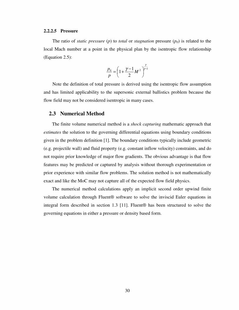
calculations. The resulting physical plane is annotated with boundary labels and shown

in Figure 2-5. The figure content is identical to MoC Figure 2-1.

32

Physical Plane Illustration

Inflow Boundary

Wall Boundary

Outflow Boundary

Upper Inflow / Outflow Boundary

Flow

Figure 2-5: Physical Plane Mesh

A structured grid requires less memory, provides superior accuracy and allows a

better boundary-layer resolution than an unstructured grid for most solvers. A structured

grid also provides a better resolution around sharp leading and trailing edges by having

cells with a large aspect ratio in these regions. Then numerical calculations herein use

the structured grid.

A mesh density study is performed to evaluate solution accuracy as a function of

nodal spacing. Three mesh sizes were selected based on their scale compared to the

projectile base radius (the smallest dimension on the physical plane) and with considera-

tion towards scales that were applied by other researchers conducting more complex

turbulence research. The three mesh sizes are labeled coarse, medium and fine where the

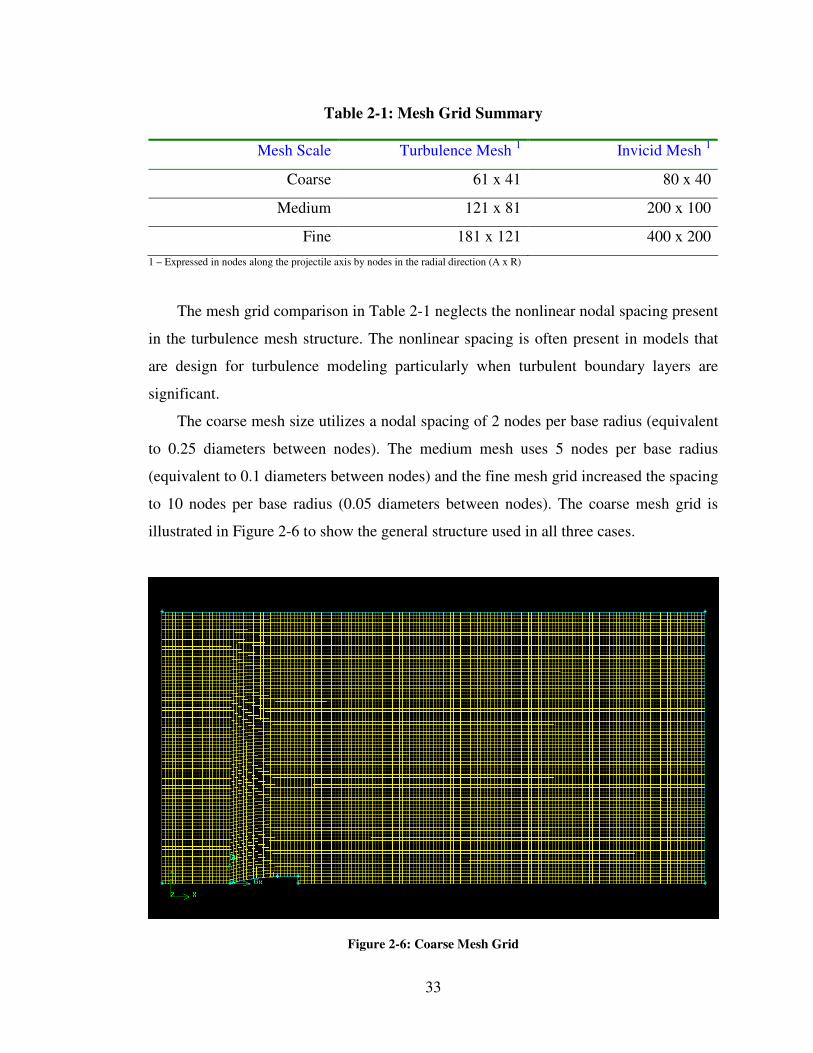
mesh densities are comparable to referenced research literature [3]. The comparison is

presented in Table 2-1.

33

Table 2-1: Mesh Grid Summary

Mesh Scale Turbulence Mesh 1 Invicid Mesh

1

Coarse 61 x 41 80 x 40

Medium 121 x 81 200 x 100

Fine 181 x 121 400 x 200

1 – Expressed in nodes along the projectile axis by nodes in the radial direction (A x R)

The mesh grid comparison in Table 2-1 neglects the nonlinear nodal spacing present

in the turbulence mesh structure. The nonlinear spacing is often present in models that

are design for turbulence modeling particularly when turbulent boundary layers are

significant.

The coarse mesh size utilizes a nodal spacing of 2 nodes per base radius (equivalent

to 0.25 diameters between nodes). The medium mesh uses 5 nodes per base radius

(equivalent to 0.1 diameters between nodes) and the fine mesh grid increased the spacing

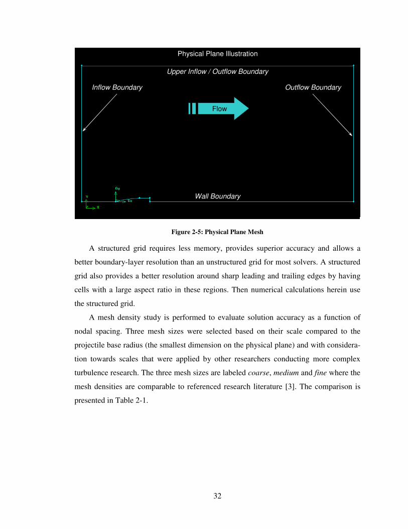
to 10 nodes per base radius (0.05 diameters between nodes). The coarse mesh grid is

illustrated in Figure 2-6 to show the general structure used in all three cases.

Figure 2-6: Coarse Mesh Grid

34

The physical plane, mesh grids and boundary conditions were created in a Fluent®

compatible file format (*.msh) using Gambit® software. Gambit® uses primitive shapes

(points, lines, polygons and ellipses) and Boolean operations (and, or, xor, etc.) to create

objects in physical space that can be used to create a mesh grid, boundaries and an

interior fluid. The general steps of this process are outlined below.

• Create a new Gambit® model file

• Generate the object using primitive shapes and Boolean operations

• Generate a fluid boundary around the object

• Merge the object and fluid boundary to create a physical plane

• Generate a mesh grid from the physical plane (check mesh utilities are available)

• Define the object and fluid boundaries by type (valid types are pre-defined)

• Define an interior fluid (optional since this can also be done in Fluent®)

• Save the Gambit® model file

• Export the mesh grid, boundaries and interior fluid (use the *.msh format)

The Gambit® software is capable of 3-dimensional object structures and offers an

extensive range of import and export file formats though these capabilities were not

utilized in the course of this study.

2.3.2 Fluent® Implementation

The general steps of the numerical solution process were taken from Fluent® Tuto-

rial 3 and are outlined below. Fluent® Version 6.2 software was used.

• Read the mesh grid file (*.msh) exported from the Gambit® software application

• Perform a grid check and reorder the domain to reduce computation time

• Choose a solver

• Define fluid and viscosity models

• Apply the boundary conditions

• Set the solver parameters (courant number, relaxation & under-relaxation factors)

• Set the solver accuracy (1st order, 2

nd order, etc.)

35

• Set the residual error monitors and convergence limits (implicit solver only)

• Initialize the solution

• Iterate the solution until satisfactory convergence is achieved

Each of these steps involves little effort to implement though some of the choices

have substantial impact on the type of solution obtained, rate of solution convergence

and accuracy. The more involved steps are shown in italics and discussed in further

detail below.

2.3.2.1 Solver Selection

Choose a solver – A pressure-based and density-based solver is available for the

calculation. The pressure-based approach was originally developed for low-speed

incompressible flows while the density-based approach was mainly used for high-speed

compressible flows. The current software release contains updates that reformulate and

extend each method to solve for a wide range of flow conditions beyond their original

intent. Both methods apply the same technique to obtain the velocity field from the

momentum equations. However, there are differences with regard to the pressure solu-

tions. In the density-based approach, the continuity equation is used to obtain the density

field while the pressure field is determined from the equation of state. The pressure-

based approach obtains the pressure field using a specific algorithm that belongs to a

general class of methods called the projection method. In the projection method, the

mass conservation (continuity) constraint of the velocity field is achieved by solving a

pressure (or pressure correction) equation. The pressure equation is derived from the

continuity and the momentum equations in such a way that the velocity field, corrected

by the pressure, satisfies continuity. Since the governing equations are nonlinear and

coupled, the solution process involves iterations where the entire set of governing

equations is solved repeatedly until the solution converges.

Though both solvers were evaluated, the results for the density-based solver are pre-

sented herein since this solver converged faster than the pressure-based solver. The

density based solver was also considered appropriate because it was originally designed

for incompressible supersonic flow problems. An implicit formulation with the Green-

36

Gauss Cell Based gradient option was selected arbitrarily. The remaining options were

easily determined from the problem definition. The 2D option is selected to indicate that

the problem is two-dimensional. The axi-symmetric option is used since solution domain

is in cylindrical coordinates rather than a Cartesian coordinate system, and a steady state

solution is desired so the steady state feature is chosen.

2.3.2.2 Boundary Condition Implementation

Apply the boundary conditions – Several boundary condition categories are pro-

vided for defining problem geometry. Two types were selected for this problem as

described in further detail below.

The inflow, outflow and upper inflow/outflow boundary conditions are implemented

with a pressure far field condition used for virtual (or cut) fluid boundaries where the

inflow or outflow characteristics are not necessarily known. This boundary type accepts

an initial speed, direction vector and reference pressure input. The problem definition in

section 1.2 indicates initial conditions are Mach 2.0 with zero degrees angle of attack (α)

at standard atmospheric pressure (101325 Pa) and temperature (300K). Fluid flow is

permitted in any x-r plane direction during the implicit calculation process.

The axis (or centerline) and projectile wall boundary is set using a wall condition

that enforces parallel flow (or zero normal flow) along the surface. Other boundary types

including the axis and symmetry boundary were considered, but determined to be inap-

propriate for this boundary case because they generated software execution warnings. It

is noted that special attention must be applied when employing numerical solution

methods to the sharp corner wall condition at the outer radius of the projectile base. The

values for pressure, density and temperature at the corner should utilize conditions at the

projectile wall rather than at the center axis, and values at the intersection of the center

axis and base should use conditions along the center axis rather than the projectile wall.

2.3.2.3 Solver Control

Set the solver parameters – The density based solver employs options for discretiza-

tion, Courant number and flux type. The discretization option establishes the numerical

method for the calculations. In this case, a second order upwind method is applied. The

37

Courant number controls the time step size, solution stability and rate of convergence.

Values between 5 and 20 were applied for this calculation. The flux type option de-

scribes the flux splitting scheme that is employed in the calculation. The Roe Flux-

Difference Splitting (Roe-FDS) was applied to this problem because the alternative

(Advection Upstream Splitting Method or AUSM) scheme did not yield a converging

solution.

2.3.2.4 Solution Monitoring and Convergence

Set the residual error monitors and convergence limits – Implicit method solvers

use differences between physical parameters such as fluid continuity (conservation of

mass), velocity or energy from one iteration step to the next step as a means of determin-

ing when a level of solution accuracy is achieved. This difference is called residual error

and is generally considered favorable as the value approaches zero. Error values that

oscillate without approaching zero are considered unsatisfactory. Fluent® offers stan-

dard residual error monitors that calculate and compare continuity, velocity and total

energy values averaged over the entire mesh grid. The software also offers user-specified

residual error monitors with a variety of capabilities. For this evaluation, standard

residual error monitors were set for continuity (conservation of mass), x-velocity, y-

velocity and total energy. The solution was considered to have converged when the

continuity residual error values were less than 1 x 10-5

kg, x-velocity and r-velocity was

less than 0.001 m/s, and total energy was less than 1 x 10-6

joules. A user specified

convergence monitor was created for the projectile drag coefficient so the result could be

compared to empirical data [2]. The drag coefficient (Cd) was considered satisfactory

provided a constant value with no oscillation was noted towards the end of the solution.

In practice, the density based numerical solution met the residual error and conver-

gence criteria with no application warnings or divergence detection. The pressure based

solver did not yield a satisfactory result when initialized with a supersonic boundary

condition. However, a converged solution was obtained by incrementally increasing the

boundary velocity from a subsonic condition to the desired supersonic condition. In

other words, the solution at the desired flow condition was achieved with few warnings

and no errors by dividing the problem into a series of lower velocity problems where the

38

results from the previous velocity condition provided an initial solution for the next

(higher) velocity condition. The initial boundary condition was set to a velocity of Mach

0.8 and iterated until the residual errors were less than the previously specified limits,

and the drag coefficient had converged to a single non-oscillating value. Next, the

velocity boundary condition was increased to Mach 1.5, 1.75 and finally the desired

condition, Mach 2.0. The aforementioned residual error and convergence criteria were

not achieved for the intermediate velocity conditions (Mach 1.5 and 1.75) though the

solver relaxation parameter was reduced slightly (from 0.75 to 0.70) to prevent the

occurrence of an oscillating drag coefficient value. A similar approach was tested to

rapidly obtain a solution for the axi-symmetric option using 2-dimensional Cartesian

coordinate results. In each case, the final pressure based solutions were similar to the

density based solutions when the same convergence criteria were met. The density based

solver proved capable of achieving smaller convergence criteria compared to the pres-

sure based solver.

The technique of applying the results from one solution to initialize another solution

proved useful as a means of overcoming specific problems encountered during both

medium and fine mesh grid solutions, and may in fact be beneficial when solving other

problem types. These lessons were considered sufficiently valuable to retain here even

though the pressure based solver results are not utilized.

The models and solutions are stored in Fluent® case files for use with the Fluent®

software. The solutions are exported in comma separated value ASCII format and read

into Matlab® and Microsoft Excel® for comparison to the MoC results.

39

3. Results and Discussion

A critical view of any analysis is an important step to determining its accuracies and

limitations, and can be achieved through comparison to other analytic, numerical or

experimental works. In this study, the comparison between two calculation methods is

the primary focus. Additional quantitative and qualitative comparisons are performed

using experimental data and like research where possible. The following sections discuss

the comparisons between MoC and numerical solutions with concentration of the

representation of the velocity field. Selected results for the pressure field and calculation

of projectile drag coefficient are also examined and compared to results from other

sources. One such source is an experimental result for a similar supersonic projectile that

illustrates the anticipated shock front and flow expansion characteristics. Other field

parameters such as entropy or enthalpy have not been interrogated in any detail and the

corresponding physics may not be adequately represented by any of the solutions

presented herein. The following sections present the experimental illustration and

comparisons between MoC and numerical solution results for the coarse, medium and

fine mesh models.

3.1 Experimental Illustration

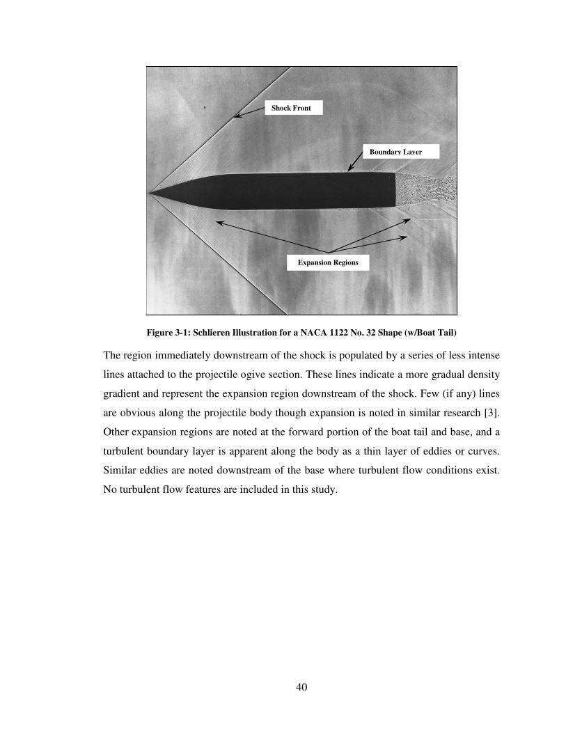
An experimental result for a NACA No. 32 projectile travelling at Mach 1.5 is

shown in Figure 3-1 and illustrates the anticipated near-field fluid shock and expansion

wave characteristics. The figure contains a Schlieren (or shadowgraph) photograph of

the projectile travelling from right-to-left (right is downstream). The dark lines in the

fluid represent high density gradients that distort the column of light entering the cam-

era. A straight dark line extends from the projectile nose at an angle to the projectile

axis. This density gradient is caused by the shock front where the angle corresponds to

the inflow speed condition. Vorticity is not apparent in the flow since the shock front

appears straight throughout the image. Though theory does not readily define a thickness

to the shock front gradient, it is generally taken to have a thickness equal to the mean

free path between air molecules at the specified environmental condition. For air near

the Earth’s surface, this value is on the order of 10-6

meters and can therefore be ne-

glected for practical projectile sizes.

40

Figure 3-1: Schlieren Illustration for a NACA 1122 No. 32 Shape (w/Boat Tail)

The region immediately downstream of the shock is populated by a series of less intense

lines attached to the projectile ogive section. These lines indicate a more gradual density

gradient and represent the expansion region downstream of the shock. Few (if any) lines

are obvious along the projectile body though expansion is noted in similar research [3].

Other expansion regions are noted at the forward portion of the boat tail and base, and a

turbulent boundary layer is apparent along the body as a thin layer of eddies or curves.

Similar eddies are noted downstream of the base where turbulent flow conditions exist.

No turbulent flow features are included in this study.

Shock Front

Expansion Regions

Boundary Layer

41

3.2 Quantitative Comparisons

The MoC results are not easily compared to the numerical solutions due to the addi-

tional assumptions of isentropic irrotational flow, and because the characteristic net

consists of irregularly spaced points. However, quantitative comparisons are possible for

a subset of the MoC results including:

• Angle of the shock front relative to the projectile axis

• Shock front attachment to the projectile

• Angle of the Mach line at the projectile base

• Mach number immediately downstream of the shock front

• Minimum Mach number magnitude and position near the projectile

• Mach number and pressure along the projectile surface

Each of these topics is discussed in the following paragraphs. It is recognized that

surface or point-for-point field comparisons are possible using an interpolation routine or

iterative refinements to characteristic net. However, development of an interpolation

routine or data tabulation was not considered to add substantially to new understanding

of the problem.

Angle of the shock front relative to the projectile axis – The MoC calculation pro-

duces a shock front at an angle of 30 degrees with respect to the projectile axis. The

angle is set by the inflow boundary condition Mach number. The shape of the shock

front is addressed later in section 3.3.

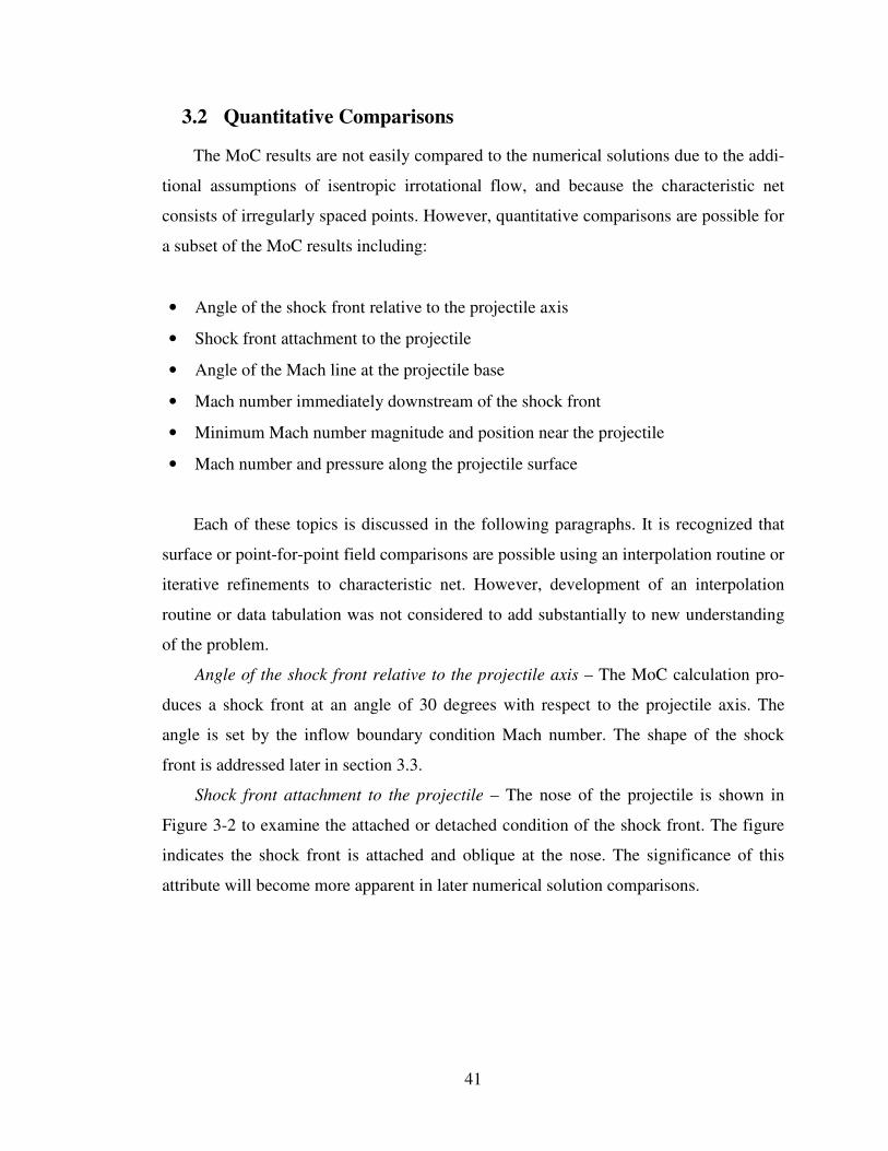
Shock front attachment to the projectile – The nose of the projectile is shown in

Figure 3-2 to examine the attached or detached condition of the shock front. The figure

indicates the shock front is attached and oblique at the nose. The significance of this

attribute will become more apparent in later numerical solution comparisons.

42

Figure 3-2: Verification of Shock Attachment

Angle of the Mach line at the projectile base – As noted earlier, the positive charac-

teristic lines in the ogive section diverge as radial distance increases. The characteristic

lines return to a parallel orientation at the transition to the body section and form an

angle to the projectile axis that is nearly equal to the inflow region. The Mach line at the

base of the projectile is oriented at 30.03 degrees relative to the projectile axis and

represents the base region expansion fan forward Mach line. The label is selected to

recognize that the positive characteristic lines form a fan similar to the lines intersecting

the ogive and denote an expansion region downstream of the base. The characteristic

line fan terminates when flow detaches from the base of the projectile.

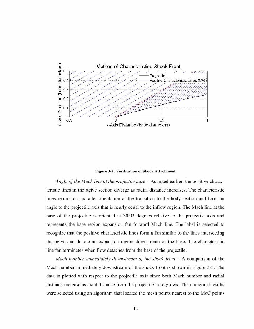
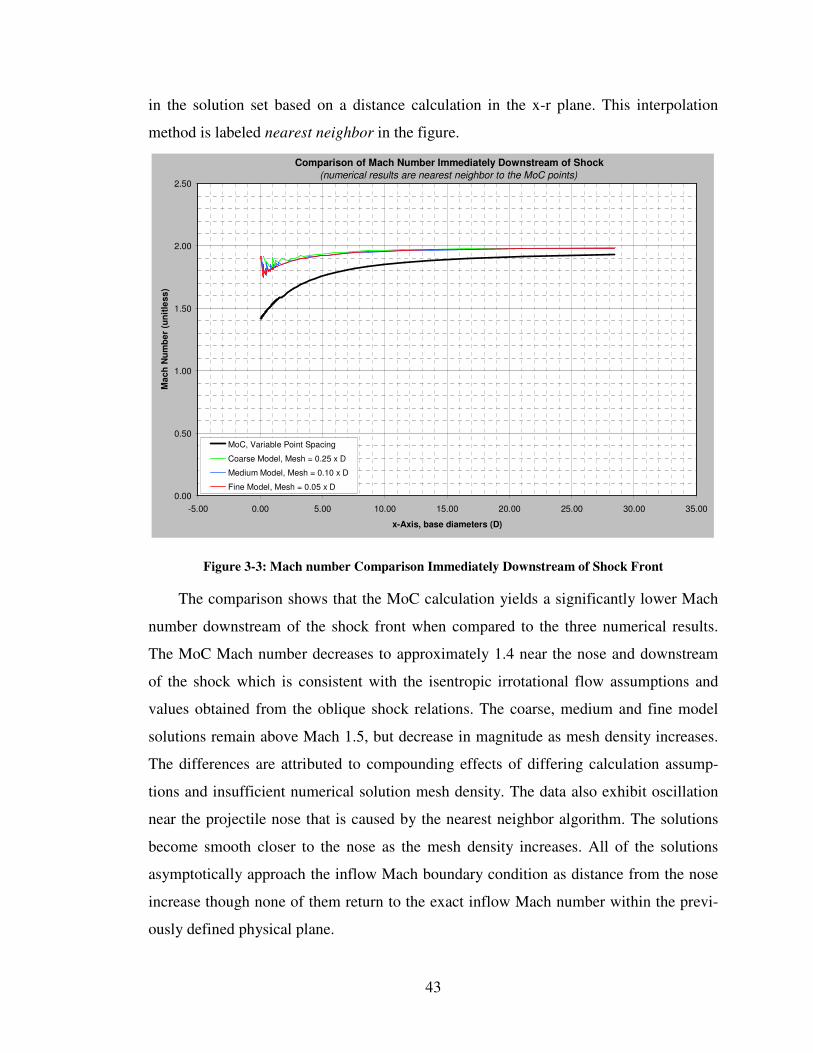
Mach number immediately downstream of the shock front – A comparison of the

Mach number immediately downstream of the shock front is shown in Figure 3-3. The

data is plotted with respect to the projectile axis since both Mach number and radial

distance increase as axial distance from the projectile nose grows. The numerical results

were selected using an algorithm that located the mesh points nearest to the MoC points

43

in the solution set based on a distance calculation in the x-r plane. This interpolation

method is labeled nearest neighbor in the figure.

Comparison of Mach Number Immediately Downstream of Shock

(numerical results are nearest neighbor to the MoC points)

0.00

0.50

1.00

1.50

2.00

2.50

-5.00 0.00 5.00 10.00 15.00 20.00 25.00 30.00 35.00

x-Axis, base diameters (D)

Ma

ch

Nu

mb

er

(un

itle

ss

)

MoC, Variable Point Spacing

Coarse Model, Mesh = 0.25 x D

Medium Model, Mesh = 0.10 x D

Fine Model, Mesh = 0.05 x D

Figure 3-3: Mach number Comparison Immediately Downstream of Shock Front

The comparison shows that the MoC calculation yields a significantly lower Mach

number downstream of the shock front when compared to the three numerical results.

The MoC Mach number decreases to approximately 1.4 near the nose and downstream

of the shock which is consistent with the isentropic irrotational flow assumptions and

values obtained from the oblique shock relations. The coarse, medium and fine model

solutions remain above Mach 1.5, but decrease in magnitude as mesh density increases.

The differences are attributed to compounding effects of differing calculation assump-

tions and insufficient numerical solution mesh density. The data also exhibit oscillation

near the projectile nose that is caused by the nearest neighbor algorithm. The solutions

become smooth closer to the nose as the mesh density increases. All of the solutions

asymptotically approach the inflow Mach boundary condition as distance from the nose

increase though none of them return to the exact inflow Mach number within the previ-

ously defined physical plane.

44

Minimum Mach number magnitude and position near the projectile – The MoC,

coarse, medium and fine model solutions were evaluated to locate the minimum Mach

number and position in the physical plane. The results are presented in Table 3-1.

Table 3-1: Minimum Mach number Comparison

Source

Position

x-Axis

Position

r-Axis

Distance

to Nose

Local

Mach

Method of Characteristics 0.0312 0.0180 0.0360 1.4282

Coarse Mesh Model 0.9834 0.2441 1.0132 1.7960

Medium Mesh Model 0.4892 0.1320 0.5067 1.7338

Fine Mesh Model 0.2405 0.0675 0.2498 1.7124

The table shows the MoC minimum Mach number is lower and located closer to the

projectile nose than all three numerical model results. As noted in discussion of Figure

3-3, the MoC values assume isentropic irrotational flow to obtain a solution. The nu-

merical solution trend also suggest that the local Mach will converge towards the MoC

value with increasing mesh density though it is not clear that the MoC value will be

achieved.

Mach number and pressure along the projectile surface – The MoC, coarse, me-

dium and fine model solutions for Mach number along the projectile surface are

presented in Figure 3-4. The MoC Mach number decreases sharply from the inflow

Mach number to the minimum Mach value almost immediately at the projectile nose.

The values increase linearly throughout the ogive section and are equal to the inflow

Mach number downstream of the intersection between the ogive and body sections at

3.50 base diameters from the nose. The sharp decrease at the projectile nose indicates a

sharp gradient or discontinuity in the flow field corresponding to the formation of the

shock front. The steadily increasing Mach number over the ogive section corresponds to

flow expansion. Both the magnitude and trend shown here are similar to earlier MoC

calculations performed for a missile ogive at Mach 2 [13]. The observation that the

Mach number remains constant and equal to the inflow Mach number across the body

section suggests that no shock or expansion occurs in the adjacent fluid region. The

45

coarse, medium and fine model solutions are less than the inflow Mach number at the

projectile nose and decrease gradually over the first base diameter distance of the ogive

section. The coarse model result achieves its minimum value at a distance of approxi-

mately 0.983 base diameters. The medium and fine model results achieve their minimum

values at 0.489 and 0.241 base diameters respectively. The fine model results exhibit the

sharpest gradient at the projectile nose.

Projectile Surface Mach Number

0.00

0.50

1.00

1.50

2.00

2.50

0.00 0.50 1.00 1.50 2.00 2.50 3.00 3.50 4.00 4.50 5.00


Ma

ch

Nu

mb

er

(un

itle

ss

)





Figure 3-4: Projectile Surface Mach number Comparison

The numerical solutions increase linearly downstream of their respective minimum

values, and continue to increase through the transition between the ogive and body

sections. All three solutions nearly return to the inflow Mach number at the projectile

base. The trend in the coarse, medium and fine model results indicate that the position of

the minimum Mach number at the projectile surface is converging towards the MoC

minimum value. The solution trend at the intersection point between the ogive and body

sections of the projectile indicate that the fluid undergoes weak expansion just down-

stream of this point. The existence of this expansion region is not easily identifiable in

the experimental illustration, but has been reported in other research [3].

Mach Gradient

Weak Expansion

46

The projectile surface pressures corresponding to Figure 3-4 are not readily com-

pared because the MoC calculations generate a pressure ratio while the numerical

solutions provide absolute flow field pressures. Therefore, the pressure results are

presented separately in Figure 3-5 and Figure 3-6.

Method of Characteristics

0.10

0.15

0.20

0.25

0.30

0.0 0.5 1.0 1.5 2.0 2.5 3.0 3.5 4.0 4.5 5.0


Sta

tic t

o T

ota

l P

ressu

re R

ati

o, p

/ p

0 (

un

itle

ss)

Reference Value


Figure 3-5: Method of Characteristics Projectile Surface Pressure Ratio

Figure 3-5 presents the MoC static to total (or stagnation) pressure ratio from the

nose to the base of the projectile. The value far ahead of the projectile is provided as a

reference value. The data shows that the pressure ratio changes sharply achieving a

maximum value near 0.3 at the projectile nose and decreases to the far field value

(~0.128) at the transition between ogive and projectile body sections. The values never

drop below the far-field ratio adjacent to the projectile. Conclusions cannot drawn from

the pressure ratio because the total pressure is not constant throughout the flow field.

Note the green circles shown in the figure denote the MoC calculation points.

47

Numerical Solution Comparison

0.8

0.9

1.0

1.1

1.2

1.3

1.4

1.5

0.0 0.5 1.0 1.5 2.0 2.5 3.0 3.5 4.0 4.5 5.0


Sta

tic P

ress

ure

Rati

o, p

/ p

∞∞ ∞∞ (

un

itle

ss

)

Reference Value




Figure 3-6: Numerical Model Pressure Ratio

Figure 3-6 presents the static pressure values along the projectile surface referenced

to the static pressure far ahead of the projectile. Again the far field value is provided as a

reference. Like the previous Mach number comparisons, the pressure ratio increases

immediately downstream of the nose indicating a shock front. The sharpness of the

gradient varies with mesh density where the fine model exhibits the highest slope. The

pressure ratios then decrease to a minimum value near the intersection of the ogive and

body sections at ~3.5 diameters. The minimum value is below the far field reference

indicating further expansion downstream of the ogive. Experimental data and numerical

results presented by Cummings (see Figure 12 of the referenced paper) show that such

an expansion occurs for similar shape projectiles at a higher Mach number and zero

angle of attack [3]. Cummings’ numerical results and experimental data indicate the

pressure ratio transitions unity sharply near the ogive-body intersection whereas the data

presented above shows no change in gradient as the pressure transitions unity ahead of

the intersection between the ogive and body section. The comparison to other research

does not yield a clear conclusion due to differences in calculation methods.

48

3.3 Qualitative Comparisons

Qualitative comparisons are completed for selected MoC solution attributes and the

coarse, medium and fine model results. The selected MoC attributes are the shock front

and base expansion fan forward Mach lines. These lines are overlaid on each numerical

solution to facilitate comparisons. Both contour and surface graphical formats are

provided to assist in data interpretation. The comparisons are presented in the following

sections and restricted to Mach number and static pressure fields.

3.3.1 Coarse Mesh

The coarse mesh Mach field is presented in Figure 3-7 and Figure 3-8 for the entire

physical plane. Figure 3-7 depicts Mach number contour lines, and Figure 3-8 shows the

same data in a filled contour surface plot format. The contour lines in Figure 3-7 show a

gradient that runs at an angle similar to the MoC shock front Mach line. However, the

gradient contours are not straight lines. Close examination of the gradients at the nose

suggest that the shock is detached from the projectile and normal to the inflow velocity

vector. The Mach number immediately behind the apparent shock front decreases in

amplitude to approximately 1.8 and appears to return to the inflow condition near the

projectile base. The Mach number increases steadily throughout region 2 adjacent to the

ogive section and continue to increase adjacent to the body section indicating fluid

expansion. The Mach number has nearly returned to the inflow Mach number at the base

Mach line. The contours also appear normal to the projectile surface parallel flow or slip

at the wall. The presence of a thick wake is apparent and detaches from the projectile

base. The thick wake is not apparent in the experimental illustration from section 3.1.

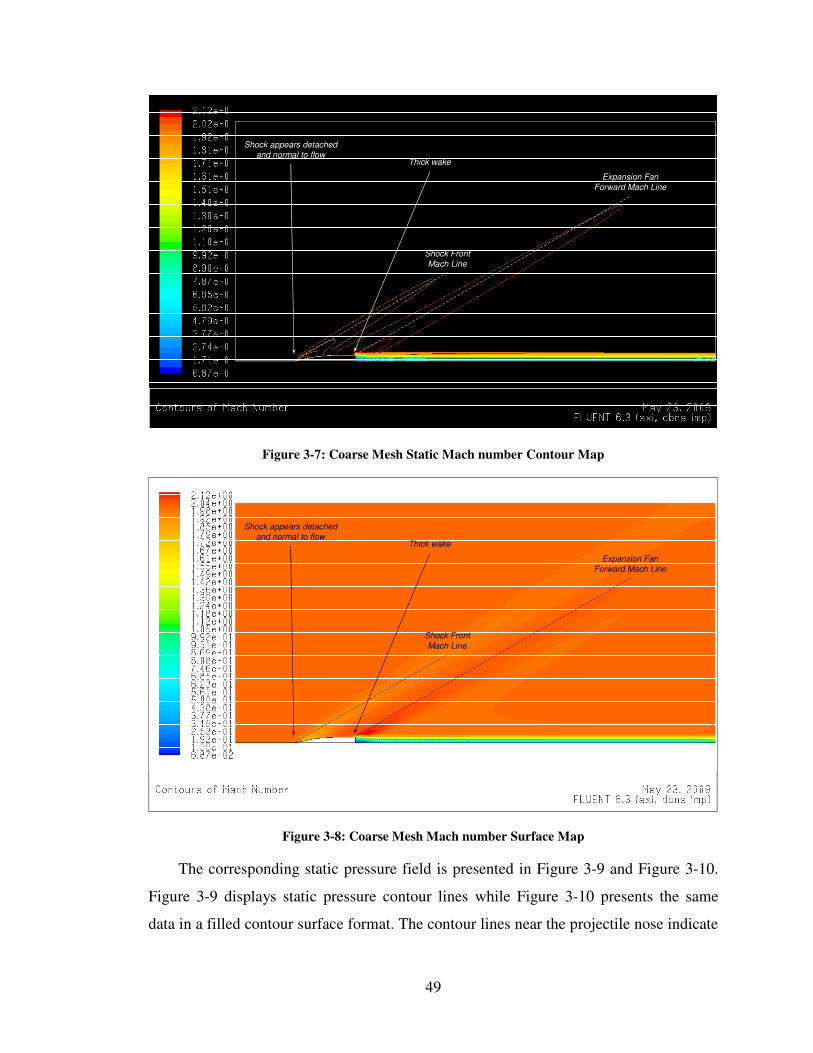
49

NACA Report 1122, No. 24 Shape

Shock appears detached

and normal to flowThick wake

Shock Front

Mach Line

Expansion Fan

Forward Mach Line

Figure 3-7: Coarse Mesh Static Mach number Contour Map



Shock Front

Mach Line

Expansion Fan

Forward Mach Line

Figure 3-8: Coarse Mesh Mach number Surface Map

The corresponding static pressure field is presented in Figure 3-9 and Figure 3-10.

Figure 3-9 displays static pressure contour lines while Figure 3-10 presents the same

data in a filled contour surface format. The contour lines near the projectile nose indicate

50

a gradient that forms an angle to the projectile axis that is similar to the MoC shock front

Mach line. The gradient angle is greater than the shock front Mach line angle and curved

near the projectile nose. As with the Mach number figures, close examination of the

gradients at the nose suggest that the shock is detached, forward of the projectile and

normal to the inflow velocity vector. The static pressure immediately behind the shock

front increases and appears to return to the inflow condition near the projectile base. The

static pressure decreases steadily throughout the region adjacent to the ogive and into the

region adjacent to the body. The static pressure has nearly returned to the inflow static

pressure at the transition to region 3. The base expansion is not well defined because the

contours that run parallel to the MoC Mach line extend forward of the projectile base.



Shock Front

Mach Line

Expansion Fan

Forward Mach Line

Figure 3-9: Coarse Mesh Pressure Contour Map

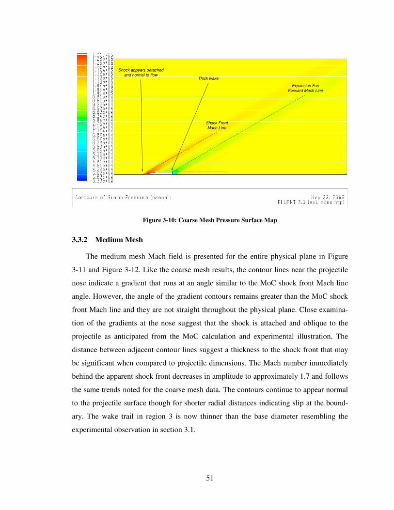
51



Shock Front

Mach Line

Expansion Fan

Forward Mach Line

Figure 3-10: Coarse Mesh Pressure Surface Map

3.3.2 Medium Mesh

The medium mesh Mach field is presented for the entire physical plane in Figure

3-11 and Figure 3-12. Like the coarse mesh results, the contour lines near the projectile

nose indicate a gradient that runs at an angle similar to the MoC shock front Mach line

angle. However, the angle of the gradient contours remains greater than the MoC shock

front Mach line and they are not straight throughout the physical plane. Close examina-

tion of the gradients at the nose suggest that the shock is attached and oblique to the

projectile as anticipated from the MoC calculation and experimental illustration. The

distance between adjacent contour lines suggest a thickness to the shock front that may

be significant when compared to projectile dimensions. The Mach number immediately

behind the apparent shock front decreases in amplitude to approximately 1.7 and follows

the same trends noted for the coarse mesh data. The contours continue to appear normal

to the projectile surface though for shorter radial distances indicating slip at the bound-

ary. The wake trail in region 3 is now thinner than the base diameter resembling the

experimental observation in section 3.1.

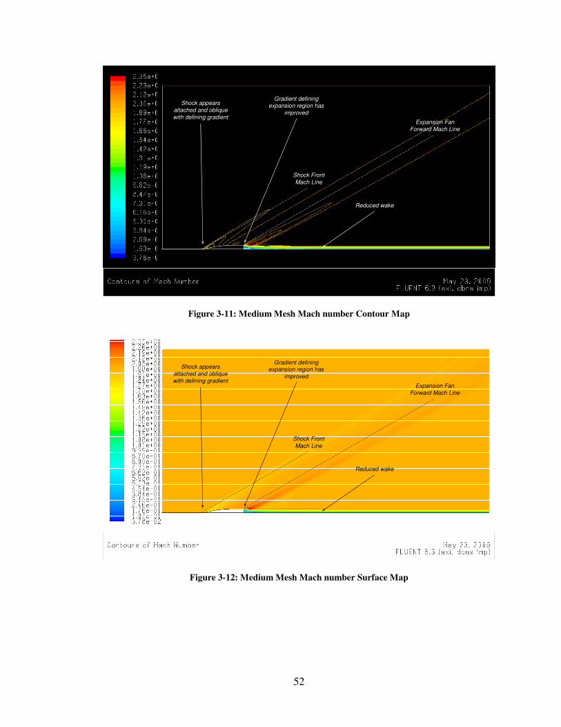
52


Shock appears

attached and oblique

with defining gradient

Gradient defining expansion region has

improved

Shock Front

Mach Line

Expansion Fan

Forward Mach Line

Reduced wake

Figure 3-11: Medium Mesh Mach number Contour Map

Shock appears




improved

Shock Front

Mach Line

Expansion Fan

Forward Mach Line

Reduced wake

Figure 3-12: Medium Mesh Mach number Surface Map

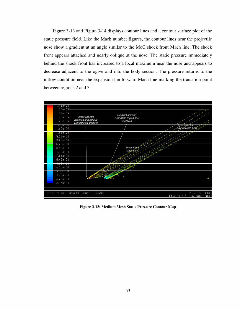
53

Figure 3-13 and Figure 3-14 displays contour lines and a contour surface plot of the

static pressure field. Like the Mach number figures, the contour lines near the projectile

nose show a gradient at an angle similar to the MoC shock front Mach line. The shock

front appears attached and nearly oblique at the nose. The static pressure immediately

behind the shock front has increased to a local maximum near the nose and appears to

decrease adjacent to the ogive and into the body section. The pressure returns to the

inflow condition near the expansion fan forward Mach line marking the transition point

between regions 2 and 3.

Shock appears




improved

Shock Front

Mach Line

Expansion Fan

Forward Mach Line

Figure 3-13: Medium Mesh Static Pressure Contour Map

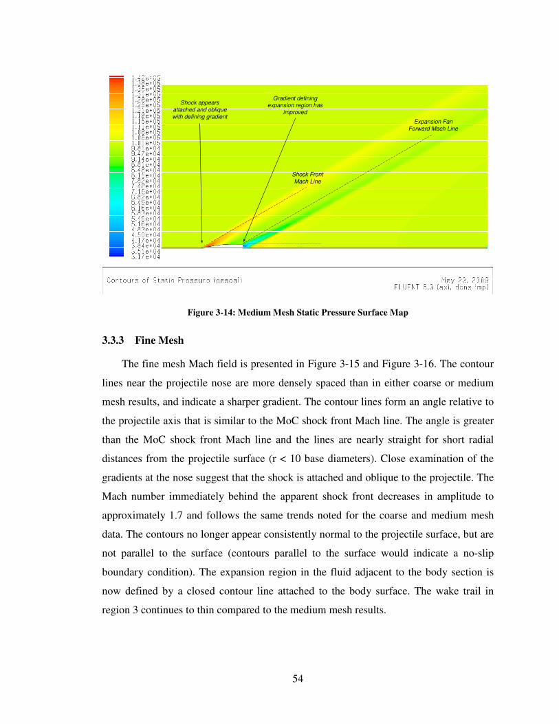
54

Shock appears




improved

Shock Front

Mach Line

Expansion Fan

Forward Mach Line

Figure 3-14: Medium Mesh Static Pressure Surface Map

3.3.3 Fine Mesh

The fine mesh Mach field is presented in Figure 3-15 and Figure 3-16. The contour

lines near the projectile nose are more densely spaced than in either coarse or medium

mesh results, and indicate a sharper gradient. The contour lines form an angle relative to

the projectile axis that is similar to the MoC shock front Mach line. The angle is greater

than the MoC shock front Mach line and the lines are nearly straight for short radial

distances from the projectile surface (r < 10 base diameters). Close examination of the

gradients at the nose suggest that the shock is attached and oblique to the projectile. The

Mach number immediately behind the apparent shock front decreases in amplitude to

approximately 1.7 and follows the same trends noted for the coarse and medium mesh

data. The contours no longer appear consistently normal to the projectile surface, but are

not parallel to the surface (contours parallel to the surface would indicate a no-slip

boundary condition). The expansion region in the fluid adjacent to the body section is

now defined by a closed contour line attached to the body surface. The wake trail in

region 3 continues to thin compared to the medium mesh results.

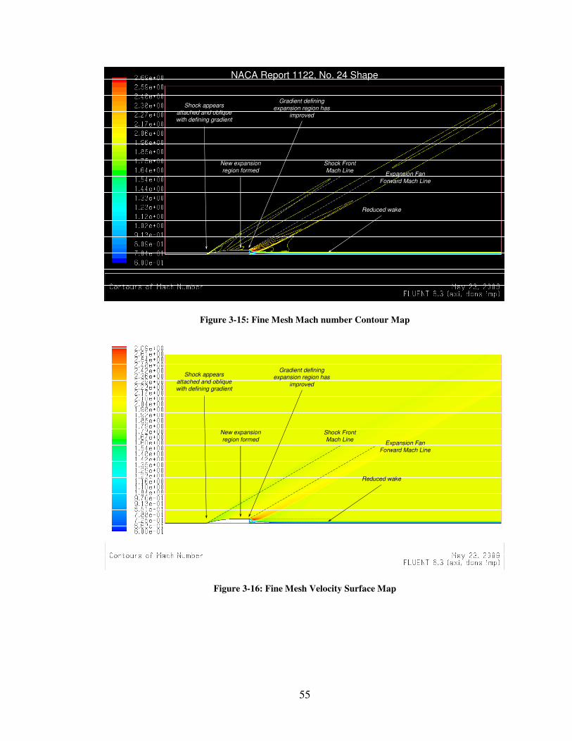
55


Shock appears

attached and obliquewith defining gradient

Gradient defining

expansion region has improved

Shock Front

Mach LineExpansion Fan

Forward Mach Line

Reduced wake

New expansion

region formed

Figure 3-15: Fine Mesh Mach number Contour Map

Shock appears



improved


Expansion FanForward Mach Line

Reduced wake

New expansion

region formed

Figure 3-16: Fine Mesh Velocity Surface Map

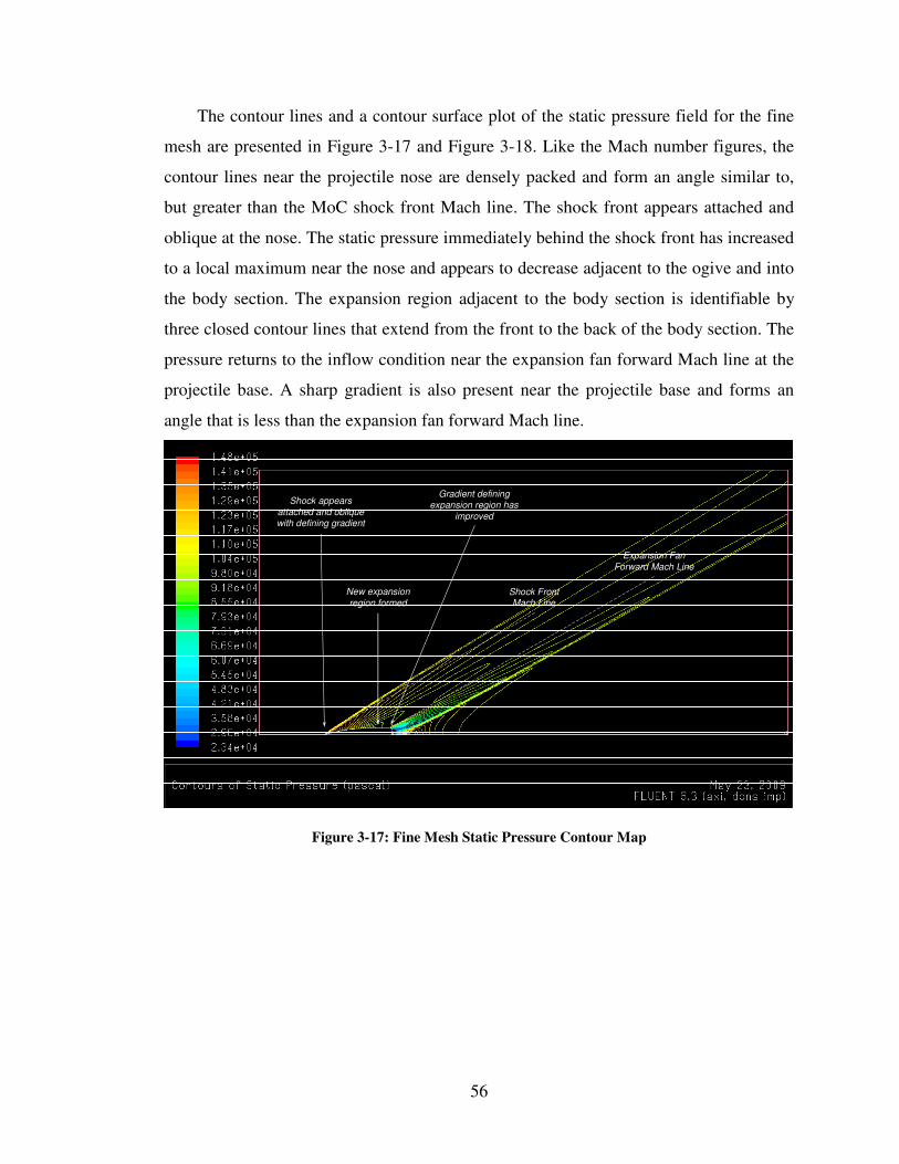
56

The contour lines and a contour surface plot of the static pressure field for the fine

mesh are presented in Figure 3-17 and Figure 3-18. Like the Mach number figures, the

contour lines near the projectile nose are densely packed and form an angle similar to,

but greater than the MoC shock front Mach line. The shock front appears attached and

oblique at the nose. The static pressure immediately behind the shock front has increased

to a local maximum near the nose and appears to decrease adjacent to the ogive and into

the body section. The expansion region adjacent to the body section is identifiable by

three closed contour lines that extend from the front to the back of the body section. The

pressure returns to the inflow condition near the expansion fan forward Mach line at the

projectile base. A sharp gradient is also present near the projectile base and forms an

angle that is less than the expansion fan forward Mach line.

Shock appears



improved


Expansion Fan

Forward Mach Line

New expansion

region formed

Figure 3-17: Fine Mesh Static Pressure Contour Map

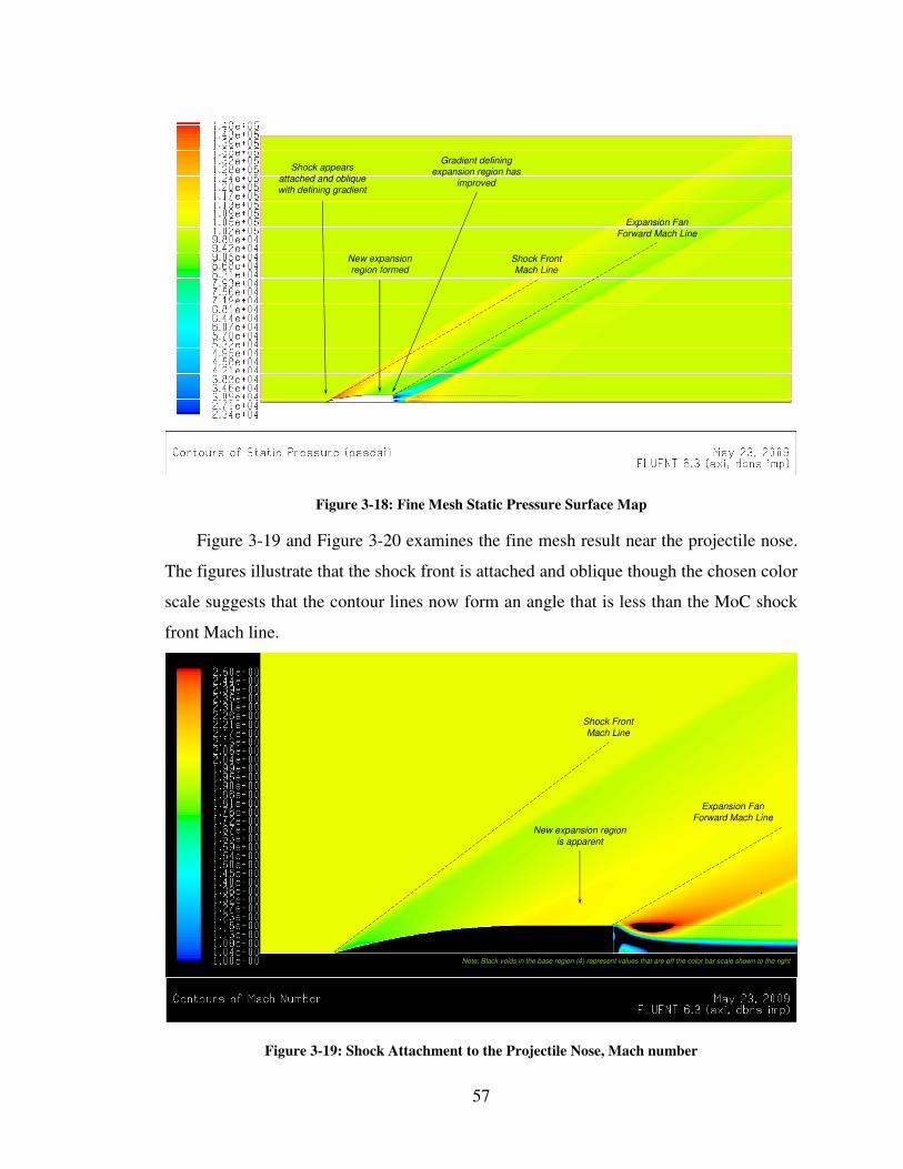
57

Shock appears



improved


Expansion Fan

Forward Mach Line

New expansionregion formed

Figure 3-18: Fine Mesh Static Pressure Surface Map

Figure 3-19 and Figure 3-20 examines the fine mesh result near the projectile nose.

The figures illustrate that the shock front is attached and oblique though the chosen color

scale suggests that the contour lines now form an angle that is less than the MoC shock

front Mach line.

Shock Front

Mach Line

Expansion Fan

Forward Mach Line

Note: Black voids in the base region (4) represent values that are off the color bar scale shown to the right

New expansion region

is apparent

Figure 3-19: Shock Attachment to the Projectile Nose, Mach number

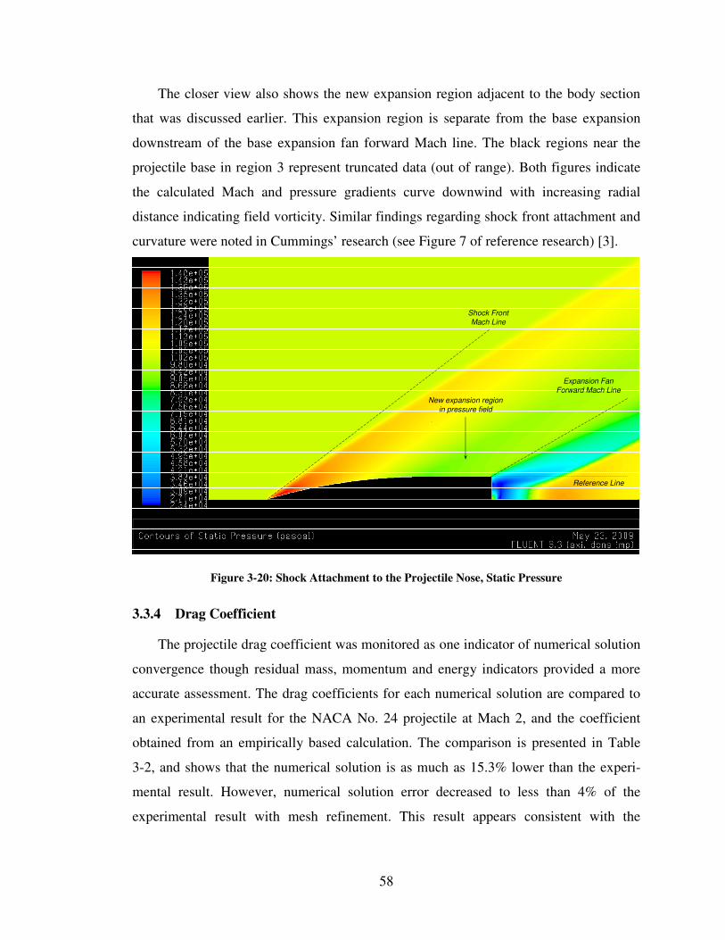
58

The closer view also shows the new expansion region adjacent to the body section

that was discussed earlier. This expansion region is separate from the base expansion

downstream of the base expansion fan forward Mach line. The black regions near the

projectile base in region 3 represent truncated data (out of range). Both figures indicate

the calculated Mach and pressure gradients curve downwind with increasing radial

distance indicating field vorticity. Similar findings regarding shock front attachment and

curvature were noted in Cummings’ research (see Figure 7 of reference research) [3].

Shock Front

Mach Line

Expansion Fan

Forward Mach Line

Reference Line

New expansion region

in pressure field

Figure 3-20: Shock Attachment to the Projectile Nose, Static Pressure

3.3.4 Drag Coefficient

The projectile drag coefficient was monitored as one indicator of numerical solution

convergence though residual mass, momentum and energy indicators provided a more

accurate assessment. The drag coefficients for each numerical solution are compared to

an experimental result for the NACA No. 24 projectile at Mach 2, and the coefficient

obtained from an empirically based calculation. The comparison is presented in Table

3-2, and shows that the numerical solution is as much as 15.3% lower than the experi-

mental result. However, numerical solution error decreased to less than 4% of the

experimental result with mesh refinement. This result appears consistent with the

59

inviscid assumption given the observation that the drag coefficient is predominantly

determined by base drag [5].

Table 3-2: Drag Coefficient Comparison

Source Drag Coefficient (Cd) Error (%)1

Experimental Result [2] ~0.2202 -

Empirical Data Fit (base only) [5] ~0.2166 -1.63

Coarse Mesh Numerical Result 0.1865 -15.30

Medium Mesh Numerical Result 0.1879 -14.67

Fine Mesh Numerical Result 0.2117 -3.86

1 – Error is calculated as variation relative to the experimental result without consideration to experimental error

An additional drag coefficient comparison is performed using the inverse of the

Mach number squared to approximate the coefficient [3]. This approximation is gener-

ally valid at higher Mach numbers and yields a drag coefficient of 0.25 that is similar to

the values in Table 3-2.

60

4. Conclusions

Comparisons between the MoC and numerical solutions show that both methods

capture the shape and oblique angle characteristics of the projectile nose shock. How-

ever, the MoC solutions do not indicate vorticity across the shock due to the application

of additional isentropic fluid assumptions. The numerical solutions included vorticity as

indicated by the curvature of the shock front, but did not adequately represent the fluid

gradients across the shock front for the three mesh densities that were evaluated. There-

fore the shock front exhibited thickness that was orders of magnitude greater than the

molecular mean free path. Additional key findings are summarized below.

• The numerical solutions indicate that the shock front converges to a straight line for

a short radial distance near the projectile nose. Comparisons to oblique shock or is-

entropic flow relations and the MoC solution show the minimum fluid speed (or

maximum pressure is achieved in this region of the flow field.

• The numerical solutions predict a weak fluid expansion adjacent to the cylindrical

projectile body section. The prediction trend is consistent with other research and

experimental data, but is not apparent in the MoC solution (due to the isentropic as-

sumption) or experimental illustration presented herein.

• The expansion region downstream of the shock is distributed over the entire axial

length of the tangent ogive and prevents the formation of a strong expansion further

downstream. This finding is supported by both MoC and numerical solutions, and

explains why the tangent ogive is preferred over conical shapes that are easier to

manufacture.

Several conclusions can be drawn regarding the complexity of implementing the

MoC and numerical solutions. The MoC solution poses significant implementation

difficulty due to partitioning of the physical plane into separate regions and irregular

spacing of characteristic net intersection points. Each region requires modified solution

steps to transfer the boundary conditions into the flow field, and the sharp corner at the

projectile base must be treated as a small radial arc with very fine mesh point density to

obtain sufficient characteristic line intersection points in the strong expansion region

61

downstream of the projectile. The technique is not easily adapted to operate over a wide

range of fluid dynamic problems for the same reasons. Once implemented, the calcula-

tions are completed in less computation time compared to numerical approaches. The

partial MoC solution consisting of the shock front location, angle of the shock or projec-

tile surface Mach number are obtained with less effort and offer a reasonable measure to

evaluate numerical model mesh adequacy.

The numerical method exhibited different implementation difficulties in that experi-

ence with a broader range of mathematic (numerical) techniques is needed to obtain a

converging solution. Experience demonstrated that convergence is not sufficient to

ensure accurate results, and the analyst may iteratively revise the numerical model mesh

to capture the desired field characteristics. The numerical solution offered a substantial

advantage in terms of completeness since it did not require the isentropic or irrotational

assumption for implementation. Regardless of analysis method used, a comparison to

experimental data is a prudent step toward calculation verification.

Though not a specific objective of this study, it is interesting to note that the nu-

merical solutions calculated a drag coefficient that was only 4% lower than previously

reported experimental data even though viscous effects were neglected. The drag coeffi-

cient is predominantly dependent of the projectile base drag (a fluid region that was not

evaluated with the MoC).

62

5. Areas for Future Work

The supersonic external ballistics problem offers significant challenges with regard

to the estimation of fluid Mach and pressure fields near the projectile. Many of these

challenges could not be addressed in this study and afford areas of future work. Some of

these areas were mentioned in appropriate sections of the study and are summarized

below.

• The pressure fields should be recalculated in terms that are readily compared rather

than the pressure ratio from the MoC solution and the numerical solution static pres-

sure values.

• The MoC solution should be expanded to evaluate flow downstream of the base.

• Further numerical mesh refinements should be implemented to improve the solution

near the projectile nose.

• The solution methods should be expanded to incrementally removed simplifying

assumptions and include viscous effects.

63

6. References

[1] Anderson, J. D. Modern Compressible Flow with Historical Perspective

[ISBN 007-124136-1]. New York: McGraw-Hill, 2003.

[2] Walchner, O. "Systematic Wind Tunnel Measurements on Missiles." National

Advisory Committee for Aeronautics Technical Memorandum No. 1122 (1947): 13.

[3] Cummings, R. M., H. T. Yang, and Y. H. Oh. "Supersonic Turbulent Flow Compu-

tation and Drag Optimization for Axisymmetric Afterbodies." Computers and

Fluids 24, no. 4 (1995): 487-507.

[4] Garibaldi, Javier, Mario Storti, Laura Battaglia, and Jorge D’El´ıa. "Numerical

simulations of the flow around a spinning projectile in subsonic regime." Instituto

de Investigaciones Cient´ıficas y T´ecnicas de las Fuerzas Armadas (CITEFA) Re-

port No. 1040 (2007): 18.

[5] McCoy, Robert L.. "MC Drag - A Computer Program for Estimating the Drag

Coefficients of Projectiles." U.S. Army Armament Research & Development

Command Report No. ARBRL-TR-02293 (1981): 74.

[6] Takakura, Yoko, F. Higashino, S. Ogawa. "Unsteady Flow Computations on a

Flying Projectile within a Ballistic Range." Computers and Fluids 27, No. 5-6

(645-650): 1998.

[7] Department of the Army – Development and Readiness Command (DARCOM),

"LOGISTICS COMPLETE ROUND CHARTS AMMUNITION THROUGH 30

MILLIMETERS." Published May 31, 1984. http://www.fas.org/man/dod-

101/sys/land/docs/p700_3_2.pdf (accessed 16 May 2009).

[8] Hawks, Chuck. "Rifle Ballistics Summary." 2006.

http://www.chuckhawks.com/rifle_ballistics_table.htm (accessed April 24, 2009).

[9] Department of the Army – Army Material Command (AMC), "ARTILLERY

AMMUNITION." Published November 30, 1985. http://www.fas.org/man/dod-

101/sys/land/docs/p700_3_3.pdf (accessed 16 May 2009).

[10] Tannehill J. C., D. A. Anderson, R. H. Pletcher. Computational Fluid Mechanics

and Heat Transfer [ISBN 1-56032-046-X]. Philadelphia: Taylor & Francis, 1997.

[11] Fluent 6.2 User's Manual. Volume 1, Lebannon, NH: Fluent Incorporated, 2005.

[12] Ferri, Antonio. "The Linearized Characteristics Method and Its Application to

Practical Nonlinear Supersonic Problems." National Advisory Committee for Aero-

nautics Technical Memorandum No. 1102 (1952): 18.

64

[13] Griffing, C. W., W. Wilburn, D. Purdon, E. McLaughlin. “An Application of the

Method of Characteristics to Axially Symmetric Supersonic Flow.” California In-

stitute of Technology Thesis (1947): 49.

[14] Ferri, Antonio. "The Method of Characteristics for the Determination of Super-

sonic Flow Over Bodies of Revolution at Small Angles of Attack." National

Advisory Committee for Aeronautics Technical Memorandum No. 1044 (1951): 18.

[15] Ferri, Antonio. “Application of the Method of Characteristics to Supersonic

Rotational Flow.” National Advisory Committee for Aeronautics Technical Memo-

randum No. TR-841 (1946): 12.

[16] Gambit 2.2 Tutorial Guide. Volume 1, Lebannon, NH: Fluent Incorporated, 2004.

[17] Fluent 6.2 Tutorial Guide. Volume 1, Lebannon, NH: Fluent Incorporated, 2005.

Documents

Method of Characteristics and Numerical Solutions for the Supersonic External Ballistics Problem