A description of numerical methods and computer programs ... · PDF filecomputer programs for two-dimensional and axisymmetric supersonic flow ... and axisymmetric supersonic flow

NASA TECHNICAL NOTE NASA TN D-2970 -

4. / . - -

A DESCRIPTION OF NUMERICAL METHODS AND COMPUTER PROGRAMS FOR TWO-DIMENSIONAL A N D AXISYMMETRIC SUPERSONIC FLOW OVER BLUNT-NOSED A N D FLARED BODIES

by M L Z ~ O Y U Iaonye, John V. R ~ k k h , dad Harvmd L O ~ U X

Ames Reseurch Center M o ffett Field, Cu Zz?

NATIONAL AERONAUTICS AND SPACE ADMINISTRATION 0 WASHINGTON, D. C. AUGUST 1965

TECH LIBRARY KAFB. NY

0079963

A DESCRIPTION OF NUMERICAL METHODS AND COMPUTER PROGRAMS

FOR TWO-DIMENSIONAL AND AXISYMMETWC SUPERSONIC FLOW

OVER BLUNT-NOSED AND FLARED BODIES

By Mamoru Inouye, John V. Rakich, and Harvard Lomax

Ames Research Center Moffett Field, Calif.

NATIONAL AERONAUTICS AND SPACE ADMINISTRATION . .

For sale by the Clearinghouse for Federa l Scientif ic and Technical Information Springfield, V i rg in ia 22151 - Pr ice $2.00

A DESCRIPTION O F NUMERICAL METHODS AND COMPUTER PROGRAMS

FOR TWO-DIMENSIONAL AND AXISYMMETRIC SUPERSONIC FLOW

OVER BLUNT-NOSED AND F!LA€BD BODIES

By Mamoru Inouye, John V. Rakich, and Harvard Lomax Ames Research Center

SUMMARY

The computer programs developed a t Ames Research Center f o r calculat ing the inviscid flow f i e l d around blunt-nosed bodies a r e described b r i e f l y and t h e i r appl icat ion 'to spec i f ic shapes i s demonstrated. The programs solve numerically the exact equations of motion fo r plane o r axisymmetric bodies a t zero angle of a t tack and f o r a perfect gas or a r e a l gas i n thermodynamic equilibrium. A n inverse method i s used fo r the subsonic-transonic region, and the method of charac te r i s t ics i s used f o r t he supersonic region. Results a r e shown f o r several body shapes i n both perfect and r e a l gas flow, including a comparison between air and a C02-N2 mixture. Presented a re shock-wave shapes and d is t r ibu t ions of pressure and other flow variables along the body and across the shock l aye r .

INTRODUCTION

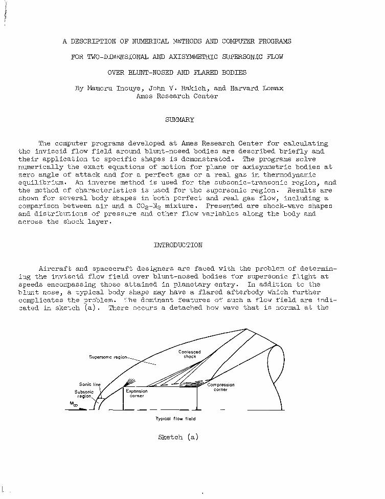
Aircraf t and spacecraft designers a re faced with the problem of determining the inviscid flow f i e l d over blunt-nosed bodies f o r supersonic f l i g h t a t speeds encompassing those a t ta ined i n planetary entry. In addition t o the blunt nose, a typ ica l body shape may have a f l a r ed afterbody which fur ther complicates the problem. The dominant features of such a f l o w f i e l d a re indicated in sketch ( a ) . There occurs a detached bow wave tha t i s normal a t the

Supersonic region

Typical f low field

Sketch (a)

axis of symmetry and decays i n s t rength as it approaches a Mach wave a t la rge distances from the body. The f l o w behind the shock wave i s subsonic i n the nose region bounded by the sonic l i n e and becomes supersonic over the a f te r - body. Expansion waves and embedded shocks may occur as a r e s u l t of corners. In addi t ion, an embedded shock may a r i s e from coalescence of compression waves from the surface o r from separation of t he boundary layer , which of ten occurs on t h i s type of body. Analysis of t he viscous region i s beyond the scope of the present study; however, i t s study depends on a knowledge of the external inviscid flow.

A nuniber of exact and approximate techniques f o r determining the f l o w Some of the more recent con- f i e l d depicted i n sketch (a) have been reported.

t r ibu t ions are references 1 through 4 f o r blunt-body flows, and references 5 and 6 f o r the supersonic region downstream of the nose. For f l a r ed bodies, exact numerical results have been reported i n reference 7 while approximate methods may be found i n references 8 through 10. present a more complete discussion of the e n t i r e flow f i e l d .

Hayes and Probstein ( r e f . 11)

The computer programs t h a t a r e described i n the present report solve numerically the exact equations of motion f o r plane and axisymmetric flow a t zero angle of a t t ack and provide the complete inviscid f l o w f i e l d between the body and the shock wave. The f l u i d may be a perfect gas o r a r e a l gas in thermodynamic equilibrium. An inverse method ( ref . 3) i s used f o r the subsonic-transonic region ( re fer red t o as the blunt-body program), and the method of cha rac t e r i s t i c s ( r e f . 5 ) i s used t o extend the calculations downstream i n the supersonic region. These computer programs were wri t ten in FORTRAN I1 f o r use on an IBM 7094 at Ames Research Center, but have been made avai lable t o a number of other organizations. The d i s t r ibu t ion of these programs has created a need f o r a more complete descr ipt ion and documentation than i s present ly avai lable . The present report i s intended t o p a r t i a l l y f u l f i l l t h i s need.

The purpose of the present report i s t o provide a general description of t he Ames flow-field computer programs and t o present r e s u l t s of calculations that demonstrate the range of app l i cab i l i t y . The governing equations of motion a re introduced b r i e f l y a t the start . Then the methods used t o solve the equations a re presented. of a l l the subroutines and flow charts . Instead, de ta i led descriptions a re provided only f o r selected portions of the programs t h a t warrant special con- s iderat ion. The information contained i n t h i s report should acquaint the reader with the general logic followed i n the programs and be helpful i n diagnosing small d i f f i c u l t i e s or i n making minor modifications.

No attempt i s made t o provide a complete l i s t i n g

Sample r e s u l t s a r e presented f o r shock-wave shape, surface-pressure d is t r ibu t ion , and shock-layer p ro f i l e s of t o t a l pressure, s t a t i c pressure, density, and ve loc i ty f o r various free-stream conditions and body shapes. The f i rs t examples demonstrate how a simple modification improves the accuracy of the calculat ions i n regions with la rge entropy (or vo r t i c i ty ) gradients . Then comparisons a re made with flow-field r e s u l t s obtained by means of an in tegra l method f o r t he blunt-body solut ion. Comparisons a re a l s o made with experimental r e s u l t s obtained f o r a body with a f lare. Finally, examples of calculations f o r r e a l gases i n thermodynamic equilibrium are presented.

2

SYMBOLS

a

h

ht

M

n

P

Pt

R

S

X

XYY

Y

n

6

E

speed of sound

ellipsoid bluntness, (b/c)2

semiaxes of ellipsoid

enthalpy

total enthalpy

Mach number

coordinate normal to a streamline

static pressure

total pressure

nose or cylinder radius

entropy

sheared coordinates (see eqs. (8))

velocity components in xyy directions

velocity

shock-wave shape

cylindrical coordinates with origin at body nose

ratio of specific heats

shock standoff distance

angle of corner on the body

index for number of degrees of symmetry; E = 0 for plane symmetric flow, and E = 1 for axisymmetric f l o w

flow angle

cone angle

Mach angle

3

p densi ty

$ stream function

Subscripts

b body

S shock

free-stream conditions

EQUATIONS

The p a r t i a l d i f f e r e n t i a l equations t h a t must be s a t i s f i e d f o r steady, inviscid flow a re as follows:

Continuity of mass

a € a E - (puy 1 + - (PVY 1 = 0 ax dY

where E = 0 f o r plane symmetric flow and E = 1 f o r axisymmetric flow.

Momentum equations

x d i rec t ion

dU du dP - d X dy dx

pu - + pv - + - - 0

y direct ion

a, a, dX dY S Y

pu - + pv - + 32 = 0

Energy equation

where a is the isentropic speed of sound defined by

(3)

(4)

a2 = (')s

4

( 5 )

To solve these equations f o r a given s e t of boundary conditions, the thermodynamic propert ies of the gas are required; f o r example,

a2 = f ( P , P )

For a perfect gas these relat ionships a re merely functions of the gas constant and r a t i o of spec i f ic heats . For example, equation (6) becomes

For a r e a l gas the equilibrium composition and thermodynamic propert ies must be obtained by means of s t a t i s t i c a l mechanics. These calculations can be done independently of the flow-field equations, and the r e su l t s can be tabulated f o r l a t e r use. D r . Harry E. Bailey of Ames Research Center has recent ly per- formed these calculat ions f o r various gas mixtures of current i n t e re s t following the assumptions and approximations made by Marrone (ref. 12) . cover temperatures t o 25,OOOO K i n 250' increments and dens i t ies from lo3 times a reference density, po, which i s the densi ty of the mixture f o r a temperature of 273.16' K and a pressure of 0.101325 MN/m2 (1 atmosphere). For example, the propert ies f o r carbon dioxide are reported i n reference 13.

The data t o

The thermodynamic propert ies i n t h i s form a r e not sui table f o r optimal use i n a computer program. Some approximations a re necessary t o minimize the computing time and storage requirements. For use i n the present programs, the calculated values of the propert ies have been spl ine f i t t e d with cubics by the method of reference 14, and the coef f ic ien ts of the cubics have been stored on magnetic tape. A special subroutine reads the tape, searches fo r the proper coeff ic ients , and evaluates the desired propert ies . This approximate technique,in general, y ie lds results within 1 percent of the or ig ina l data . A t present the thermodynamic propert ies fo r air and the twelve mixtures of n i t ro- gen, carbon dioxide, and argon l i s t e d i n t a b l e I are avai lable on tape .

For moderate temperatures, f o r example, below about 2000° K f o r a i r , dissociat ion and ionizat ion can be neglected, and the imperfect gas e f f ec t s a r e due t o the exci ta t ion of the v ibra t iona l s t a t e s . The thermodynamic prop- e r t i e s fo r such thermally perfect gases have been calculated i n reference 15 and have a l so been stored on tape f o r use i n the present programs.

The system of equations i s now complete. In general, t he four p a r t i a l d i f f e r e n t i a l equations (eqs. (1) through ( 4 ) ) must be solved simultaneously f o r the four dependent var iables p,p,u, and v . I n the following sections the methods used t o solve these equations numerically i n the subsonic- transonic region and i n the supersonic region a re discussed.

METHOD O F SOLUTION FOR SUBSONIC-TRANSONIC REGION

In the nose region of blunt bodies, equations (1) through (4) exhibi t d i f f e ren t character; namely, t he equations a re e l l i p t i c i n the subsonic region,

5

parabolic on the sonic l i n e , and hyperbolic i n the supersonic region. these complications, an inverse method (see, e.g. , r e f . 1) has been found e f f ec tua l f o r solving such flow f i e l d s . shock shape i s assumed and the equations a re integrated numerically by a f ini te-difference method t o determine the corresponding body shape. t i c u l a r version used i n t h i s report i s reported in d e t a i l i n reference 3; hence, only a b r i e f descr ipt ion w i l l follow.

Despite

I n the appl icat ion of t h i s method, a

The par-

Since the i n i t i a l boundary conditions a re specified along the shock, a sheared, nonorthogonal coordinate system with one axis coincident with the shock i s useful (see sketch (b)). The new coordinates a re defined as follows:

Sketch (b)

I s = x - x(y)

t = y

Equations (1) through (4) a r e then transformed and expressed in the following form:

2Q = 'F,(t,P,P,U,V, -, aP - dP, a,, 9 I 3, a t a t a t a

} (9) 22- = (P3(t?P?P?U?V? - aP, a,, a,, *)

a t a t a t a t as

For a given s e t of free-stream conditions and shock shape, the values of p,p,u, and v/ t Hugoniot Telations, and the der ivat ives with respect t o t a re found by numerical d i f f e ren t i a t ion . s tep toward the body. A flow chart f o r the computer program i s shown i n f igure 1, and a l i s t of subroutines i s provided i n t ab le 11. To i l l u s t r a t e the predictor-corrector integrat ion technique, suppose the flow propert ies a re known f o r the (i - 1 ) t h and i t h s teps and a re t o be calculated f o r the (i + 1 ) t h s tep (see sketch ( b ) ) . A second-order predictor and a modified Eulerian second-order corrector a re used as follows, where p i s a typ ica l flow variable .

j u s t behind the shock wave are calculated from the Rankine-

Then equations (9) a re used t o march i n step-by-

1. Different ia te numerically data f o r i t h s tep t o obtain (a,/&), 2 . Calculate from equations (9), ( a p / a ~ ) ~

6

i - - + 2 as(ap/as) P i - 1 3. Predict new value pi+l

4.

5 .

6.

Different ia te numerically t o obtain (ap/at)

Calculate from equations (9) , (@/as) i+l

Correct value pi+l = pi + 0.3 ~ ~ [ ( a p / a s ) ~ + ( a P / a ~ ) ~ + ~ l

The stream function i s calculated f o r each point, and the body i s determined as the locus of points where the stream function vanishes. Tne s tep s i ze i s chosen so tha t the stagnation point i s reached i n approximately seven s teps . It i s usually necessary t o i t e r a t e on the shock shape t o obtain the desired body shape. However, t h i s procedure i s simplified by a one-parameter family of shock shapes t h a t w i l l produce reasonably accurate spheres and e l l i p so ids . Values of the shock-shape parameter fo r spheres a re presented i n reference 3 f o r perfect gases and f o r a i r i n thermodynamic equilibrium. Solu- t i ons f o r other gases and nonspherical bodies including not-too-blunt e l l i p - soids can be obtained by appropriate changes of the shock-shape parameter. There a re l imi ta t ions on the appl icat ion of the program, mainly because of inherent numerical d i f f i c u l t i e s , as discussed i n reference 3. A s a general ru le , solutions a re not possible f o r Mach numbers l e s s than 3 and f o r body shapes tha t a re e i t h e r very blunt (% > 4) o r not smooth i n the nose region.

The output from the blunt-body program consis ts of the f l o w propert ies on

In addition, the propert ies a re interpolated along a l i n e joining the body and i n the flow f i e l d a t the coordinate intersect ions shown in sketch ( b ) . the shock and body i n the supersonic region. These.data can be used as input fo r the method of charac te r i s t ics program t o continue the calculat ions downstream over the afterbody.

METHOD O F SOLUTION FOR SUPEESONIC REGION

A computer program based on the method of charac te r i s t ics i s used t o determine the flow f i e l d i n the supersonic region. This program is comprised of a main program and 33 subroutines which a re l i s t e d i n t ab le 111. Most of these subroutines a re short and straightforward and, therefore, they w i l l not be explained in d e t a i l . (Table I11 describes the primary function of each.) However, t he main program requires a few words of explanation. In addition, cer ta in quadratic interpolat ion procedures as well as methods f o r calculating embedded shock waves w i l l be discussed.

Calculation Procedure f o r Smooth Bodies

Along the charac te r i s t ic or Mach l i n e s , the p a r t i a l d i f f e r e n t i a l equa- t i ons ((1) through (3 ) ) reduce t o the following ordinary equations (see, e.g., r e f . 11):

7

Equation (10) is solved i n conjunction with the energy equation i n integrated form

F h + - = h t = constant 2

the conservation of entropy on streamlines

and the equation of s t a t e

Briefly, the method consis ts of s t a r t i ng with flow propert ies along a non- charac te r i s t ic l i n e between the body and the shock wave, as determined from the solution fo r the subsonic-transonic region, and then integrat ing the equations downstream along the Mach l i n e s . t r a t e d by the typ ica l charac te r i s t ic mesh shown i n sketch ( e ) .

The stepwise procedure i s i l lus- Beginning with

known data on the s t a r t i ng l i n e the calculat ion proceeds t o the body along a right-running

t o the next s t a r t i ng point (or

chart i s shown i n f igure 2

the program log ic . In sketch sketch ( e ) , the previously calculated (or input) data points a r e ident i f ied by small c i r c l e s , and the point current ly being

Current data is stared in array, P (J, K ),

J - identifies flow charac te r i s t ic , and then back variables (x, y, V,-- etc) K - identifies the location of the field points shock po in t ) . A simple flow (numbered as shown)

Direction of calculation which i l l u s t r a t e s t h i s par t of

Typical characteristic mesh

I X calculated i s ident i f ied by the shaded symbol. Only the nun- bered points are avai lable in

Sketch ( e ) computer memory a t t h i s time, the remaining c i rc led points having been wri t ten out pre-

viously. P(J,K), i n which the index, J iden t i f i e s the various flow variables and the index K i den t i f i e s the locat ion of the point . In terms of program termin- ology, the number of f i e l d points involved i n the calculat ion loop is given by M2 + 1, where I@ i s an integer defined i n the main program. The f i e l d point current ly being calculated is ident i f ied as P(J,K9), where Kg i s a l so an integer defined i n the main program. along a right-running charac te r i s t ic , the integer Kg takes on successive values between Kg = M2 + 1 on the shock (o r input l i n e ) t o Kg = 1 on the

The stored data points a re contained i n a two-dimensional array,

Thus as the calculat ion proceeds

’ body.

For the calculat ion of a typ ica l mesh point (C i n sketch ( e ) ) , three adjacent points a r e usually used. These points are labeled A,D,B i n sketch ( e ) , and correspond, i n the example shown, t o the points K = 2,3,4 in

8

the P array. The calculat ion of data a t the new point i s effected with the use of equations (10) through (13) and a standard predictor-corrector procedure which averages the coef f ic ien ts of the d i f f e r e n t i a l s . The procedure i s s t a r t ed with a crude predictor ( i . e . , t h a t conditions a t equal those a t B) and i s followed, therefore , by a t l e a s t two correctors . This i s i n con- t ras t t o the method used f o r the blunt-body solution which makes use of only one corrector, but which uses a second-order predictor .

C

In calculat ing ro t a t iona l supersonic flow by the method of characteris- t i c s , it i s convenient t o introduce entropy as a flow property since it remains constant on streamlines. In the past it has sometimes been assumed tha t the entropy var ies l i n e a r l y between streamlines (see ref. 16, p . 636). To i l l u s t r a t e t h i s procedure, consider three points i n the flow f i e l d (see sketch ( c ) ) A and B, where the flow propert ies are known, and C, where the flow propert ies are t o be determined. The entropy a t C can be calculated using the flow propert ies a t A and B and with the assumption t h a t the entropy var ies l i n e a r l y along the normal t o the streamlines between A and B. This assumption i s va l id provided t h a t the change in entropy gradient between A and B i s small. However, serious e r r m s may occur in the flow-field calculations i f t h i s condition i s not rea l ized (see, e .g . , r e f . 17). Decreasing the mesh s ize by increasing the number of mesh points i s not a sa t i s f ac to ry remedy because the computing time increases as the square of the number of input points, and the storage capacity of computing machines i s a l s o l imited. In reference 1.7, an i t e r a t i v e scheme w a s used wherein a check on the integrated mass f l o w was made point by point throughout the f i e l d . The method adopted i n the present program i s simpler i n t h a t no addi t ional i t e r a t ions a re needed. Quadratic ra ther than l i n e a r interpolat ion f o r the entropy is used, and er rors a re therefore reduced t o the order of t he cube of the mesh s i z e . This i s accomplished by using the flow propert ies a t point D, which l i e s on Mach l i n e s upstream from A and B. This addi t ional point allows the use of a quadratic calculat ion f o r entropy between A and B. Some improvement i n the flow-field solution can be expected, especial ly in regions where la rge changes i n entropy gradient occur.

A feature of the present computer program, which proved useful fo r exam- ining entropy gradients, i s the a b i l i t y t o in te rpola te f o r f i e l d data on r a d i a l (body- o r axis-normal) l i n e s . chart ( f i g . 2 ) . These interpolated data a t several x s t a t ions are pr inted out a t the end of the normal output and, i f desired, the data from the las t x s t a t ion can be stored on magnetic tape. This tape can l a t e r be used t o provide s t a r t i ng conditions t o extend the calculat ion downstream.

This operation is noted i n the flow

Calculation Procedure f o r Bodies With Corners

The method of charac te r i s t ics described i n the previous sect ion i s not applicable i n regions where the body slope i s discontinuous, o r where embedded shocks occur. For these cases, charac te r i s t ics theory may be applied on both s ides of the discont inui ty with matching conditions obtained f o r the Rankine- Hugoniot shock re la t ions , o r Prandtl-Meyer equations i n the case of an expansion corner. Methods f o r calculat ing flows of t h i s type may be found, f o r

9

example, in reference 16. calculation as incorporated into the present program.

This section describes some of the details of this

While any nwriber of discontinuities are allowable in theory, practical considerations have resulted in a limitation, for the present program, of any two of the discontinuities indicated in sketch (a). These are: sion corner, (b) a compression corner, and (c) an enibedded shock arising, for example, from a coalescence of Mach waves from a concave wall. Procedures used in calculating these three types of discontinuities are discussed next. Descriptions of the compression corner and coalesced shock explain only the starting conditions used for the shock calculation, and are followed by an explanation of a general embedded shock point. The calculation for an embedded shock proceeds to its intersection with the bow shock. Then, since inter- actions between shocks are not considered, the calculation terminates along a right-running characteristic through this point.

(a) an expan-

Expansion corner.- The expansion corner is illustrated in sketch (d). Upon reaching the body in region I1 for the first time, point C is calculated

on the extension of the body shape specified for region I. This pro- vides an analytic continuation of the flow ahead of the corner and, with stored data at points A and B, enables one to use a quadratic interpolation for conditions at point D just ahead of the corner. Now, given conditions at D and the expansion angle 6, the Prandtl-Meyer equations can be used to calculate conditions on the body just behind the corner. In addition, conditions for several intermediate angles are computed and all are stored with coordinate values corresponding to point D. The problem is now

With

Expansion w t w r

Sketch (a)

reduced to one which can be handled by the main characteristics program. known conditions at points D and E, point F can be computed, followed by similar calculations for points G,H, etc., until the entire expansion fan is determined as shown in the inset. A greater number of mesh points are introduced at such a corner for large expansion angles, so as to provide a reasonably uniform mesh.

Compression corner.- The compression corner is shown in sketch (e). procedure for calculating conditions at point D is identical with that described for the expansion corner. In. this case, the oblique shock relations are used to calculate the flow variables on the body just behind the corner in terms of upstream conditions at point D and the known deflection angle, 6. The necessary shock solution is not explicit, however, and an iterative procedure has been programmed to give the jump conditions. The segment of the shock D-F is assumed straight and at an angle corresponding to the oblique shock at point D. Data at point F are then found by a quadratic

10

The

Compression corner

Sketch ( e )

interpolat ion along the right-running charac te r i s t ic through E, and the jump conditions a t point F a re computed from the shock r e l a t ions . The data a t D ' and F' can now be used t o determine the body point C ' . Knowledge of the shock wave a t point F must be stored in the main computer program so tha t the general shock-point subroutine can be cal led when the calculat ion along the next right-running charac te r i s t ic reaches t h i s point .

Coalesced shock.- I n sketch ( f ) the formation of a coalesced shock i n the flow f i e l d i s depicted a t point E where two Mach l i n e s of the same family

have intersected. A shock wave i s s t a r t ed a t point E and a t an angle equal t o the average slope of the Mach l i n e s F-E and G-E. The jump condi- t ions a t A-A' a r e then computed and stored i n the P a r ray . Now the points numbered (Kg - 3),(K9 - 4), and so on, a re computed w i t h the use of known data on the charac te r i s t ic through point G . This procedure gives the s t a r t i ng con- d i t i ons for the coalesced shock, and the problem i s now reduced t o the gen- e r a l case which i s explained next.

General shock point .- This subroutine solves, i n an i t e r a t i v e proce-

i n sketch ( f ) , which s a t i s f i e s the flow

i s f irst calculated i n the usual way with data a t (K9 - 11, A and B

By and data there a re obtained by quadratic inter-

General shock point

Sketch ( f ) d u e , f o r the shock angle a t point B

conditions behind the shock. The procedure i s as follows. When the shock i s reached, point C Kg, and (Kg + 1). i s used t o loca te point polation through points C , (Kg + 1) , and (K9 + 2 ) . D a t a a t B' are obtained f romthe shock re la t ions , and the in te rsec t ion D of Mach l i n e s through A'

After an i n i t i a l guess, the average shock angle a t

11 \-

I .I- Ill Ill I l l 111.111 1 1 1 I1111 I1 1 1 1 1 1 I I 1 1 1 1 1 I

and B' i s determined. D a t a a t point D are obtained by interpolat ing through points A',(K9 - 3) , and (K9 - 4 ) . Equation (10) is then used t o determine conditions a t B' i n terms of data a t D, t h a t i s , on the l ine D-B'

The value of pressure a t B' obtained f r o m t h i s equation is then compared with t h a t obtained from the shock conditions and the i t e r a t i o n i s continued u n t i l the two values agree. The calculat ion on the downstream side of the shock can then proceed i n the usual way.

RESULTS AND DISCUSSION

Effect of Entropy Calculation on Solutions f o r a Perfect G a s

The flow f i e l d around a blunted cone is qui te sens i t ive t o the entropy calculat ion because of the growth of t he body shape. of high entropy f l u i d remains constant, the thickness of the entropy layer must diminish as the body radius grows. normal t o streamlines m u s t increase.

Since the t o t a l amount

Consequently, t h e entropy gradients

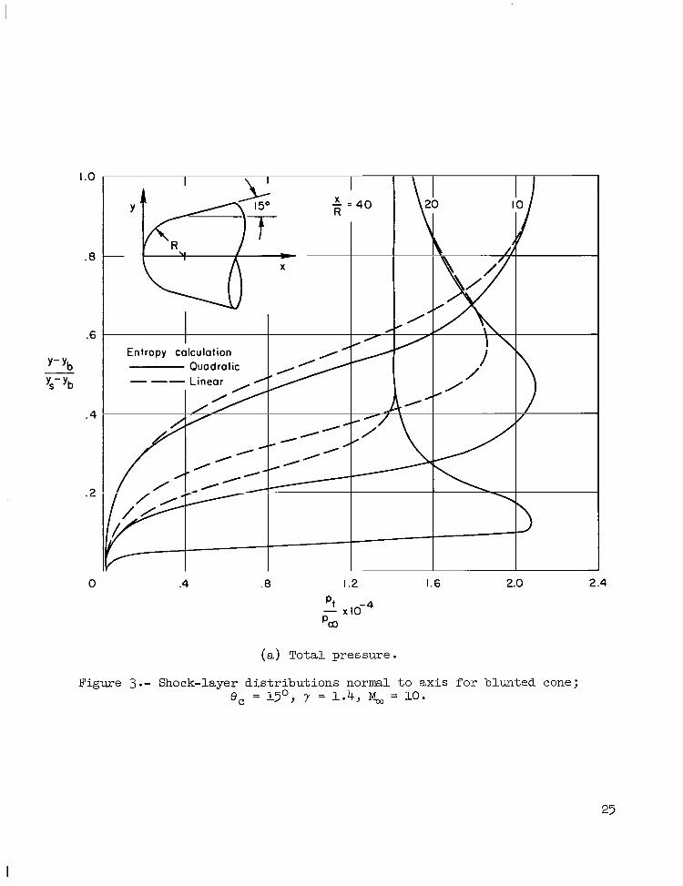
The flow f i e l d over a spherical ly blunted cone was calculated by the present method f o r surface-pressure d i s t r ibu t ion were unaffected by the entropy calculat ion. However, t he t o t a l pressure p ro f i l e s i n the shock layer a re s ign i f i can t ly d i f f e ren t as shown i n f igure 3 (a ) . (The ordinate i s the distance from the surface normalized by the t o t a l distance t o the shock.) associated with the overexpansion of t h e shock wave which occurs near x/R = 10. hence, the t o t a l pressure i n the shock layer has the maximum value of 2.1X104Xp, on the streamline passing through t h i s point . s ta t ion , t he t o t a l pressure on t h i s streamline must have the same value. The l i n e a r entropy interpolat ion smooths the t o t a l pressure d i s t r ibu t ion and erroneously reduces t h i s mximm value. x/R = 40, the entropy layer becomes so t h i n t h a t even quadratic interpolat ion i s not accurate near the body. because the inviscid entropy layer would have been absorbed within the

y = 1.4 and M, = 10. Both the shock-wave shape and

The differences a re

The entropy r i s e across the shock wave is a minimum there, and,

A t every downstream

Past

This deficiency i s usually unimportant from a p rac t i ca l standpoint

boundary layer . \

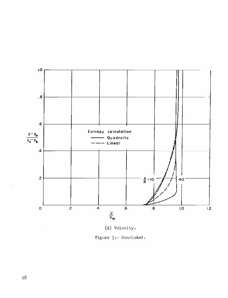
The s t a t i c pressure p ro f i l e s are not a f fec ted by the entropy calculat ion as shown i n f igure 3 (b ) . e f f ec t on the densi ty and ve loc i ty p ro f i l e s shown i n f igures 3(c) and 3 (d ) . The result i s t h a t t he mass-flow balance between the shock layer and the f r ee stream deter iora tes with distance as shown i n f igure 4. e r ro r i n the mass-flow balance is 9 percent with l i n e a r interpolat ion and negl igible w i t h quadratic interpolat ion.

However, the entropy calculat ion has a s igni f icant

A t x/R = 25, the

12

Similar comparisons have been made f o r a hemisphere cylinder f o r which the entropy gradients a r e not as la rge . Linear interpolat ion f o r the entropy yielded sa t i s fac tory r e s u l t s f o r the shock-wave shape, surface-pressure d is - t r ibu t ion , shock-layer prof i les , and mass-flow balance. These r e s u l t s cor- roborate the findings of reference 5 where l i n e a r interpolat ion f o r t he entropy was used, and checks of the mass-flow balance showed sa t i s f ac to ry agreement. These examples show t h a t f o r most bodies l i n e a r interpolat ion f o r t he entropy i s adequate f o r obtaining shock-wave shape and s ta t ic-pressure d is t r ibu t ion , but it may cause serious e r ro r s i n the other flow-field proper- t i e s i n regions with la rge entropy gradients . Since quadratic interpolat ion does not require an appreciable increase in the computing time, it is used exclusively i n the present method.

Comparison of Results From Present Method With Chushkin and Shulishnina

It is of i n t e re s t t o compare results from the present method with other calculat ions. Flow-field calculations by the method of charac te r i s t ics f o r blunted cones by Chushkin and Shulishnina ( r e f . 6) were recent ly brought t o our a t ten t ion . These calculat ions d i f f e r from the present method i n t h a t the subsonic-transonic solution was tha t obtained by Belotserkovskii ( r e f . 4) using the method of in tegra l r e l a t ions . I n addition, some differences are t o be expected in the computational procedure f o r t he method of charac te r i s t ics . Solutions were obtained f o r spherical ly blunted cones with half angles ranging from 0' t o 40° and fo r y = 1 . 4 and & = 4, 6, and 10. d i s t r ibu t ions i n the nose region from reference 6 and the present method are i n good agreement as shown i n f igure 5 . Although not shown i n the f igure, t h i s good agreement extends downstream u n t i l t he sharp-cone values a re reached.

The surface-pressure

Comparisons of pressure d is t r ibu t ions over cylinders w i t h e l l i p so ida l noses a re shown i n f igure 6 f o r y = 1.4 and For the slender or pro- l a t e e l l ipso id , the calculations proceeded smoothly, and the r e su l t s f r o m the present method show good agreement with the r e s u l t s of reference 6. For t he blunt or oblate e l l ipso id , the blunt-body solution used i n the present method i s i n e r ror i n the transonic region. However, the method of charac te r i s t ics solut ion quickly corrects t h i s e r ror , a t l e a s t , as f a r as the surface pressure i s concerned.

= 6.

Comparison With Experiment fo r a Body With Corners

As an i l l u s t r a t i o n of the embedded shock and expansion fan calculations, the flow over a blunt cone-cylinder-flare body w a s calculated f o r perfect a i r a t a Mach nmiber of 4.10. The r e s u l t s of the shock shapes obtained from t h i s calculat ion are shown i n f igure 7, and the surface pressures are shown i n f igure 8. ence 18. experiment and theory f o r the ellibedded shock on the f l a r e . a l so found for the experimental and calculated pressure d is t r ibu t ions i n f igure 8. tance along the f l a r e . This pressure var ia t ion i s caused by the increase of

Also shown i n these f igures a r e experimental r e s u l t s from refer - O f par t icu lar i n t e r e s t i n f igure 7 is the good agreement between

Good agreement is

Note t h a t the calculat ion predicts an increasing pressure with dis-

upstream dynamic pressure with distance from the corner, t h a t is, t he e f f ec t of the nonuniform upstream conditions created by the strong bow shock ( c f . ref . 9 ) .

Example of Solution fo r G a s Mixtures i n Thermodynamic Equilibrium

Flow-field solutions f o r gases i n thermodynamic equilibrium present no inherent d i f f i c u l t y as ide from an increase i n computing time required t o calculate the thermodynamic propert ies . However, the l imited accuracy of the r e a l gas propert ies obtained from the curve f i t s coupled with the d i f fe ren t calculat ion methods used i n the blunt body and method of charac te r i s t ics programs m y r e s u l t i n an incompatibil i ty along the input l i n e . For example, i n the blunt-body program the enthalpy i s determined with pressure and densi ty as inputs, whereas i n the method of charac te r i s t ics program the enthalpy i s determined with pressure and entropy as inputs . In regions where the curve f i t s a re poor, pa r t i cu la r ly near the limits of the tab les , the two values fo r enthalpy may be subs tan t ia l ly d i f f e ren t and may cause d i f f i c u l t i e s .

A s examples of flow-field calculations f o r r e a l gases, the pressure d is - t r i bu t ion on the blunt cone-cylinder-flare body studied in the preceding example i s shown i n f igure 9 f o r a i r and f o r a mixture of nitrogen and carbon dioxide. No unusual e f f ec t s a re noted compared with the e a r l i e r perfect gas r e s u l t s .

CONCLUDING REMARKS

The Ames computer programs f o r calculat ing the complete subsonic- supersonic flow f i e l d around blunt-nosed bodies a t zero angle of a t t ack were described. and flow charts f o r the main programs were presented. The flow charts should be helpful i n diagnosing d i f f i c u l t i e s o r making minor modifications fo r spec i f ic appl icat ions.

The more complex portions of the programs were explained i n d e t a i l ,

A number of example calculations were presented t o i l l u s t r a t e the appl i - c a b i l i t y and accuracy of the programs. r a t i c ra ther than the usual l i n e a r interpolat ion f o r entropy improved the accuracy of the method of charac te r i s t ics program. The improvement showed up especial ly i n the t o t a l pressure near the surface of blunt cones, where large entropy gradients develop, and i n the integrated mass flow across the shock layer f o r such bodies. Surface-pressure d is t r ibu t ions on blunted cones are i n agreement with published numerical r e s u l t s obtained by somewhat d i f fe ren t methods. Surface pressures and shock shapes, including the embedded shock, f o r a blunted cone-cylinder-flare, show good agreement with experiment.

It was shown tha t the use of a quad-

. -

Finally, t o i l l u s t r a t e app l i cab i l i t y t o flows of r e a l gases i n thermodynamic equilibrium, surface pressures on a f l a red body were presented for f l i g h t i n air and in a C02-N2 mixture.

Ames Research Center National Aeronautics and Space Administration

Moffett Field, C a l i f . , June 8, 1963

1. Van Dyke, Milton D.: The Supersonic Blunt-Body Problem - Review and Extension. J. Aerospace Sci., vol. 23, no. 8, Aug. 1958, pp. 485-496.

2. Batchelder, R. A.: An Inverse Method for Inviscid Ideal Gas Flow Fields Behind Analytic Shock Shapes. Douglas Aircraft Co., Inc., July 1963.

SM-42388, Missile and Space Systems Div.,

3. Lomax, Harvard; and Inouye, Mamoru: Numerical Analysis of Flow Properties About Blunt Bodies Moving at Supersonic Speeds in an Equilibrium Gas. NASA TR R-204, 1964.

4. Belotserkovskii, 0. M.: The Calculation of Flow Over Axisymmetric Bodies With a Detached Shock Wave. Computation Center, Acad. Sci., Moscow, USSR, 1961. AVCO Corp., 1962.

Translated: and edited by J. F. Springfield, RAD-TM-62-64,

5. Inouye, Mamoru; and Lomax, Harvard: Comparison of Experimental and Numerical Results for the Flow of a Perfect Gas About Blunt-Nosed Bodies. NASA TN D-1426, 1962.

6. Chushkin, P. I.; and Shulishnina, N. P.: Tables of Supersonic Flow About Blunted Cones. Computation Center Monograph, Acad. Sci., Moscow, USSR, 1961. Translated and edited by J. F. Springfield, RAD-TM-62-63, AVCO Corp., 1962.

7. Eastman, D. W.; and Radke, L. P.: Effect of Nose Bluntness on the Flow AIAA J., vol. 1, no. 10, Oct. 1963, Around a Typical Ballistic Shape.

pp . 2401-2402. 8. Palermo, D. A.: Equations for the Hypersonic Flow Field of the Polaris

Re-Entry Body. Aircraft Corp., Oct. 1960.

LMSD-480934, Lockheed Missiles and Space Div., Lockheed

9. Seiff, A.: Secondary Flow Fields Embedded in Hypersonic Shock Layers. NASA TN D-1304, 1962.

10. Jorgensen, Leland H.; and Graham, Lawrence A.: Predicted and Measured Aerodynamic Characteristics for Two Types of Atmosphere-Entry Vehicles. NASA TM X-1103, 1963.

11. Hayes, Wallace D.; and Probstein, Ronald F.: Hypersonic Flow Theory. Academic Press, New York, 1959.

12. Marrone, Paul V.: Inviscid, Nonequilibrium Flow Behind Bow and Normal Shock Waves, Part I. General Analysis and Numerical Examples. CAL Rep. w-1626~-12 (I), May 1963.

13. Bailey, Harry E .: Equilibrium Thermodynamic Properties of Carbon Dioxide. NASA SP-3014, 1965.

16

14. Walsh, J. L.; Ahlberg, J. H.; and Nilson, E. N.: Best Approximation Properties of the Spline Fit. J. Math. Mech., vol . 11, no. 2, March 1962, pp . 225-234.

15. Hilsenrath, Joseph, et al.: Tables of Thermal Properties of Gases.. . Cir . 564, U.S. National Bureau of Standards, Nov. 1, 1955.

16. Ferri, Antonio: The Method of Characteristics, Section G. Supersonic Flows With Shock Waves, Section H. General Theory of High Speed Aerodynamics, William R. Sears, ed., Princeton University Press, Princeton, New Jersey, 1954, pp. 583-747.

17. Powers, S. A.; and O'Neill, J. B.: Determination of Hypersonic Flow Fields by the Method of Characteristics. AUlA J., vol. 1, no. 7, July 1963, pp . 1693-1694.

18. Inouye, Mamoru; and Sisk, John B.: Wind-Tunnel Measurements at Mach Numbers F r o m 3 to 5 of Pressure and Turbulent Heat Transfer on a Blunt Cone-Cylinder With Flared Afterbody. NASA TM X-654, 1962.

TABU 1.- GAS MIXTURES ON AMES REAL-GAS TAPE

Composition by . volume i n percent

A i r : 78.2 N2, 21.8 02

F i l e number

2

1 Nitrogen 1 Carbon dioxide

' TABLE 11.- LIST OF SUBROUTINES

BLUNT-BODY PROGRAM

1 2

3 4

5 6

7

8

9

10

11 12

1 3

1 4 15

16 17

18

19

20

2 1 22

Subroutine name and I D no.

( i f any)

E X E C ~ ( T H O ~ O ~ ) ~ n c 2 ( ~ 0 7 0 2 1

OUT ( ~ ~ 0 7 0 4 ) SHOCK( ~ ~ 0 7 0 5 )

~ ~ ~ r v s ( ~ ~ 0 7 0 6 )

FIELDS ( THO707 )

BODYS(TH0709)

FIELDP ( ~ ~ 0 7 1 1 )

BODYSl(TH0712) FHIPSI (THO713)

TERP3 (TH0714)

SONIC (TH0715) 0 ~ ~ 7 ( ~ ~ 0 7 1 6 )

DERIVT (TH0717)

FIELDX( ~ ~ 0 7 1 8 )

POLY^ ( T H O ~ O )

LES2N ( THO72 3 )

SMOOTH(THO724)

D E R I V l (TH0725)

DIFFOR( THO733 )

Primary ca l l ing rout ine

MAIN MAIN

MAIN

BODYS

MAIN

STEP

EXEC2

BODYS

BODYS STEP SHOCK FIELDS

BODYS MAIN

BODYS

BODYS

BODYSl ERIVT

OUT

Subroutine function

Reads input cards Reads shock-shape parameters and calcu- l a t e s shock shape and slope Outputs free-stream conditions and f i e l d data a f t e r each s tep Calculates flow propert ies behind shock wave

Calculates der ivat ives i n s d i rec t ion

Calculates coef f ic ien ts f o r l i n e on which output data i s desired Predicts and corrects t he flow variables f o r the following s tep Calculates body loca t ion and f l o w propert ies Evaluates polynomial and f irst two deriv. a t ives for given value of argument Interpolates f i e l d data t o f ind proper- t i e s on output l i n e Smooths body coordinates Calculates s t r e a m function

Interpolates using +point Lagrange method

Locates sonic l i n e Outputs data f o r body and along output l i n e Different ia tes numerically t o obtain der ivat ives i n t d i rec t ion Stores s t a r t i n g data for the method of charac te r i s t ics on tape Evaluates coef f ic ien ts fo r second degree polynomial passing through three given points Evaluates coef f ic ien ts for least-squares f i t s t r a igh t l i n e Smooths data by f i l t e r i n g out high f re - quency osc i l l a t ions

Calculates der ivat ive using 5 points

Calculates four th differences ~. ~ - - . -~ L -

23

24

25

26

Subroutine name and I D no.

( i f any)

ENQZR ( THO737

RGAS

SERCH

LOCATE

TABLE 11.- LIST OF SE3ROUTINES

BLUNT-BODY PROGRAM - Concluded

Primary ca l l ing routine

BODYSl

EXEC1 SHOCK DERNS BODYS FPELDP OUT7 RGAS

. - _. -

Subroutine function .. -

Obtains running in tegra l of equally- spaced data

Calculates thermodynamic properties

Searches f o r coeff ic ients f o r real-gas propert ies Locates tape a t specified f i l e pos i t ion

-~ ._ ~

20

.. ..

1

2 3

4

5

6

7

8

9

10

11

12

1 3

14

15

16

17 18 1 9

20 21

lubrout ine namc and I D no.

( i f any)

EXEC

MID

BOT ( ~ ~ 2 4 2 3 )

ESHOCK

GSHOCK

C SHOCK

EXPAN

SHOCK

RGAS

ROOTB ( TE42 6)

CON( ~ ~ 2 4 1 1 )

DATA(TE425)

TPRES(TH2429)

ISENC ESPACl(TH24-09 ESPACE (TH2412

NTEFG? TERP3(W405)

TABLE 111.- LIST OF SUBROUTINES

METHOD OF CHARACTERISTICS PROGRAM

Primary ca l l i ng rout ine

MAIN

MAIN MAIN

MAIN

MAIN

MAIN

ESHOCK

ESHOCK

ESHOCK

GSHOCK C SHOCK EDAN

BOT

M I D

EXEC

EXEC ESPACl

Subroutine function

Reads input cards, reads input tapes, i n i t i a l i z e s var iables Reads addi t ional input data Locates new 'bow shock point and calcu- l a t e s the new shock angle Locates new mesh points and i t e r a t e s f o r solut ion of equation (10) Locates new body point and i t e r a t e s f o r body data Keeps t r ack of embedded shocks and ad jus ts storage loca t ions i n P array; interpolates f o r conditions on the body upstream of a corner Locates general embedded shock point and calculates new shock angle Calculates shock angle a t a corner, and a t the f i rs t mesh point away from the corner Calculates addi t iona l points f o r an expansion corner, and ad jus ts storage locat ions i n P a r r a y Calculates the shock jump conditions given the shock angle and upstream conditions Calculates Prandtl-Meyer flow given the expansion angle and upstream conditions Calculates gas properties; reads RGAS tape Locates in te rsec t ion of right-running charac te r i s t ic with the body Calculates averages of the coeff ic ient : of equation (10) Reads s t a r t i n g flow-field da ta i f specif ied on cards Calculates t o t a l pressure Calculates one-dimensional isentropic flow between given v e l o c i t i e s Prepares data f o r equal spacing Equally spaces da ta with respect t o a given var iable Interpolat ing rout ine Interpolat ing rout ine

~~ ~ ~~

2 1

22 23 24 25 26

27

28

29

30

31 32

33

TABLE 111.- LIST OF SUBROUTINES

METHOD OF CHARACTEFUSTICS PROGRAM - Concluded

Subroutine name and I D no. (if any)

TERP4 ( ~ ~ 2 4 0 6 ) POLY3 (TH2.408) HEM ENQ55R (THO737 SHOCKP ( ~ ~ 4 8 7

BODYP (~H2.488 )

SEARCH ( ~ ~ 2 4 8 9

SERCHl(TW416)

PRINTF ( TH2.48 6 )

SERCH PLOTS

LOCATE

Primary ca l l ing rout ine

MAIN

MAIN

MAIN

BODYP

MAIN

RGAS MAIN

Subroutine function

Interpolat ing routines

Integration routine Interpolates f o r data a t prescribed points along the bow shock Interpolates f o r data a t prescribed points along the body Interpolates f o r data along a charac- t e r i s t i c l i n e Calculates equations of body normal probe l i n e s Stores data along body or axis normals; s tores last probe on tape Scans RGAS t ab l e f o r per t inent data Dummy subroutine - can be used t o write a p lo t tape using data i n P a r r ay Locates specif ied f i l e posi t ions on data storage tape

22

Start

Read input Yes

Perturb shock shape shock

t

t

Calculate

behind shock PIP, u,

Output shock data and

set i= I

1 --------- Calculate l - a+ 'dt' dt' x ( t ) ap ap au a

t I Calculate

I I I I I I I I I I I I

I Output body and probe line data

I Store probe

line data

I Interpolate field data

along probe

1 No

I Compare body

points with desired shape

1 I No Predict and correct

P, P I u, (v/t) for ( i t I) th step

i = i + I

4 Output data Extra polo te for ( i+ l ) th for

step body data

Figure 1.- Flow chart f o r blunt-body program.

23

I I I I I I I I I I I I I I I I I I I I I I I I I I I I I I I

Start

- - - i i bow shock

I

Calculate

~ ~ e .

expan:in fan) rl along probe

Figure 2.- Flow chart for characteristics program.

24

I .o

.8

.6

Y- Yb

's- 'b

. 4

.2

0 .4 .8 I .2 1.6 2.0 2.4

(a) Total pressure.

Figure 3.- Shock-layer d i s t r ibu t ions normal t o ax i s f o r blunted cone; e, = i 5 O , 7 = 1.4, r/6, = i o .

25

1.0

. 8

. 6

-4

. 2

0 2 4 6 0 IO P

PaD -

(b) S t a t i c pressure.

I

12

Figure 3 .- Continued.

26

1.0

. 0

.6

Y - Y b

ys-y b

.4

.2

0

- 1 1 Entropy CalCUlatlOn

- - - Linear

I I

Quadratic

I 2 3 4 5 6 P

Pa0 -

( c ) Density.

Figure 3. - Continued .

Entropy c a l c u l a t i o n

Q u a d r a t i c --- Linear

0 .2 .4 .6 .0 V - v,

(d) Velocity.

Figure 3 .- Concluded.

1.0 1.2

28

Quadrat i c inter p o la t ion n U

YS

12.nYPU dY

yb

VY; Pm"m .8

+-e -&--+-- Linear i n t e r p o l a t i o n

." 0 IO 20 30 40 50

Figure 4.- Effect of entropy calculation on mass flow balance f o r blunted cone; 8, = l5', y = 1.4, M, = 10.

Iu \o

- Present method 1 0 M e t h o d of r e f . 6

0 .2 .4 .6 .8 1.0 1.2 I .4

(a) M, = 4

Figure 5.- Surface-pressure d i s t r ibu t ion on blunted cone, y = 1.4 .

30

60

50

40

30

20

IO

- ' 8 PaY

6

5

4

3

2

I 0 .2

n v

Present method - 0 Method of re f .6

1 !

I l l

T- T I

.6 .a I .o 1.2 I .4 X - R

Figure 5 .- Continued.

'0 .2 .6

0

I I - Present method

Method of ref. 6

.8 1.0 I .2 1.4

( c ) M, = 10

Figure 3 . - Concluded.

60

50

40

30

20

10

- p 8 pco

6

5

4

3

2

I 0 .2

I Present method I - Bb

.4 .6 .8 1.0 1.2 1.4 X - b

Figure 6 .- Surface-pressure d i s t r ibu t ion on e l l i p s o i d cylinder; 7 = 1.4, M, = 6.

33

h

w c-

c

- I 0 I 2 3 I I I I I I I 4 5 6 7 a 9 IO I I 12 13

I I I

X - R

14

Figure 7.- Comparison of theore t ica l and experimental shock-wave shapes for a f la red body; y = 1.4, = 4.1.

W wl

40

20

I O

8

6

2

I .o .8

.6

0 2

Present met hod 0 Experiment, ref, 18 -

4 6 8

R X -

IO 12 14

Figure 8.- Comparison of theoret ical and experimental surface pressures for the f la red body of f igure 7; y = 1.4, = 4.1.

W cn 600

40 0

20 0

I O 0 80

60

20

I I

O 2 4 6 a X - R

I O 12 14

Figure 9.- Comparison of surface-pressure d is t r ibu t ions on f l a r ed body of f igure 7 f o r a i r and fo r a mixture composed of 31.2 percent Nz, 48.8 percent C02; V, = 6.10 km/sec, p, = 1.225 g/m3, p, = 101.2 N/m2.

t

“The aeronautical and >pare activities of the Uniled States shall be conducted so as i o conlribute . . . to the expatision of hitman Rtiowl- edge of phenomena in the atmosphere atid space. The Adtninisiratiotr shall provide for the widest practicable and appropriate dissemination of information concerning its actiuilies and the results thereof .”

-NATIONAL AERONAUTICS AND SPACE ACT OF 1958

NASA SCIENTIFIC A N D TECHNICAL PUBLICATIONS

TECHNICAL REPORTS: important, complete, and a lasting contribution to existing knowledge.

TECHNICAL NOTES: of importance as a contribution to existing knowledge.

TECHNICAL MEMORANDUMS: Information receiving limited distribution because of preliminary data, security classification, or other reasons.

CONTRACTOR REPORTS: Technical information generated in con- nection with a NASA contract or grant and released under NASA auspices.

TECHNICAL TRANSLATIONS: Information published in a foreign language considered to merit NASA distribution in English.

TECHNICAL REPRINTS: Information derived from NASA activities and initially published in the form of journal articles.

SPECIAL PUBLICATIONS: Information derived from or of value to NASA activities but not necessarily reporting the results .of individual NASA-programmed scientific efforts. Publications include conference proceedings, monographs, data compilations, handbooks, sourcebooks, and special bibliographies.

Scientific and technical information considered

Information less broad in scope but nevertheless

Details on the availability o f these publications may be obtained from:

SCIENTIFIC AND TECHNICAL INFORMATION DIVISION

N AT1 0 N A L A E R 0 N A UTI CS A N D SPACE A DM I N I STRATI 0 N

Washington, D.C. PO546

Documents

A description of numerical methods and computer programs ... · PDF filecomputer programs for two-dimensional and axisymmetric supersonic flow ... and axisymmetric supersonic flow