MET 112 Global Climate Change – Lecture 10

Recent Climate Change

Dr. Craig ClementsSan Jose State University

Outline Recent trends in temperature Recent trends in GHGs Time scales

(b) Additionally, the year by year (blue curve) and 50 year average (black curve) variations of the average surface temperature of the Northern Hemisphere for the past 1000 years have been

reconstructed from “proxy” data calibrated against thermometer data (see list of the main proxy data in the diagram). The 95% confidence range in the annual data is represented by the grey

region. These uncertainties increase in more distant times and are always much larger than in the instrumental record due to the use of relatively sparse proxy data. Nevertheless the rate and

duration of warming of the 20th century has been much greater than in any of the previous nine centuries. Similarly, it is likely7 that the 1990s have been the warmest decade and 1998 the

warmest year of the millennium.

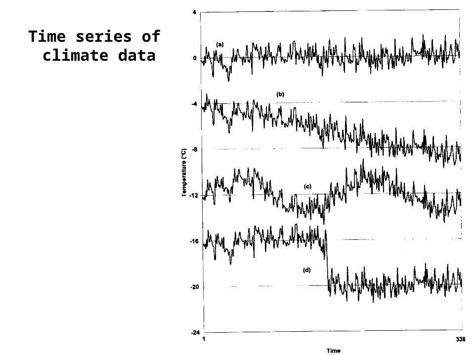
Time series of climate data

Time series of climate data

Examples of Temperature Change

Trends Periodic Oscillations Random Variations Jumps

Examples of Temperature Change

Draw the following:

1. Trend2. Oscillation3. Trend + Oscillation4. Random variations5. Random + trend6. Jump7. Random + jump

Trend

100806040200Time

Tem

pera

ture

This graphs represents

1. Trend

2. Oscillation

3. Trend+Oscillation

4. Random variation

5. Random+Trend

6. Jump

7. Random+Jump

100806040200Time

Tem

pera

ture

This graphs represents

1. Trend

2. Oscillation

3. Trend+Oscillation

4. Random variation

5. Random+Trend

6. Jump

7. Random+Jump

100806040200Time

Tem

per

atu

re

This graphs represents

1. Trend

2. Oscillation

3. Trend+Oscillation

4. Random variation

5. Random+Trend

6. Jump

7. Random+Jump

100806040200Time

Tem

per

atu

re

This graphs represents

1. Trend

2. Oscillation

3. Trend+Oscillation

4. Random variation

5. Random+Trend

6. Jump

7. Random+Jump

100806040200Time

Tem

per

atu

re

This graphs represents

1. Trend

2. Oscillation

3. Trend+Oscillation

4. Random variation

5. Random+Trend

6. Jump

7. Random+Jump

100806040200Time

Tem

pe

ratu

re

This graphs represents

1. Trend

2. Oscillation

3. Trend+Oscillation

4. Random variation

5. Random+Trend

6. Jump

7. Random+Jump

100806040200Time

Tem

per

atu

re

Time Frames -- Examples Seconds to minutes – Small-Scale Turbulence Hours – Diurnal Cycle (Caused by Earth’s

Rotation) Hours to Days – Weather Systems Months – Seasonal Cycle (Caused by tilt of

axis) Years – El Niño Decades -- Pacific Decadal Oscillation Centuries – Warming during 20th Century

(Increase in greenhouse gases?) Tens of thousands of Years – Irregularities in

Earth’s motions Millions of Years – Geologic Processes

Cli

mat

e C

hang

e

Cli

mat

e “V

aria

bili

ty”

Latest global temperatures

…“Over the last 140 years, the best estimate is that the global average surface temperature has increased by

0.6 ± 0.2°C” (IPCC 2001)

So the temperature trend is: 0.6°C ± 0.2°C

What does this mean?

Temperature trend is between 0.8°C and 0.4°C

The Uncertainty (± 0.2°C ) is critical component to the observed trend

Current CO2: ~383 ppm

What Changed Around 1800?

Industrial Revolution– Increased burning of fossil fuels

Also, extensive changes in land use began– the clearing and removal of forests

Burning of Fossil Fuels

Fossil Fuels: Fuels obtained from the earth are part of the buried organic carbon “reservoir”– Examples: Coal, petroleum products,

natural gas The burning of fossil fuels is essentially

– A large acceleration of the oxidation of buried organic carbon

Land-Use Changes

Deforestation: – The intentional clearing of forests for

farmland and habitation This process is essentially an acceleration of

one part of the short-term carbon cycle: – the decay of dead vegetation

Also causes change in surface albedo (generally cooling)

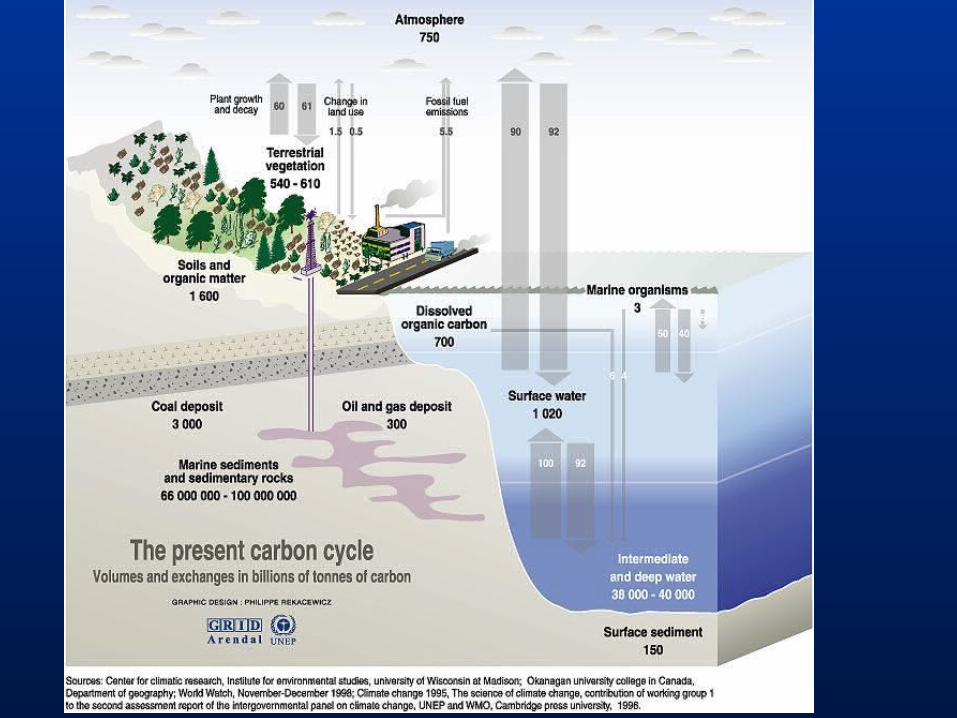
Natural Short-Term Carbon Cycle – Quantitative

Atmosphere

Biosphere Ocean

Carbon Content: 750 Pg*

1 Pg = 1015 g

Carbon Content: 2000 Pg

Carbon Content: 38, 000 Pg

Carbon Flux: ~ 120 Pg/year

Carbon Flux: ~ 90 Pg/year

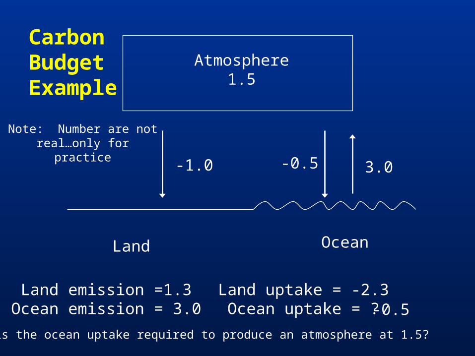
CarbonBudgetExample

Atmosphere1.5

OceanLand

Land emission =1.3Ocean emission = 3.0

Land uptake = -2.3Ocean uptake = ?

Note: Number are not real…only for practice

Positive values refer to carbon going into the

atmosphere

What is the ocean uptake required to produce an atmosphere at 1.5?

The ocean update is:

1.5

-1.5

-0.5 0 1 -1

0%

8%

0%3%

0%

89%1. +1.5

2. -1.5

3. -0.5

4. 0

5. 1.0

6. -1.0

CarbonBudgetExample

Atmosphere1.5

OceanLand

Land emission =1.3Ocean emission = 3.0

Land uptake = -2.3Ocean uptake = ? -0.5

Note: Number are not real…only for practice

What is the ocean uptake required to produce an atmosphere at 1.5?

-1.0 3.0-0.5

CarbonBudgetExample Notes…

Land/atmosphere Flux = Land emission + Land uptake

Ocean/atmosphere Flux = Ocean emission + ocean uptake

Carbon Budget Changes

Units in Peta-grams (x1015) of Carbon per year (PgC/yr) Atmosphere increase 3.3 ± 0.1

– Observations Emissions (fossil fuel, cement) 5.4 ± 0.3

– Estimates from industry Ocean-atmosphere flux -1.9 ± 0.6

– Estimates from models/obs

Final component is Land/atmosphere flux: What is the land/atmosphere flux?

CarbonBudgets

Atmosphere

OceanLandFossil fuel

burning

5.4 PgC -1.9 PgC

3.3 PgC

Land/atmosphere flux Ocean/atmosphere flux

Please make your selection...

4 -4 3.5

-3.5 0.

2-0

.2

0% 0%

95%

5%0%0%

1. +4.0

2. -4.0

3. +3.5

4. -3.5

5. +0.2

6. -0.2

CarbonBudgets

Atmosphere

OceanLandFossil fuel

burning

5.4 PgC -1.9 PgC-0.2 PgC

3.3 PgC

Land/atmosphere flux Ocean/atmosphere flux

Carbon Budget (II)

Land atmosphere flux partitioned as follows 

Land use change– From observations

-0.2±0.7

1.7

Land atmosphere flux– Must be to balance budget

Residual terrestrial sink Calculated to balance land/atmosphere flux

CarbonBudgets

Atmosphere3.3 PgC

OceanLandFossil fuel

burning

5.4 PgC -1.9 PgC-0.2 PgC

Land use change1.7 PgC

So, now considering the land use change, what is the new Land/atmosphere flux?

Land/atmosphere flux

What is the residual land sink?

1. -1.9

2. -1.7

3. +0.2

4. 1.5

CarbonBudgets

Atmosphere3.3 PgC

OceanLandFossil fuel

burning

5.4 PgC -1.9 PgC-0.2 PgC

Land use change1.7 PgC

-1.9

So, now considering the land use change, what is the new Land/atmosphere flux?

Land/atmosphere flux

Carbon Budget (II)

Land atmosphere flux partitioned as follows 

Land use change– From observations

-0.2±0.7

1.7

-1.9

Land atmosphere flux– Must be to balance budget

Residual terrestrial sink Calculated to balance land/atmosphere flux

Human Perturbation of the Carbon Cycle

Carbon Budget (III)

There are significant uncertainties related to these budget terms.

Main questions are related to:

– Can biosphere/ocean take up more atmospheric CO2?– What are the carbon fluxes over different types of ecosystems

Tropical forests, Temperate forests, Boreal forests, Tropical savannas & grasslands, Temperate grasslands & shrub lands, deserts and semi deserts, Tundra, Croplands, Wetlands

– What happens if the land/ocean get ‘saturated’ with carbon?

Video – Global Warming – signs and the science

Explain the concept of ‘ancient sunlight’ and how it relates to the carbon cycle.

Carbon Budget (III)

Greenhouse Gases

Carbon Dioxide Methane Nitrous Oxide CFCs (Chlorofluorocarbons) Others

Methane

Anthropogenic Methane Sources

Leakage from natural gas pipelines and coal mines

Emissions from cattle – Flatulence…gas

Emissions from rice paddies

Nitrous Oxide

Anthropogenic Sources of Nitrous Oxide

Agriculture

CFCs

CFC-11

CFC-12

Sources of CFCs

Leakage from old air conditioners and refrigerators

Production of CFCs was banned in 1987 because of stratospheric ozone destruction– CFC concentrations appear to now be

decreasing – There are no natural sources of CFCs

Lecture on ozone depletion to follow later in semester…

Latest global temperatures

Activity

1. Describe the 120 year temperature records in terms of the seven above described types of variations (trend, trend+oscillation etc.) by breaking up the time series into periods (i.e. from 1930-1950, oscillation + positive trend, from 1950-1970, negative trend)

2. Based on the past 120 years of globally averaged temperatures:a. What trend would you assign to this period. (i.e.

0.3°C over 120 years)b. If you were to break up the data into time sections

provide trends over the following time periods i) 1880-1920; b) 1920-1940 and c) 1970-2000

How would you describe the last 30 years of temperature

Ran

dom

Osc

illat

ion

Osc

illat

ion+t

rend

Osc

illat

ion+j

ump

Ran

dom

+jum

p

Tre

nd

0% 0% 0%0%0%0%

1. Random

2. Oscillation

3. Oscillation+trend

4. Oscillation+jump

5. Random+jump

6. Trend

0 of 250

What is the approximate temp trend over the last 30 years?

0 of 250 0

.6C/3

0 ye

ars

1.0

C/30

year

s

.1C/3

0 ye

ars

0.2

C/30

year

s

0% 0%0%0%

1. 0.6C/30 years

2. 1.0C/30 years

3. .1C/30 years

4. 0.2C/30 years

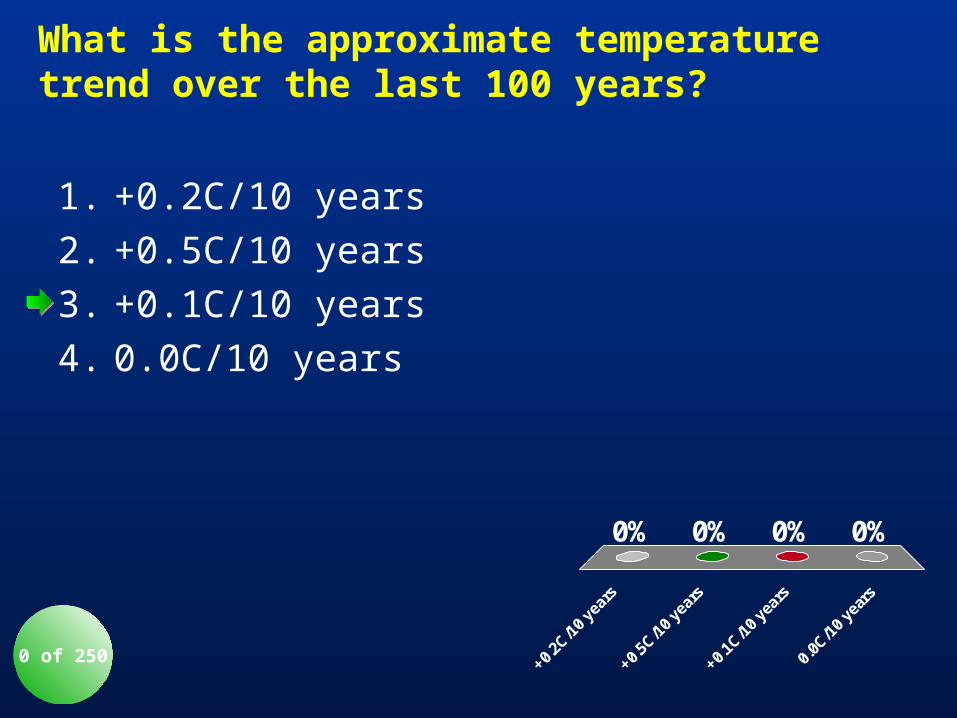
What is the approximate temperature trend over the last 100 years?

+0.

2C/1

0 ye

ars

+0.

5C/1

0 ye

ars

+0.

1C/1

0 ye

ars

0.0

C/10

year

s

0% 0%0%0%

1. +0.2C/10 years

2. +0.5C/10 years

3. +0.1C/10 years

4. 0.0C/10 years

0 of 250

Temperature over the last 10 years

Comparison of 1998 with 2005

The Land and Oceans have both warmed

Precipitation patterns have changed

Activity 11 Question

Explain how humans may affect precipitation in a city.