Medium-Scale Experiments on Stabilizing Riser-Slug Flow

156 December 2009 SPE Projects, Facilities & Construction

Medium-Scale Experiments on Stabilizing Riser-Slug Flow

Heidi Sivertsen,* Vidar Alstad,** SPE, and Sigurd Skogestad, Norwegian University of Science and Technology

* Now with Statoil, Stjørdal, Norway.

** Statoil Research Centre, Porsgrunn, Norway.

Copyright © 2009 Society of Petroleum Engineers

Original SPE manuscript received for review 24 July 2008. Revised manuscript received for review 11 May 2009. Paper (SPE 120040) peer approved 23 May 2009.

SummaryThis is the second of two papers describing control experiments on a medium-scale slug rig. The first paper (Sivertsen et al. 2009) describes experiments performed on a small-scale laboratory rig built at the Norwegian University of Science and Technology (NTNU) Department of Chemical Engineering. These experiments showed that, despite noisy measurements, it is possible, with feed-back control, to “stabilize the flow” (i.e., to achieve reasonably smooth flow in the normally riser-induced severe slug-flow region) using only topside measurements. The question to be answered is whether these results also apply for larger riser systems.

In the present paper, we look at some results obtained from a 10-m-high, 3-in.-diameter medium-scale test rig located at the Statoil Research Centre in Porsgrunn, Norway. Several cascade control structures are tested and compared, both with each other and with the results obtained from the small-scale NTNU loop. The rig was also modeled and analyzed using a simple three-state dynamic model.

The new experiments were successful and confirm the results of Sivertsen et al. (2009) from the small-scale rig. The valve opening with nonslug flow operation could be increased from approximately 12% with no control to almost 24% with control using topside measurements only. This makes it possible to pro-duce with a larger production rate and increase the total recovery from the producing oil field. The valve opening with control could be further increased to approximately 28% using measurements from the bottom of the riser, but such measurements may not be available in many cases.

BackgroundThe behavior of multiphase flow in pipelines is of great concern in the offshore oil and gas industry, and much time and effort have been spent studying this phenomenon. The reason for this is that, by making relatively small changes in operating conditions, it is possible to change the flow behavior in the pipelines dramatically. This has a huge influence on important factors such as productivity, maintenance, and safety.

Active control makes it possible to avoid the slug-flow regime with conditions where slug flow is predicted. This way, it is possible to operate with the same average flow rates as before but without the large oscillations in flow rates and pressure. The advantages with using active control are large: It is much cheaper than implementing new equipment, and it removes the slug flow altogether, thereby removing the strain on the system. This way, savings can be realized in maintenance costs. Also, it is possible to produce larger flow rates than those that would be possible by choking the topside valve manually.

Several experiments were performed to test control configura-tions similar to those tested on the NTNU small-scale laboratory rig. This was done to investigate whether different scales have an effect on the quality of the control structures. Having results from a larger-scale rig could give an indication on whether the small-

scale NTNU laboratory rig really was suitable as a tool for finding good control solutions to be used in larger-scale facilities, such as an offshore production system.

The question was whether active control could also be used to stabilize the flow for the medium-scale laboratory rig. In particu-lar, it was interesting to see whether only topside measurements could be used to stabilize the flow, as was done on the small-scale laboratory rig described in Sivertsen et al. (2009).

Experimental SetupEarlier studies on using only topside measurements are found in Godhavn et al. (2005), where experiments were performed on a larger rig and the flow was controlled using combinations of pressure and density measurements. The results, however, were not compared with what is obtainable from using subsea measure-ments in the control structure. Experiments similar to the ones described in the present paper were performed earlier on a small-scale laboratory rig. These experiments are described in Sivertsen et al. (2009).

The medium-scale multiphase-flow-control rig at the Statoil Research Centre in Porsgrunn is built to simulate multiphase flow in an offshore well/pipeline and production unit. The facility is ideal for development and testing of new control solutions for antislug and separator control under realistic conditions. Fig. 1 shows a photograph of the facility.

During the experiments, the flow consisted of water and air. The pipe diameter is 3 in. (7.6 cm), and the height of the riser is approximately 10 m. The inflow of gas and water was pressure-dependent. The water-inlet rate during the experiments was from 7 to 8 m3/h, while the air-inflow rate fluctuated between 8 and 11 m3/h. Slugging occurred for valve openings larger than approxi-mately 12%. Fig. 2 shows a schematic overview of the layout and available instrumentation.

The loop includes an approximately 4-m-long section where gas, oil, and water are introduced through different inlets. This “well section” consists of annulus and tubing, a 15.2-cm-diameter outer pipe and a 7.6-cm-diameter inner tubing with perforations.

The pipe section consists partly of flexible tubing, hence it is possibly to vary the geometry of the piping. This way, the incli-nation of the riser and other parts of the pipe can be adjusted to achieve the desired geometry.

The pipeline geometry during the experiments was chosen to give terrain-induced slugging. A more-detailed schematic of the geometry used in the experiments is shown in Fig. 3. The numbers indicate the location of feeding inlets and important instrumentation.

The numbers 1, 2, and 3 indicate the air, water, and oil inlets, respectively. Downstream, this section of the pipeline is close to horizontal for approximately 10 m. An approximately 7-m, 35° inclined section then follows. A pressure measurement (P1) is located at the end of this section (4). The next 60-m section has a 1.8° declination, followed by an approximately 20-m horizon-tal section with a pressure and temperature measurement at the end (6). A 10-m-long vertical riser then follows a low point in the geometry (7). The low point contains a see-through section, which makes it possible to determine the flow regime in this sec-tion visually. At the top of the riser are a production choke (10) and separator (11). A pressure measurement (8) and a see-through section (9) are located half-way up the riser. Upstream of the pro-duction choke, pressure measurement (P2) is taken and a gamma densitometer is used.

skoge

Sticky Note

Misprint in figure captions for Figures 12, 13 and 14: "outer loop" and "inner loop" should be interchanged.

December 2009 SPE Projects, Facilities & Construction 157

Fig. 1—A birds-eye view perspective of the medium-scale riser rig at Statoil Research Centre in Porsgrunn.

Fig. 2—Schematic overview of the layout and available instrumentation.


The water and oil outlets from the separator are returned to a large 10-m3 buffer tank. The oil and water feed are pumped from this buffer tank back to the respective phase inlets in the well section by use of two displacement pumps. Before entering the well section, the feed-flow rate and density of each phase are measured.

Gas Feed. The compressed air is supplied from the local air supply net. The supplied air holds a pressure of approximately 7 bara. An automated control valve controls the feed-fl ow rate of compressed air to the well section. The operating range of the control valve is from 10 to 400 kg/h.

The mass flow and the density of the compressed air are mea-sured using a Coriolis-type mass flowmeter.

Water Feed. A displacement pump controls the feed-fl ow rate of water. The power is either set directly by the operator or given as output from a feedback controller using the volumetric fl ow rate as measurement. The pressure and single-phase-fl ow rates are measured downstream of the pumps, using a Coriolis-type mass fl owmeter for the water.

Separator. The three-phase separator located at the top of the riser has a volume of approximately 1.5 m3. A 53-cm-high weir plate separates the oil and water outlets. The separator is equipped with a pressure measurement and measurements of the oil and water levels. No oil was added to the fl ow during the experiments presented in this paper.

Control Choke Valve. The control choke valve is a vertically po-sitioned valve located at the top of the riser. The valve is equipped with a positioner, which returns the actual valve position to the control system.

Choke-Valve Characteristics. Several flow experiments had been performed in order to find the single- and two-phase (water/air) valve characteristics:

F C f zP

Q v

K z

= ( ) Δ( )

�. . . . . . . . . . . . . . . . . . . . . . . . . . . . . . . . . (1)

Cv is the valve constant and f(z) is the characteristics of the valve. �P is the pressure drop across the valve and � is the density of the fluid. For valve openings less than 50 and 60% for single-phase and two-phase flow, respectively, the characteristics were found to be close to linear. Thus, Eq. 1 can be written as

F C zP

Q v = Δ�

. . . . . . . . . . . . . . . . . . . . . . . . . . . . . . . . . . (2)

Values for FQ /Cv can be calculated from given values for valve opening z, measured pressure drop across the valve �P, and mea-sured density �.

Instrumentation. A number of automatic control valves are in-stalled. This includes the production choke valve; the valves con-trolling gas, water, and oil outlet from the separator; and the feed fl ow of air to the well section. These valves can be operated either in manual mode or in automatic mode where valve openings are given as output from proportional, integral, and derivative (PID) feedback controllers. The rig is controlled from a control room located close to the rig.

Controllability Analysis Modeling. In Sivertsen et al. (2009), it was shown how an analysis of a model describing a small-scale laboratory rig did reveal fun-damental control limitations, depending on which measurements were used for control. This was found using a simplifi ed model (Storkaas et al. 2003). One of the advantages of this simple model is that it is well-suited for controller design and analysis. It con-sists of three states: the holdup of gas in the feed section (mG1) and in the riser (mG2), and the holdup of liquid (mL). The model is illustrated in Fig. 4.

The same model was used to predict the behavior for the medium-scale laboratory rig used in this study. Using this model, the system was analyzed in the same way as in Sivertsen et al. (2009). Both open- and closed-loop simulations were performed.

After entering the geometrical and flow data for the laboratory rig, the model was tuned as described in Storkaas et al. (2003) to fit the open-loop behavior of the laboratory rig. The model data and tuning parameters are presented in Table 1. After inserting new system parameters and retuning the model, the open-loop data found using the model fit the experimental results quite well, as shown by the bifurcation plot in Fig. 5.

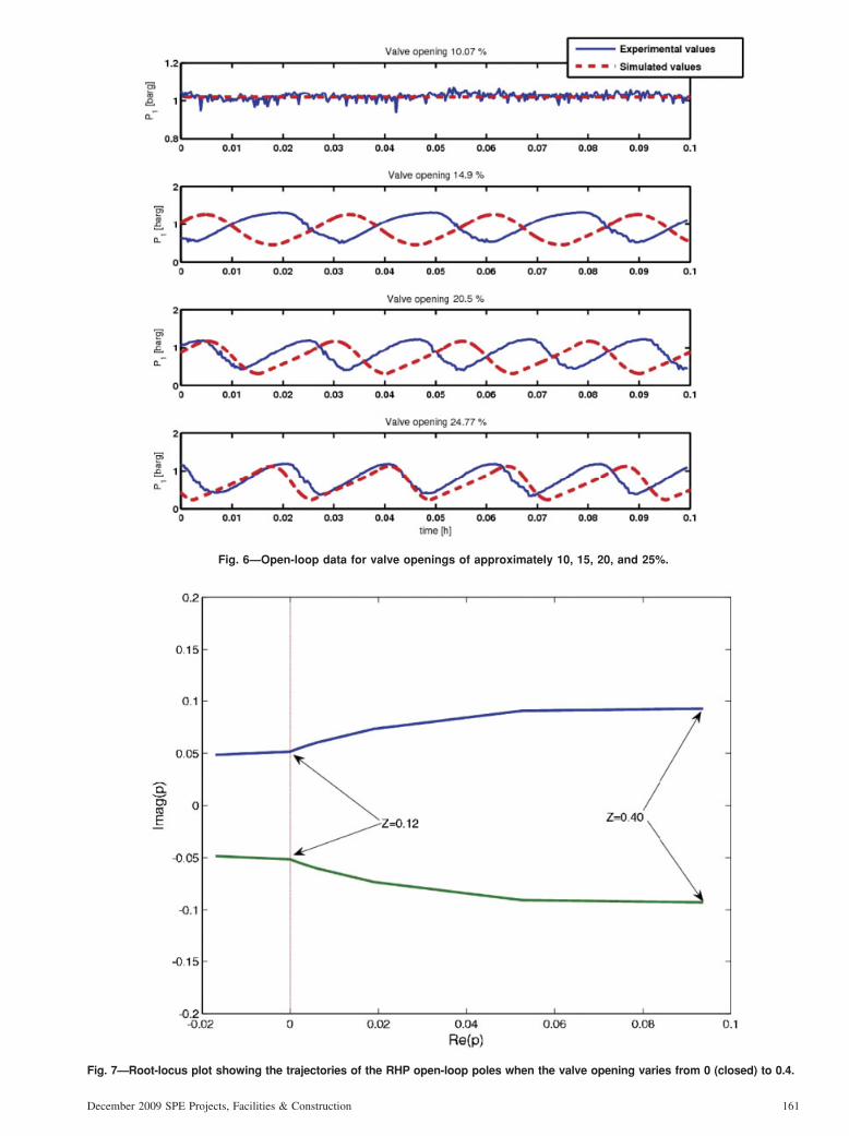
The bifurcation diagram gives information about the valve opening for which the flow becomes unstable and shows the amplitude of the pressure oscillations for the inlet and topside pressures (P1 and P2). The upper lines in the bifurcation plot show the maximum pressure at a particular valve opening, and the lower line shows the minimum pressure. The lines meet at the bifurca-tion point when the valve opening is approximately 12%. This is

Fig. 3—Schematic of the geometry of the riser system.


the point where transition to slug flow occurs naturally, and this is the highest valve opening that gives nonslug behavior in open-loop operation without control. The dotted line in the middle shows the unstable nonslug solution predicted by the model. This is the desired operating line with closed-loop operation.

The bifurcation plot was obtained by open-loop simulations of the system at different valve openings. Some of these results are plotted in Fig. 6 together with experimental results. The model fit the experimental data quite well, in terms of both amplitude and frequency of the oscillations. Note that a shift in time does not matter. The match between simulated and experimental results is especially good for a valve opening of 14.9%.

In Fig. 7, a root-locus diagram of the system is plotted. This shows how the poles, computed eigenvalues from the model, cross into the right half plane (RHP) of the imaginary plane as the valve opening reaches 12% from below. This confirms what was seen in the bifurcation diagram.

Analysis. The model can now be used to explore different measurement alternatives for controlling the flow. The following measurements were analyzed in this study: inlet pressure P1, pres-sure upstream of production choke P2, density �, mass-flow rate

FW, and volumetric flow rate FQ through the topside choke. Fig. 8 shows the different measurement candidates.

In Sivertsen et al. (2009), it was shown for the small scale laboratory rig how the RHP poles and zeros and their locations compared with each other in the imaginary plane had a large influ-ence on the controllability of the system. By scaling the system and calculating the sensitivity peaks, it is possible to get a picture of the challenges in terms of stabilizing the system.

The analysis is described in Appendix A. It shows that we might expect problems because of RHP pole/zero location when using a topside density measurement or pressure as single measurements for control. In addition, the analysis discovers that we might experience problems because of drift (low steady-state stationary gain) when using topside flow measurements. These are results similar to those found for the small-scale laboratory rig in Sivertsen et al. (2009).

Simulations. Closed-loop simulations were performed to inves-tigate the effect of the limitations found in the analysis. The measurements were used as single measurements in a feedback loop with a proportional-integral (PI) controller. Fig. 9 shows this control structure using the inlet pressure P1 as the measurement.

(a) Simplified representation of riser slugging

(b) Simplified representation of desired flow regime

Feed Pipeline

Choke Valve With opening Z

Choke Valve with opening Z

wmix,out

P0

L3

H2

H1

VL

mL

h1

h1>H1=>vG1=wG1=0

mG2 ,P2, VG2, ρG2, αLT

mG1 ,P1, VG1, ρG1

wmix,out

P0

L3

H2

H1VL

mL

h1

h1<H1

mG2 ,P2, VG2, ρG2, αLT

mG1 ,P1, VG1, ρG1

vG1, wG1

θ

θ

wL,inwG,in

wL,inwG,in

Fig. 4—Storkaas’ pipeline/riser slug model (Storkaas et al. 2003).


Fig. 10 compares the simulation results obtained using four different measurement candidates. Disturbances in inlet-flow rates for the gas and water are not included in the simulations. For this reason, the results can differ somewhat from the results obtained in Sivertsen et al. (2009). Despite this, the results were quite similar. Results using the topside pressure P2 are not included in the plot because the corresponding controller was not able to stabilize the flow.

At first, the controllers are turned off and the system is left open-loop for approximately 3.5 minutes, with a valve opening of 20%. From the bifurcation diagram in Fig. 5, it was shown that the system goes unstable for valve openings larger than 12%. As expected, the system oscillates because of the presence of slug flow.

When the controllers are activated, the control valves start working, as seen from the right plot in Fig. 10. After approximately 80 minutes, the set points are changed for all the controllers,

TABLE 1—MODEL DATA PARAMETERS

Parameter Symbol Value

Inlet-flow rate, gas (kg/s) wG,in 0.0075* Inlet-flow rate, water (kg/s) wL,in 1.644* Valve opening z 0.12** Inlet pressure (barg) P1,stasj 0.9** Topside pressure (barg) P2,stasj 0.3** Separator pressure (barg) P0 0* Liquid level upstream low point (m) h1,stasj 0.05** Upstream gas volume (m3) VG1 0.2654 Feed-pipe inclination (rad) 0.05 Riser height (m) H2 10 Length of horizontal top section (m) L3 0.1 Pipe radius (m) r 0.0381 Exponent in friction expression n 2.15 Choke valve constant (m–2) K1 0.0042 Internal gas-flow constant K2 1.83 Friction parameter (s2/m2) K3 72.37

* Nominal value. ** Value at bifurcation point (onset of severe slugging).

Fig. 5—Bifurcation plot for the medium-scale rig: pressures at inlet P1 and topside P2 as function of choke-valve opening z.


Fig. 6—Open-loop data for valve openings of approximately 10, 15, 20, and 25%.

Fig. 7—Root-locus plot showing the trajectories of the RHP open-loop poles when the valve opening varies from 0 (closed) to 0.4.


bringing the flow further into the unstable region. The aim of the simulation study is to be able to control the flow with satisfactory performance as far into the unstable region as possible, which means with as high an average valve opening as possible. Several simulations were performed, and the ones stabilizing the flow at the highest valve opening are presented in Fig. 10.

As in Sivertsen et al. (2009), the controllers giving the best results were the ones using inlet pressure P1 and volumetric flow rate FQ

as measurements. However, this time, the flow controller FQ outper-formed the pressure controller, being able to stabilize the flow with an average valve opening of 55%. On the basis of earlier knowledge of slug control and experimental results, these results are too good to be true and might come from the fact that no disturbances in the inlet-flow rates were added in the simulations this time.

The results using the density and mass-flow controller were quite similar to those obtained for the small-scale laboratory rig

Fig. 8—Measurement candidates for control.

Fig. 9—Feedback control using PI controller with inlet pressure P1 as measurement.


in Sivertsen et al. (2009). It was possible to control the flow in the unstable region, but the controllers were slow and did not manage to stabilize the flow very far into the unstable region. The analysis in Appendix A indicates that these problems stem from the RHP zeros introduced when using these measurements.

Experimental Results The analysis and simulations in the Controllability Analysis sec-tion showed that both the inlet pressure P1 and the scaled topside volumetric flow rate FQ were suitable for stabilizing the flow. The results using the topside density � were not as good as for P1 and FQ, but still it was possible to control the flow using this measurement.

Looking at Table A-2 in Appendix A, it is clear that, except for the mass-flow measurement FW with zero steady-state gain, � is the measurement having the lowest steady-state gain at a valve

opening of 20%. Also, for the volumetric flow rate measurement FQ, the steady-state gain is quite low for a valve opening of 20% and we might expect the same problems using this measurement as the single measurement.

Control configurations using combinations of measurements can improve the performance of a controller when compared to control-lers using single measurements. To avoid the drift problem, different cascade controllers were tested experimentally. Six cascade control-lers with different measurement combinations were tested.

The measurements were combined in a cascade control configu-ration, where the set point for the inner controller is adjusted by the outer loop to prevent the inner controller from drifting. This way, � and FQ can be used as measurements in an inner loop even though the controller based solely on one of these measurements suffers from the drift problem. The volumetric-flow measurement used during the experiments was scaled with respect to the choke-valve constant Cv.

Fig. 10—Stabilizing slug flow using the choke valve (z); PI control with four alternative measurements.

Fig. 11—Cascade control with measurements density � (inner loop) and pressure drop across topside valve P2 (outer loop).


Topside measurements are often noisy, and they are in this case. For this reason, the density measurement signal was filtered using a first-order low-pass filter with a time constant of 4 seconds.

Additional experiments were performed using the inlet pressure P1 as measurement for the inner loop. Although P1 is not a topside measurement and may not be available in many real subsea applica-tions, it was included to serve as a comparison for the other controllers. As outer measurements, the pressure drop across the control valve P2 and topside-choke-valve opening z were used. This gives a total of six combinations of measurements in the outer and inner loop, respec-tively: (a) z and P1, (b) z and �, (c) z and FQ, (d) P2 and P1, (e) P2 and �,

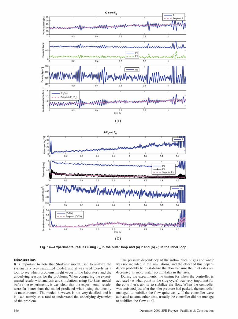
and (f) P2 and FQ. Fig. 11 shows a sketch of a cascade control structure for Alternative (e), and Figs. 12 through 14 show the experimental results for all six alternatives. Figs. 12a through 14a show the results when valve opening z is used as outer-loop measurement. In Figs. 12b through 14b, the measured topside pressure P2 is used.

During the experiments, the operation is gradually moved further into the unstable region by changing the set point in the outer loop (increasing z and decreasing P2). The valve opening for which the flow can no longer be stabilized gives a measure on the performance of each controller. Note that being able to increase the mean valve opening and keep the flow stable at the same time has

(a)

(b)

Fig. 12—Experimental results using P1 in the outer loop and (a) z and (b) P2 in the inner loop.

skoge

Cross-Out

skoge

Replacement Text

inner

skoge

Cross-Out

skoge

Replacement Text

outer


large economic advantages. This is because producing at a higher valve opening implies less friction loss and increased production.

The results using all of the controllers were very good, and they all managed to stabilize the flow far into the unstable region. The upper plot in each of the subfigures shows how the valve opening is increased during the experiments.

Table 2 compares the average values the last 12 minutes before the controllers go unstable. As mentioned, the mean valve opening gives a good indication of the quality of the controller; see also Fig. B-1 in Appendix B, which shows more-detailed plots for all the controllers the last 12 minutes before instability.

On the basis of the results, we conclude that using P2 in the outer loop and either P1 or FQ in the inner loop is the best choice with average maximum valve opening of 23.8 and 23.9%, respec-tively. The third-best choice is using z in the outer loop and FQ in the inner loop (22.8%).

The controllers were not fine tuned, and the results might be influenced somewhat by the quality of the tuning. Still, the results showed that it was possible to stabilize the flow very well using only topside measurements and that these results are comparable to the results found when including subsea measurement P1 as one of the measurements.

(a)

(b)

Fig. 13—Experimental results using � in the outer loop and (a) z and (b) P2 in the inner loop.


Discussion It is important to note that Storkaas’ model used to analyze the system is a very simplified model, and it was used merely as a tool to see which problems might occur in the laboratory and the underlying reasons for the problems. When comparing the experi-mental results with analysis and simulations using Storkaas’ model before the experiments, it was clear that the experimental results were far better than the model predicted when using the density as measurement. The model, however, is not very detailed, and it is used merely as a tool to understand the underlying dynamics of the problem.

The pressure dependency of the inflow rates of gas and water was not included in the simulations, and the effect of this depen-dency probably helps stabilize the flow because the inlet rates are decreased as more water accumulates in the riser.

During the experiments, the timing for when the controller is activated (at what point in the slug cycle) was very important for the controller’s ability to stabilize the flow. When the controller was activated just after the inlet pressure had peaked, the controller managed to stabilize the flow quite easily. If the controller were activated at some other time, usually the controller did not manage to stabilize the flow at all.

(a)

(b)

Fig. 14—Experimental results using FQ in the outer loop and (a) z and (b) P2 in the inner loop.


Also, the tuning of the controllers has a large influence on the results. Even better results might be achieved with other types of controllers or with better tuning. This is also why it is not pos-sible to make a clear recommendation of which combination of measurements is best. The study does, however, show that all the combinations stabilize the flow quite well.

Conclusions This paper has presented results from a medium-scale riser rig where the aim was to control the flow using only topside measurements. The results show that it was possible to “stabilize the flow” (mean-ing that severe slugging was avoided) using different combinations of topside measurements. Table 2 shows the different controller results compared to each other. The best results were achieved with the scaled volumetric-flow rate FQ /Cv as the inner measurements, although this result may be dependent on the tuning of the control-lers. All the controllers managed to stabilize the flow, increasing the maximum valve opening for the onset of slug flow from approxi-mately 12% without control to almost 24% with control.

When comparing the results with similar experiments per-formed on a small-scale riser rig (Sivertsen et al. 2009), the results using different control configurations are quite similar. This sug-gests that the small-scale riser rig might be suitable for testing dif-ferent control strategies before more-costly and -time-consuming tests on larger rigs.

Nomenclature dP, �P = pressure drop FQ = volumetric-fl ow rate FW = mass-fl ow rate LI = separator level measuring instrumentation (Fig. 3) P1 = pressure upstream of the riser P2 = topside pressure z = valve opening � = density

Acknowledgments The authors would like to thank the Statoil Research Centre in Porsgrunn for letting us perform experiments on its test facilities.

Also, we appreciate all the help that was provided by the people working there, in particular Kristin Hestetun for helping with the experiments. Also, the technical staff deserves thanks for helping with the equipment.

ReferencesGodhavn, J.-M., Fard, M.P., and Fuchs, P.H. 2005. New slug control strate-

gies, tuning rules and experimental results. Journal of Process Control 15 (15): 547–557. doi: 10.1016/j.jprocont.2004.10.003.

Sivertsen, H., Storkaas, E., and Skogestad, S. 2009. Small scale experi-ments on stabilizing riser slug flow. Chemical Engineering Research and Design (in press; published online 06 October 2009). doi: 10.1016/j.cherd.2009.08.007.

Skogestad, S. and Postlethwaite, I. 1996. Multivariable Feedback Control: Analysis and Design. West Sussex, UK: John Wiley & Sons.

Storkaas, E., Skogestad, S., and Godhavn, J.-M. 2003. A Low-Dimensional Model of Severe Slugging for Controller Design and Analysis. Multi-phase ’03, San Remo, Italy, 11–13 June.

Appendix A—Modeling and Analysis The process model G and disturbance model Gd were found by linearizing Storkaas’ model at two operation points (z = 0.15 and z = 0.2). The process variables were scaled with respect to the largest allowed control error, and the disturbances were scaled with the largest variations in the inlet-flow rates in the laboratory, as described in Skogestad and Postlethwaite (1996). The disturbances were assumed to be frequency independent. The input was scaled with the maximum allowed positive deviation in valve opening because the process gain is smaller for large valve openings. For measurements y = [P1, P2, �, FW, FQ] the scaling matrix is De = diag[0.1 bar, 0.1 bar, 50 kg/m3, 0.2 kg/s, 1×10−3 m3/s]. The scaling matrix for the disturbances d = [mG and mL] is Dd = diag [2×10−3

kg/s, 0.2 kg/s]. The nominal values are 0.0075 kg/s for the gas and 1.64 kg/s for the water rate. The input is scaled Du = 1−znom, where znom is the nominal valve opening.

Tables A-1 and A-2 summarize the results of the analysis. The locations of the RHP poles and zeros are presented for valve open-ings of 15 and 20%, as well as stationary gain and lower bounds on the closed-loop transfer functions described in Sivertsen et al.

TABLE 2—MEAN VALUES JUST BEFORE INSTABILITY USING DIFFERENT CASCADE CONTROLLERS*

Outer-Loop z Outer-Loop P2

Inner loop P1 FQ/Cv P1 FQ/Cv P1 (barg) 0.71 0.68 0.68 0.72 0.72 0.67 P2 (barg) 0.146 0.123 0.119 0.132 0.142 0.079

(kg/m3) 425 433 403 424 433 417 FQ /Cv 1.18 0.98 1.18 1.28 1.094 0.997 z (%) 20.9 19.5 22.8 23.8 19.3 23.9 FW (kg/h) 7.24 7.55 7.6 7.54 7.60 7.55 FQ (m3/h) 7.53 10.07 9.2 8.17 8.56 11.05 Figure B-1a B-1b B-1c B-1d B-1e B-1f

* Based on data plotted in Figure B-1.

TABLE A-1—CONTROL LIMITATION DATA FOR VALVE OPENING OF 15% (UNSTABLE POLES AT p = 0.0062 ± 0.060i)

Minimum Bounds

Measurement Unstable (RHP) Zeros Stationary gain |G(0)| |S| |SG| |KS| |SGd| |KSGd|

P1 (bar) – 22.9 1.00 0.00 0.16 0.00 0.042 P2 (bar) 1.00, 0.09 20.5 1.21 15.6 0.017 0.054 0.040 (kg/m3) 0.051 33.1 1.22 33.4 0.011 1.02 0.042

FW (kg/s) – 0.00 1.00 0.00 0.006 0.00 0.042 FQ (m3/s) – 8.3 1.00 0.00 0.013 1.02 0.040


(2009). The pole location is independent of the input and output (measurement), but the zeros may move. From the bifurcation plot in Fig. 5, it is seen that both of these valve openings are inside the unstable area. This can also be seen from the RHP location of the poles.

The only two measurements of the ones considered in this paper which introduce RHP zeros into the system are the topside density � and pressure P2. The RHP zeros in both cases are located quite close to the RHP poles, which results in the high peaks especially for sensitivity function SG but also for S. In Fig. A-1, the RHP poles and relevant RHP zeros are plotted together. This plot shows that we can expect problems when trying to stabilize the flow using these measurements as controlled variables.

The model is based on constant inlet-flow rates. The stationary gain for FW predicted by the model is 0, which means that it is not possible to control the steady-state behavior of the system and the system will drift. Usually, the inlet rates are pressure dependent and the zeros for measurements FQ and FW would be expected to be located further away from the origin than indicated by Figs. 2 and 3.

TABLE A-2—CONTROL LIMITATION DATA FOR VALVE OPENING OF 20% (UNSTABLE POLES AT p = 0.019 ± 0.073i)

Minimum Bounds

Measurement Unstable (RHP) Zeros Stationary Gain |G(0)| |S| |SG| |KS| |SGd| |KSGd|

P1 (bar) – 10.1 1.00 0.00 0.082 0.00 0.090 P2 (bar) 1.08, 0.089 8.94 1.66 10.7 0.10 0.055 0.070 (kg/m3) 0.050 2.87 1.60 19.6 0.048 1.27 0.080

FW (kg/s) – 0.00 1.00 0.00 0.021 0.00 0.070 FQ (m3/s) – 4.16 1.00 0.00 0.047 0.00 0.070

Fig. A-1—Plot-zero map for valve opening 20%.

Figs. A-2 and A-3 show the Bode plots for the different plant models and disturbance models, respectively. The models were found from a linearization of the model around a valve opening of 15%. As in Sivertsen et al. (2009), the Bode plots show that, for the mass-flow-rate measurement FW, the low-frequency value of the disturbance model |GdW| is higher than plant model |GW|. For acceptable control, we require |G( jw)| > |Gd( jw)|−1 for frequencies where |Gd| > 1 (Skogestad and Postlethwaite 1996). In this case, |Gd(0)| is 1.01 and GW is close to zero, which means problems can occur for this measurement.

Appendix B—Experimental Results Fig. B-1 shows plots for all the controllers the last 12 minutes before instability.

(a) P1 and z (b) � and z (c) FQ /Cv and z (d) P1 and P2 (e) � and P2 (f) FQ /Cv and P2


Fig. A-2—Bode plots for the plant models using different measurements.

Fig. A-3—Bode plots for the disturbance models using different measurements.


Heidi Sivertsen is a principle production engineer at Statoil in Stjørdal, Norway, working with the Åsgard offshore field. She holds a PhD degree in chemical engineering from the Norwegian University of Science and Technology. Vidar Alstad is a principle researcher at the Statoil Research Centre in Porsgrunn, Norway. His main research interests are multiphase flow and production optimization. He holds a PhD degree in chemical engineering (process control) from the Norwegian University of Science and Technology. Sigurd Skogestad holds a PhD degree from the California Institute of Technology. He has been a full professor at the Norwegian University of

Fig. B-1—Experimental results using six different combinations of measurements, last 12 minutes before instability.

Science and Technology, Trondheim, Norway, since 1987. He is the principal author, together with Ian Postlethwaite, of the book Multivariable Feedback Control, published by Wiley in 1996 (first edition) and 2005 (second edition), and of the book Chemical and Energy Process Engineering (CRC Press 2009). His research interests include the use of feedback as a tool to make the system well-behaved (including self-optimizing control), limitations on performance in linear systems, control structure design and plantwide control, interactions between process design and control, and distillation column design, control, and dynamics.

Documents

Medium-Scale Experiments on Stabilizing Riser-Slug Flow