Embed Size (px)
DESCRIPTION
By M.S. Howe
Citation preview
JOURNAL OFSOUND ANDVIBRATION
www.elsevier.com/locate/jsvi
Journal of Sound and Vibration 273 (2004) 103–123
Mechanism of sound generation by low Mach numberflow over a wall cavity
M.S. Howe*
Boston University, College of Engineering, 110 Cummington Street, Boston, MA 02215, USA
Received 1 November 2002; accepted 26 April 2003
Abstract
An analysis is made of the mechanism of sound production by nominally steady low Mach number flowover a rigid shallow wall cavity. At very low Mach numbers the dominant source of sound is the unsteadydrag, and the aeroacoustic dipole source accompanying this force. A monopole source dependent on thecompression of fluid within the cavity is smaller by a factor of the order of the flow Mach number M: Thedirectivity of the dipole sound peaks in directions upstream and downstream of the cavity, and there is aradiation null in the direction normal to the plane of the wall. However, numerical simulations for M assmall as 0.1 have predicted significant radiation in directions normal to the wall. This anomaly isinvestigated in this paper by means of an acoustic Green’s function tailored to cavity geometry thataccounts for possible aeroacoustic contributions from both the drag-dipole and from the lowest ordercavity resonance. The Green’s function is used to show that these sources are correlated and that theirstrengths are each proportional to the unsteady drag generated by vorticity interacting with the cavitytrailing edge. When MB0:01; the case in most underwater applications, the monopole strength is alwaysnegligible (for a cavity with rigid walls). At low Mach numbers exceeding about 0.05 it is shown that the
cavity monopole radiation is OðM2Þ{1 relative to the dipole at low frequencies. At higher frequencies, nearthe resonance frequency of the cavity, the monopole and dipole have similar orders of magnitude, and thecombination produces a relatively uniform radiation directivity, with substantial energy radiated indirections normal to the wall. Illustrative numerical results are given for a wall cavity subject to ‘shear layermode’ excitation by the Rossiter ‘feedback’ mechanism.r 2003 Elsevier Ltd. All rights reserved.
ARTICLE IN PRESS
*Tel.: 617-484-0656; fax: 617-757-5869.
E-mail address: [email protected] (M.S. Howe).
0022-460X/$ - see front matter r 2003 Elsevier Ltd. All rights reserved.
doi:10.1016/S0022-460X(03)00644-8

1. Introduction
Tonal radiation produced by high Reynolds number mean flow over a rectangular wall cavitywas originally attributed to broadband excitation of cavity acoustic resonances by turbulence inthe shear layer over the cavity mouth [1]. However, oscillations can also be maintained by alaminar mean flow, and laminar flow resonances are often observed to be more intense [2,3].Tones generated by shallow cavities whose depth d o L ¼ streamwise cavity length (Fig. 1)generally bear little or no correspondence to cavity modes and are not usually harmonicallyrelated, but are more closely analogous to the ‘edge’ tones excited when a thin jet impinges on awedge-shaped knife edge, and maintained via a ‘feedback’ mechanism from the wedge to the jetnozzle.A cavity tone of frequency f generated by flow of mean stream velocity U is typically
found to lie within certain well defined bands of the Strouhal numbers fL=U when plottedagainst flowMach number. This is consistent with the ‘feedback’ scheme proposed by Rossiter [1],involving the periodic formation of discrete vortices just downstream of the leading edgeof the cavity, and their subsequent interaction with the trailing edge after convection acrossthe cavity mouth. The impulsive sound generated by this interaction propagates upstreamwithin the cavity and causes the boundary layer to separate just upstream of the leading edge.The travel time of a vortex across the cavityBL=Uc; where the convection velocityUcE0:4U – 0:6U ;and the sound radiates back to the leading edge in time L=c0; where c0 is the speedof sound. The returning sound therefore arrives in time to reinforce periodic shedding provided
ARTICLE IN PRESS
Fig. 1. Schematic configuration of nominally steady, high Reynolds number flow over a rigid, rectangular wall cavity of
depth d and streamwise length L:
M.S. Howe / Journal of Sound and Vibration 273 (2004) 103–123104
f satisfies [1]
L
Uc
þL
c0E
n
f; n ¼ 1; 2;y: ð1Þ
This formula must be adjusted to obtain detailed agreement with experiment [4–6], by replacing nby n � b; where b ðB0:25Þ determines a ‘phase lag’ b=f equal to the time delay between (1) thearrival of a vortex at the trailing edge and the emission of the main acoustic pulse, and (2) thearrival of the sound at the leading edge and the release of new vorticity. If account is also taken ofthe Mach number (i.e. temperature) dependence of the sound speed in the cavity, Rossiter’sequation (1) can be written as
fL
U¼
n � b
fU=Uc þ M=ffiffiffiffiffiffiffiffiffiffiffiffiffiffiffiffiffiffiffiffiffiffiffiffiffiffiffiffiffiffiffiffiffiffiffiffi1þ ðg0 � 1ÞM2=2
pg; n ¼ 1; 2;y; ð2Þ
where M ¼ U=c0 and g0 is the ratio of specific heats of the fluid.Predictions of the feedback formula (2) for shallow, rectangular cavities with d=Lo1 agree well
with observations at M > 0:2 for bE14 and Uc=UE0:6 [6]. The contributions from cavity
resonances are important only for deep cavities, and appear to be unimportant unless d=L > 25;
when resonances can dominate the radiation provided the Strouhal number also satisfies (2). Anextensive discussion of experimental results relating to this and other influences of cavity geometryand mean flow conditions on cavity resonances is given by Ahuja and Mendoza [6] for Machnumbers M > 0:2: Research prior to 1980 is reviewed by Rockwell [4] and by Rockwell andNaudascher [7], and Grace [8] has summarized recent attempts to simulate numerically cavitynoise radiation.Experiments conducted by Gharib and Roshko [9] in water with a nominally steady impinging
mean flow (at UB1 m=s) have shown that Rossiter feedback resonances are related to largefluctuations in the drag experienced by the cavity. They identified two hydrodynamic modes ofcavity flow oscillations: for ‘shorter’ cavities relative to the upstream boundary layer thickness(and, according to later work [10], for lower Mach numbers) the unsteady motion over the cavitymouth has the characteristics of an unstable, thin shear layer (‘shear layer mode’) that generatessound by impingement on the cavity trailing edge, essentially in the manner proposed by Rossiter[1]. Recent numerical studies of two-dimensional cavity flows by Colonius et al. [10] predict strongradiation preferentially in the upstream direction, from a ‘source’ centred on the cavity trailingedge. Three-dimensional numerical simulations performed by Fuglsang and Cain [11] of theacoustic field within a shallow cavity ðL=d ¼ 4:5Þ at M ¼ 0:85 also indicated that shear layerinstability is the main exciting mechanism, and that it produces a source-like periodic additionand removal of mass near the trailing edge. An analytical, but empirical representation of thisedge source had been previously considered by Tam and Block [12]. Flow over longer cavities (or,alternatively, at higher Mach numbers) is characterized by a ‘wake mode’, involving large scalevorticity ejection from the cavity, producing quasi-periodic separation upstream of the leadingedge. The onset of the wake mode is accompanied by a large increase in drag fluctuations. Thisapparently occurs also at much higher Mach numbers. For example, numerical simulations byZhang [13] for L=d ¼ 3 and M ¼ 1:5; 3 reveal that the violent ejection of vorticity is stronglycorrelated with sign reversals of the cavity drag coefficient.
ARTICLE IN PRESS
M.S. Howe / Journal of Sound and Vibration 273 (2004) 103–123 105
The results of the shear layer mode theory of Tam and Block [12] suggested that at very lowMach numbers ðMo0:2Þ cavity acoustic resonances must contribute to the radiation, especiallyfor deeper cavities ðL=do1
2; say); the ‘monopole’ nature of such resonances would account for a
near omni-directional character of the radiation pattern observed at certain frequencies. They didnot pursue this theoretically, although its likely importance had already been anticipated byPlumblee et al. [14] and by East [15]. Similarly, experiments of Yu [16] have confirmed thatshallow wall cavities in air at Mach numbers MB0:1 radiate a substantial amount of radiationdirectly away from the wall. Numerical and experimental studies at low Mach number by Inagakiet al. [17] have confirmed this conclusion for large cavities with small openings to the mean flow,but shown also how coincidence between the cavity resonance and the Rossiter frequencypredicted by (2) resulted in very large amplitude radiation. For shallow cavities trailing edge‘scattering’ of shear layer pressure fluctuations appears to be the dominant source, even whenfeedback is not important. This is in accord with measurements performed by Jacobs et al. [18] forL=d > 7 and Mo0:4; for which the radiation peaked in the upstream and downstream directions,although significant radiation in the wall-normal direction was also observed.According to the theoretical results of Howe [2], the radiation from a shallow cavity at very low
Mach number can be ascribed to a dipole source aligned with the mean flow direction whosestrength is determined by the unsteady drag. The dipole source strength is strongly coupled to thehydrodynamic motions in and near the cavity, but is essentially the same in character for boththe ‘shear layer’ and ‘wake’ modes of the cavity oscillations, provided M is sufficiently small. Theintensity of the dipole radiation peaks in the upstream and downstream directions, and is null indirections normal to the wall.This conclusion is apparently incompatible with several of the experiments discussed above and
with recent numerical simulations and observations at low Mach numbers. In Hardin and Pope’s[19,20] low Mach number scheme, an incompressible representation of the cavity flow is firstsimulated numerically, and the results are then used to evaluate acoustic ‘sources’ in a modifiedsystem of compressible flow equations. At M ¼ 0:1 their predictions yield radiation directivitiesthat peak in the upstream direction, but also exhibit substantial levels in directions normal to thewall, consistent with the presence of a cavity monopole field. Although various details of theapproach in [19,20] have been criticized and subjected to modification, for example byEkaterinaris [21] and by Shen and Sorensen [22], the general characteristics of the predictedradiation are probably correct in an overall sense, if not in detail. Indeed, they accord with laternumerical studies (also based on an initial determination of an incompressible approximation ofthe cavity flow) by Grace et al. [23] and by Curtis Granda [24], that similarly predict largeamplitude radiation normal to the wall.The purpose of the present paper is to resolve these apparent inconsistencies between numerical
and analytical predictions at low Mach numbers. It will be shown that the low Mach numberdipole radiation, peaking in directions upstream and downstream of the cavity, is indeed thedominant source at very low Mach numbers, typically much smaller than M ¼ 0:1; however.Thus, it is this source that determines cavity radiation in underwater applications (whereMB0:01) provided, of course, that the cavity walls are sufficiently ‘rigid’ to preclude monopolesources produced by pulsations in the cavity volume. But, when MB0:1 we shall show that thecavity ‘Helmholtz’ mode, although very weak and formally vanishingly small as fL=U-0;
ARTICLE IN PRESS
M.S. Howe / Journal of Sound and Vibration 273 (2004) 103–123106

supplies an additional, omni-directional contribution that can exceed the drag dipole radiationover a range of frequencies. Furthermore, it will be shown that the monopole and dipole sourcestrengths are both determined at low Mach numbers by the cavity drag fluctuations.The low Mach number analysis will be framed, in terms of the theory of vortex sound [3], and
the relevant equations are recalled in Section 2. The possible source types are identified byintroducing an acoustic Green’s function that is valid in the presence of low Mach number meanstream flow past the cavity (Section 3). At very low Mach numbers the acoustic amplitudes arealways small enough for incompressible flow to be regarded as an excellent first approximation tothe motion in the cavity. This flow determines the effective vortex sound source strengths,irrespective of whether the flow is characterized as ‘shear layer’ or ‘wake’ mode. Predictions of thetheory are therefore illustrated in Section 4 for the simpler case of shear mode flow by means of anidealized model of shear layer excitation.
2. Formulation
Consider nominally steady, low Mach number, high Reynolds number mean flow in thepositive x1 direction of the rectangular coordinates ðx1;x2; x3Þ over the rectangular wall cavity ofFig. 1. The wall and the interior surfaces of the cavity are assumed to be rigid. The fluid has meandensity and sound speed, respectively, equal to r0; c0; and the velocity in the main stream is U :The cavity has depth d and breadth b; and is aligned with its remaining side of length L parallel tothe mean flow. The co-ordinate origin is taken at O in the plane of the wall at the center of thecavity mouth, with the x2-axis normal to the wall and directed into the main stream.Sound is produced by flow instability in the neighborhood of the cavity. According to
Lighthill’s acoustic analogy [3], when the total enthalpy B; say, is taken as the acoustic variable,the radiation can be expressed in terms of sources that represent excitation by vorticity andentropy fluctuations. For a nominally homogeneous flow at low Mach numbers the motion maybe regarded as homentropic to a good approximation [25]. In that case the total enthalpy becomes
B ¼Zdp
rþ 12
v2; ð3Þ
where r is fluid density, p � pðrÞ the pressure, and v denotes velocity, and Lighthill’s acousticanalogy equation becomes
D
Dt
1
c2D
Dt
� ��1
rr ðrrÞ
� �B ¼
1
rdivðrx4vÞ; ð4Þ
where c is the local speed of sound. In the irrotational acoustic far field, Crocco’s form of themomentum equation @v=@t ¼ �rB implies that B ¼ �@j=@t; where jðx; tÞ is the velocitypotential that determines the whole motion in the irrotational regions of the fluid. B is thereforeequal to a constant in a steady mean flow, and at large distances from the sources perturbations inB represent outgoing sound waves.In the particular case of lowMach number flow, whenM ¼ U=c0 is smaller than about 0.2, say,
so that M2{1; the characteristics of the motion within and close to the cavity will be essentiallythe same as if the fluid is incompressible, the acoustic component constituting a very small
ARTICLE IN PRESS
M.S. Howe / Journal of Sound and Vibration 273 (2004) 103–123 107
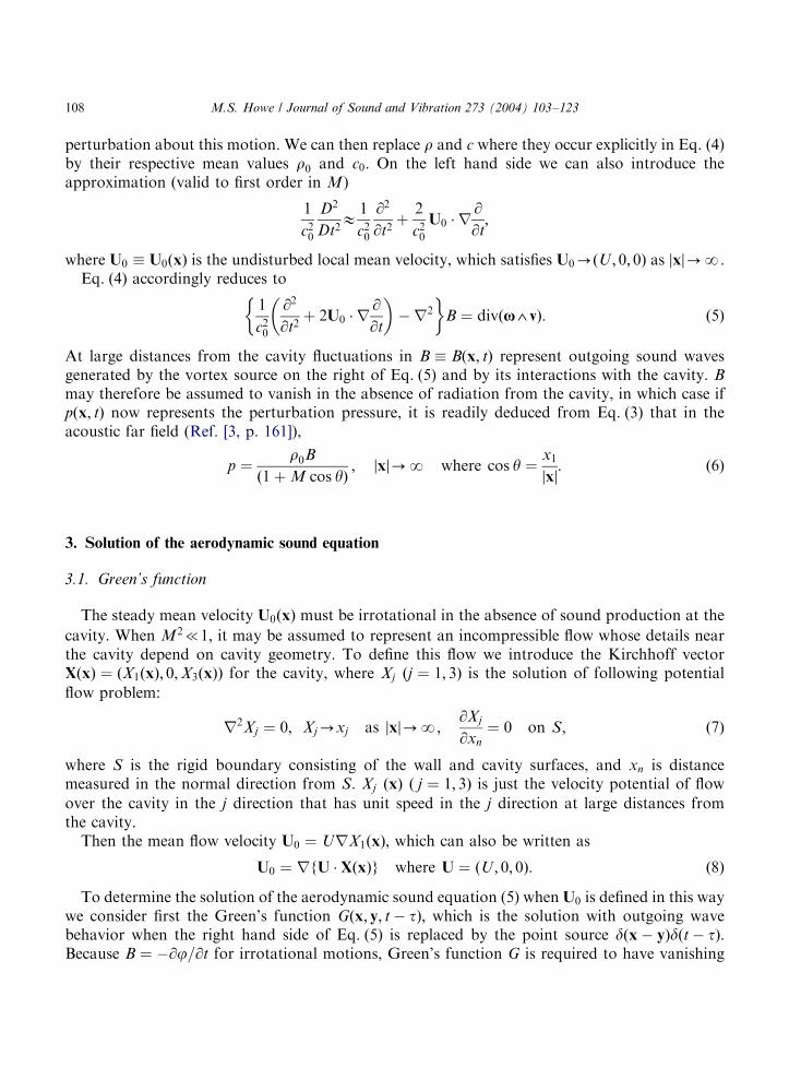
perturbation about this motion. We can then replace r and c where they occur explicitly in Eq. (4)by their respective mean values r0 and c0: On the left hand side we can also introduce theapproximation (valid to first order in M)
1
c20
D2
Dt2E1
c20
@2
@t2þ2
c20U0 r
@
@t;
where U0 � U0ðxÞ is the undisturbed local mean velocity, which satisfies U0-ðU ; 0; 0Þ as jxj-N:Eq. (4) accordingly reduces to
1
c20
@2
@t2þ 2U0 r
@
@t
� ��r2
� �B ¼ divðx4vÞ: ð5Þ
At large distances from the cavity fluctuations in B � Bðx; tÞ represent outgoing sound wavesgenerated by the vortex source on the right of Eq. (5) and by its interactions with the cavity. Bmay therefore be assumed to vanish in the absence of radiation from the cavity, in which case ifpðx; tÞ now represents the perturbation pressure, it is readily deduced from Eq. (3) that in theacoustic far field (Ref. [3, p. 161]),
p ¼r0B
ð1þ M cos yÞ; jxj-N where cos y ¼
x1
jxj: ð6Þ
3. Solution of the aerodynamic sound equation
3.1. Green’s function
The steady mean velocity U0ðxÞ must be irrotational in the absence of sound production at thecavity. When M2{1; it may be assumed to represent an incompressible flow whose details nearthe cavity depend on cavity geometry. To define this flow we introduce the Kirchhoff vectorXðxÞ ¼ ðX1ðxÞ; 0;X3ðxÞÞ for the cavity, where Xj ðj ¼ 1; 3Þ is the solution of following potentialflow problem:
r2Xj ¼ 0; Xj-xj as jxj-N;@Xj
@xn
¼ 0 on S; ð7Þ
where S is the rigid boundary consisting of the wall and cavity surfaces, and xn is distancemeasured in the normal direction from S: Xj ðxÞ ð j ¼ 1; 3Þ is just the velocity potential of flowover the cavity in the j direction that has unit speed in the j direction at large distances fromthe cavity.Then the mean flow velocity U0 ¼ UrX1ðxÞ; which can also be written as
U0 ¼ rfU XðxÞg where U ¼ ðU ; 0; 0Þ: ð8Þ
To determine the solution of the aerodynamic sound equation (5) when U0 is defined in this waywe consider first the Green’s function Gðx; y; t � tÞ; which is the solution with outgoing wavebehavior when the right hand side of Eq. (5) is replaced by the point source dðx� yÞdðt � tÞ:Because B ¼ �@j=@t for irrotational motions, Green’s function G is required to have vanishing
ARTICLE IN PRESS
M.S. Howe / Journal of Sound and Vibration 273 (2004) 103–123108

normal derivative on S: Introduce the transformation [3,26]
Gðx; y; t � tÞ ¼ �1
2p
ZN
�N
#Gðx; y;oÞe�ioðt�tþMðX�YÞ=c0Þ do; ð9Þ
where M ¼ U=c0; and Y ¼ ðY1; 0;Y3Þ is the Kirchhoff vector expressed in terms of y; then whenM2{1; #G satisfies
ðr2 þ k20Þ #G ¼ dðx� yÞ;@ #G
@xn
¼ 0 on S; ð10Þ
where k0 ¼ o=c0 is the acoustic wave number.In the cavity radiation problem the source point y is within or near the cavity, and the
observation point x is in the main stream, at large distances from the cavity. In thesecircumstances an analytical approximation to the solution of Eq. (10) can be derived by a familiar
procedure [3] that involves a straightforward application of the reciprocal theorem #Gðx; y;oÞ ¼#Gðy; x;oÞ [27]: the roles of x and y are interchanged in Eq. (10), which is now to be solved as a
function of y for the reciprocal configuration in which the source is placed at the far field point x:The distant source generates a spherical wave that may be regarded as locally plane when it arrivesat the wall cavity. This greatly simplifies the problem when the characteristic wavelengthB2p=k0of the sound is large compared to the typical cavity dimension, which is the case at sufficientlysmall Mach numbers. We can then anticipate that there are two principal contributions to thecavity response to the impinging wave: a monopole component produced by a periodic volumeflux across the plane of the cavity mouth, corresponding to ‘breathing’ oscillations in the mannerof a Helmholtz resonator [27], and a dipole field, with dipole axis parallel to the plane of the wall,representing an unsteady drag force on the cavity.Therefore, in the usual way [3] for y within and near the cavity and jxj-N; we put
#GE #G0 þ #GM þ #GD; ð11Þ
where #G0 represents the uniform pressure produced by the incident wave in the neighborhood of
the cavity, and #GM and #GD; respectively, represent the monopole and dipole fields near the cavity.In the absence of the cavity the exact Green’s function is
#G ¼ �eik0jx�yj
4pjx� yj�eik0j %x�yj
4pj %x� yj; %x ¼ ðx1;�x2; x3Þ; ð12Þ
which satisfies @ #G=@y2 ¼ 0 on the plane surface y2 ¼ 0 of the wall. When k0jyj{1 and k0jxjc1this becomes
#GE�eik0jxj
2pjxjþik0ðxþ %xÞ y eik0jxj
4pjxj2þy; ð13Þ
where the terms omitted are of orderBðk0jyjÞ2 and smaller. The first term on the right hand side
represents (as a function of y) a uniform pressure fluctuation over the mouth of the cavity and
must therefore correspond to #G0: The second term BOðk0jyjÞ; and satisfies as a function of yLaplace’s equation to this order. It is the velocity potential of a uniform, incompressible flowparallel to the wall (because xþ %x ¼ 2ðx1; 0; x3ÞÞ; and must be augmented by a suitable solution ofLaplace’s equation that accounts for the presence of the cavity (and in particular for the singular
ARTICLE IN PRESS
M.S. Howe / Journal of Sound and Vibration 273 (2004) 103–123 109
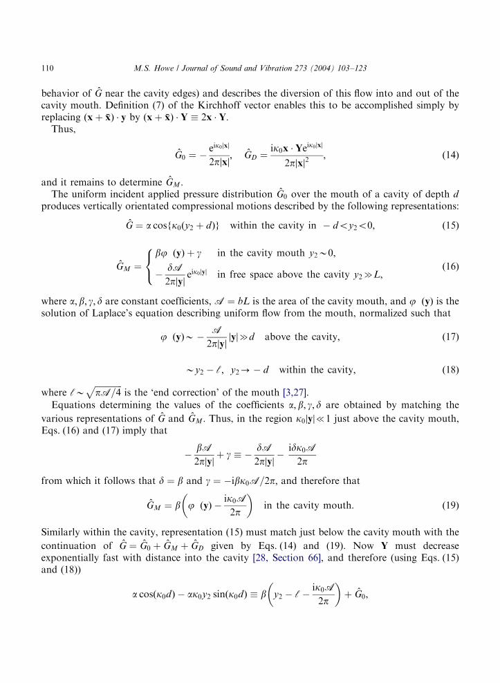
behavior of #G near the cavity edges) and describes the diversion of this flow into and out of thecavity mouth. Definition (7) of the Kirchhoff vector enables this to be accomplished simply byreplacing ðxþ %xÞ y by ðxþ %xÞ Y � 2x Y:Thus,
#G0 ¼ �eik0jxj
2pjxj; #GD ¼
ik0x Yeik0jxj
2pjxj2; ð14Þ
and it remains to determine #GM :The uniform incident applied pressure distribution #G0 over the mouth of a cavity of depth d
produces vertically orientated compressional motions described by the following representations:
#G ¼ a cosfk0ðy2 þ dÞg within the cavity in � doy2o0; ð15Þ
#GM ¼bj�ðyÞ þ g in the cavity mouth y2B0;
�dA2pjyj
eik0jyj in free space above the cavity y2cL;
8<: ð16Þ
where a; b; g; d are constant coefficients,A ¼ bL is the area of the cavity mouth, and j�ðyÞ is thesolution of Laplace’s equation describing uniform flow from the mouth, normalized such that
j�ðyÞB�A
2pjyjjyjcd above the cavity; ð17Þ
By2 � c; y2-� d within the cavity; ð18Þ
where cBffiffiffiffiffiffiffiffiffiffiffiffiffipA=4
pis the ‘end correction’ of the mouth [3,27].
Equations determining the values of the coefficients a; b; g; d are obtained by matching thevarious representations of #G and #GM : Thus, in the region k0jyj{1 just above the cavity mouth,Eqs. (16) and (17) imply that
�bA2pjyj
þ g � �dA2pjyj
�idk0A2p
from which it follows that d ¼ b and g ¼ �ibk0A=2p; and therefore that
#GM ¼ b j�ðyÞ �ik0A2p
� �in the cavity mouth: ð19Þ
Similarly within the cavity, representation (15) must match just below the cavity mouth with the
continuation of #G ¼ #G0 þ #GM þ #GD given by Eqs. (14) and (19). Now Y must decreaseexponentially fast with distance into the cavity [28, Section 66], and therefore (using Eqs. (15)and (18))
a cosðk0dÞ � ak0y2 sinðk0dÞ � b y2 � c�ik0A2p
� �þ #G0;
ARTICLE IN PRESS
M.S. Howe / Journal of Sound and Vibration 273 (2004) 103–123110
from which it follows, in particular, that
#GME j�ðyÞ �ik0A2p
� �eik0jxj
2pjxj1
k0 tanðk0dÞ� c�
ik0A2p
� ��
E j�ðyÞ �ik0A2p
� �k0 sinðk0dÞ
cosfk0ðd þ cþ ik0A=2pÞgeik0jxj
2pjxj: ð20Þ
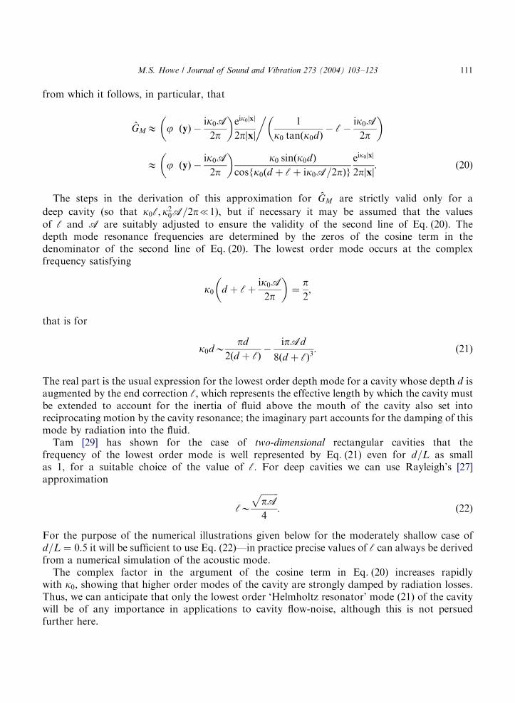
The steps in the derivation of this approximation for #GM are strictly valid only for a
deep cavity (so that k0c; k20A=2p{1), but if necessary it may be assumed that the values
of c and A are suitably adjusted to ensure the validity of the second line of Eq. (20). Thedepth mode resonance frequencies are determined by the zeros of the cosine term in thedenominator of the second line of Eq. (20). The lowest order mode occurs at the complexfrequency satisfying
k0 d þ cþik0A2p
� �¼
p2;
that is for
k0dBpd
2ðd þ cÞ�
ipAd
8ðd þ cÞ3: ð21Þ
The real part is the usual expression for the lowest order depth mode for a cavity whose depth d isaugmented by the end correction c; which represents the effective length by which the cavity mustbe extended to account for the inertia of fluid above the mouth of the cavity also set intoreciprocating motion by the cavity resonance; the imaginary part accounts for the damping of thismode by radiation into the fluid.Tam [29] has shown for the case of two-dimensional rectangular cavities that the
frequency of the lowest order mode is well represented by Eq. (21) even for d=L as smallas 1, for a suitable choice of the value of c: For deep cavities we can use Rayleigh’s [27]approximation
cB
ffiffiffiffiffiffiffiffipA
p4
: ð22Þ
For the purpose of the numerical illustrations given below for the moderately shallow case ofd=L ¼ 0:5 it will be sufficient to use Eq. (22)—in practice precise values of c can always be derivedfrom a numerical simulation of the acoustic mode.The complex factor in the argument of the cosine term in Eq. (20) increases rapidly
with k0; showing that higher order modes of the cavity are strongly damped by radiation losses.Thus, we can anticipate that only the lowest order ‘Helmholtz resonator’ mode (21) of the cavitywill be of any importance in applications to cavity flow-noise, although this is not persuedfurther here.
ARTICLE IN PRESS
M.S. Howe / Journal of Sound and Vibration 273 (2004) 103–123 111

Hence, substituting Eqs. (14) and (20) in Eq. (11), and using the inversion formula (9), it followsthat for y in the neighborhood of the cavity mouth and x in the acoustic far field,
Gðx; y; t � tÞE �1
2p
ZN
�N
ð #G0 þ #GM þ #GDÞðx; y;oÞ e�ioðt�tþMðX�YÞ=c0Þ do
¼1
ð2pÞ2jxj
ZN
�N
1� j�ðyÞ �ik0A2p
� �k0 sinðk0dÞ
cosfk0ðd þ cþ ik0A=2pÞg
�
�ik0x Y
jxj
�e�ioðt�t�jxj=c0þMðX�YÞ=c0Þ do: ð23Þ
To interpret this result, observe first that cavity resonance corresponds to k0dBOð1Þ: At suchfrequencies the second term in the brace brackets of the integrand, involving Y; is not important.The latter becomes significant away from resonances, and then only when the source point y isclose to a cavity edge. The basic assumption is that very high frequencies (in excess of the firstcavity resonance) are irrelevant, and this will be the case when excitation occurs at low Machnumbers.
3.2. The radiated sound
Green’s function (23) now permits the solution of the aerodynamic sound equation (5) , whereB is given by Eq. (6) in the far field, to be expressed in the form [3]
pE�r0
ð1þ M cos yÞ
Zðx4vÞðy; tÞ
@G
@yðx; y; t � tÞ d3y dt; jxj-N; ð24Þ
where the integration is over all values of the retarded time t and the fluid region where thevorticity xa0: There are no contributions from surface integrals over the wall and cavity, onwhich the fluid normal component of velocity and the normal derivative of G both vanish.It follows from this result that only the y-dependent part of the Green’s function (23) need be
used in Eq. (24). Therefore, for small Mach numbers and an acoustically compact source flow, theacoustic pressure given by Eq. (24) can be reduced to the form
pEr0
ð2pÞ2ð1þ M cos yÞjxj
Zðx4vÞðy; tÞ
@
@y
ZN
�N
j�ðyÞ k0 sinðk0dÞcosfk0ðd þ cþ ik0A=2pÞg
�
þik0x
jxj�M
� � Y
�e�ioft�t�ðjxj�MxÞ=c0g do d3y dt; jxj-N: ð25Þ
3.3. Leading edge Kutta condition
In a typical oscillatory cavity flow the region within, above and downstream of the cavity isfilled with vorticity generated by shedding, principally from the leading edge region of the cavity.The length scales of the unsteady hydrodynamic motions induced by this vorticity are comparableto the cavity length L; but the characteristic extent of a coherent region of vorticity is usually verymuch smaller. This means that the main contributions to the volume integral in Eq. (25) are from
those regions where rj� and rYj ðj ¼ 1; 3Þ vary rapidly, sinceRðx4vÞðy; tÞ d3yB0 in regions
ARTICLE IN PRESS
M.S. Howe / Journal of Sound and Vibration 273 (2004) 103–123112

where rj� and rYj can be regarded as constant or as varying very slowly relative to the length
scale of the vorticity.It follows that the cavity edges at which rj� and rYj become infinite are the main sources of
the cavity radiation, and a good estimate of the value of the integral can therefore be obtained byexpanding these derivatives about these edges. In doing this we can explicitly discard anycontributions from the leading edge of the cavity, because the Kutta condition ensures thatacoustic excitation by cavity vorticity interacting with this edge is inhibited by the shedding offresh vorticity [2,3,30–32]. Similarly, the contributions from the side edges of the cavity (parallel tothe mean flow direction) are small, because the vortex source x4v convects predominantly in themean flow direction so that its interaction with the edge is effectively invariant with time (i.e. it is‘silent’). We therefore conclude, in accordance with all previous observations, that it is primarilythe trailing edge of the cavity that is responsible for the radiated sound.Recall that Yj ð j ¼ 1; 3Þ may be interpreted as the velocity potential of a uniform flow over the
cavity in the j-direction. This means that jrY3j{jrY1j at the cavity trailing edge, and thereforethat the contribution from Y3 in Eq. (25) can be discarded. If we now introduce a ‘strip theory’approximation for Y1 in the immediate vicinity of the edge, by equating it to the correspondingvelocity potential for flow over a two-dimensional cavity, which is readily found by conformalmapping, we find (for details see Ref. [3])
Y1ðyÞBC1L1=3Reðz2=3Þ where z ¼ y1 �
L
2þ iy2 and C1 ¼
3
2
ð1� mÞ6EðmÞ
�1=3; ð26Þ
where m is the solution of the equation
Kð1� mÞ � Eð1� mÞEðmÞ
¼d
Lð27Þ
and KðxÞ ¼R p=20 dl=
ffiffiffiffiffiffiffiffiffiffiffiffiffiffiffiffiffiffiffiffiffi1� xsin2l
p; EðxÞ ¼
R p=20
ffiffiffiffiffiffiffiffiffiffiffiffiffiffiffiffiffiffiffiffiffi1� xsin2l
pdl ð0oxo1Þ are complete elliptic
integrals [33].A similar strip-theory calculation reveals that near the trailing edge
j�ðyÞBC2Y1ðyÞ; C2 ¼ 2EðmÞ
4pð1� mÞ
�1=3: ð28Þ
Hence, Eq. (25) becomes
pEr0
ð2pÞ2ð1þ M cos yÞjxj
Zðx4vÞðy; tÞ
@Y1
@yðyÞ d3y
�Z
N
�N
k0C2 sinðk0dÞ
cosfk0ðd þ cþ ik0A=2pÞg
�
þ iðcos y� MÞ�e�ioft�t�ðjxj�MxÞ=c0g do dt; jxj-N; ð29Þ
where Y1 is given by Eq. (26).
ARTICLE IN PRESS
M.S. Howe / Journal of Sound and Vibration 273 (2004) 103–123 113

3.4. Physical interpretation
The first and second terms in the large brackets of Eq. (29) correspond respectively to monopoleand dipole radiation from the cavity. The monopole character of the first term should be obviousfrom the discussion in Section 3.1. To understand the dipole nature of the second term note firstthat Eq. (29) is the acoustic pressure as measured by an observer fixed relative to the cavity, andtherefore moving at speed U in the negative x1 direction relative to the mean stream. Let R be thevector position relative to the cavity of an observer in a reference frame moving with the fluid at
the time of emission of the arriving sound. For such an observer the cavity appears to translate atspeed U in the negative x1 direction. The co-ordinate systems x and R are related by (see Fig. 2)x ¼ RþMR; since an observer fixed relative to the fluid moves a distance U � ðR=c0Þ in the x1direction relative to the cavity during the time of travel R=c0 of the sound from the cavity to theobserver. The following relations are now easily derived for small M:
jxj �M x ¼ jRj; jxj ¼ jRjð1þ M cosYÞ; cos y� M ¼cosY
ð1þ M cosYÞ; ð30Þ
where Y is the angle between the observer direction and the mean flow direction at the time ofemission of the sound.Making these substitutions in Eq. (29) we find, for small M;
pEr0
ð2pÞ2ð1þ M cosYÞ2jRj
Zðx4vÞðy; tÞ
@Y1
@yðyÞ d3y
�Z
N
�N
k0C2 sinðk0dÞ
cosfk0ðd þ cþ ik0A=2pÞgþ
i cosYð1þ M cosYÞ
� �� e�ioft�t�jRj=c0g do dt; jRj-N; ð31Þ
where Y1 is given by Eq. (26). This formula represents the radiation measured by a fixed observerfrom a uniformly translating cavity as being equal to the sum of a monopole amplified by thefamiliar two powers of the Doppler factor 1=ð1þ M cosYÞ together with a surface interactiondipole magnified by three Doppler factors (cf. [34]).The strengths of the monopole and dipole sources are both determined by the value of the
integral
FðtÞ ¼ r0
Zðx4vÞðy; tÞ
@Y1
@yðyÞ d3y; ð32Þ
ARTICLE IN PRESS
Fig. 2. Illustrating the relation between the co-ordinate systems x and R:
M.S. Howe / Journal of Sound and Vibration 273 (2004) 103–123114
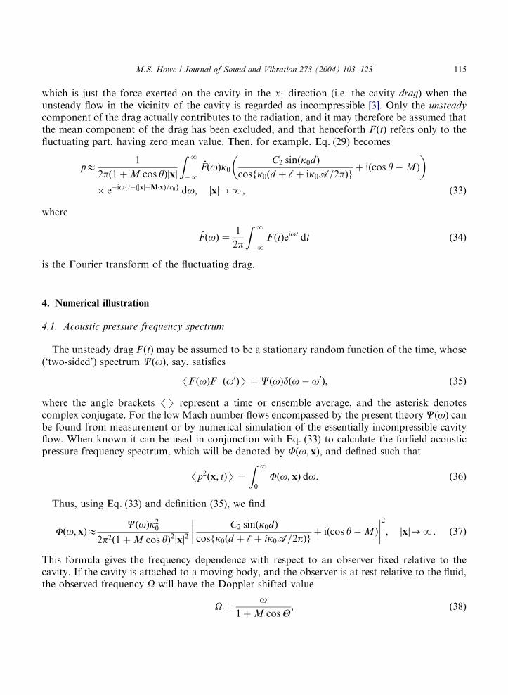
which is just the force exerted on the cavity in the x1 direction (i.e. the cavity drag) when theunsteady flow in the vicinity of the cavity is regarded as incompressible [3]. Only the unsteadycomponent of the drag actually contributes to the radiation, and it may therefore be assumed thatthe mean component of the drag has been excluded, and that henceforth F ðtÞ refers only to thefluctuating part, having zero mean value. Then, for example, Eq. (29) becomes
pE1
2pð1þ M cos yÞjxj
ZN
�N
#FðoÞk0C2 sinðk0dÞ
cosfk0ðd þ cþ ik0A=2pÞgþ iðcos y� MÞ
� �� e�ioft�ðjxj�MxÞ=c0g do; jxj-N; ð33Þ
where
#FðoÞ ¼1
2p
ZN
�N
F ðtÞeiot dt ð34Þ
is the Fourier transform of the fluctuating drag.
4. Numerical illustration
4.1. Acoustic pressure frequency spectrum
The unsteady drag F ðtÞ may be assumed to be a stationary random function of the time, whose(‘two-sided’) spectrum CðoÞ; say, satisfies
/F ðoÞF�ðo0ÞS ¼ CðoÞdðo� o0Þ; ð35Þ
where the angle brackets /S represent a time or ensemble average, and the asterisk denotescomplex conjugate. For the low Mach number flows encompassed by the present theoryCðoÞ canbe found from measurement or by numerical simulation of the essentially incompressible cavityflow. When known it can be used in conjunction with Eq. (33) to calculate the farfield acousticpressure frequency spectrum, which will be denoted by Fðo;xÞ; and defined such that
/p2ðx; tÞS ¼Z
N
0
Fðo;xÞ do: ð36Þ
Thus, using Eq. (33) and definition (35), we find
Fðo; xÞECðoÞk20
2p2ð1þ M cos yÞ2jxj2C2 sinðk0dÞ
cosfk0ðd þ cþ ik0A=2pÞgþ iðcos y� MÞ
��������2
; jxj-N: ð37Þ
This formula gives the frequency dependence with respect to an observer fixed relative to thecavity. If the cavity is attached to a moving body, and the observer is at rest relative to the fluid,the observed frequency O will have the Doppler shifted value
O ¼o
1þ M cosY; ð38Þ
ARTICLE IN PRESS
M.S. Howe / Journal of Sound and Vibration 273 (2004) 103–123 115
so that if /p2ðR; tÞS ¼RN
0 FðO;RÞ dO; then
FðO;RÞECðoÞk20
2p2ð1þ M cosYÞ3jRj2C2 sinðk0dÞ
cosfk0ðd þ cþ ik0A=2pÞgþ
i cosYð1þ M cosYÞ
��������2
; jRj-N; ð39Þ
in which o and k0 ¼ o=c0 are defined in terms of O as in Eq. (38).
4.2. Analytical model for shear layer mode radiation
To illustrate predictions of Eq. (37) a simple yet mathematically tractable model will now beconsidered for a shallow cavity subject to shear layer mode excitation. The principal aerodynamicsources divðx4vÞ on the right of Eq. (5) are then confined to the region above the cavity mouth.In a first approximation the flow is parallel to the x1 direction, so that the main contribution tothe drag integral (32) (wherein Y1 is given approximately by Eq. (26)) is determined by thespanwise component o3 of the vorticity.We therefore write
ðx4vÞðy; tÞEjZ
N
�N
Fðk; k>;o; y2Þeiðky1þk>y3�otÞ dk dk> do; y2 > 0; jy3job
2; ð40Þ
where j is a unit vector in the x2 direction, normal to the plane of the wall, and Fðk; k>;o; y2Þdetermines the distribution across the shear layer of harmonic constituents of the unsteady shearflow of frequency o and with streamwise and spanwise wavelengths, respectively, equal to 2p=k
and 2p=k>: Inserting this formula into the integral of Eq. (32), and using the local approximation
(26) for Y1; the y1-integral is readily evaluated to yield the Fourier transform #FðoÞ of the unsteadydrag in the form
#FðoÞ ¼C1Gð23ÞL
1=3ffiffiffi3
p r0
ZFðk; k>;o; y2Þ
ðk � i0Þ2=3eiðk>y3�p=3Þ�jkjy2 dk dk> dy2 dy3; ð41Þ
where the notation ‘�i0’ implies that the branch cut for ðk � i0Þ2=3 is to be taken from k ¼ 0 toþiN in the upper half-plane.This result can be cast in a more useful form in terms of the hydrodynamic pressure fluctuations
ps; say, that the same flow would exert on the rigid wall in the absence of the cavity. This is usuallycalled the ‘blocked surface pressure’, and in a first approximation may be identified with the(measurable) wall surface pressure fluctuations just downstream of the cavity. At low Machnumbers we can regard this pressure as that generated by the shear layer vorticity when the flow isincompressible, and it is therefore determined by the incompressible form of Eq. (4),
r2B ¼ �divðx4vÞ; x2 > 0 where ps ¼ r0B on x2 ¼ 0: ð42Þ
When x4v is given by Eq. (40) a routine calculation [3] yields
ps ¼Z
N
�N
#psðk; k>;oÞeiðky1þk>y3�otÞ dk dk> do; ð43Þ
where
#psðk; k>;oÞ ¼r02
ZN
0
Fðk; k>;o; y2Þe�fk2þk2>g1=2y2 dy2: ð44Þ
ARTICLE IN PRESS
M.S. Howe / Journal of Sound and Vibration 273 (2004) 103–123116
Now kBo=Uc at those values of the wave number k where the blocked pressure Fourieramplitude #psðk; k>;oÞ is significant. Because the motion over the cavity can be regarded as locallytwo-dimensional, the corresponding typical values of the spanwise wave number k>{k: Thus,
fk2 þ k2>g1=2 can be replaced by jkj in the exponential of Eq. (44), and it is then deduced fromEq. (41) that
#FðoÞE2C1Gð23ÞL
1=3ffiffiffi3
p Z#psðk; k>;oÞ
ðk � i0Þ2=3eiðk>y3�p=3Þ dk dk> dy3: ð45Þ
For stationary random flow we also have [3]
/ #psðk; k>;oÞ #p�s ðk0; k0
>;o0ÞS ¼ Pðk; k>;oÞdðk � k0Þdðk> � k0>Þdðo� o0Þ; ð46Þ
where Pðk; k>;oÞ is the blocked pressure wave number frequency spectrum. Hence, by formingthe product / #FðoÞ #F�ðo0ÞS from Eq. (45), using Eq. (46), and making the further assumption thatthe spanwise correlation length of the unsteady motions is small compared to the cavity width b;we deduce from definition (35), that
CðoÞE8pC2
1G2ð23ÞbL2=3
3
ZN
�N
Pðk; 0;oÞ dk
jkj4=3; ð47Þ
and therefore that the far field acoustic pressure spectrum (37) can be written as
Fðo;xÞE4C2
1G2ð23ÞbL2=3k20
3pð1þ M cos yÞ2jxj2C2 sinðk0dÞ
cosfk0ðd þ cþ ik0A=2pÞgþ iðcos y� MÞ
��������2
�Z
N
�N
Pðk; 0;oÞ dk
jkj4=3; jxj-N: ð48Þ
The functional form of Pðk; 0;oÞ can, in principle, be estimated from measurements of the wallpressure fluctuations just downstream of the trailing edge of the cavity, provided it is permissibleto assume that the statistical properties of the shear layer motions near the trailing edge of thecavity are well approximated by those immediately downstream of the cavity.As an alternative approximate procedure, however, it will be assumed that Pðk; 0;oÞ is sharply
peaked at k ¼ o=Uc; which is the expected behavior when the dominant vortical disturbancesconvect at speed Uc: The integral in Eq. (48) may then be evaluated by replacing jkj by o=Uc in the
denominator, and setting c3FppðoÞ=p ¼RN
�NPðk; 0;oÞ dk; where FppðoÞ is the frequency spectrum
of the wall blocked pressure fluctuations, and c3{b is the spanwise correlation length. Therefore,
Fðo; xÞE4C2
1G2ð23ÞbL2=3
3p2ð1þ M cos yÞ2jxj2c3k20FppðoÞ
ðo=UcÞ4=3
C2 sinðk0dÞcosfk0ðd þ cþ ik0A=2pÞg
þ iðcos y� MÞ����
����2
;
jxj-N: ð49Þ
Consider a case (typical of low Mach number flow over a shallow cavity) where the pressurefluctuations near the cavity peak at the frequency of the second Rossiter mode, near fL=U ¼ 1:Let the functional form of FppðoÞ be approximated by the following empirical formula [3] for
ARTICLE IN PRESS
M.S. Howe / Journal of Sound and Vibration 273 (2004) 103–123 117
turbulent boundary layer flow:
FppðoÞðU=d�Þ
ðr0v2�Þ2
Eðod�=UÞ2
fðod�=UÞ2 þ a2pg3=2
; ap ¼ 0:12; c3E1:4Uc
o: ð50Þ
In this formula d� is the effective displacement thickness of the boundary layer flow, but will beassigned the value
d� ¼Lap
pffiffiffi2
p ; ð51Þ
to ensure that the spectral peak occurs at f L=U ¼ 1: The velocity v� is the nominal frictionvelocity of the wall flow, but its precise value is not required for the present illustrations.In non-dimensional form we may now write
Fðo;xÞðU=d�Þ
ðr0v2�Þ2ðL=jxjÞ2
,5:6C2
1G2ð23Þ
3p2d�L
� �1=3b
L
� �Uc
U
� �7=3
EM2ðod�=UÞ5=3
ð1þ M cos yÞ2fðod�=UÞ2 þ a2pg3=2
C2 sinðk0dÞcosfk0ðd þ cþ ik0A=2pÞg
þ iðcos y� MÞ����
����2
: ð52Þ
Thus, the mean square acoustic pressure scales as ðr0U2Þ2M2; and the overall acoustic intensity
varies as r0U3M3: This is the expected behavior for an aeroacoustic dipole source; in our case the
source is modified by the cavity monopole, but we shall see below that the maximal strength of themonopole is of the same dipole order.Typical plots of the far field acoustic spectrum
10� log10Fðo; xÞðU=d�Þ
ðr0v2�Þ2ðL=jxjÞ2
,5:6C2
1G2ð23Þ
3p2d�L
� �1=3b
L
� �Uc
U
� �7=3( )
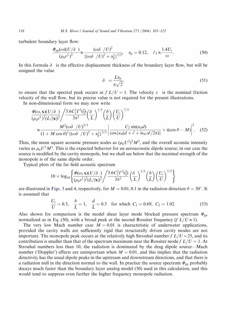
are illustrated in Figs. 3 and 4, respectively, forM ¼ 0:01; 0:1 in the radiation direction y ¼ 30�: Itis assumed that
Uc
U¼ 0:5;
b
L¼ 1;
d
L¼ 0:5 for which C1 ¼ 0:69; C2 ¼ 1:02: ð53Þ
Also shown for comparison is the model shear layer mode blocked pressure spectrum Fpp
normalized as in Eq. (50), with a broad peak at the second Rossiter frequency ðf L=UE1Þ:The very low Mach number case M ¼ 0:01 is characteristic of underwater applications,
provided the cavity walls are sufficiently rigid that structurally driven cavity modes are notimportant. The monopole peak occurs at the relatively high Strouhal number f L=UB25; and itscontribution is smaller than that of the spectrum maximum near the Rossiter mode f L=U ¼ 1: AtStrouhal numbers less than 10, the radiation is dominated by the drag dipole source—Machnumber (‘Doppler’) effects are unimportant when M ¼ 0:01; and this implies that the radiationdirectivity has the usual dipole peaks in the upstream and downstream directions, and that there isa radiation null in the direction normal to the wall. In practice the source spectrum Fpp probably
decays much faster than the boundary layer analog model (50) used in this calculation, and thiswould tend to suppress even further the higher frequency monopole radiation.
ARTICLE IN PRESS
M.S. Howe / Journal of Sound and Vibration 273 (2004) 103–123118
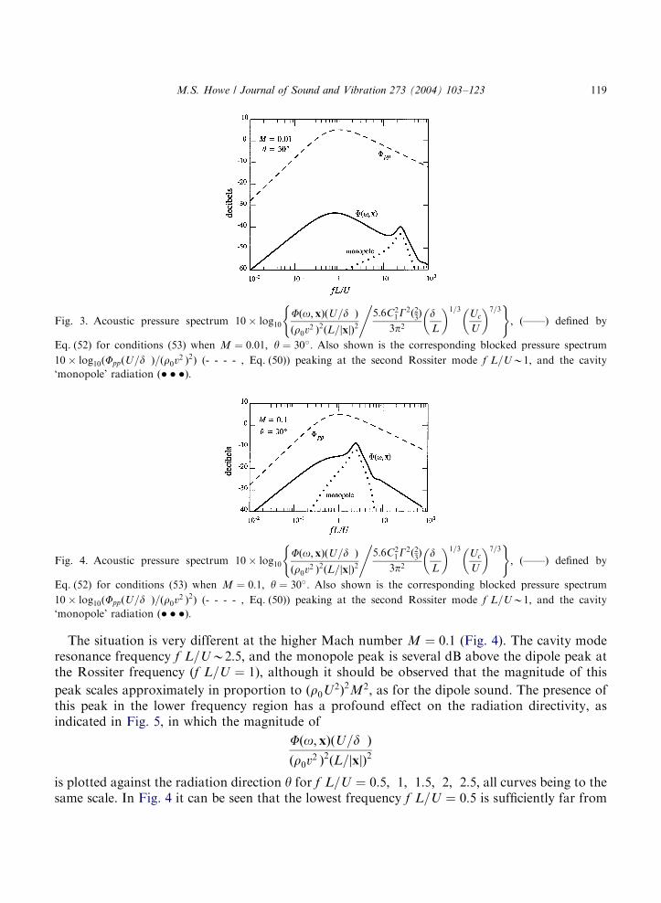
The situation is very different at the higher Mach number M ¼ 0:1 (Fig. 4). The cavity moderesonance frequency f L=UB2:5; and the monopole peak is several dB above the dipole peak atthe Rossiter frequency ðf L=U ¼ 1Þ; although it should be observed that the magnitude of thispeak scales approximately in proportion to ðr0U
2Þ2M2; as for the dipole sound. The presence ofthis peak in the lower frequency region has a profound effect on the radiation directivity, asindicated in Fig. 5, in which the magnitude of
Fðo;xÞðU=d�Þ
ðr0v2�Þ2ðL=jxjÞ2
is plotted against the radiation direction y for f L=U ¼ 0:5; 1; 1:5; 2; 2:5; all curves being to thesame scale. In Fig. 4 it can be seen that the lowest frequency f L=U ¼ 0:5 is sufficiently far from
ARTICLE IN PRESS
Fig. 3. Acoustic pressure spectrum 10� log10Fðo; xÞðU=d�Þ
ðr0v2�Þ2ðL=jxjÞ2
,5:6C2
1G2ð23Þ
3p2d�L
� �1=3Uc
U
� �7=3( ); (——) defined by
Eq. (52) for conditions (53) when M ¼ 0:01; y ¼ 30�: Also shown is the corresponding blocked pressure spectrum
10� log10ðFppðU=d�Þ=ðr0v2�Þ2Þ (- - - - , Eq. (50)) peaking at the second Rossiter mode f L=UB1; and the cavity
‘monopole’ radiation ð� � �Þ:
Fig. 4. Acoustic pressure spectrum 10� log10Fðo; xÞðU=d�Þ
ðr0v2�Þ2ðL=jxjÞ2
,5:6C2
1G2ð23Þ
3p2d�L
� �1=3Uc
U
� �7=3( ); (——) defined by
Eq. (52) for conditions (53) when M ¼ 0:1; y ¼ 30�: Also shown is the corresponding blocked pressure spectrum
10� log10ðFppðU=d�Þ=ðr0v2�Þ2Þ (- - - - , Eq. (50)) peaking at the second Rossiter mode f L=UB1; and the cavity
‘monopole’ radiation ð� � �Þ:
M.S. Howe / Journal of Sound and Vibration 273 (2004) 103–123 119

the monopole peak to be effectively uninfluenced by the monopole. The directivity is thereforethat of a dipole, peaking in the upstream and downstream directions, but subject to Doppleramplification by the mean flow, which causes the level to be larger in upstream directions. Thedotted curves in Figs. 3 and 4 represent the field of the monopole cavity mode alone, when theterm iðcos y� MÞ on the right of Eq. (52) is deleted. This shows that the influence of themonopole is confined to the immediate vicinity of the resonance frequency. At higher frequenciesthe detailed directivity is determined by phase interference between the monopole and dipole, aswell as the differences in the Doppler effects on both sources. Thus, at the spectral peak atf L=U ¼ 2:5 this interference produces strong radiation preferentially in the downstreamdirection.An overall picture of the farfield radiation is obtained by integrating the spectrum (52) with
respect to o: The integral is convergent at o ¼ þN; but contributions at very high frequencies areprobably not representative. Therefore we depict in Fig. 6 forM ¼ 0:05; 0:1 the radiated pressuredirectivity when the integration is confined to the Strouhal number range 0:1of L=Uo10: Inboth cases this includes the frequency range in which the monopole is important. At the lowerMach number the directivity resembles that of a dipole, but peaking in the downstream directionowing to modifications produced by the monopole resonant response. The situation at M ¼ 0:1 issimilar except that there is significant radiation in directions normal to the wall.
ARTICLE IN PRESS
Fig. 6. Directivity 10� log10ð/p2ðx; tÞS=p20Þ of overall sound radiated in the frequency range 0:1of L=Uo10 forM ¼ 0:05; 0:1 for the cavity defined by Eq. (53).
Fig. 5. DirectivityFðo; xÞðU=d�Þ
ðr0v2�Þ2ðL=jxjÞ2
for a cavity of dimensions (53) for M ¼ 0:1 and f L=U ¼ 0:5; 1; 1:5; 2; 2:5 when
the shear layer blocked pressure spectrum Fpp peaks at the second Rossiter mode f L=UB1:
M.S. Howe / Journal of Sound and Vibration 273 (2004) 103–123120

5. Conclusion
At very low Mach numbers the aerodynamic sound generated by nominally steady flow over ashallow wall cavity is dominated by dipole radiation produced by the unsteady drag force, theradiation peaking in directions upstream and downstream of the cavity. The drag force fluctuationsare produced by the interaction of vorticity, in an unstable mean shear layer or periodically ejectedfrom the cavity, with the trailing edge of the cavity. It is the principal source in underwaterapplications where M rarely exceeds about 0.01, provided it is permissible to ignore structuralresonances associated with hydrodynamic forcing of flexing cavity walls. In such cases the lowest,rigid body cavity resonance frequency (the ‘Helmholtz’ resonance frequency) tends to be large, andbeyond the range where it can be effectively excited by the flow. At higher Mach numbers,however, the resonance frequency lies closer to the relevant ‘Rossiter’ modes of the unstablehydrodynamic flow over the cavity, and can then make a significant contribution to the radiation.The cavity resonance produces a monopole contribution to the sound and is governed by
compressible effects in the cavity region. At low Mach numbers these are usually very weak, suchthat whereas the intensity of the drag dipole exhibits the usual aeroacoustic dipole strength
Br0U3M3; the strength of the compressible-dominated, cavity source would vary asBr0U
3M5:However, when significant excitation of the cavity resonance occurs, say at Mach numbersexceeding about 0.05, the unsteady drag fluctuations also excite the cavity mode with a radiationintensity of the same order as the dipole sound. At these higher Mach numbers the radiationdirectivity at a frequency close to the cavity resonance is governed by the correlated interferencebetween the dipole and monopole fields; at frequencies far removed from the resonance thedirectivity reverts to that of an isolated dipole. The overall sound power now tends to beuniformly distributed in direction; in particular there is significant radiation in the directionnormal to the wall, which is otherwise a radiation null for the dipole alone.The detailed results given in this paper are for a moderately shallow cavity dominated by shear
layer mode instabilities, of the kind usually associated with the Rossiter modes. However, theGreen’s function developed in Section 3 can also be used to determine the cavity radiation for veryshallow cavities, where an unsteady hydrodynamic ‘wake flow’ wets the cavity base, and themotion is characterized by the quasi-periodic ejection of cavity vorticity into the main flow. Thisejection produces a violent fluctuation in the drag, which determines both the dipole andmonopole sources of sound.
Acknowledgements
The work reported in this paper is supported by the Office of Naval Research under GrantN00014-02-1-0549 administered by Dr. L. Patrick Purtell. The author gratefully acknowledges thebenefit of discussions with Dr. William K. Blake.
References
[1] J.E. Rossiter, The effect of cavities on the buffeting of aircraft, Royal Aircraft, Establishment Tech. Memo. 754,
1962.
ARTICLE IN PRESS
M.S. Howe / Journal of Sound and Vibration 273 (2004) 103–123 121

[2] M.S. Howe, Edge, cavity and aperture tones at very low Mach numbers, Journal of Fluid Mechanics 330 (1997)
61–84.
[3] M.S. Howe, Acoustics of Fluid-structure Interactions, Cambridge University Press, Cambridge, 1998.
[4] D. Rockwell, Oscillations of impinging shear layers, American Institute of Aeronautics and Astronautics Journal 21
(1983) 645–664.
[5] N.M. Komerath, K.K. Ahuja, F.W. Chambers, Prediction and measurement of flows over cavities—a survey,
American Institute of Aeronautics and Astronautics Paper 87-022, 1987.
[6] K.K. Ahuja, J. Mendoza, Effects of cavity dimensions, boundary layer, and temperature on cavity noise with
emphasis on benchmark data to validate computational aeroacoustic codes, NASA Contractor Report 4653, Final
Report Contract NAS1-19061, Task 13, 1995.
[7] D. Rockwell, E. Naudascher, Review—self-sustaining oscillation of flow past cavities, Transactions of the
American Society of Mechanical Engineers, Journal of Fluids Engineering 100 (1978) 152–165.
[8] S.M. Grace, An overview of computational aeroacoustic techniques applied to cavity noise prediction, American
Institute of Aeronautics and Astronautics Paper 2001-0510, 2001.
[9] M. Gharib, A. Roshko, The effect of flow oscillations on cavity drag, Journal of Fluid Mechanics 177 (1987)
501–530.
[10] T. Colonius, A. Basu, C. Rowley, Numerical investigation of flow past a cavity, American Institute of Aeronautics
and Astronautics Paper 99-1912, 1999.
[11] D.F. Fuglsang, A.B. Cain, Evaluation of shear layer cavity resonances by numerical simulation, American
Institute of Aeronautics and Astronautics Paper 92-0555, 1992.
[12] C.K.W. Tam, P.J.W. Block, On the tones and pressure oscillations induced by flow over rectangular cavities,
Journal of Fluid Mechanics 89 (1978) 373–399.
[13] X. Zhang, Compressive cavity flow oscillations due to shear layer instabilities and pressure feedback, American
Institute of Aeronautics and Astronautics Journal 33 (1995) 1404–1411.
[14] H.E. Plumblee, J.S. Gibson, L.W. Lassiter, A theoretical and experimental investigation of the acoustic response of
cavities in an aerodynamic flow, US Air Force Report WADD-TR-61-75, 1962.
[15] L.F. East, Aerodynamically induced resonance in rectangular cavities, Journal of Sound and Vibration 3 (1966)
277–287.
[16] Y.H. Yu, Measurements of sound radiation from cavities at subsonic speeds, American Institute of Aeronautics
and Astronautics Paper 76-529, 1976.
[17] M. Inagaki, O. Murata, T. Kondoh, Numerical prediction of fluid-resonant oscillation at low Mach number,
American Institute of Aeronautics and Astronautics Journal 40 (2002) 1821–1829.
[18] M. Jacob, V. Gradoz, A. Louisot, S. Juve, S. Guerrand, Comparison of sound radiated by shallow cavities and
backward facing steps. American Institute of Aeronautics and Astronautics Paper 99-1892, 1999.
[19] J.C. Hardin, D.S. Pope, An acoustic/viscous splitting technique for computational aeroacoustics, Theoretical and
Computational Aeroacoustics 6 (1994) 323–340.
[20] J.C. Hardin, D.S. Pope, Sound generation by flow over a two-dimensional cavity, American Institute of
Aeronautics and Astronautics Journal 33 (1995) 407–412.
[21] J.A. Ekaterinaris, New formulation of Hardin–Pope equations for aeroacoustics, American Institute of Aeronautics
and Astronautics Journal 37 (1999) 1033–1039.
[22] W.Z. Shen, J.N. Sorensen, Comment on the aeroacoustic formulation of Hardin and Pope, American Institute of
Aeronautics and Astronautics Journal 37 (1999) 141–143.
[23] S.M. Grace, C.K. Curtis, Acoustic computations using incompressible inviscid CFD results as input, Proceedings
of the ASME Noise Control and Acoustics Division NCA, Vol. 26, ASME IMECE, Nashville, TN, November 1999.
[24] C. Curtis Granda, A Computational Acoustic Prediction Method Applied to Two-dimensional Cavity Flow,
Master’s Thesis, Boston University, December, 2001.
[25] G.K. Batchelor, An Introduction to Fluid Dynamics, Cambridge University Press, Cambridge, 1967.
[26] K. Taylor, A transformation of the acoustic equation with implications for wind tunnel and low speed flight tests,
Proceedings of the Royal Society of London A363 (1978) 271–281.
[27] Lord Rayleigh, Theory of Sound, Vol. 2, Dover, New York, 1945.
[28] Horace Lamb, Hydrodynamics, 6th Edition, Cambridge University Press, Cambridge, 1932.
ARTICLE IN PRESS
M.S. Howe / Journal of Sound and Vibration 273 (2004) 103–123122

[29] C.K.W. Tam, The acoustic modes of a two-dimensional rectangular cavity, Journal of Sound and Vibration 49
(1976) 353–364.
[30] M.S. Howe, The influence of vortex shedding on the generation of sound by convected turbulence, Journal of Fluid
Mechanics 76 (1976) 711–740.
[31] D.G. Crighton, The Kutta condition in unsteady flow, Annual Reviews of Fluid Mechanics 17 (1985) 411–445.
[32] T. Takaishi, A. Sagawa, K. Nagakura, T. Maeda, Numerical analysis of dipole sound source around high speed
trains, Journal of the Acoustical Society of America 111 (2002) 2601–2608.
[33] M. Abramowitz, I.A. Stegun (Eds.), Handbook of Mathematical Functions, 9th Edition, National Bureau of
Standards Applied Mathematics Series No. 55, US Department of Commerce, 1970.
[34] D.G. Crighton, Scattering and diffraction of sound by moving bodies, Journal of Fluid Mechanics 72 (1975)
209–227.
ARTICLE IN PRESS
M.S. Howe / Journal of Sound and Vibration 273 (2004) 103–123 123
![Mach number P w,test [bar] P model [bar] 1.8 -0.45 -0.20 0 ...ae342/18/lab2/lab2data.pdf · Mach 2.0 Snapshot . Mach 1.8 Snapshot . Mach 2.3 Snapshot Mach 2.2 Snapshot . P w,test](https://img.dokumen.tips/doc/110x75/5fb4e5220b26be1bae0aea08/mach-number-p-wtest-bar-p-model-bar-18-045-020-0-ae34218lab2-.jpg)


![DETAILED OBSERVATIONS ON A STARTING MECHANISM … · super-cavitation with clear cavity surface and cavity pressure near vapor one [14]. In the transition stage, namely from sub-](https://img.dokumen.tips/doc/110x75/5b4f640d7f8b9a346e8c3145/detailed-observations-on-a-starting-mechanism-super-cavitation-with-clear-cavity.jpg)