MECH300H Introduction to Finite Element Methods

Lecture 7

Finite Element Analysis of 2-D Problems

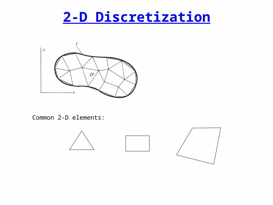
2-D Discretization

Common 2-D elements:

2-D Model Problem with Scalar Function- Heat Conduction

• Governing Equation

0),(),(),(

yxQy

yxT

yx

yxT

x in

• Boundary Conditions

Dirichlet BC:

Natural BC:

Mixed BC:

Weak Formulation of 2-D Model Problem

• Weighted - Integral of 2-D Problem -----

• Weak Form from Integration-by-Parts -----

0 ( , )w T w T

wQ x y dxdyx x y y

T Tw dxdy w dxdy

x x y y

( , ) ( , )( , ) 0

T x y T x yw Q x y dA

x x y y

Weak Formulation of 2-D Model Problem• Green-Gauss Theorem -----

where nx and ny are the components of a unit vector, which is normal to the boundary .

x

T Tw dxdy w n ds

x x x

sinjcosijninn yx

y

T Tw dxdy w n ds

y y y

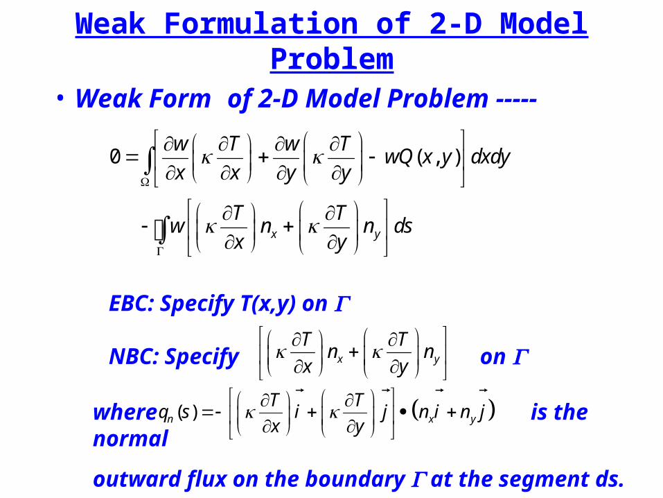
Weak Formulation of 2-D Model Problem

• Weak Form of 2-D Model Problem -----

0 ( , )w T w T

wQ x y dxdyx x y y

x y

T Tw n n ds

x y

EBC: Specify T(x,y) on

NBC: Specify on x y

T Tn n

x y

where is the normal

outward flux on the boundary at the segment ds.

( )n x y

T Tq s i j n i n j

x y

FEM Implementation of 2-D Heat Conduction – Shape Functions

Step 1: Discretization – linear triangular element

T1

T2

T3

332211 TTTT

Derivation of linear triangular shape functions:

Let ycxcc 2101

Interpolation properties

1 at node

0 at other nodesi

i

ith

0 1 1 2 1

0 1 2 2 2

0 1 3 2 3

1

0

0

c c x c y

c c x c y

c c x c y

1

0 1 1

1 2 2

2 3 3

1 1

1 0

1 0

c x y

c x y

c x y

1

1 1 2 3 3 2

1 2 2 2 3

3 3 3 2

1 11

1 1 02

1 0 e

x y x y x yx y

x y x y y yA

x y x x

Same 3 1 1 3

2 3 1

1 3

1

2 e

x y x yx y

y yA

x x

1 2 2 1

3 1 2

2 1

1

2 e

x y x yx y

y yA

x x

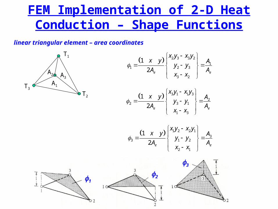
FEM Implementation of 2-D Heat Conduction – Shape Functions

linear triangular element – area coordinates

T1

T2

T3

2 3 3 2

11 2 3

3 2

1

2 e e

x y x yx y A

y yA A

x x

3 1 1 3

22 3 1

1 3

1

2 e e

x y x yx y A

y yA A

x x

1 2 2 1

33 1 2

2 1

1

2 e e

x y x yx y A

y yA A

x x

A3

A1

A2

1

2

3

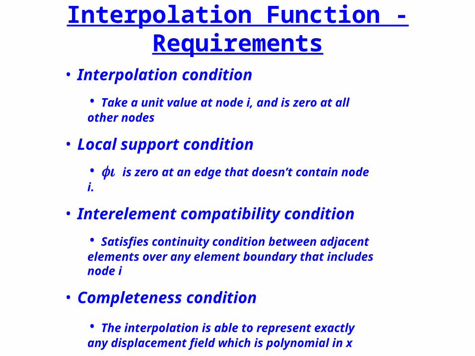
Interpolation Function - Requirements

• Interpolation condition

• Take a unit value at node i, and is zero at all other nodes

• Local support condition

• is zero at an edge that doesn’t contain node i.

• Interelement compatibility condition

• Satisfies continuity condition between adjacent elements over any element boundary that includes node i

• Completeness condition

• The interpolation is able to represent exactly any displacement field which is polynomial in x and y with the

order of the interpolation function

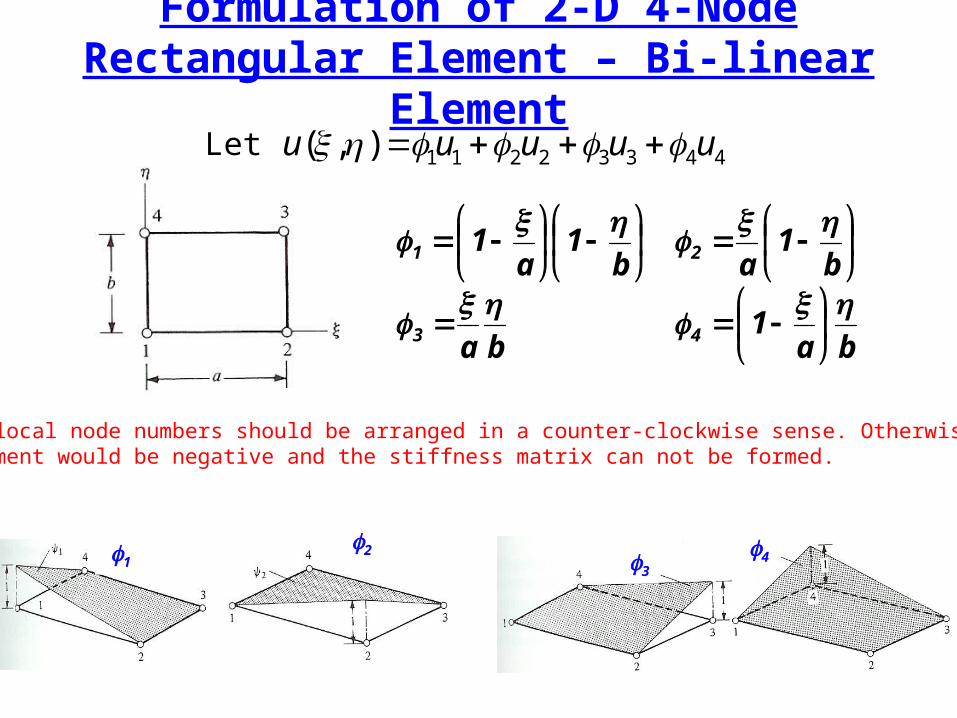
Formulation of 2-D 4-Node Rectangular Element – Bi-linear Element

1 1 2 2 3 3 4 4( , )u u u u u

ba1

ba

b1

ab1

a1

43

21

1 2

3

4

Note: The local node numbers should be arranged in a counter-clockwise sense. Otherwise, the area Of the element would be negative and the stiffness matrix can not be formed.

Let

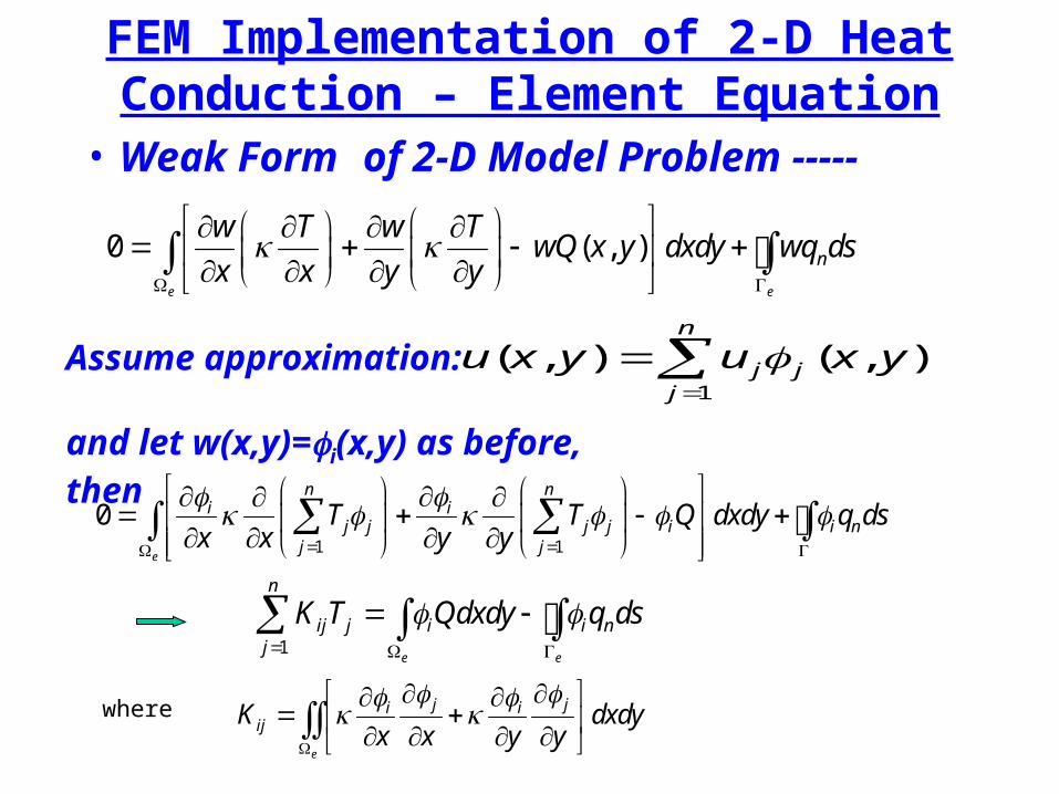
• Weak Form of 2-D Model Problem -----

Assume approximation:

and let w(x,y)=i(x,y) as before, then

1

( , ) ( , )n

j jj

u x y u x y

1 1

0e

n ni i

j j j j i i nj j

T T Q dxdy q dsx x y y

0 ( , )e e

n

w T w TwQ x y dxdy wq ds

x x y y

1e e

n

ij j i i nj

K T Qdxdy q ds

e

j ji iijK dxdy

x x y y

where

FEM Implementation of 2-D Heat Conduction – Element Equation

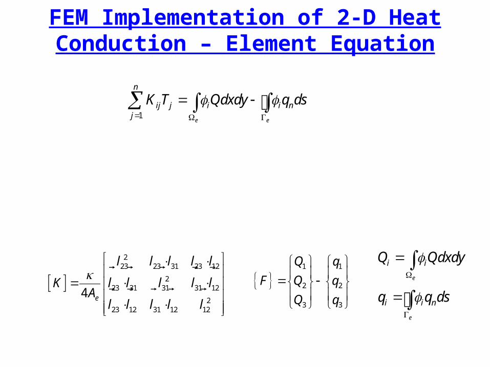
1e e

n

ij j i i nj

K T Qdxdy q ds

223 23 31 23 12

223 31 31 31 12

223 12 31 12 12

4 e

l l l l l

K l l l l lAl l l l l

FEM Implementation of 2-D Heat Conduction – Element Equation

1 1

2 2

3 3

Q q

F Q q

Q q

e

e

i i

i i n

Q Qdxdy

q q ds

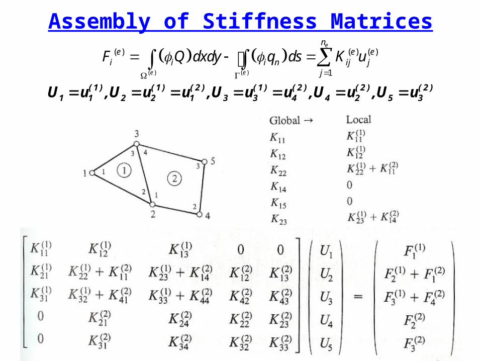
Assembly of Stiffness Matrices

)2(35

)2(24

)2(4

)1(33

)2(1

)1(22

)1(11 uU,uU,uuU,uuU,uU

( ) ( )

( ) ( ) ( )

1

e

e e

ne e ei i i n ij j

j

F Q dxdy q ds K u

Imposing Boundary Conditions

The meaning of qi:

(1) (1) (1)1 12 23 31

(1) (1)12 23

(1) (1) (1) (1) (1) (1) (1) (1) (1)2 2 2 2 2

(1) (1) (1) (1)2 2

n n n n

h h h

n n

h h

q q ds q ds q ds q ds

q ds q ds

(1) (1) (1)1 12 23 31

(1) (1)23 31

(1) (1) (1) (1) (1) (1) (1) (1) (1)3 3 3 3 3

(1) (1) (1) (1)3 3

n n n n

h h h

n n

h h

q q ds q ds q ds q ds

q ds q ds

(1) (1) (1)1 12 23 31

(1) (1)12 31

(1) (1) (1) (1) (1) (1) (1) (1) (1)1 1 1 1 1

(1) (1) (1) (1)1 1

n n n n

h h h

n n

h h

q q ds q ds q ds q ds

q ds q ds

1

2

3

11

2

3

1

2

3

11

2

3

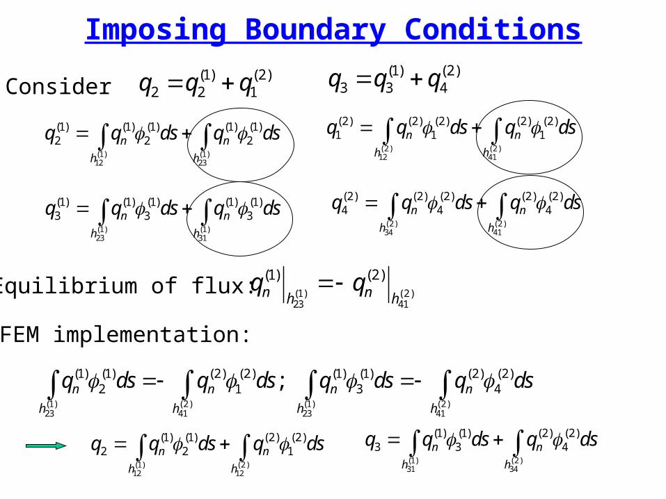
Imposing Boundary Conditions

(1) ( 2)23 41

(1) (2)n nh hq qEquilibrium of flux:

(1) ( 2) (1) ( 2)23 41 23 41

(1) (1) (2) (2) (1) (1) (2) (2)2 1 3 4; n n n n

h h h h

q ds q ds q ds q ds

FEM implementation:

(1) (2)2 2 1q q q

(1) (1)12 23

(1) (1) (1) (1) (1)2 2 2n n

h h

q q ds q ds

Consider

( 2) ( 2)12 41

(2) (2) (2) (2) (2)1 1 1n n

h h

q q ds q ds

(1) ( 2)12 12

(1) (1) (2) (2)2 2 1n n

h h

q q ds q ds (1) ( 2)31 34

(1) (1) (2) (2)3 3 4n n

h h

q q ds q ds

(1) (2)3 3 4q q q

(1) (1)23 31

(1) (1) (1) (1) (1)3 3 3n n

h h

q q ds q ds ( 2) ( 2)34 41

(2) (2) (2) (2) (2)4 4 4n n

h h

q q ds q ds

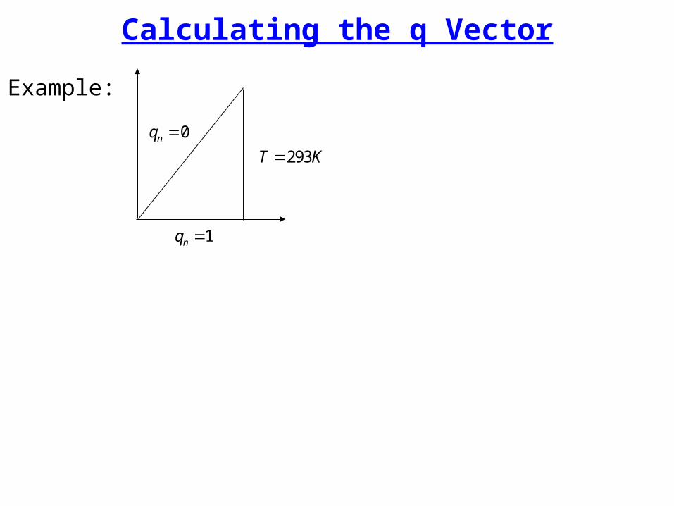
Calculating the q Vector

Example:

293T K0nq

1nq

2-D Steady-State Heat Conduction - Example

0nq

0.6 m

0.4 m

A

BC

DAB and BC:

CD: convectionCm

Wh o 250 CT o25

DA: CT o180

x

y