MDOT STATE STUDY #269 - Driven Pile Load Test Data

MDOT STATE STUDY #269 - Driven Pile Load Test Data Analysis and Calibration of LRFD Resistance Factor for Mississippi Soils

A Final Report Submitted by:

Eric J. Steward, Ph. D., P.E. Associate Professor, Department of Civil, Coastal, & Environmental Engineering

University of South Alabama Mobile, AL 36688

[email protected] 251-460-6174

Co-Authored by Graduate Students: Axel Arnold Yarahuaman Chamorro Dianabel Jackeline Giron Gonzalez

December 2020

ii

FHWA Technical Report Documentation Page 1. Report No. FHWA/MDOT-RD-20-269

2. Government Accession No.

3. Recipient’s Catalog No.

4. Title and Subtitle Driven pile load test data analysis and calibration of LRFD Resistance factor for Mississippi soils

5. Report Date December 22, 2020 6. Performing Organization Code

7. Author(s) Eric Steward, Ph.D. PE (ORCID: 0000-0002-1714-740X) Dianabel Giron Gonzalez Axel Yarahuaman

8. Performing Organization Report

9. Performing Organization Name and Address University of South Alabama Department of Civil, Coastal, & Environmental Engineering 150 Student Services Drive Mobile, AL 36688

10. Work Unit No. (TRAIS) 11. Contract or Grant No.

12. Sponsoring Agency Name and Address Mississippi Department of Transportation Research Division 86-01 PO Box 1850 Jacksion, MS 39215-1850

13. Type Report and Period Covered January 2017 to December 2020 14. Sponsoring Agency Code

15. Supplementary Notes

16. Abstract The Mississippi Department of Transportation (MDOT) currently uses LRFD. However, the LRFD resistance factor used does not necessarily represent the Mississippi soils. A pair of authors have already calibrated LRFD resistance factors for other states using First Order Second Moment (FOSM). However, FOSM leads to over-conservatism. Thus, this study calibrated LRFD resistance factors using the First Order Reliability Method and Monte Carlo Simulation (MCS) rather than FOSM. MCS was found to be the most efficient method. Moreover, pile setup factors were obtained in different sets of data. Finally, the calibrated resistance factors were compared with the recommended resistance factors from published studies from the federal government and the state of Alabama in terms of accuracy. The resistance factors generated in this study are recommended for use based on MDOT’s design methodology. 17. Key Words Pile Design, LRFD, Pile Setup

18. Distribution Statement

19. Security Classif. (of this report) Unclassified

20. Security Classif. (of this page) Unclassified

21. No. of Pages 73

22. Price

iii

DISCLAIMER

The University of South Alabama and the Mississippi Department of Transportation do not

endorse service providers, products, or manufacturers. Trade names or manufacturers’ names

appear herein solely because they are considered essential to the purpose of this report.

The contents of this report do not necessarily reflect the views and policies of the sponsor

agency.

iv

MDOT – STATEMENT OF NONDISCRIMINATION

The Mississippi Department of Transportation (MDOT) operates its programs and services

without regard to race, color, national origin, sex, age or disability in accordance with Title VI of

the Civil Rights Act of 1964, as amended and related statutes and implementing authorities.

MISSION STATEMENTS

The Mississippi Department of Transportation (MDOT)

MDOT is responsible for providing a safe intermodal transportation network that is planned,

designed, constructed and maintained in an effective, cost efficient and environmentally sensitive

manner.

The Research Division

MDOT Research Division supports MDOT’s mission by administering Mississippi’s State

Planning and Research (SP&R) Part II funds in an innovative, ethical, accountable, and efficient

manner, including selecting and monitoring research projects that solve agency problems, move

MDOT forward, and improve the network for the traveling public.

v

AUTHOR ACKNOWLEDGMENTS

The authors wish to thank to the Mississippi Department of Transportation for sponsoring this

research, especially, Sean Ferguson and Michael Stroud in the Geotechnical Engineering

department.

vi

TABLE OF CONTENTS

Page

LIST OF TABLES ........................................................................................................... viii

LIST OF FIGURES ............................................................................................................ x

LIST OF ABBREVIATIONS ........................................................................................... xii

EXECUTIVE SUMMARY .............................................................................................. xiv

– INTRODUCTION ...................................................................................... 1

– LITERATURE REVIEW .......................................................................... 4

2.1 Driven Piles ..................................................................................................... 4 2.2 Basic Pile Design ............................................................................................ 5

2.2.1 Software Program Analysis .................................................................. 5

2.2.2 APile ..................................................................................................... 6

2.3 Allowable Stress Design (ASD) Method ........................................................ 7 2.4 Load and Resistance Factor Design (LRFD) Method ..................................... 8 2.5 Pile Axial Load Test ..................................................................................... 11

2.5.1 Static Load Test .................................................................................. 11

2.5.2 Dynamic Load Test ............................................................................. 14

2.6 Pile Setup ...................................................................................................... 17 2.7 Research Purpose .......................................................................................... 18

– RESEARCH DATABASE AND METHODOLOGY .......................... 20

3.1 Research Database ........................................................................................ 20 3.2 Database Organization .................................................................................. 22 3.3 Driven Piles Database – Load Testing Data ................................................. 23 3.4 Calibration Methodology .............................................................................. 29

3.4.1 Random Variables and Bias ................................................................ 29

3.4.2 Mean, Standard deviation, and Coefficient of Variation of random

variables. ...................................................................................................... 30

3.4.3 FOSM calibration concept and procedure. ......................................... 31

3.4.4 FORM Calibration concept and procedure. ........................................ 32

vii

3.4.5 Monte Carlo simulation concept and procedure ................................. 39

3.5 Reliability Based Efficiency Factor .............................................................. 42 3.6 LFRD Resistance Factors Calibration .......................................................... 44

3.6.1 Target Reliability Index ...................................................................... 44

3.6.2 Dead and Live loads characterization ................................................. 44

- RESEARCH FINDINGS ....................................................................... 46

4.1 Preliminary Resistance Factors ..................................................................... 46 4.2 Estimating Pile Setup Factors ....................................................................... 53 4.3 Comparison of Resistance Factors. ............................................................... 57

4.3.1 Comparison of Resistance Factor results with AASHTO. ................. 58

4.3.2 Comparison of Resistance Factors with NCHRP 507 ........................ 59

4.3.3 Comparison of Resistance Factors with the State of Alabama. .......... 62

4.3.4 Summary of MDOT Resistance Factors compared to AASHTO,

NCHRP 507, and the State of Alabama. ...................................................... 63

- CONCLUSIONS ..................................................................................... 65

– RECOMMENDATIONS ....................................................................... 67

REFERENCES .................................................................................................................. 68

viii

LIST OF TABLES

Page

Table 1. Summary of Computer Analysis Software for Axial Single Pile Analysis (FHWA,

2016). .................................................................................................................................. 5

Table 2: List of the nine soil profiles encountered at each pile location .......................... 23

Table 3: Number of piles categorized by the pile material and soils encountered .......... 23

Table 4: Detailed Set of Data for Case A ........................................................................... 24

Table 5: Detailed Data Set for Case B ............................................................................... 24

Table 6: Detailed Data Set for Case C ............................................................................... 25

Table 7: Detailed Data Set for Case D ............................................................................... 26

Table 8: Reliability index values based on pile groups ..................................................... 44

Table 9: Load statistical values used. ................................................................................ 44

Table 10: Preliminary resistance factors for Data Case A ................................................. 46

Table 11: Preliminary resistance factors for Data Case B ................................................. 47

Table 12: Preliminary resistance factors for Data Case C ................................................. 48

Table 13: Preliminary resistance factors for Data Case D ................................................. 50

Table 14: Summary of average results for piles setup factor with time after EOID greater

than a day based on pile material type. ........................................................................... 54


than a day based on soil profile. ....................................................................................... 54


than a day based on soil region. ....................................................................................... 56

Table 17: Comparison of the MDOT resistance factors with AASHTO specifications. ..... 58

Table 18: Comparison of the resistance factors from MDOT with the resistance factors

from NCHRP 507 (PSC). ..................................................................................................... 60


from NCHRP 507 (HP). ...................................................................................................... 60

ix


from NCHRP 507 (SPP). ..................................................................................................... 61


from the state of Alabama. ............................................................................................... 62

Table 22: Recommended resistance factors for driven piles in the state of Mississippi . 66

x

LIST OF FIGURES

Page

Figure 1: Probability density function for load and resistance when ASD is used (Cleary,

2019). .................................................................................................................................. 8

Figure 2: Probability density function for load and resistance when LRFD is used

(Cleary, 2019). .................................................................................................................. 10

Figure 3: Static load test diagram (FHWA, 2016) .............................................................. 12

Figure 4: Load‐Displacement Curve and The Davisson offset method (Hannigan et al,

2016) ................................................................................................................................. 13

Figure 5: Typical setup of devices and gauges during dynamic testing (ASTM D4945‐08)

........................................................................................................................................... 15

Figure 6: Wave propagation in a pile (Hannigan et al, 2016). .......................................... 15

Figure 7: Location and type of piles used in this study in the State of Mississippi .......... 21

Figure 8: Geologic map of the state of Mississippi (Mississippi Mineral Resources

Institute). ........................................................................................................................... 28

Figure 9: Schematic representation of a random variable as a function (Nowak and

Collins, 2013). .................................................................................................................... 29

Figure 10: Iteration procedure flowchart from Step 9. .................................................... 38

Figure 11: Illustration of the efficiency factor as a measure of the effectiveness of a

design method when using resistance factors (Paikowsly et al, 2004) ............................ 43

Figure 12: FOSM vs FORM results, Case A. ....................................................................... 52

Figure 13: FOSM vs MCS results, Case A. ...................................................................... 52

Figure 14: FORM vs MCS results, Case A. ......................................................................... 53

Figure 15: Setup factor average results according to pile type. ....................................... 55

Figure 16: Setup factor average results according to soil category. ................................. 55

Figure 17: Setup factor average results according to soil region. .................................... 57

Figure 18: Static analysis methods with the highest resistance factors for redundant

piles. .................................................................................................................................. 63

xi

Figure 19: Static analysis methods with the highest resistance factors for non‐redundant

piles. .................................................................................................................................. 64

xii

LIST OF ABBREVIATIONS

COVQ Coefficient of variation of loads or coefficient of variation of the bias values for

the loads.

COVQD Coefficient of variation of dead load or coefficient of variation of the bias values

for the dead load.

COVQL Coefficient of variation of live load or coefficient of variation of the bias values

for the live load.

COVR Coefficient of variation of the resistance or coefficient of variation of the bias

values for the resistance.

G Limit state equation function

gi Limit state function of value i

n Number of failures

N Number of simulations for Monte Carlo simulation.

NORMSINV A Microsoft Excel function that returns the inverse of the standard normal

distribution.

Pf true True probability of failure

Pf: Probability of failure

q* Trial Load standard normal space design point

Q Load random variable

q Standard normal space design point for the load

qD Predicted (nominal) value of dead load.

QDi, λQD,i Simulated dead load value i

Qi, λQ,I Simulated load value i

qL Predicted (nominal) value of live load.

QLi, λQL,I Simulated live load value i

Qn Nominal load.

r* Trial Resistance standard normal space design point

R Resistance random variable

r Standard normal space design point for the resistance.

REOID Nominal EOID resistance.

xiii

Ri, λR,I Simulated resistance value i

rn, Rn Nominal resistance

Rsetup Nominal setup resistance increase

Vp Coefficient of variation of the estimated probability established

β Reliability index

βT Target reliability index.

γavg Average load factor

γQ Load factor for loads.

γQD Load factor for dead load.

γQL Load factor for live load.

η Dead-to-live ratio (QD/QL)

λQ Normal mean of the bias values for the loads.

λQD Normal mean of the bias values for the dead load.

λQL Normal mean of the bias values for the live load.

λR Normal mean of the bias values for the resistance.

σQ Standard deviation for the load Q or the measured load Qmeasured.

σQN The normal standard deviation for the load Q.

σR Standard deviation for the resistance R or the measured resistance Rmeasured.

σλD Standard deviation of the dead load dataset.

σλL Standard deviation of the live load dataset.

σλR Standard deviation of the resistance dataset.

фEOID Resistance Factor for EOID nominal resistance

фR,ф Resistance Factor

фR/λ Bias Efficiency factor

фsetup Resistance Factor for setup nominal resistance.

xiv

EXECUTIVE SUMMARY

In 2007, the American Association of State Highway and Transportation Officials

(AASHTO) published a new policy requiring the application of the Load and Resistance Factor

Design (LRFD) methodology for pile foundations. The Mississippi Department of

Transportation (MDOT) currently uses LRFD. However, the LRFD resistance factor used does

not necessarily represent the Mississippi soils. A pair of authors have already calibrated LRFD

resistance factors for other states using First Order Second Moment (FOSM). However, FOSM

leads to over-conservatism. Thus, this study calibrated LRFD resistance factors using the First

Order Reliability Method and Monte Carlo Simulation (MCS) rather than FOSM. MCS was

found to be the most efficient method. Moreover, pile setup factors were obtained in different

sets of data. Finally, the calibrated resistance factors were compared with the recommended

resistance factors from published studies from the federal government and the state of Alabama

in terms of accuracy. The resistance factors generated in this study are recommended for use

based on MDOT’s design methodology.

1

– INTRODUCTION

Pile foundations are used extensively as support for high-rise buildings, bridges and other

heavy structures, and to safely transfer the structural loads and moments to the ground. Piles are

also used to avoid excess settlement or lateral movement. Piles are designed to carry the

structural loads and maintain construction costs as low as possible at the same time.

Nevertheless, the design of pile foundations involves a significant number of uncertainties which

can be translated generally to over-conservatism. One way to decrease the construction costs is

to develop more accurate prediction methods through static analysis methods, design programs,

dynamic analysis methods, and pile setup consideration. If the anticipated pile resistance is more

accurately estimated before driving, pile lengths and sizes can be reduced and, hence, cost

savings are achieved. Therefore, it is clear that managing uncertainty is largely important to use

resources, time, and money efficiently.

The basic pile design starts with static analysis methods or design programs. Both are

related since design programs incorporate one or more static analysis methods to estimate the

pile capacity. The static analysis methods allow engineers to estimate the pile length and pile size

prior to installation. Several static analysis methods are available and each one of them has

specific applications, limitations, and soil parameters required. In the same way, several design

programs have become more popular due to their time efficiency, and they use these static

analysis methods to determine the estimate capacity of the pile at specific locations. These

programs include DrivenPile and APile, which are available commercially.

Once the pile length, pile size, and nominal resistance are estimated through static

analysis methods or design programs, the designs are confirmed during construction by field

control determination tests or methods. The most accurate method to verify the pile capacity is

through static load testing. Static load tests consist of loading the pile using a load cell attached

to a reaction system that keeps the load cell fixed. The load increases gradually until failure.

Another method used to verify or revise design is through dynamic load testing based on

dynamic analysis and wave propagation theory. Dynamic tests consist of a hammer hitting the

head of a pile during and after installation. The compression wave data during hammer blows is

obtained and processed through a Pile Driving Analyzer (PDA), which can incorporate signal

2

matching (CAPWAP). Dynamic load testing can be considered as an economically efficient

method to determine the capacity of a pile compared to the significant cost of static load testing.

Another aspect of design capable of producing cost-savings for pile design is the

phenomenon known as pile setup, which consists of a pile resistance or capacity increase over

some time interval after installation. When the pile is being driven, the surrounding soil is

disturbed and loses strength. Once the installation has finished, the same soil starts a process to

attempt to recover lost strength, which contributes to an increase in the pile capacity. If the pile

capacity increase is accurately anticipated, the pile length, sizes and quantity can be decreased,

hence lower costs would be required. Pile setup capacity increase can be measured immediately

or some time interval after installation through dynamic load tests. Several prediction models to

predict this capacity increase are available, but the most popular is the Skov and Denver [1]

model.

Driven piles have been designed following the Allowable Stress Design (ASD)

methodology for years. ASD represents the construction uncertainties and safety margin

typically through a single factor of safety (FS). For ASD, the pile capacity is reduced by dividing

the nominal pile capacity by the FS. Nonetheless, the limitations of ASD were recognized in the

1990s [2]. Consequently, an alternative design methodology known as Load and Resistance

Factor Design (LRFD) has been developed since the mid-1980 [3] and is becoming more popular

due its reliability basis. For LRFD, loads and resistance have different sources and levels of

uncertainty. Thus, each one (loads and resistances) is modified by partial factors. The loads are

affected by load factors that are larger or equal to 1. The resistance is affected by resistance

factors that are smaller or equal to 1. In other words, if LRFD is employed, the loads are

amplified while the resistance is underestimated. In this way, LRFD generates a design with

more consistency and uniform level of safety [2]. Consequently, more economically efficient and

repeatable designs are possible compared to ASD methodology [3].

Under LRFD, the resistance is reduced by multiplying the nominal capacity by a

resistance factor (ф). This resistance factor can be lower or equal to 1 and can be calibrated for a

specified regional soil if enough statistical data is available. The calibration depends on

significant data sizes and is based on probability theory. The most widely used probability-based

methods to calibrate a resistance factor are the First Order Second Method (FOSM), the First

Order Reliability Method (FORM), and Monte Carlo Simulation (MCS). The three methods

3

require a resistance bias factor (λR) obtained from the ratio between a set of measured capacity

data and a set of predicted capacity data. The measured capacity is obtained from field test such

as dynamic and static load testing, while the predicted capacity is obtained from static analysis

method or design programs.

Overthe past few decades, several efforts have been made to implement and develop

LRFD resistance factors for deep foundations for bridges. Nonetheless, the transition has been

relatively slow [4] due to the large quantity and quality of data required, as well as deficiencies

included in the early development of LRFD specifications. The American Association of State

Highway and Transportation Officials (AASHTO) and the Federal Highway Administration

(FHWA) published a policy that turned into an obligation for the usage of LRFD for all new

bridges initiated after October 1st, 2007. Therefore, AASHTO also provided some recommended

resistance factors for various design methods along with the policy. Nevertheless, several

Departments of Transportation (DOTs) expressed their concern about the accuracy and over-

conservatism of these resistance factors when applied to specific regions [3]. Consequently,

AASHTO and FHWA allowed the state Department of Transportations to develop their

regionally calibrated LRFD resistance factors for bridge foundations incorporating statistical and

reliability theory using existing databases. Since then, several DOTs started working on the

composition of adequate databases and the development of their own LRFD resistance factors to

eliminate over-conservative designs and generate cost savings to the state and taxpayers.

Studies conducted by NCHRP 507 [5], Styler [6], Haque and Abu-Farsakh [7] revealed

that FOSM tends to lead to some over-conservatism. For instance, NCHRP 507 [5] found that

FOSM provides resistance factors 10% lower than FORM. Moreover, Styler [6] contends that

FORM resistance factors tend to be 8%-23% larger than FOSM resistance factors. Also, Allen et

al. [8] suggests that MCS is more adaptable and rigorous method than FOSM and provides

resistance factors consistent with FORM. Consequently, the main objective of this study is to

develop LRFD resistance factors unique to Mississippi soils using FOSM, FORM, and MCS, in

order to enhance accuracy and efficiency of pile design. The second objective is to develop pile

setup factors in different sets of data. Finally, the third objective is to compare the calibrated

resistance factors with the recommended resistance factors from published studies.

4

– LITERATURE REVIEW

This chapter describes and explains the basic concepts and background information

applied to the subsequent chapters of this study. The main conceptual sections included are (1)

driven piles, (2) basic pile design, (3) ASD methodology, (4) LRFD methodology, (5) pile load

testing, and (6) pile setup. Some sentences, tables, figures, graphs, and equations will be

referenced in the following chapters of the study.

2.1 Driven Piles

The first problem for a foundation designer is to establish whether the soil conditions are

suitable to support the structure using shallow foundations or deep foundations (such us piles).

Vesic [9] says that “piles are used where upper soil strata are compressible or weak; where

footings cannot transmit inclined, horizontal, or uplift forces; where scour is likely to occur;

where future excavation may be adjacent to the structure; and where expansive collapsible soils

extend for a considerable depth”. The FHWA [10] adds that pile foundations are used

extensively to support buildings, bridges, and other heavy structures, to safely transfer structural

loads to the ground, and to avoid excess settlement or lateral movement. According to Pement

[2], driven piles and drilled shaft are the most common deep foundations.

Driven piles can be installed by impact driving or vibrating. There are two types of driven

piles: End-bearing piles and friction piles. On one hand, End-bearing piles resist loads through

the interaction of the cross-sectional area of its tip and the hard layer beneath. Although a

minimal friction resistance is developed, this is usually ignored. On the other hand, friction piles

resist loads through the interaction and friction of the perimetrical pile area and the soil around it.

When bedrock is not encountered at a reasonable depth below the ground surface, piles can resist

loads through both end-bearing and frictional resistance for economic efficiency [2].

5

2.2 Basic Pile Design

One of the most important challenges for foundation engineering, especially for pile

design, is to develop a safe and cost-effective foundation system. National committees such as

the FHWA, American Concrete Institute (ACI), American Institute of Steel Construction

(AISC), and the AASHTO are deeply involved in the updating of design requirements. However,

in the geotechnical field, several variables affect the soil conditions and its interaction with a

structure. Therefore, the soil conditions can be estimated, but cannot be determined with

complete accuracy [2]. Generally, the required capacity and depth shall be estimated before

driving the pile. Thus, it is vital to predict the amount of nominal resistance of the pile with a

reasonable accuracy despite the complex nature of the soils. This prediction or design can be

performed through static analysis or design programs, which can implement several design

methods.

2.2.1 Software Program Analysis

Due to its time efficiency, software program analysis is becoming more popular for

engineering purposes. As indicated by Pement [2], Software Program Analysis are mainly used

for axial loaded single piles or pile groups. These programs can include one or several static

analysis design methods. Also, they incorporate different soil layers, soil types, soil

characteristics, which are used to estimate the pile capacity according to a specific depth. Table 1

summarizes some of the available commercial programs including the static analysis programs

that they are based on.

Table 1. Summary of Computer Analysis Software for Axial Single Pile Analysis (FHWA, 2016).

Computer Program

Static Analysis Methods In Program

Method Presented in GEC-12 (2016)

Method Presented in AASHTO 7th edition (2014)

AllPile Navfac DM-7 No No A-Pile API-RP2A Yes No A-Pile US Army COE No No

6

A-Pile FHWA (Alpha / Nordlund) Yes Yes A-Pile Lambda Method No Yes A-Pile NGI (CPT) No No A-Pile ICP (CPT) No No DrivenPiles Alpha Method Yes Yes DrivenPiles Nordlund Method Yes Yes FB-Deep FDOT SPT Method No No FB-Deep Schmertmann (CPT) Yes Yes FB-Deep UF (CPT) No No FB-Deep LCPC (CPT) No No Unipile Alpha Method Yes Yes Unipile Beta Method Yes Yes, but differs Unipile Elsame and Fellenious (CPT) Yes No Unipile Schmertmann (CPT) Yes Yes Unipile LCPC (CPT) No No Unipile Meyerhof (SPT) No Yes

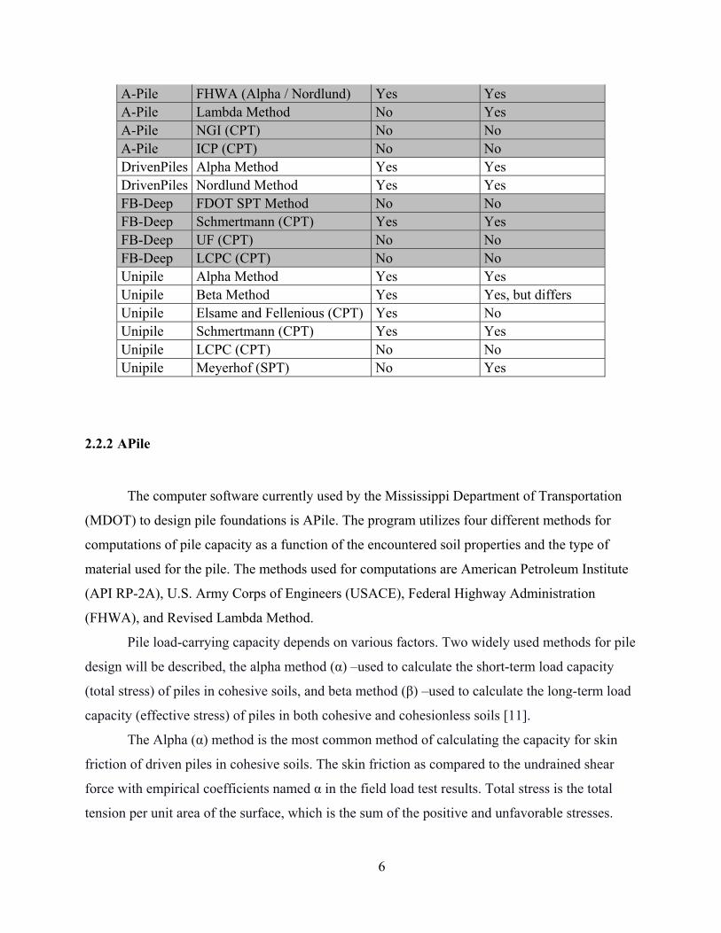
2.2.2 APile

The computer software currently used by the Mississippi Department of Transportation

(MDOT) to design pile foundations is APile. The program utilizes four different methods for

computations of pile capacity as a function of the encountered soil properties and the type of

material used for the pile. The methods used for computations are American Petroleum Institute

(API RP-2A), U.S. Army Corps of Engineers (USACE), Federal Highway Administration

(FHWA), and Revised Lambda Method.

Pile load-carrying capacity depends on various factors. Two widely used methods for pile

design will be described, the alpha method (α) –used to calculate the short-term load capacity

(total stress) of piles in cohesive soils, and beta method (β) –used to calculate the long-term load

capacity (effective stress) of piles in both cohesive and cohesionless soils [11].

The Alpha (α) method is the most common method of calculating the capacity for skin

friction of driven piles in cohesive soils. The skin friction as compared to the undrained shear

force with empirical coefficients named α in the field load test results. Total stress is the total

tension per unit area of the surface, which is the sum of the positive and unfavorable stresses.

7

The beta method (β) allows the engineer to calculate the vertical bearing capacity of a

separate pile in both cohesive and non-cohesive soils. By obtaining total stress and pore water

pressures information, effective stress can be measure. The method is based on effective stress

analysis and is suited for long-term (drained) analyses of pile load capacity [11]. Also, regular

stresses and just not shear stresses are defined by the concept of effective stress. Soil deformation

is a vital stress mechanism, not an overall tension.

2.3 Allowable Stress Design (ASD) Method

ASD design methodology has been used for decades in the Geotechnical engineering

field as a way to incorporate uncertainties into a design. This method consists of utilizing a limit

equilibrium analysis by keeping the anticipated loads lower than the capacity or resistances. In

ASD, the uncertainties in the loads and resistances are expressed in an incorporated value named

“Factor of Safety” (FS). Pement [2] suggests that the uncertainties from a design method are

most likely due to (1) variability of engineering properties and load predictions, (2) errors in

measuring material resistance, (3) errors in prediction models used, and (4) sufficiency and

applicability of sampling and testing methods. The ASD design equation used is the following:

𝑅𝐹𝑆

𝑄 (1)

where Rn is the nominal resistance (capacity), FS is the Factor of Safety, and ∑ 𝑄 is the sum of

load effects (dead, live, and environmental) applied on a pile [12].

Nevertheless, ASD is becoming less popular due to the following limitations. (1) The Factor of

Safety (FS) is a subjective value that is not based of probability of failure. The FS just depends

on the design models and material parameters selected [2]. (2) ASD assumes similar

uncertainties for load and resistance variables. (3) ASD is based only on experience and

engineering judgment, which can lead to over conservatism [12]. Even though several sources of

uncertainties can be considered by the designer when using ASD, their consideration is mainly

qualitative rather than quantitative [13].

8

Figure 1 shows the way ASD reduces the probability of failure when probability density

functions are evaluated. Failure is defined as loads exceeding the resistance, which graphically

represented by the area formed by the load curve overlapping the resistance curve. The graph on

the left shows when load and resistance are unmodified, hence, they are similar theoretically.

The graph on the right shows when the resistance has been modified by the FS. The

displacement of the resistance probability density function curve, due to the FS, reduces the

probability of failure by decreasing the overlapped area. The new failure area is represented in

orange color.

Figure 1: Probability density function for load and resistance when ASD is used (Cleary, 2019).

2.4 Load and Resistance Factor Design (LRFD) Method

Load and Resistance Factor Design (LRFD) is an alternative design methodology

specifically and progressively developed for bridges since the mid-1980s [3]. LRFD originated

due to the limitations of ASD methodology recognized in the 1990s [2]. Moreover, AASHTO

required the LRFD method to design deep foundations supporting bridges in 2007. The LRFD

design equation is the following:

9

ф𝑅 𝛾 𝑄 , (2)

where ф is the resistance factor, Rn is the nominal resistance or capacity, γi is the load factor, Qi

is the nominal load value.

Under LRFD, both loads and resistance have different sources and levels of uncertainty. These

uncertainties can be quantified using probability-based procedures to satisfy engineered design

with consistent and specific levels of reliability. Paikowsky et al. [5] says that “The principal

difference between Reliability Based Design and the traditional or partial factors of safety design

approaches lies in the application of reliability theory, which allows uncertainties to be

quantified and manipulated consistently in a manner that is free from self-contradiction.” In other

words, the implementation of LRFD allows the separation of uncertainties from loads and

resistances and, then, to use methods based on probability theory to satisfy a prescribed margin

of safety [5]. It should be noted that since loads are better known than resistances, the load effect

usually has smaller variability than the resistance effect.

Figure 2 shows the way LRFD reduces the probability of failure when probability density

functions are evaluated. Failure is defined as loads exceeding the resistance. This failure is

graphically translated to point where the load curve overlaps the resistance curve. The graph on

the left shows when load and resistance are unmodified, hence, they are similar theoretically.

The graph on the right shows when the loads have been factored (increased) by the load factors

and the resistance has been factored (decreased) by the resistance factor. The displacement of the

load and resistance probability density function curve to opposite directions reduces the

probability of failure by decreasing the overlapped area. The new failure area is represented in

orange color.

10

Figure 2: Probability density function for load and resistance when LRFD is used (Cleary, 2019).

As mentioned by Paikowsky et al [5], some of the specific benefits of implementing

LRFD for pile design include the following:

Cost savings and improved reliability due to more efficiently balanced design.

More rational and rigorous treatment of uncertainties in the design.

Enhanced perspective on the overall design and construction processes.

Development of probability-based design method capable of stimulating advances

in pile analysis and design.

Conversion of the codes into living and easier to revise documents.

The factors of safety previously used provide a framework to extrapolate existing

design procedures into newer foundation concepts and materials.

Currently the Mississippi DOT utilizes LRFD in the design methodology of driving piles

by incorporating the resistance factors developed from the national database as generated by the

AASHTO Design Manual [14]. However, utilizing regionally calibrated resistance factors are

recommended and preferred to increase the accuracy of the predicted capacity of driven piles.

11

2.5 Pile Axial Load Test

Load testing is the most accurate way to determine the nominal capacity of a pile [2].

Due to the high uncertainty of soils involve, it is imperative to perform actual load tests before or

during construction to verify the preliminary design. The load tests are best known as field

control methods. AASHTO states that when nominal axial resistance is determined by using

actual load testing, the uncertainty in the nominal axial resistance is solely due to the reliability

of the field determination method. They are mainly classified into two axial field control

methods: Static Load Test (SLT) and Dynamic Load Test (DLT).

2.5.1 Static Load Test

Load tests are commonly conducted to determine a pile foundations' capability to sustain

working loads while offering the right level of safety. Due to the non-availability of established

procedures of assessing mechanisms of transferring loads between the soil and the piles, load

tests are conducted, usually during the design or construction phase [15]. Static Load Test is the

most accurate method to determine the pile load capacity.

FHWA [16] says that “depending upon the size of the project and other project variables,

static load tests may be performed either during the design stage or construction stage.” Usually,

a SLT is performed inside or close to the site of the final pile installation. Once a pile is installed,

a waiting period is required before the pile can be tested.

The axial Static Load Test is regulated by ASTM D 1143-07 [17]. A system of reaction

beams is attached to the load cell to assure minimum displacement as shown in Figure 3

Generally, the reaction beams are connected to reaction piles. ASTM D 1143-07 [17] mentions

several loading methods. However, the Quick Maintained (QM) Testing Method is the fastest

and most efficient when determining the pile capacity [18]. In this method, the load is applied in

increments of 5% of the anticipated nominal resistance. Load can be incremented until pile

failure. The load gradient shall be composed by at least 20 points before reaching the

geotechnical nominal resistance in order to generate a load-displacement curve [2]. The test shall

not last more than one hour as cited by Hannigan et al [19]. Once the load-displacement curve is

plotted, several determination methods or acceptance criteria can be performed, such as the

12

Davisson Method, the Shape of Curvature Method, the Limited Total Settlement Method, the De

Beer Method, the Chin methods, and the Iowa DOT method. However, the Davisson Method is

the most popular method and works better with QM test data [20].

Figure 3: Static load test diagram (FHWA, 2016)

The Davisson Method is used to determine the load at which the pile fails and is based on

the deformation of the pile head. It also uses a drawn line parallel to the elastic compression line

(base line), which is offset by a specified amount of displacement depending on the pile size

[18]. The parallel line is known as the Offset Limit Line or Davisson Line. According to Figure

4, the point of intersection between the Offset Limit Line and the load-displacement curve is

considered the Nominal Resistance or Failure Load.

13

Figure 4: Load‐Displacement Curve and The Davisson offset method (Hannigan et al, 2016)

The Elastic Deformation Line or Base Line can be plotted considering the following equation:

𝛥 , (3)

where Δ is the elastic movement of the base line, Qva is the applied load, A is the cross sectional

are of the pile, E is the modulus of elasticity of the pile material, and L is the embedded length of

the pile.

In addition, to draw the Offset Limit Line or Davisson Line, the following expression can be

used:

𝑋 0.15 ’ (4)

where X is the offset displacement from the base line (inches), and D is the pile diameter

(inches).

With the application of a static load tester, engineers can obtain and record very reliable

readings at various load intervals while monitoring various independent channels taken from

14

embedded sensors or the traditional pile top measurements [21]. The possibility of automatic

data collection techniques allows engineers to monitor, analyze, and interpret the load test results

in real-time. The method of pile load testing differs from other testing methods, such as dynamic

and rapid load testing. The database used in this research project was obtained from dynamic

tests. The Mississippi Department of Transportation did not perform static load tests in the tested

piles that are used in this study.

2.5.2 Dynamic Load Test

Dynamic Load Testing is an economically efficient method to test a pile because the time

involving the setup of testing equipment is low and simple. Dynamic Load Tests are performed

typically during pile installation and a short time after the end of initial driving (EOID) and

consists of obtaining compression wave data during hammer blows onto the pile head [2].

Basically, when the hammer strikes the top of the pile, a compressed stressed zone travels along

the shaft of the pile at a constant wave speed. The speed depends mainly on the pile material.

When the wave hits the pile toe, its amplitude is reduced by the action of static and dynamic soil

resistance forces. Depending on the magnitude of the soil resistance, the wave will return to the

top of the pile as a tensile (reflective) or compressive (incident) force [19]. Figure 5 shows the

setup of the sensors in the crane and hammer system, while figure 6 shows this procedure of

wave propagation.

15

Figure 5: Typical setup of devices and gauges during dynamic testing (ASTM D4945‐08).

Figure 6: Wave propagation in a pile (Hannigan et al, 2016).

According to FHWA [16], Dynamic Load Tests use measurements of strain and

acceleration taken near the pile head as a pile is driven or restrike with a pile driving hammer.

16

These dynamic measurements can be used to determine the performance of the pile driving

system, calculate pile installation stresses, assess pile integrity, and evaluate the nominal

geotechnical resistance [16]. However, Pement [2] says that when the pile is driven into the soil,

the soil beneath behaves dynamically. Thus, it resists the pile in a dynamic manner.

Consequently, it is not accurate to assume that the Dynamic resistance is equal to the Static

resistance.

As mentioned by Pement [2], to perform a DLT, the pile has usually two or more

transducers and accelerometer attached during pile installation. The gauges are connected to a

computerized device called Pile Driving Analyzer (PDA), which receives the wave and energy

data coming from the pile in real time. The PDA provides force and acceleration data, which is

used to establish force and motion within the pile [2]. FHWA [16] adds that test results shall be

better evaluated using signal matching techniques to determine the relative soil distribution on

the pile and the dynamic soil properties to use in wave equation analyses.

There are several wave equations to determine the pile capacity such as dynamic

formulas, wave equations, Case Pile Wave Analysis Program (CAPWAP), and iCAP. The last

two methods are the most popular since they are programs that incorporate wave equations.

Firstly, CAPWAP adopted the Smith [22] soil-pile model using the wave equation algorithm in

the analysis to perform a signals-matching process with the combination of several analytical

techniques [18]. CAPWAP basically partitions the pile into lumped masses linked with linear

elastic springs and viscous dampers [18]. Second, iCAP is an automated version of CAPWAP

designed to adjust for soil damping. Likins et al [23] mentions that iCAP results match very well

with CAPWAP results for several types of piles and soils encountered.

The two ways to control the pile capacity through dynamic testing are through End of

Initial Driving (EOID) and Beginning of Restrike (BOR). EOID is performed usually

immediately after the pile has been installed and consists of restriking the pile head few times to

get dynamic data. BOR analysis can be performed after one- or several-time intervals after EOID

and requires few restrikes on the pile head as well. BOR is usually necessary when the pile

capacity was not reached at EOID or past BOR tests. Dynamic Load Testing allows a

comparison of EOID resistance and BOR resistance. In this way, setup can be quantified.

In summary, dynamic testing is based on wave propagation principles and uses wave

equations to determine the nominal pile capacity. The most popular methods are CAPWAP and

17

ICAP, which are software that incorporate several wave equations. When static load tests are not

available or performed, dynamic load tests are useful to perform EOID and BOR analysis and so

it is possible to quantify the capacity of the pile at various times during and after the installation

of the pile.

2.6 Pile Setup

Pile setup is defined as the pile capacity increase over time and might generate significant

cost savings. Haque et al [7] defined pile setup as “the increase in axial resistance of driven piles

after end of initial driving (EOID).” According to Haque and Steward [24], the incorporation of

pile setup in the design stage would produce meaningful construction cost savings because the

increase in pile capacity can translate into smaller pile elements or shorter embedment lengths.

Pile setup phenomenon is mainly a product of three mechanisms: (1) Increase of soil effective

stress due to the dissipation of excess pore water pressure, (2) thixotropic effect, and (3) stress

independent increase or “aging” effect.

Firstly, during pile driving, the soil is displaced principally radially along the shaft and

vertically below the toe. In the course of the driving process, the soil surrounding the pile loses

strength due to an excessive increase of pore water pressure and distribution of soil pressure

heavily disturbing the soil [25]. Immediately following EOID, this pore water excess begins to

dissipate similarly to a consolidation process. Over time, the soil around the pile attempts to

recover its original strength, which contributes to an increase in axial resistance of the pile [24].

Second, the phenomenon known was thixotropy also produces a regain of strength of the

disturbed soil [26]. Thirdly, Schmertmann [27] indicates that even after the dissipation of excess

pore water pressure is completed, pile setup can continue due to aging mechanism. Haque and

Steward [24] state that aging effects increases the shear modulus, stiffness, dilatancy, friction

angle of the soil and, also, reduces the soil’s compressibility.

Several empirical models have been developed to predict pile setup behavior. However,

the most popular is the one developed by Skov and Denver [1] due to its simplicity. This model

uses the following equation:

𝑅𝑅

𝐴 𝑙𝑜𝑔𝑡𝑡

1, (5)

18

where Rt is the total pile capacity at time t, Rto is the total pile capacity at reference time to, t is

the time elapsed since end of initial pile driving, to is the initial reference time (usually time at

EOID), and A is the setup parameter (log-linear).

The parameter A depends on the soil type, pile material, pile type, pile size, and pile capacity

[24]. Skov and Denver [1] generally suggests using A = 0.2 for sand and A = 0.6 for clay.

The incorporation of setup into the calibration of LRFD resistance factors has been

studied by Yang and Liang [28] and Haque et al. [7]. They take as basis the limit equation the

same used by AASHTO [14], which does not incorporate setup:

ф 𝑅 𝛾 𝑞 𝛾 𝑞 , (6)

where Rn is the predicted resistance, φR is the resistance factor for Rn, qD and qL are the predicted

dead and live loads, respectively; and γQD and γQL are the load factors for qD and qL, respectively.

In this way, Yang and Liang [28] proposes the setup effect of driven piles in the following

equation:

ф 𝑅 ф 𝑅 𝛾 𝑞 𝛾 𝑞 , (7)

where φEOID and φsetup are the resistance factors for reference resistance at tEOID and setup

resistance, respectively. REOID is the nominal resistance at end of initial driving, and Rsetup is the

nominal setup resistance increase.

Haque and Abu-Farsakh [7] evaluated the resistance factors for setup at time intervals of 30, 45,

60 and 90 days after EOID. Their final recommendation is using a setup resistance factor фsetup

of 0.35 at any time after the 14 days.

2.7 Research Purpose

The current MDOT state of practice for the LRFD design of driven piles is to utilize the

generalized resistance factor (φ) as indicated by the AASHTO design manual [14]. The manual

allows for regionally calibrated resistance factors with the appropriate amount of data gathered

within the region. MDOT has tested thousands of piles over the past few decades, yet do not have

a completed database to perform the necessary statistical analysis to calibrate the resistance factors

for design.

19

Research has shown that driven piles experience up to 200% increase in axial resistance

after installation, yet most design engineers neglect to include the effects of setup due to a lack of

reliability and variable site conditions. Pile setup continues to occur beyond the standard 7 day

restrike or load test time and if this long-term bearing capacity can be implemented into the pile

design, the pile size or embedment depth can be reduced, resulting in considerably lower cost of a

project. MDOT currently does not consider setup as a design parameter within the current state of

practice, other than what the pile load tests indicate when the necessary resistances are not achieved

during driving.

The study will develop a state wide pile load test database to then enable the development of a

regionally calibrated LRFD resistance factor to improve the accuracy of driven pile design. The

database will provide trends of pile setup in certain soil conditions within the state to then be

included within the design parameters to improve the efficiency of the design of foundation

elements of structures supporting MDOT bridges.

20

– RESEARCH DATABASE AND METHODOLOGY

3.1 Research Database

The database used for the statistical evaluation of resistance factors for the design and

construction of driven piles in Mississippi Soils was data obtained from MDOT consisting of

PDA records, CAPWAP analyses, geotechnical reports, and the pile design recommendations. It

was essential to organize the information obtained in an appropriate order that allowed a more

efficient manipulation and evaluation of the database. A spreadsheet was composed of the

information for 674 driven piles driven throughout the state of Mississippi. Figure 7 is a map of

Mississippi with the location of each pile used in this study. The three types of piles driven

within the state, Prestressed Concrete Piles (PSC), Steel H-Piles (HP), and Steel Pipe Piles

(SPP), are shown in the figure as well.

21

Figure 7: Location and type of piles used in this study in the State of Mississippi

22

3.2 Database Organization

It is generally suggested to organize the pile database into categories based on the pile

material, soil type along the shaft, soil type beneath the toe, length, and geological regions. The

piles in the database consisted of 283 PSC, 359 HP, and 22 SPP. Note that this is a total of 664

piles, as the type of material for 10 piles was unknown and the reports were unable to be

obtained.

Geotechnical reports were used to determine the soil profiles encountered by each pile.

The soil profile was simplified from many varying layers to either sand, clay, or mixed soil.

Using the length of pile embedment, each pile was categorized by the type of soil encountered

along the shaft and at the tip. The soil in contact with the pile's shaft was grouped to determine

the majority of soil type providing friction resistance. The soil within the range of 10 feet above

to 4 feet below the pile toe was used to determine the majority soil type providing the end

bearing resistance. The depth of each soil layer type (sand or clay) along the embedment depth

was added together, then taken as a percentage of the total embedment depth to find the majority

soil type along the pile shaft. The majority of soil type was determined by applying a simple

35%-65% rule (See Equation 8). If the percentage of a soil type was greater than or equal to

65%, it was considered the majority, while the other 35% was disregarded. If neither type

reached 65%, the profile stated as consisting of mixed soil.

𝑀𝑖𝑛𝑜𝑟𝑖𝑡𝑦 𝑆𝑜𝑖𝑙 𝑇𝑦𝑝𝑒 35% 𝑀𝑖𝑥𝑒𝑑 𝑆𝑜𝑖𝑙 65% 𝑀𝑎𝑗𝑜𝑟𝑖𝑡𝑦 𝑆𝑜𝑖𝑙 𝑇𝑦𝑝𝑒 (8)

During the categorization of the behavior of the soil within these layers, it was observed

that the silt encountered required additional analysis as some silts provided cohesive behavior

while others did not. The silts with cohesive behavior were assumed to be clay, and cohesionless

silts were assumed to be sand. After the soil profiles were created, each pile was provided a code

number based on all of the possible soil types encountered. The list of soil profile scenarios

between the shaft and tip layers can be seen in Table 2.

23

Table 2: List of the nine soil profiles encountered at each pile location

Soil Profile Code 1 2 3 4 5 6 7 8 9

Soil along the Shaft Clay Clay Clay Mixed Mixed Mixed Sand Sand Sand

Soil at the Toe Clay Mixed Sand Clay Mixed Sand Clay Mixed Sand

After a soil profile was determined and assigned to each pile, the four pile groups based

on the material type previously presented were separated by their soil profile type. Each group

was composed of nine subgroups, which is the soil profile code assigned. The number of piles in

each subgroup is presented in Table 3. Soil profile code 9, which indicates the pile encounters

mostly sand throughout its embedment length, is the most common soil type encountered. Note

that 80 piles do not have a soil profile code assigned because there were no geotechnical reports

provided, and 9 piles do not have material type information.

Table 3: Number of piles categorized by the pile material and soils encountered

Pile Material Type Soil Profile Code

Total 1 2 3 4 5 6 7 8 9

ALL 593 106 19 45 54 31 116 20 12 190

PSC 242 41 5 26 25 17 48 8 9 63

HP 321 65 14 18 25 9 63 11 2 114

SPP 21 0 0 0 4 2 2 1 0 12

3.3 Driven Piles Database – Load Testing Data

The number of piles used for the statistical evaluation of resistance factors for the design

and construction of driven piles in Mississippi Soils is different from the initial number of piles

from the primary database due to missing information. Four different sets of data, shown in

Tables 4, through 7, were used in the calibration of the resistance factors based on the level of

detailed information utilized. Case A utilizes all piles only distinguished by the type of pile and

the load test method. Case B only considers the soil profile code of each pile. Case C considered

24

the pile material first and then separated the database of each material into nine subgroups based

on the soil profile code. While Case D considered five different subgroups based on a geologic

map of Mississippi. Figure 8 is the geologic map that was used to categorize the different

subgroups presented in Case D.

Table 4: Detailed Set of Data for Case A

Prediction Method

Measured Method

Data set A Number of

Piles

APILE CAPWAP

All Piles 648 PSC 279 HP 347 SPP 22

APILE PDA

All Piles 652 PSC 280 HP 350 SPP 22

Table 5: Detailed Data Set for Case B

Prediction Method

Measured Method

Data set B Number of

Piles Shaft - Toe Soil Profile

Code

APILE CAPWAP

Clay - Clay 1 101 Clay - Mixed 2 19 Clay - Sand 3 44

Mixed - Clay 4 53 Mixed - Mixed 5 28 Mixed - Sand 6 109 Sand - Clay 7 20

Sand - Mixed 8 11

Sand - Sand 9 183

APILE PDA

Clay - Clay 1 106

Clay - Mixed 2 19

Clay - Sand 3 44

Mixed - Clay 4 53

Mixed - Mixed 5 28

Mixed - Sand 6 108

Sand - Clay 7 20

Sand - Mixed 8 11

25

Sand - Sand 9 183

Table 6: Detailed Data Set for Case C

Prediction Method

Measured Method

Data set C Number of

Piles Material Type

Shaft - Toe Soil

Profile Code

APILE CAPWAP

PSC



Sand - Mixed 8 9 Sand - Sand 9 60

HP




SPP

Mixed - Clay 4 4 Mixed - Mixed 5 2 Mixed - Sand 6 2 Sand - Sand 9 12

APILE PDA PSC




HP Clay - Clay 1 65

26

Clay - Mixed 2 14 Clay - Sand 3 18



SPP

Mixed - Clay 4 4 Mixed - Mixed 5 2 Mixed - Sand 6 2 Sand - Sand 9 12

Table 7: Detailed Data Set for Case D

Prediction Method

Measured Method

Soil Regions Number of

Piles

APILE CAPWAP

Quaternary 191

Tertiary All 336

Tertiary, Soil profile codes: 1-4-

7 130

Tertiary, Soil profile codes: 3-6-

9 150

Cretaceous 38

27

APILE PDA

Quaternary 192

Tertiary All 339

Tertiary Soil profile codes: 1-4-

7 134

Tertiary Soil profile codes: 3-6-

9 149

Cretaceous 38

28

Figure 8: Geologic map of the state of Mississippi (Mississippi Mineral Resources Institute).

29

3.4 Calibration Methodology

This section describes the concepts and probabilistic-based methodologies applied to a

LRFD calibration. These methodologies are based on random variables and the statistical

characterization of their bias values. This section also explains how to conduct an actual

calibration and apply it to the development of LRFD design specifications. Also, the First Order

Second Moment (FOSM) calibration, the First Order Reliability Method (FORM) calibration,

and the Monte Carlo Simulation (MCS) calibration concepts and procedures are explained.

3.4.1 Random Variables and Bias

This section defines the concept of random variables and bias, which both compose the

basis to perform the LRFD calibration. First of all, Allen et al. [8] define a random variable as a

variable that does not have an exact value and it pertains to a set of values, or a range, and the

probability of occurrence. Nowak and Collins [29], add that a random variable is a function that

maps events onto intervals on the axis of real numbers. A probability function is defined on

events and this definition can be extended by random variables. Figure 9 shows a schematic

representation of a random variable as a function. For LRFD methodology in driven piles, the

random variables consist of loads (dead and live loads) and resistances (capacity).

Figure 9: Schematic representation of a random variable as a function (Nowak and Collins, 2013).

30

Second, the definition of bias is the ratio of the true parameter value and the expected

value. Within structural reliability field, the bias is the ratio of the measured (actual) to the

nominal (predicted) value. The bias allows the soil characteristics, materials, and construction

uncertainties to be included into a design method. Thus, a calibration must be performed for each

prediction method independently. In this study, the bias for loads (λQ) and resistance (λR) are

calculate as follows:

𝜆𝑄𝑄

and (9)

𝜆𝑅𝑅

, (10)

where Qm is the measured load, Qp is the predicted load, Rm is the measured resistance, and Rp is

the predicted resistance.

It is important to mention that a bias must be calculated for every pair (measured and predicted)

of data, and then, they shall be grouped to obtain some of their basic descriptive statistical

features, which are explained in the next section.

3.4.2 Mean, Standard deviation, and Coefficient of Variation of random variables.

Once the bias values have been calculated for each pile, the mean, standard deviation,

and the coefficient of variation shall be calculated for each data case. As mentioned by Allen et

al. [8], the mean, standard deviation, and coefficient of variation from the random variables

considered in the limit state equation are necessary to perform the resistance factor calibration. In

this study, the mean, standard deviation, and coefficient of variation values correspond to the

bias random resistance values and bias random load variables since they are present in the limit

state equation. Paikowsky et al. [5], states that load and resistance random variables can be taken

as normal or lognormal distributed variables and both type of distributions are defined in the

following sections. For a normal distribution, the mean (𝜇 ) is the sum of the individual values

from a sample divided by the total number of values n.

𝜇𝑋 𝑋 ⋯ 𝑋

𝑛.

(11)

31

The second parameter is the standard deviation (𝜎 or 𝜎 ), which measures of the dispersion

about the mean of the data representing the random variable [8]. For a population, it can be

calculated as follows:

𝜎∑ 𝑋 𝜇

𝑁.

(12)

For a sample (from a larger population), the standard deviation can be calculated as follows:

𝜎∑ 𝑋 𝜇

𝑛 1.

(13)

Lastly, the coefficient of variation (COV or Vx) is the third statistical value required for

the LRFD calibration. Nonetheless, the COV is not actually considered a third statistical

parameter because it is just the standard deviation normalized by the mean. Therefore, other

calibration documents just state the mean and COV or the mean and the standard deviation as

initial calibration values. The COV is unitless and can be calculated as follows:

𝐶𝑂𝑉 𝑉𝜎𝜇

. (14)

Sometimes the term variance is used, however, both terms are different. The actual

variance is a unit dependent value equals to the square of the standard deviation and it is not

specifically used in this study for calibration purposes.

3.4.3 FOSM calibration concept and procedure.

The First Order Second Moment (FOSM) is a closed form solution and a probabilistic

reliability method [30]. It is called FOSM because it is a first-order expansion about the mean

value and a linear approximation of the second corrected moment (variance) [31]. This method

was developed largely by Cornell [32] and Lind [33]. FOSM belongs to the level II of

probabilistic-based analysis. FOSM is one of the two methods used by AASHTO specifications

[14] for calibrating LRFD resistance factors. This method involves the consideration of statistical

characteristics such as the mean, standard deviation, and coefficient of variation (COV) to

describe the probability functions of the load and resistance variables. FOSM assumes that the

32

load and resistance random variables are modeled following a lognormal distribution [6]. The

procedure is listed below:

Step 1: Obtain the bias mean, standard deviation, and COV of the load and resistance

values independently using equations 21 to 24. Moreover, the load factors for the dead

load and live loads shall be known.

Step 2: Establish the target reliability index based on the probability of failure desired.

Step 3: According to Cornell [32] and Lind [33], the following equation can be used to

compute the resistance factor:

ф

𝜆ƴ 𝑄

𝑄 ƴ1 𝐶𝑂𝑉 𝐶𝑂𝑉

1 𝐶𝑂𝑉

𝜆 𝑄𝑄 𝜆 exp β ln 1 𝐶𝑂𝑉 1 𝐶𝑂𝑉 𝐶𝑂𝑉

, (15)

where фR is the calibrated resistance factor, λR is the mean resistance bias factor, λQD is

the dead load bias factor, λQL is the live load bias factor, βT is the target reliability index,

COVQD is the coefficient of variation for dead load, COVQL is the coefficient of variation

for live load, and COVR is the coefficient of variation for resistance.

3.4.4 FORM Calibration concept and procedure.

FORM means First Order Reliability Method (FORM) because it is based in the first-

order terms in the Taylor series expansion, where only means and variances are required [29].

NCHRP 507 [5] states that the structural design codes used FORM calibration, hence

Geotechnical resistance factors shall follow the same methodology in order to be consistent

when using the load factors. In addition, the same report [5] mentions that FORM resistance

factors are about 10% higher than FOSM resistance factors. The procedure listed in this report

follows the actual FORM procedure (not Hasofer-Lind method), which is based on Styler thesis

[6]; and Phoon, Kulhawy, and Grigoriu’s paper [34].

Step 1: Define the failure equation

The failure equation is adapted from the limit state equation and consists on the relation

used to represent a specific limit state of a system of variables. Failure takes place when

33

the failure equation is less than or equal to zero. The failure equation is usually the

difference between the resistance and the load random variables:

𝐺 𝑅 𝑄, (16)

where R is the resistance random variable and Q is the load random variable. Thus, When

G is less than or equal to zero, failure of the system occurs. It should be noted that no

loading factors are used in this equation. These R and Q random variables are function of

the bias factor variables:

𝑅 𝑟 ∗ 𝜆 and (17)

𝑄 𝑞 ∗ 𝜆 𝑞 𝜆 , (18)

where 𝑟 is the nominal (predicted) resistance, 𝑞 is the dead load value, and 𝑞 is the

live load value.

Step 2: Choose random variable distributions

The distributions of the random variables will typically be considered as normal or

lognormal. The case of calibration of driven piles, Paikowsky et al. [5] suggests taking

bias factors as lognormal random variables. However, Styler [6] suggest performing a

chi-squared test to justify a chosen random variable.

Step 3: Choose LRFD factors to analyze

The probability of failure is based on the load factors, the specific reliability index, and

the dead to live load ratio. Usually, load factors are specified by organization. The case of

driven pile reliability indices and dead to live ratios, the values are discussed and stated

by Paikowsky et al. [5]. When using the FORM calibration, a resistance factor is

computed for its corresponding reliability index. Therefore, multiple resistance factors

will be required to be computed to match the target reliability index.

Styler [6] contends that the design space is separated from the failure space due to the

load and resistance factors. A design point is based on the LRFD limit equation; however,

the randomness of the bias factors results in unknown exact resistance and load values.

FORM method determines the probability that the actual resistance and load occurs

within the failure space for a specific design that takes place on the boundary of the

34

acceptable design space. The slope of the design space can be computed from the dead to

live load ratio and the load and resistance factors as follows:

ф ∗ 𝑟 ƴ ∗ 𝑞 ƴ ∗ 𝑞 , (19)

𝑞𝑞 𝜂 , (20)

ф ∗ 𝑟 ƴ ∗ 𝜂 ∗ 𝑞 ƴ ∗ 𝑞 , (21)

ф ∗ 𝑟 𝑞 𝜂 ∗ ƴ ∗ ƴ , (22)

𝑞ф ∗ 𝑟

𝜂 ∗ ƴ ƴ , (23)

𝑞 𝜂 ∗ 𝑞𝜂 ∗ ф ∗ 𝑟

𝜂 ∗ ƴ ƴ, and (24)

𝑆𝑙𝑜𝑝𝑒𝑞𝑟

𝑞 𝑞𝑟

𝜂 ∗ ф ∗ 𝑟𝜂 ∗ ƴ ∗ ƴ

ф ∗ 𝑟𝜂 ∗ ƴ ƴ

𝑟

ф𝜂 ∗ ƴ ƴ

𝜂 1 ,

(25)

where γQD is the dead load factor, γQL is the live load factor, η is the dead-to-live load

ratio.

Step 4: Calculate the initial design point

The FORM calibration starts at this step. Using the given nominal resistance and dead to

live load ratio, the dead and live loads can be computed as follows:

ф ∗ 𝑟 ƴ ∗ 𝑞 ƴ ∗ 𝑞 , (26)

η , (27)

𝑞 𝜂 ∗ 𝑞 , (28)

ф ∗ 𝑟 𝑞 ƴ 𝜂 ƴ , and (29)

𝑞 ф ∗

ƴ ∗ ƴ, (30)

As mentioned before, the resistance and load random variables are function of the

lognormal bias random variables.

35

𝑅 𝑟 ∗ 𝜆 and (31)

𝑄 𝑞 ∗ 𝜆 𝑞 ∗ 𝜆 . (32)

Likewise, the expected values for the R and Q random variables are calculated using the

following equations:

𝐸 𝑅 𝑟 ∗ 𝜆 and (33)

𝐸 𝑄 𝑞 ∗ 𝜆 𝑞 ∗ 𝜆 (34)

where 𝐸 𝑅 is the expected value of the resistance random variable, and 𝐸 𝑄 is the

expected value of the load random variable. Then, the normal standard deviation for the

resistance and load can be computed as follows:

𝜎 𝑟 𝜎 and (35)

𝜎 𝑞 𝜎 𝑞 𝜎 (36)

where 𝜎 is the standard deviation of the resistance R, 𝜎 is the standard deviation of the

load Q, 𝜎 is the standard deviation of the resistance dataset, 𝜎 the standard deviation

of the dead load dataset, and 𝜎 the standard deviation of the live load dataset.

Step 5: Transform into an equivalent normal distribution

In this step, it is necessary to transform an equivalent normal distribution using the design

point (r, q). For the first iteration, the design point is equal to the expected resistance and

load random values (E[R], E[Q]). The mean and standard deviation can be computed

with the following equations:

𝜎ф Ф 𝐹 𝑟

𝑓 𝑟,

(37)

𝑅 𝑟 Ф 𝐹 𝑟 𝜎 , (38)

𝜎ф Ф 𝐹 𝑞

𝑓 𝑞 , and

(39)

𝑄 𝑞 Ф 𝐹 𝑞 𝜎 , (40)

36

Where 𝐸 𝑅 is the expected equivalent normal random variable for the resistance, and

𝐸 𝑄 is the expected equivalent normal random variable for the load. The function

Ф represents the inverse of the standard cumulative distribution function. FR(r)

represents the cumulative function for random variable R. It should be noted that the pdf

depends of the chosen distribution.

Styler [6] says that when FORM is performed, the lognormal random variable is

positively biased, and the mean of the resulting normal random is lower.

Step 6: Transform original random variables to standard normal random variables

To perform this transformation, the following equations are required:

𝑅𝑅 𝐸 𝑅

𝜎 and (41)

𝑄𝑄 𝐸 𝑄

𝜎 , (42)

where R and Q are the original lognormal random variables, and RSN and QSN are the

standard normal random variables for resistance and load, respectively. In the same way,

the design point shall be transformed from real space to standard normal random variable

space. It should be noted that in the first iteration, the design point in real space is the

most probable values of the resistance and load lognormal random variables. In other

words, the design point is the mode of the lognormal distribution. Thus, the standard

normal space design point shall be calculated from the real space design point using the


𝑟𝐸 𝑅 𝐸 𝑅

𝜎 and (43)

𝑞𝐸 𝑄 𝐸 𝑄

𝜎 . (44)

Step 7: Rewrite the failure in terms of the standard normal random variables

It is important to transform the failure equation to standard normal random variables

using the following equations:

𝐺 𝑅 𝑄 and (45)

𝐺 𝑅 𝜎 𝐸 𝑅 𝑄 𝜎 𝐸 𝑄 . (46)

Step 8: Compute a new trial design point

37

Styler [6] states that a new trial design point (r*, q*) shall be computed using the


𝑟∗ 𝐸 𝑅 𝐸 𝑄 𝜎

𝜎 𝜎and (47)

𝑞∗ 𝐸 𝑅 𝐸 𝑄 𝜎𝜎 𝜎

. (48)

This new design point represents the closest distance from the origin to this failure line. It

should be noted that the failure line barely varies after each iteration.

Step 9: Calculate the reliability index.

The reliability index is the closest distance from the origin to the failure line and can be

calculated as follow:

β 𝑟∗ 𝑞∗ . (49)

Step 10: Repetitive iteration (FORM iteration)

The new design point shall be transformed back to the real space using the following

equations:

𝑟 𝑟∗𝜎 𝐸 𝑅 , and (50)

𝑞 𝑞∗𝜎 𝐸 𝑄 (51)

Then, recalculate the equivalent normal distribution using this new design point (r, q).

This procedure must be repeated until the reliability index β remains stable as shown in

the Figure 10.

38

Figure 10: Iteration procedure flowchart from Step 9.

Finally, the resistance factor established in the step 3 shall be altered until the reliability

index β matches the target reliability index βT. The resistance factor that satisfies the

target reliability index is the final FORM calibrated resistance factor.

Calculate r and q in real space (from r*

and q* values in normal space)

Calculate E[RN], σRN, E[QN], and σQN

Calculate r and q in normal space

Calculate r* and q* in normal space

Calculate and compare with βT

Stop Iteration

If β matches βT

If β does not match βT

39

3.4.5 Monte Carlo simulation concept and procedure

Nowak and Collins [29] mention that the basic idea of the Monte Carlo Simulation

(MCS) is based on numerically simulating some phenomenon and then observing the number of

times some event of interest occurs. Moreover, Allen et al. [8] states that Monte Carlo

Simulation is simply a tool to curve fit and extrapolate available measured statistical data; in this

case, load and resistance data, or more generally, for any random variable that affects the

outcome of a limit state calculation. According to Nowak and Collins [29], the Monte Carlo

Simulation is generally applied to the following cases:

It is used when closed-form solutions are not possible or extremely difficult.

It is used when closed-form solutions require too many simplifying assumptions.

It is used to revise the results provided from other solution techniques.

The Monte Carlo procedure stated in this report is extracted from Allen et al. [8] and

Reddy and Stuedlein [35] in order to present a detailed and understandable procedure. MCS

calibration is performed to revise the resistance and efficiency factors from FOSM and FORM in

this study. The procedure is listed below.

Step 1: It is first important to establish a limit state function. According to AASHTO [36],

for geotechnical and structural design, the basic limit state function is expressed as:

ф 𝑅 ƴ 𝑄 . (52)

This equation represents failure when the applied loads are equal to the available

resistance. However, Reddy and Stuedlein [35] contend that for calibration purposes, the

limit state equation shall be expressed in terms of distribution in the margin of safety (gi),

and the load and resistance biases as [37]:

𝑔 𝜆 ,ƴ𝜑

𝜆 , 0 , (53)

where ƴavg is a weighted load factor representing multiple load sources and λQ is the bias

of the applied load. Stuedlein et al. [38] says that in case of multiple load sources (such as

bridges and other superstructures), λQ can be computed as follows:

40

𝜆 , 𝜆𝜆 𝜂 𝜆

𝜂 1 , (54)

where λQD is the bias for dead loads, λQL is the bias for live loads, and η is the ratio of the

dead to live load. Stuedlein et al. [38] adds that in cases of having multiple loads, a

weighted load factor may be used:

Ƴ𝜆 ƴ 𝜂 𝜆 ƴ

𝜆 𝜂 𝜆 , (55)

where ƴQ,D is the dead load factor, and ƴQ,L is the live load factor.

Step 2: Establish the reliability-target value βT, which is a function of the probability of

failure pf. Paikowsky et al. [5] indicates that redundant piles (groups of 5 piles or more)

require a βT of 2.33. On other hand, non-redundant piles require a βT of 3.0.

Step 3: Establish the number of simulations (N) required prior to performing the

simulation. This can be calculated according to the true probability of failure Pf true

established, which corresponds to the target reliability index, and the coefficient of

variation of the estimate probability Vp as follows:

𝑁1 𝑃

𝑉 ∗ 𝑃 . (56)

Step 4: The data is extrapolated (simulation) following the distributions of the two

variables Q and R. This simulation is performed considering three statistical parameters

that characterize the data: mean, standard deviation, and cumulative distribution function

(cdf). It should be noted that the closed-form methods use just the mean and the standard

deviation. In case of load and resistance values, they may be considered as normal or

lognormal random variables.

In case Q has a normal distribution, randomly determined data shall be generated in

accordance to the specified distribution characterized by a mean, a standard deviation,

and a coefficient of variation using a random number generator as shown below [29]:

𝑄 𝜆 1 𝐶𝑂𝑉 𝑧 , (57)

41

where Qi is a randomly generated value of Q using a specified set of statistical

parameters, zi is the inverse normal function of 𝑢 and is equal to Ф 𝑢 , 𝑢 is a

random number between 0 and 1 representing a probability of occurrence.

In case Q has a lognormal distribution, randomly determined data shall be generated in

accordance to the specified distribution characterized by lognormal mean, a lognormal

standard deviation, and a coefficient of variation using a random number generator as

shown below [29]:

𝑄 𝑒𝑥𝑝 𝜇 𝜎 𝑧 and (58)

where:

𝜇 𝐿𝑁 𝜆 0.5𝜎 , and (59)

𝜎 𝐿𝑁 𝐶𝑂𝑉 1.

. (60)

Similarly, the resistance values R have a lognormal distribution. Thus, randomly

determined data shall be generated in accordance to the specified distribution

characterized by a mean, a standard deviation, and a coefficient of variation using a

random number generator as shown below:

𝑅 exp 𝜇 𝜎 𝑧 , (61)

where:

𝜇 𝐿𝑁 𝜆 0.5𝜎 , (62)

𝜎 𝐿𝑁 𝐶𝑂𝑉 1 . , (63)

and where Ri is a randomly generated value of R using a specified set of statistical

parameters, zi is the inverse normal function of uib and is equal to Ф 𝑢 , uib is a

random number between 0 and 1 representing a probability of occurrence.

It is important to mention that the random numbers uia and uib shall be generated

independently assuming that Q and R are independent variables [8].

Step 5: Once the simulated data for each distribution has been generated, set a trial

resistance factor and the limit state function g is computed for each couple of Q and R

values.

42

Step 6: Determine the probability of failure of the simulation performed using the

following equation:

𝑃𝑛𝑁

, (64)

where n is the number of times that a particular criterion is achieved. In this case n is the

number of times when g is lower than zero (which indicates failure). N is the number of

simulations performed.

Step 7: Calculate the reliability index using the probability of failure computed in the

previous step. It can be calculated in Microsoft Excel using the function NORMSINV as

shown:

β 𝑁𝑂𝑅𝑀𝑆𝐼𝑁𝑉 𝑃 . (65)

Step 8: Set different values for the resistance factor until β and βT converge. The final

resistance factor has been calculated.

3.5 Reliability Based Efficiency Factor

The values of the calibrated resistance factor alone do not represent an objective

measurement of the design method efficiency. Such efficiency can be better measured if the

efficiency factor is considered [39], which can be calculated as follows:

𝐸𝑓𝑓𝑖𝑐𝑖𝑒𝑛𝑐𝑦 𝑓𝑎𝑐𝑡𝑜𝑟ф𝜆

, (66)

where фR is the calibrated resistance factor by each method, and λR is the mean bias resistance.

According to NCHRP 507 [5] and Figure 11, the efficiency factor is systematically higher for

methods which predict more accurately regardless of the bias. In this way, a design or prediction

method can be more efficient only if its variability (COV) is reduced. The ideal method would

have a bias factor of 1, a COV of 0, hence a resistance factor of 0.80. It is suggested to choose

the design methods according to their COV [5].

43

Figure 11: Illustration of the efficiency factor as a measure of the effectiveness of a design method when using resistance factors (Paikowsly et al, 2004)

Jabo [40] adds that computing a higher resistance factor does not necessarily imply an

efficient pile design method. While reducing the standard deviation (σ) value would always

improve the precision of the prediction method, increasing the λR could make prediction

overestimate the pile capacity. Therefore, the economy factor of the structure would be affected.

In addition, Jabo [40] states that the design equation for an axial pile can be rewritten as follows:

𝑃 ф 𝑅 , (67)

where Pdesign is the design pile capacity, фR is the calibrated resistance factor, and Rn is the

nominal resistance of the pile. If the resistance bias factor λR is defined as the ratio of measured

resistance (Rm) to predicted nominal resistance (Rn), the equation 66 can be modified as follows:

𝑃ф𝜆

𝑅 . (68)

Using this relationship, Jabo [40] demonstrates that only a portion of the measured

capacity is allowed for design to meet the required reliability level. Consequently, the efficiency

44

factor can efficiently quantify the performance of the pile design method. To put it briefly, a

higher efficiency factor implies a better pile design method [39].

3.6 LFRD Resistance Factors Calibration

3.6.1 Target Reliability Index

The target reliability index represents the probability of failure desired. Therefore, it

determines magnitude of the load and resistance factors for a LRFD calibration. In this project,

the reliability index and probability of failure are obtained from the Federal Highway

Administration [13], Paikowsky et al. [5], and Luna [3] as shown in Table 8.

Table 8: Reliability index values based on pile groups

Pile Group type β Pf Redundant (5 or more piles per pile cap) 2.33 1.00%

Intermediate point between redundant and non-redundant piles 2.50 0.99% Non-redundant (4 or fewer piles per pile cap) 3.00 0.10 %

3.6.2 Dead and Live loads characterization

Prior to performing the calibration of resistance factors, the statistical characteristics of

the dead and lives loads shall be known as well as the load factors. In this report, the values used

by AASHTO [14] and suggested by Paikowsky [5] are used. These values are shown in the

Table 9.

Table 9: Load statistical values used.

Dead Load Live Load

Parameter Recommended value Parameter Recommended value

λQD 1.050 λQL 1.150

COVQD 0.100 COVQL 0.200

σλD 0.105 σλL 1.230

45

γQD 1.250 γQL 1.750

In addition, Paikowsky et al. [5] indicates that a dead-to-live ratio of 2 or 2.5 is

reasonable due to the small influence of this factor on the calibrated resistance factors. Therefore,

in this report, the value for QD/QL is taken as 2 and can be also represented by the symbol 𝜂.

46

- RESEARCH FINDINGS

This chapter presents the preliminary results of the LRFD calibration of resistance

factors. The results for each prediction or construction control method, each calibration method,

each data sets, data cases, and target reliability index, are organized in tables and graphs for a

better understanding. Estimated setup factors results are also presented in this chapter.

4.1 Preliminary Resistance Factors

Tables 10 to 13 present the preliminary resistance factors obtained through FOSM,

FORM, and Monte Carlo Simulation, for CAPWAP and PDA, as well as an average between the

three methods, for all data sets, data cases, and target reliability index. The tables include the

summary of the statistics of the mean resistance bias, along with the individual resistance factors

φR and efficiency factors for every calibration method.

Table 10: Preliminary resistance factors for Data Case A

Design Method

Material Type

# of Piles

Mean (λR)

COVR β FOSM FORM MC Average

φR φR/λ φR φR/λ φR φR/λ φR φR/λ

CAPWAP

All Piles 648 1.499 0.726 3.00 0.21 0.14 0.22 0.15 0.23 0.15 0.22 0.152.50 0.30 0.20 0.31 0.21 0.32 0.21 0.31 0.212.33 0.33 0.22 0.35 0.23 0.35 0.23 0.34 0.23

PSC 279 1.651 0.633 3.00 0.29 0.18 0.31 0.19 0.32 0.19 0.31 0.192.50 0.40 0.24 0.42 0.25 0.44 0.27 0.42 0.252.33 0.45 0.27 0.47 0.28 0.49 0.30 0.47 0.28

HP 347 1.437 0.782 3.00 0.17 0.12 0.18 0.13 0.19 0.13 0.18 0.132.50 0.25 0.17 0.26 0.18 0.27 0.19 0.26 0.182.33 0.28 0.20 0.29 0.20 0.29 0.20 0.29 0.20

SPP 22 0.564 0.368 3.00 0.20 0.36 0.23 0.41 0.24 0.43 0.22 0.402.50 0.25 0.45 0.27 0.48 0.28 0.50 0.27 0.472.33 0.27 0.48 0.29 0.51 0.30 0.53 0.29 0.51

PDA

All Piles 652 1.583 0.677 3.00 0.25 0.16 0.26 0.16 0.27 0.17 0.26 0.162.50 0.35 0.22 0.36 0.23 0.37 0.23 0.36 0.232.33 0.39 0.25 0.41 0.26 0.40 0.25 0.40 0.25

PSC 280 1.675 0.603 3.00 0.32 0.19 0.34 0.20 0.35 0.21 0.34 0.202.50 0.44 0.26 0.46 0.27 0.46 0.27 0.45 0.272.33 0.48 0.29 0.51 0.30 0.52 0.31 0.50 0.30

HP 350 1.563 0.722 3.00 0.22 0.14 0.23 0.15 0.23 0.15 0.23 0.152.50 0.31 0.20 0.32 0.20 0.33 0.21 0.32 0.202.33 0.22 0.14 0.36 0.23 0.37 0.24 0.32 0.20

SPP 22 0.734 0.337 3.00 0.29 0.39 0.33 0.45 0.33 0.45 0.32 0.432.50 0.35 0.48 0.39 0.53 0.39 0.53 0.38 0.51

47

2.33 0.38 0.51 0.41 0.56 0.42 0.57 0.40 0.55

Table 11: Preliminary resistance factors for Data Case B

Design Method

Soil Profile Code

# of Piles

Mean (λR)



CAPWAP

1 101 1.563 0.577 3.00 0.32 0.20 0.35 0.22 0.35 0.22 0.34 0.222.50 0.43 0.28 0.46 0.29 0.46 0.29 0.45 0.292.33 0.47 0.30 0.5 0.32 0.5 0.32 0.49 0.31

2 19 1.398 0.494 3.00 0.36 0.26 0.39 0.28 0.39 0.28 0.38 0.272.50 0.46 0.33 0.5 0.36 0.5 0.36 0.49 0.352.33 0.5 0.36 0.54 0.39 0.54 0.39 0.53 0.38

3 44 1.898 0.807 3.00 0.21 0.11 0.23 0.12 0.23 0.12 0.22 0.122.50 0.31 0.16 0.33 0.17 0.32 0.17 0.32 0.172.33 0.35 0.18 0.37 0.19 0.38 0.20 0.37 0.19

4 53 1.319 0.614 3.00 0.24 0.18 0.27 0.20 0.27 0.20 0.26 0.202.50 0.33 0.25 0.35 0.27 0.35 0.27 0.34 0.262.33 0.37 0.28 0.39 0.30 0.39 0.30 0.38 0.29

5 28 1.399 0.497 3.00 0.35 0.25 0.39 0.28 0.4 0.29 0.38 0.272.50 0.46 0.33 0.5 0.36 0.49 0.35 0.48 0.352.33 0.5 0.36 0.54 0.39 0.55 0.39 0.53 0.38

6 109 1.422 0.610 3.00 0.27 0.19 0.29 0.20 0.3 0.21 0.29 0.202.50 0.36 0.25 0.39 0.27 0.39 0.27 0.38 0.272.33 0.4 0.28 0.43 0.30 0.42 0.30 0.42 0.29

7 20 1.357 0.352 3.00 0.51 0.38 0.59 0.43 0.56 0.41 0.55 0.412.50 0.62 0.46 0.7 0.52 0.7 0.52 0.67 0.502.33 0.66 0.49 0.75 0.55 0.75 0.55 0.72 0.53

8 11 1.462 0.458 3.00 0.41 0.28 0.46 0.31 0.45 0.31 0.44 0.302.50 0.52 0.36 0.57 0.39 0.56 0.38 0.55 0.382.33 0.57 0.39 0.62 0.42 0.62 0.42 0.60 0.41

9 183 1.296 0.747 3.00 0.17 0.13 0.18 0.14 0.18 0.14 0.18 0.142.50 0.24 0.19 0.25 0.19 0.24 0.19 0.24 0.192.33 0.27 0.21 0.29 0.22 0.29 0.22 0.28 0.22

PDA

1 106 1.627 0.534 3.00 0.37 0.23 0.39 0.24 0.4 0.25 0.39 0.242.50 0.49 0.30 0.51 0.31 0.52 0.32 0.51 0.312.33 0.54 0.33 0.56 0.34 0.58 0.36 0.56 0.34

2 19 1.555 0.450 3.00 0.45 0.29 0.5 0.32 0.51 0.33 0.49 0.312.50 0.57 0.37 0.62 0.40 0.65 0.42 0.61 0.392.33 0.62 0.40 0.67 0.43 0.67 0.43 0.65 0.42

3 44 1.99 0.776 3.00 0.24 0.12 0.26 0.13 0.25 0.13 0.25 0.132.50 0.35 0.18 0.37 0.19 0.37 0.19 0.36 0.182.33 0.39 0.20 0.41 0.21 0.41 0.21 0.40 0.20

4 53 1.417 0.564 3.00 0.3 0.21 0.33 0.23 0.32 0.23 0.32 0.222.50 0.4 0.28 0.43 0.30 0.42 0.30 0.42 0.292.33 0.44 0.31 0.47 0.33 0.47 0.33 0.46 0.32

5 28 1.487 0.496 3.00 0.38 0.26 0.42 0.28 0.42 0.28 0.41 0.272.50 0.49 0.33 0.53 0.36 0.53 0.36 0.52 0.352.33 0.53 0.36 0.58 0.39 0.57 0.38 0.56 0.38

6 108 1.475 0.506 3.00 0.36 0.24 0.4 0.27 0.4 0.27 0.39 0.262.50 0.47 0.32 0.51 0.35 0.5 0.34 0.49 0.332.33 0.52 0.35 0.56 0.38 0.56 0.38 0.55 0.37

48

7 20 1.427 0.373 3.00 0.5 0.35 0.58 0.41 0.57 0.40 0.55 0.392.50 0.62 0.43 0.69 0.48 0.7 0.49 0.67 0.472.33 0.67 0.47 0.74 0.52 0.73 0.51 0.71 0.50

8 11 1.494 0.398 3.00 0.49 0.33 0.56 0.37 0.55 0.37 0.53 0.362.50 0.62 0.41 0.68 0.46 0.69 0.46 0.66 0.442.33 0.66 0.44 0.73 0.49 0.73 0.49 0.71 0.47

9 183 1.404 0.685 3.00 0.22 0.16 0.23 0.16 0.23 0.16 0.23 0.162.50 0.3 0.21 0.32 0.23 0.32 0.23 0.31 0.222.33 0.33 0.24 0.36 0.26 0.37 0.26 0.35 0.25

Table 12: Preliminary resistance factors for Data Case C

Design Method

Material Type

Soil Profile Code

# of Piles

Mean (λR)



CAPWAP

PSC

1 41 1.349 0.484 3.00 0.35 0.26 0.39 0.29 0.38 0.28 0.37 0.282.50 0.46 0.34 0.49 0.36 0.49 0.36 0.48 0.362.33 0.5 0.37 0.54 0.40 0.54 0.40 0.53 0.39

2 5 1.221 0.280 3.00 0.55 0.45 0.64 0.52 0.65 0.53 0.61 0.502.50 0.65 0.53 0.75 0.61 0.76 0.62 0.72 0.592.33 0.69 0.57 0.79 0.65 0.78 0.64 0.75 0.62

3 26 1.66 0.599 3.00 0.32 0.19 0.35 0.21 0.34 0.20 0.34 0.202.50 0.43 0.26 0.46 0.28 0.45 0.27 0.45 0.272.33 0.48 0.29 0.51 0.31 0.52 0.31 0.50 0.30

4 25 1.548 0.661 3.00 0.25 0.16 0.27 0.17 0.27 0.17 0.26 0.172.50 0.35 0.23 0.37 0.24 0.36 0.23 0.36 0.232.33 0.39 0.25 0.41 0.26 0.41 0.26 0.40 0.26

5 17 1.269 0.385 3.00 0.43 0.34 0.49 0.39 0.49 0.39 0.47 0.372.50 0.54 0.43 0.6 0.47 0.61 0.48 0.58 0.462.33 0.58 0.46 0.64 0.50 0.64 0.50 0.62 0.49

6 48 1.739 0.646 3.00 0.3 0.17 0.32 0.18 0.32 0.18 0.31 0.182.50 0.4 0.23 0.43 0.25 0.44 0.25 0.42 0.242.33 0.45 0.26 0.48 0.28 0.47 0.27 0.47 0.27

7 8 1.4 0.369 3.00 0.5 0.36 0.57 0.41 0.57 0.41 0.55 0.392.50 0.62 0.44 0.68 0.49 0.69 0.49 0.66 0.472.33 0.66 0.47 0.73 0.52 0.72 0.51 0.70 0.50

8 9 1.494 0.483 3.00 0.39 0.26 0.43 0.29 0.44 0.29 0.42 0.282.50 0.51 0.34 0.55 0.37 0.55 0.37 0.54 0.362.33 0.55 0.37 0.6 0.40 0.58 0.39 0.58 0.39

9 60 1.593 0.659 3.00 0.26 0.16 0.28 0.18 0.30 0.19 0.28 0.182.50 0.36 0.23 0.38 0.24 0.39 0.24 0.38 0.242.33 0.4 0.25 0.43 0.27 0.43 0.27 0.42 0.26

HP

1 61 1.676 0.613 3.00 0.31 0.18 0.34 0.20 0.33 0.20 0.33 0.192.50 0.42 0.25 0.45 0.27 0.45 0.27 0.44 0.262.33 0.47 0.28 0.5 0.30 0.50 0.30 0.49 0.29

2 14 1.462 0.534 3.00 0.33 0.23 0.37 0.25 0.36 0.25 0.35 0.242.50 0.44 0.30 0.48 0.33 0.47 0.32 0.46 0.322.33 0.48 0.33 0.52 0.36 0.52 0.36 0.51 0.35

3 18 2.241 0.922 3.00 0.19 0.08 0.2 0.09 0.20 0.09 0.20 0.092.50 0.29 0.13 0.3 0.13 0.31 0.14 0.30 0.132.33 0.33 0.15 0.35 0.16 0.35 0.16 0.34 0.15

4 24 1.212 0.381 3.00 0.42 0.35 0.48 0.40 0.46 0.38 0.45 0.37

49

2.50 0.52 0.43 0.58 0.48 0.57 0.47 0.56 0.462.33 0.56 0.46 0.62 0.51 0.62 0.51 0.60 0.50

5 9 1.845 0.447 3.00 0.53 0.29 0.6 0.33 0.57 0.31 0.57 0.312.50 0.68 0.37 0.74 0.40 0.74 0.40 0.72 0.392.33 0.74 0.40 0.8 0.43 0.81 0.44 0.78 0.42

6 59 1.189 0.397 3.00 0.39 0.33 0.45 0.38 0.44 0.37 0.43 0.362.50 0.49 0.41 0.54 0.45 0.55 0.46 0.53 0.442.33 0.53 0.45 0.58 0.49 0.58 0.49 0.56 0.47

7 11 1.401 0.297 3.00 0.6 0.43 0.71 0.51 0.71 0.51 0.67 0.482.50 0.72 0.51 0.82 0.59 0.83 0.59 0.79 0.562.33 0.77 0.55 0.87 0.62 0.86 0.61 0.83 0.59

8 2 1.319 0.403 3.00 0.43 0.33 0.49 0.37 0.50 0.38 0.47 0.362.50 0.54 0.41 0.59 0.45 0.60 0.45 0.58 0.442.33 0.58 0.44 0.64 0.49 0.64 0.49 0.62 0.47

9 111 1.216 0.753 3.00 0.16 0.13 0.17 0.14 0.17 0.14 0.17 0.142.50 0.22 0.18 0.24 0.20 0.24 0.20 0.23 0.192.33 0.25 0.21 0.27 0.22 0.26 0.21 0.26 0.21

SPP

4 4 0.528 0.157 3.00 0.31 0.59 0.4 0.76 0.40 0.76 0.37 0.702.50 0.36 0.68 0.43 0.81 0.44 0.83 0.41 0.782.33 0.37 0.70 0.45 0.85 0.45 0.85 0.42 0.80

5 2 0.49 0.455 3.00 0.14 0.29 0.16 0.33 0.15 0.31 0.15 0.312.50 0.18 0.37 0.19 0.39 0.19 0.39 0.19 0.382.33 0.19 0.39 0.21 0.43 0.21 0.43 0.20 0.41

6 2 0.681 0.524 3.00 0.16 0.23 0.18 0.26 0.18 0.26 0.17 0.252.50 0.21 0.31 0.23 0.34 0.22 0.32 0.22 0.322.33 0.23 0.34 0.25 0.37 0.25 0.37 0.24 0.36

9 12 0.555 0.427 3.00 0.17 0.31 0.19 0.34 0.19 0.34 0.18 0.332.50 0.21 0.38 0.24 0.43 0.23 0.41 0.23 0.412.33 0.23 0.41 0.26 0.47 0.25 0.45 0.25 0.44

PDA PSC

1 41 1.369 0.925 3.00 0.12 0.09 0.12 0.09 0.12 0.09 0.12 0.092.50 0.17 0.12 0.18 0.13 0.18 0.13 0.18 0.132.33 0.2 0.15 0.21 0.15 0.21 0.15 0.21 0.15

2 5 1.342 0.262 3.00 0.63 0.47 0.75 0.56 0.75 0.56 0.71 0.532.50 0.74 0.55 0.86 0.64 0.85 0.63 0.82 0.612.33 0.79 0.59 0.9 0.67 0.90 0.67 0.86 0.64

3 26 1.702 0.566 3.00 0.36 0.21 0.39 0.23 0.40 0.24 0.38 0.232.50 0.48 0.28 0.51 0.30 0.51 0.30 0.50 0.292.33 0.52 0.31 0.56 0.33 0.57 0.33 0.55 0.32

4 25 1.584 0.617 3.00 0.29 0.18 0.32 0.20 0.32 0.20 0.31 0.202.50 0.39 0.25 0.42 0.27 0.42 0.27 0.41 0.262.33 0.44 0.28 0.46 0.29 0.46 0.29 0.45 0.29

5 17 1.315 0.395 3.00 0.44 0.33 0.5 0.38 0.48 0.37 0.47 0.362.50 0.55 0.42 0.6 0.46 0.61 0.46 0.59 0.452.33 0.59 0.45 0.65 0.49 0.65 0.49 0.63 0.48

6 47 1.716 0.555 3.00 0.37 0.22 0.41 0.24 0.42 0.24 0.40 0.232.50 0.49 0.29 0.53 0.31 0.53 0.31 0.52 0.302.33 0.54 0.31 0.58 0.34 0.57 0.33 0.56 0.33

7 8 1.443 0.398 3.00 0.48 0.33 0.54 0.37 0.54 0.37 0.52 0.362.50 0.59 0.41 0.66 0.46 0.65 0.45 0.63 0.442.33 0.64 0.44 0.7 0.49 0.70 0.49 0.68 0.47

8 9 1.525 0.413 3.00 0.48 0.31 0.55 0.36 0.52 0.34 0.52 0.342.50 0.61 0.40 0.67 0.44 0.66 0.43 0.65 0.422.33 0.66 0.43 0.72 0.47 0.72 0.47 0.70 0.46

9 61 1.643 0.644 3.00 0.28 0.17 0.3 0.18 0.30 0.18 0.29 0.18

50

2.50 0.38 0.23 0.41 0.25 0.41 0.25 0.40 0.242.33 0.43 0.26 0.46 0.28 0.45 0.27 0.45 0.27

HP

1 65 1.79 0.528 3.00 0.42 0.23 0.46 0.26 0.45 0.25 0.44 0.252.50 0.55 0.31 0.59 0.33 0.59 0.33 0.58 0.322.33 0.6 0.34 0.64 0.36 0.65 0.36 0.63 0.35

2 14 1.631 0.481 3.00 0.43 0.26 0.48 0.29 0.48 0.29 0.46 0.282.50 0.55 0.34 0.6 0.37 0.60 0.37 0.58 0.362.33 0.6 0.37 0.65 0.40 0.65 0.40 0.63 0.39

3 18 2.406 0.868 3.00 0.23 0.10 0.25 0.10 0.25 0.10 0.24 0.102.50 0.35 0.15 0.36 0.15 0.36 0.15 0.36 0.152.33 0.39 0.16 0.41 0.17 0.41 0.17 0.40 0.17

4 24 1.369 0.410 3.00 0.44 0.32 0.49 0.36 0.49 0.36 0.47 0.352.50 0.55 0.40 0.61 0.45 0.62 0.45 0.59 0.432.33 0.59 0.43 0.65 0.47 0.65 0.47 0.63 0.46

5 9 1.995 0.438 3.00 0.59 0.30 0.66 0.33 0.67 0.34 0.64 0.322.50 0.75 0.38 0.82 0.41 0.82 0.41 0.80 0.402.33 0.81 0.41 0.88 0.44 0.89 0.45 0.86 0.43

6 59 1.292 0.363 3.00 0.47 0.36 0.53 0.41 0.52 0.40 0.51 0.392.50 0.58 0.45 0.64 0.50 0.65 0.50 0.62 0.482.33 0.62 0.48 0.68 0.53 0.68 0.53 0.66 0.51

7 11 1.489 0.327 3.00 0.59 0.40 0.69 0.46 0.70 0.47 0.66 0.442.50 0.72 0.48 0.81 0.54 0.82 0.55 0.78 0.532.33 0.77 0.52 0.86 0.58 0.87 0.58 0.83 0.56

8 2 1.354 0.415 3.00 0.43 0.32 0.48 0.35 0.48 0.35 0.46 0.342.50 0.54 0.40 0.59 0.44 0.59 0.44 0.57 0.422.33 0.58 0.43 0.64 0.47 0.64 0.47 0.62 0.46

9 110 1.35 0.676 3.00 0.21 0.16 0.23 0.17 0.23 0.17 0.22 0.172.50 0.29 0.21 0.31 0.23 0.30 0.22 0.30 0.222.33 0.33 0.24 0.35 0.26 0.35 0.26 0.34 0.25

SPP

4 4 0.664 0.014 3.00 0.46 0.69 0.7 1.05 0.65 0.98 0.60 0.912.50 0.51 0.77 0.69 1.04 0.69 1.04 0.63 0.952.33 0.53 0.80 0.65 0.98 0.70 1.05 0.63 0.94

5 2 0.661 0.440 3.00 0.19 0.29 0.22 0.33 0.22 0.33 0.21 0.322.50 0.25 0.38 0.27 0.41 0.27 0.41 0.26 0.402.33 0.27 0.41 0.29 0.44 0.29 0.44 0.28 0.43

6 2 1.239 0.320 3.00 0.5 0.40 0.58 0.47 0.59 0.48 0.56 0.452.50 0.61 0.49 0.69 0.56 0.70 0.56 0.67 0.542.33 0.65 0.52 0.73 0.59 0.73 0.59 0.70 0.57

9 12 0.682 0.293 3.00 0.3 0.44 0.35 0.51 0.35 0.51 0.33 0.492.50 0.35 0.51 0.4 0.59 0.40 0.59 0.38 0.562.33 0.38 0.56 0.43 0.63 0.43 0.63 0.41 0.61

Table 13: Preliminary resistance factors for Data Case D

Design Method

Soil Regions

# of Piles

Mean (λR)



CAPWAP

Quaternary 191 1.385 0.544 3.00 0.31 0.22 0.34 0.25 0.33 0.24 0.33 0.242.50 0.41 0.30 0.44 0.32 0.44 0.32 0.43 0.312.33 0.45 0.32 0.48 0.35 0.48 0.35 0.47 0.34

Tertiary All 336 1.716 0.775 3.00 0.21 0.12 0.22 0.13 0.21 0.12 0.21 0.122.50 0.3 0.17 0.32 0.19 0.33 0.19 0.32 0.182.33 0.34 0.20 0.36 0.21 0.35 0.20 0.35 0.20

51

Tertiary, Soil profile codes: 1-4-7

130 1.596 0.565 3.00 0.34 0.21 0.37 0.23 0.37 0.23 0.36 0.232.50 0.45 0.28 0.48 0.30 0.49 0.31 0.47 0.302.33 0.49 0.31 0.53 0.33 0.54 0.34 0.52 0.33

Tertiary, Soil profile codes:

3-6-9 150 1.532 0.846

3.00 0.16 0.10 0.17 0.11 0.17 0.11 0.17 0.102.50 0.23 0.14 0.24 0.15 0.25 0.16 0.24 0.152.33 0.26 0.16 0.28 0.18 0.27 0.17 0.27 0.17

Cretaceous 38 1.196 0.347 3.00 0.45 0.28 0.52 0.33 0.52 0.33 0.50 0.312.50 0.55 0.34 0.62 0.39 0.62 0.39 0.60 0.372.33 0.59 0.37 0.66 0.41 0.66 0.41 0.64 0.40

PDA

Quaternary 192 1.49 0.491 3.00 0.38 0.26 0.42 0.28 0.42 0.28 0.41 0.272.50 0.49 0.33 0.54 0.36 0.54 0.36 0.52 0.352.33 0.54 0.36 0.58 0.39 0.58 0.39 0.57 0.38

Tertiary 339 1.78 0.737 3.00 0.24 0.13 0.26 0.15 0.26 0.15 0.25 0.142.50 0.34 0.19 0.36 0.20 0.35 0.20 0.35 0.202.33 0.38 0.21 0.4 0.22 0.41 0.23 0.40 0.22

Tertiary, Soil profile codes: 1-4-7

134 1.662 0.525 3.00 0.39 0.23 0.43 0.26 0.43 0.26 0.42 0.252.50 0.51 0.31 0.55 0.33 0.55 0.33 0.54 0.322.33 0.56 0.34 0.6 0.36 0.6 0.36 0.59 0.35

Tertiary, Soil profile codes:

3-6-9 149 1.602 0.788

3.00 0.19 0.11 0.2 0.12 0.2 0.12 0.20 0.122.50 0.27 0.16 0.29 0.17 0.29 0.17 0.28 0.172.33 0.31 0.19 0.32 0.19 0.32 0.19 0.32 0.19

Cretaceous 38 1.274 0.344 3.00 0.49 0.29 0.56 0.34 0.56 0.34 0.54 0.322.50 0.59 0.35 0.66 0.40 0.66 0.40 0.64 0.382.33 0.63 0.38 0.71 0.43 0.34 0.20 0.56 0.34

Tables 10 to 13 reveal that the data Case A presents the most conservative method

concerning resistance factor, with an average resistance factor of 0.33 and an average efficiency

factor of 0.28. The data Case B shows an average resistance factor of 0.45 and an average

efficiency factor of 0.31, representing a 36% and 11% increase from data Case A results,

respectively. The data Case C shows an average resistance factor of 0.48 and an average

efficiency factor of 0.38, representing a 45% and a 36% increase from data Case A results,

respectively. The data Case D shows an average resistance factor of 0.41 and an average

efficiency factor of 0.26, representing a 24% increase and an 8% decrease from data Case A

results, respectively.

When the data is categorized by pile material and soil type, as shown in Case C, an

average resistance factor of 0.48 represents a 45% increment concerning the resistance factors

calibrated when just pile type (Case A) is considered (0.33). These results also confirm that the

more specific the categorization, the less external variables affect the results; therefore, higher

resistance factors occur.

Data Case A is used to compare the results from calibration methods FOSM, FORM, and

MCS because it presents the most conservative method concerning resistance factor. Figure 12

52

shows a comparison of the resistance factor between FOSM and FORM, Figure 13 shows a

comparison of the resistance factor between FOSM and MCS, and Figure 14 shows a

comparison of the resistance factor between FORM and MCS.

Figure 12: FOSM vs FORM results, Case A.

Figure 13: FOSM vs MCS results, Case A.

0.00

0.10

0.20

0.30

0.40

0.50

0.60

0.00 0.10 0.20 0.30 0.40 0.50 0.60

фR

(F

OR

M)

фR (FOSM)

FOSM vs FORM, Case A

0.00

0.10

0.20

0.30

0.40

0.50

0.60

0.00 0.10 0.20 0.30 0.40 0.50 0.60

фR

(MC

S)

фR (FOSM)

FOSM vs MCS, Case A

53

Figure 14: FORM vs MCS results, Case A.

When comparing FOSM, FORM, and MCS results from data Case A, Table 10 and

Figures 11 to 13 show that FORM produces 6.5% higher resistance factors than FOSM on

average, MCS produces 9.7% higher than FOSM on average. MCS produces 3% higher

resistance factors than FORM on average. Therefore, it can be concluded that FOSM is the most

conservative calibration method, while MCS is the least most conservative calibration method.

4.2 Estimating Pile Setup Factors

According to Haque and Steward [24], the incorporation of pile setup in the design stage

would produce meaningful construction cost savings. As stated in Chapter 2, pile setup

represents an increase on the pile capacity over time after the EOID. Larger pile capacity can be

translated to smaller piles size, depth and number. These three factors represent less construction

costs to the government and taxpayers.

The most popular empirical model to predict pile setup behavior is developed by Skov

and Denver [1] due to its simplicity. This study utilized the following equation to compute the

setup parameter (log-linear) A:

𝑅𝑅

𝐴 𝑙𝑜𝑔𝑡𝑡

1, (69)

0.00

0.10

0.20

0.30

0.40

0.50

0.60

0.00 0.10 0.20 0.30 0.40 0.50 0.60

фR

(MC

S)

фR (FORM)

FORM vs MCS, Case A

54

where to of 15 minutes was used as the initial reference time for all the calculations, which is the

value used and recommended in the study presented by Haque and Steward [24]. The other

values utilized for computing setup parameter are part of the database obtained from the

CAPWAP dynamic load test measurements. The parameter A depends on the soil type, pile

material, pile type, pile size, and pile capacity [24].

To compute an average setup factor for this study's database, the data categorization was

first developed based on the actual pile information for the time after EOID. The piles with

restrikes after EOID greater than one day was accounted for the setup factor computation of the

total pile resistance. Thirty-nine piles were used for the calculation, 8 PSC, 22 HP, and 9 PSS

pile types. Table 14 and Figure 15 show the summary results obtained from the different types of

pile groups used for the setup factor computation. While Table 15 and Figure 16 show the

summary results obtained from the different soil profiles group. Only 35 piles had enough

information available about soil profiles. The study results presented in this section utilize the

data obtained from the CAPWAP dynamic load test measurements

Table 14: Summary of average results for piles setup factor with time after EOID greater than a day based on pile material type.

Design Method

Material type

# of piles

Time intervals (days)

Δ Emb. Length (ft)

Rt/Rto Setup

factor A

APILE

All 39 5 0.5 2.59 0.78 PSC 8 3 0.3 6.07 2.55 HP 22 5 0.2 1.64 0.30 SPP 9 6 1.2 1.82 0.40

Table 15: Summary of average results for piles setup factor with time after EOID greater than a day based on soil profile.

Design Method

Soil profile

Soil along shaft

Soil at toe

# of piles

Time intervals

(days)

Δ Emb. Length (ft)

Setup factor A

APILE

1 Clay Clay 3 3 0.4 0.31 4 Mixed Clay 5 4 0.1 0.62 5 Mixed Mixed 2 5 0.0 0.24 6 Mixed Sand 8 6 0.2 2.63

55

7 Sand Clay 1 7 0.1 0.33 9 Sand Sand 16 5 0.8 0.26

Figure 15: Setup factor average results according to pile type.

Figure 16: Setup factor average results according to soil category.

0.78

2.55

0.30 0.40

0.00

0.50

1.00

1.50

2.00

2.50

3.00

All PSC HP SPP

A

Pile Material

Setup Factor (A) according to Pile type

0.310.62

0.24

2.63

0.33 0.26

0.00

0.50

1.00

1.50

2.00

2.50

3.00

1 4 5 6 7 9

A

Soil Profile Code

Setup Factor (A) according to Soil Profile

56

Figure 15 shows that the lowest setup factor of 0.30 belongs to the HP piles group

regarding the setup factor results. PSC piles show the highest factor of 2.55, representing an

850% increase from the HP piles result. At the same time, the SPP group with a setup factor of

0.40 and all piles group (0.78) values are located in between the highest and lowest factors

computed. It can also be concluded that when the different groups of piles material are

combined, the setup factor computed is the second highest factor in the results.

When the data is divided based on soil profile, Figure 16 shows that the type of soil 6 has

the highest setup factor of 2.63, while the lowest factor of 0.24 is found in soil type 5. Even

though there is no a clear trend, it can be observed from Table 15 that when the time interval is

the same (5 days), the setup factor is slightly close and only differ by 8%.

The setup factor analysis for the dataset categorized by soil regions (Case D) was also

performed in this study. Table 16 and Figure 17 show the setup factor results, and detailed

information of the number of piles used in each subgroup.

Table 16: Summary of average results for piles setup factor with time after EOID greater than a day based on soil region.

Design Method Soil Region # of piles Time intervals (days) Setup Factor

APILE

Quaternary 5 5 0.24 Tertiary 17 4 0.32

Tertiary 1-4-7 5 4 0.62 Tertiary 3-6-9 10 5 0.18

Cretaceous 0 0 N/A

57

Figure 17: Setup factor average results according to soil region.

Regarding the total resistance of piles, it was observed in Figure 17 that the Tertiary 1-4-

7 group has the largest setup factor of 0.62. It was also found that there is a considerable

difference between the setup factors for Tertiary 1-4-7 and Tertiary 3-6-9. Tertiary 1-4-7 shows a

setup factor 94% larger than the one for Tertiary 3-6-9. These results also explain why, once the

Tertiary data is grouped in a single set, it shows small consistency. The Quaternary group shows

a setup factor of 0.24, which was very consistent even with a small data size of 5 piles.

4.3 Comparison of Resistance Factors.

In this section, the results of the Mississippi DOT resistance factors are evaluated by

comparing with published data from the AASHTO Bridge Design Manual [28] and NCHRP 507

Driving pile manual [5] and the neighboring state of Alabama, which the authors have specific

experience with. The study results presented in this section utilize the resistance factors obtained

from the CAPWAP dynamic load test measurements. It should be noted that, as seen in this

section, specific comparisons are difficult due to the variations in the data collected by each

study, specifically, that there are no static load test data within the MDOT database. Further,

while other documents consider the soil type factor, this document considers the type of pile due

0.24

0.32

0.62

0.18

0.00

0.10

0.20

0.30

0.40

0.50

0.60

0.70

Quaternary Tertiary Tertiary 1-4-7 Tertiary 3-6-9

A

Soil Region

Setup Factor (A) according to Soil Region

58

to the lack of data in specific soil types. Nevertheless, the comparison developed is useful to

evaluate the performance of the prediction method used in this study.

4.3.1 Comparison of Resistance Factor results with AASHTO.

This section compares the resistance factors obtained in this study with the resistance

factors provided by the AASHTO [14] specifications. AASHTO presents resistance factors for

static analysis methods that is considered comparable to the measured analysis used in MDOT

analysis. In regard of static analysis methods, AASHTO mainly considered the resistance factors

calibrated by Paikowsky et al. [5]. However, since several resistance factors were calibrated,

AASHTO [14] lists the average resistance factors for each method. It should be noted that

AASHTO lists resistance factors for redundant piles. Nonetheless, its commentary suggests

using 80% of the redundant resistance factors for non-redundant piles.

A comparison between the study’s resistance factors and the resistance factors proposed

by AASHTO [14] is shown in Table 17.

Table 17: Comparison of the MDOT resistance factors with AASHTO specifications.

Mississippi AASHTO Year 2020 2014

Pile Type

All Piles

PSC HP SPP

Side and End bearing

resistance: Clay and Mixed

Soils

Side and End bearing

resistance: Sand

General

Design method

APILE APILE APILE APILE α β λ Nordlund/Thurman

SPT Schmertmann

(CPT)

φ (β = 2.33)

0.34 0.47 0.29 0.29 0.35 0.25 0.40 0.45 0.30 0.50

φ (β = 3.00)

0.22 0.31 0.18 0.22 0.28 0.20 0.32 0.36 0.24 0.40

MDOT’s resistance factors are similar or in some groups higher to AASHTO’s resistance

factors for the α, β, λ, and SPT methods. Nevertheless, MDOT’s resistance factors are slightly

59

lower than AASHTO’s resistance factors from the Nordlund/Thurman and the Schmertmann

(CPT) method, except the PSC group for redundant piles that presents a higher resistance factor

than the Nordlund/Thurman. The slight difference between the resistance factors of MDOT and

AASHTO can be attributed to the fact that this study utilized specific data from the state of

Mississippi, and AASHTO utilized a database from throughout the United States.

4.3.2 Comparison of Resistance Factors with NCHRP 507

This section compares the resistance factors from this study with the resistance factors

provided by the report 507 from NCHRP[5]. The NCHRP 507 [5] specifications is a document

developed by Paikowsky et al. in order to address issues with the original AASHTO report and

to provide resistance factors for the design of various deep foundation systems. In the case of

driven piles, the database is composed of 338 static analysis case histories and 210 static and

dynamic tested cases. The calibration methodology used is FOSM and FORM with 2.33 and 3.0

as reliability indices. All of the suggested resistance factors developed with for target reliability

values can be found in the Tables 25 – 30 of NCHRP 507 [5] report.

NCHRP 507 [5] states that static capacity design methods tend to over-predict the

capacity of observed pile capacities. On the other hand, dynamic capacity evaluation methods

usually used for control tend to under-predict the observed pile capacities. It should be noted that

parameters such as subsurface variability, site-specific technology, and previous experience, as

well as amount and type of testing during construction, were not considered for this study.

Several resistance factors were calibrated by Paikowsky et al. [5] in NCHRP 507.

However, Tables 18, 19 and 20 show the comparison of the resistance factors from Mississippi

with the resistance factors calibrated using FORM and dead-to-live load ratio of 2. Table 18

shows the comparison for the PSC piles, Table 19 shows the comparison for the HP group, and

Table 20 shows the comparison for SPP group.

60

Table 18: Comparison of the resistance factors from MDOT with the resistance factors from NCHRP 507 (PSC).

State Mississippi (2020) NCHRP 507

Case w/o Pile Type

All Piles PSC Concrete Pile (Mixed soils)

Design method

APILE APILE β-method/ Thurman

αTomlinson/ Norlund/ Thurman

Data set size

648 279 80 33

λR 1.499 1.651 0.810 0.960 COVR 0.726 0.633 0.380 0.490

φR β = 2.33

0.34 0.47 0.40 0.40 φR/λ

R 0.23 0.28 0.49 0.42

φR β = 3.00

0.22 0.21 0.30 0.30 φR/λR 0.15 0.19 0.37 0.31

Table 19: Comparison of the resistance factors from MDOT with the resistance factors from NCHRP 507 (HP).


Case w/o Pile Type

All Piles HP HP (Mixed soils)

Design method

APILE APILE α-API/

Norlund/ Thurmand


Data set size

648 347 34 20

λR 1.499 1.437 0.790 0.590 COVR 0.726 0.782 0.440 0.390

φR β = 2.33

0.34 0.29 0.35 0.30 φR/λ

R 0.23 0.20 0.44 0.51

φR β = 3.00

0.22 0.18 0.25 0.25 φR/λ

R 0.15 0.13 0.32 0.42

61

Table 20: Comparison of the resistance factors from MDOT with the resistance factors from NCHRP 507 (SPP).


Case w/o Pile Type

All Piles SPP SPP (Mixed soils)

Design method

APILE APILE β-method/ Thurman


Data set size

648 22 29 13

λR 1.499 0.564 0.540 0.740 COVR 0.726 0.368 0.480 0.590

φR β = 2.33

0.34 0.29 0.25 0.25 φR/λ

R 0.23 0.40 0.46 0.34

φR β = 3.00

0.22 0.22 0.15 0.15 φR/λ

R 0.15 0.51 0.28 0.20

In general, MDOT’s results show similar resistance factors compared to NCHRP’s static

analysis methods. Regarding PSC piles, MDOT’s results offer higher resistance factors than

NCHRP for redundant piles. For HP piles, MDOT’s resistance factors are slightly lower than

NCHRP’s resistance factors for redundant and non-redundant piles. On the other hand, for the

SPP group, MDOT’s resistance factors are higher than NCHRP’s resistance factors for all the

presented cases. MDOT offers slightly lower resistance factors regarding all piles case, except

for when they are compared to the SPP group, where MDOT has higher resistance factors than

NCHRP.

According to the LRFD calibration performed in this study, the resistance factors

obtained from the MDOT’s database are similar to the recommended resistance factors presented

in the NCHRP report. MDOT’s resistance factors should be considered over the other methods,

considering the NCHRP study is based on a database from different states.

62

4.3.3 Comparison of Resistance Factors with the State of Alabama.

This section attempt to compare the resistance factors obtained in this study with a study

presented by Steward and Cleary [41]. The ALDOT study calibrated LRFD resistance factors

using the First Order Second Moment (FOSM), First Order Reliability Method (FORM), and

Monte Carlo Simulation (MCS) in Alabama soils. The target reliability index used in the

ALDOT study is the same as presented in this study. The ALDOT study [41] is mostly

composed of a dataset with only static load test information. It should be noted that Alabama

does not have SPP type of piles, while Mississippi dataset has a total of 22 SPP type.

Table 21 shows the comparison of the resistance factors from Mississippi with the

recommended resistance factors presented in the ALDOT’s study.

Table 21: Comparison of the resistance factors from MDOT with the resistance factors from the state of Alabama.

State Mississippi (2020) Alabama (2020)

Case w/o Pile Type

All Piles PSC HP All Piles Concrete Piles Steel H-piles

Design method

APILE APILE APILE DRIVEN DRIVEN DRIVEN

Number of Piles

648 276 347 53 17 36

φR β = 2.33

0.34 0.47 0.29 0.22 0.25 0.28

φ/λ 0.23 0.28 0.20 0.21 0.38 0.23

φR β = 3.00

0.22 0.31 0.18 0.14 0.17 0.20

φ/λ 0.15 0.19 0.13 0.13 0.26 0.16

According to Table 21, Alabama design method has lower resistance factors than

MDOT’s design method for redundant and non-redundant piles, except for the HP group, where

Alabama study offers a higher resistance factor than MDOT’s study. The difference found in the

comparison of Table 21 may be due to the significant difference in the database’s size. In terms

of efficiency, Alabama presents a higher average efficiency factor of 0.7 for non-redundant piles

and 0.18 for redundant piles than this study.

63

4.3.4 Summary of MDOT Resistance Factors compared to AASHTO, NCHRP 507, and the

State of Alabama.

This section attempts to summarize the comparison of the performance of the prediction

method used by MDOT with design methods used by the federal government and the

neighboring state of Alabama. The group of piles with the highest MDOT resistance factor is

compared with the highest resistance factors obtained from the comparisons presented in the

previous sections.

According to the comparison performed, MDOT’s resistance factors are similar, or in

some cases, higher than the resistance factors provide by AASHTO and NCHRP 507. Also, this

similarity remains for the state of Alabama. Therefore, it can be concluded that utilizing these

new calibrated resistance factors from this study would provide improved accuracy because this

study uses local test data. For a better appreciation, Figures 18 and 19 show a comparison of the

highest MDOT’s resistance factor with the static analysis methods with the highest resistance

factors found in this section for redundant and non-redundant piles.

Figure 18: Static analysis methods with the highest resistance factors for redundant piles.

0

0.1

0.2

0.3

0.4

0.5

0.6

APILE (PSC) - MDOT Schmertmann (CPT) -AASHTO

β-method/Thurman (Concrete) - NCHRP

507

DRIVEN (H-piles) -Alabama

Redundant piles (β= 2.33)

Resistance Factor

64

Figure 19: Static analysis methods with the highest resistance factors for non‐redundant piles.

Figure 18 shows that, concerning redundant piles, the PSC pile group for MDOT has a

similar resistance factor to the highest resistance factor using the Schmertmann method presented

by AASHTO. Figure 19 shows that, concerning non-redundant piles, the resistance factors

presented by AASHTO and NCHRP 507 are higher than the resistance factor for MDOT’s study.

0

0.05

0.1

0.15

0.2

0.25

0.3

0.35

0.4

0.45

APILE (PSC) - MDOT Schmertmann (CPT) -AASHTO

β-method/Thurman (Concrete) - NCHRP

507

DRIVEN (H-piles) -Alabama

Non-redundant piles (β= 3.00)

Resistance Factor

65

- CONCLUSIONS

The main objective of this study is to develop LRFD resistance factors unique to

Mississippi soils using FOSM, FORM, and MCS, in order to enhance accuracy and efficiency of

pile design. The second objective is to developed pile setup factors in different datasets. Finally,

the third objective is to compare the calibrated resistance factors with the recommended

resistance factors from published studies from the federal government and the state of Alabama.

The conclusions obtained from these objectives and analysis are described in the following

paragraphs.

According to the data provided by MDOT and the evaluation of the performance of the

measured methods of CAPWAP and PDA capacities, PDA predicts a 20% higher pile capacity

than CAPWAP on average. Results reveal that the data Case A (type of pile) presented the most

conservative method concerning resistance and efficiency factors. The dataset for Prestress

concrete piles offered the highest resistance and efficiency factors compared to the other pile

types of Case A. Furthermore, in Case B (soil type), the measured method of CAPWAP

predicted the highest resistance factor on average in soil type 7, sand along the shaft and clay at

the toe of the pile, which is 182% higher than the lowest resistance factor predicted in soil type 9,

sand along the shaft and sand at the toe of the pile. The data Case C has the highest average

resistance factor of 0.48 and an average efficiency factor of 0.38, representing a 45% and a 36%

increase from data Case A results, respectively. When the data is categorized by pile material

and soil type, as presented in Case C, the results confirm that the more specific the

categorization, the less external variables affect the results; therefore, higher resistance factors.

Data Case A is used to compare the results from calibration methods FOSM, FORM, and

MCS because it presented the most conservative method concerning resistance factor. The

comparison shows that the FOSM method produced the lowest resistance factors on average than

the other two methods. MCS produced 9.7% higher resistance factors than FOSM on average.

Therefore, from the three calibration methods utilized, MCS produced the largest resistance

factors on average.

The procedure of computing an average setup factor for this study is based on the time

after EOID. The piles with enough data with time after EOID greater than one day are accounted

for the setup factors computation. The results showed the lowest setup factor of 0.30 belongs to

66

the HP piles group, while PSC piles group had the highest factor of 2.55. When the different

groups of pile materials are combined (all piles) the setup factor computed is the second highest

factor in the results. When the database is divided based on soil profile, the type of soil 6 had the

highest setup factor of 2.63, while the lowest factor of 0.24 is found in soil type 5.

The setup factor analysis for the dataset categorized by soil regions (Case D) is also

performed in this study. The largest setup factor of 0.62 was found in the Tertiary 1-4-7 group.

Also, it is concluded that a considerable difference of 94% for the setup factors computed for the

Tertiary groups is observed. The Quaternary group has a setup factor of 0.24, which is very

consistent even with a small data size of 5 piles.

According to the comparison performed, MDOT’s resistance factors are similar, or in

some cases, higher than the resistance factors provide by the AASHTO and NCHRP 507.

MDOT’s resistance factors are also similar to the resistance factors presented in a recent study

within the state of Alabama. Therefore, it is concluded based on average that the design method

used by MDOT is more efficient and accurate than the design methods presented by the

nationally published studies due to the regional nature of the dataset utilized.

According to the data provided by MDOT and the calibration performed, it is concluded

to consider the results of the Monte Carlo calibration method with the CAPWAP dynamic load

test measurements, and the data Case A, which includes all data available, as the definitive

resistance factors. The final recommended resistance factors for Mississippi are shown in Table

22. The resistance factors from AASHTO specifications [14] are also listed in Table 22 to show

whether this study calibrated higher or lower resistance factors.

Table 22: Recommended resistance factors for driven piles in the state of Mississippi

Condition Pile TypePrediction

Method Resistance factor фR

фR from AASHTO

(2014)

Nominal axial bearing resistance of non-redundant

pile (4 piles or less)

All Piles

APILE

0.23

0.36 or 0.28 PSC 0.32 HP 0.19 SPP 0.24

Nominal axial bearing resistance of redundant pile (5

piles or more)

All Piles

APILE

0.35

0.45 or 0.35 PSC 0.49 HP 0.29 SPP 0.30

67

– RECOMMENDATIONS

The purpose of this study was to determine the regionally calibrated resistance factors for

Driven piles in the state of Mississippi. Further, an examination of the setup potential after the

piles have been installed to include within the resistance factors provide a potential cost effective

design methodology that is specific to the soil conditions and pile material alternatives within the

state. Based on the results of this study, it is recommended that the MDOT designers consider

utilizing the LRFD resistance factors presented in Table 22, as well as utilizing the information

presented in Tables 15 or 16 depending on the location and soil conditions encountered.

68

REFERENCES

[1] R. Skov and H. Denver, "Time-dependence of bearing capacity of piles,"

BiTech Publishers, Vancouver, Canada, 1988.

[2] B. J. Pement, "Evaluation of WBUZPILE design methodology and the

development of a LRFD driven pile resistance factor for Alabama soils," The

University of South Alabama, Mobile, 2017.

[3] R. Luna, "Evaluation of Pile Load Tests for use in Missouri LRFD

Guidelines," Missouri Department of transportation, Jefferson City, 2014.

[4] J. DiMaggio, T. Saad, T. Allen, R. Barry, Al Dimillio, G. Goble , P. Passe,

T. Shike and G. Person, "FHWA International Technology Exchange Program,

report number FHWA-PL-99-013," FHWA, 1999.

[5] S. G. Paikowsky, B. Birgisson, M. McVay, T. Nguyen, C. Kuo, G. Beacher,

B. Ayyub, K. Stenersen, K. O'Malley, L. Chernauskas and M. O'Neill, Load and

Resistance Factor Design (LFRD) for deep foundations - NCHRP report 507,

Washington D.C.: Transportation Research Board of The National Academies,

2004.

[6] M. A. Styler, "Development and implementation of the Diggs format to

perform LRFD resistance factor calibration of driven concrete piles in Florida,"

University of Florida, Florida, 2006.

[7] M. N. Haque and Abu-Farsakh, "Estimation of Pile Setup and Incorporation

of resistance factor in Load Resistance Factor Design Framework," ASCE, 2018.

[8] T. M. Allen, S. A. Nowak and R. J. Bathurst, "Calibration to Determine

Load and Resistance factors for Geotechnical and Structural Design," Transport

Research Board, Washington D.C., 2005.

69

[9] A. Vesic, Design of Pile Foundations, Washington D.C.: Transportation

Research Board, 1977.

[10] Federal Highway Administration, "Design and Construction of Driven Pile

Foundations - Lesson learned on the Central Artery/Tunnel Project," Georgetown

Pike, 2006.

[11] B. Wrana, "Pile Load Capacity – Calculation Methods," Studia Geotechnica

et Mechanica, Vols. Vol. 37, No. 4, 2015.

[12] E. J. Steward, J. Cleary, A. Gillis, R. Jones and E. Prado, "Investigation of

Pile Setup (Freeze) in Alabama. Development of a Setup Prediction Method and

Implementation into LRFD Driven Pile Design," University of South Alabama,

Mobile, AL, 2015.

[13] Federal Highway Administration, "Load and Resistance Factor Design

(LRFD) for HIghway Bridge Substructures," U.S. Department of transportation,

2001.

[14] AASHTO, "LRFD Bridge Design Specifications (7th edition)," American

Association of State Highway and Transporation Officials, Washington D.C., 2014.

[15] K. Birid, "Evaluation of Ultimate Pile Compression Capacity from Static

Pile Load Test Results," 1st GeoMEast International Congress and Exhibition, pp.

1-14, 2017.

[16] Federal Highway Administration, "Geotechnical Engineering Circular No.

12 - Volume II: Design and Construction of Driven Pile Foundations," Washington

DC, National Higghway Institute/ U.S. Department of Transportation, July, 2016.

[17] ASTM D1143-07, "Standard Test Methods for Deep Foundations Under

Static Axial Compressive Load. Book of ASTM Standards," ASTM International,

West Conshohocken,, 2014.

70

[18] S. S. AbdelSalam, S. Sritharan, M. T. Suleiman and M. Roling,

"Development of LRFD Procedures for Bridge Pile Foundations in Iowa - Volume

III: Recommended Resistance Factors with Consideration of Construction Control

and Setup," Iowa State University, Ames, IA, 2012.

[19] P. J. Hannigan, F. Rausche, G. Likins, B. Robinson and M. Becker, Design

and Construction of Driven Pile Foundations - Volumes I and II, Washington D.C.:

Federal Highway Administration, 2016.

[20] D. P. Coduto, Foundation Design: Principles and Practices, Englewood

Cliffs, NJ: Prentice-Hall Inc., 2001.

[21] S. Lanyi-Bennett and L. Deng, "Axial load testing of helical pile groups in

glaciolacustrine clay," Canadian Geotechnical Journal, vol. 56, no. 2, pp. 187-197,

2019.

[22] E. A. Smith, "Pile-Driving Analysis by the Wave Equation, Journal of the

Soil Mechanics and Foundation Division," ASCE, 1962.

[23] G. Likins, L. Liang and T. Hyatt, "Development of Automatic Signal

Matching Procedure - iCAP," Proceedings from Testin and Design Methods for

Deep Foundations, 2012.

[24] M. N. Haque and E. J. Steward, "Evaluation of Pile Setup Phenomenon for

Driven Piles in Alabama," ALDOT and University of South Alabama, 2019.

[25] F. Rausche, G. Likins and H. Hussein M, "Analysis of post-installation

dynamic load test data for capacity evaluation of deep foundations," Proc. from

Research In Practice in Geotechnical Engineering (Geo-Concgres 2008), Lousiana,

2008.

[26] M. C. McVay, L. B. Birgisson, L. Zhang, A. Perez and S. Putcha , "Load

and resistance factor desifn (LRFD) for driven piles using dynamic methods-A

Florida Perspective," Geotechnial Testing Journal, 2000, 2000.

71

[27] J. H. Schmertmann, "The mechanical aging of soils," J. Geotech.

Engineering Vol. 117 (9) pp. 1288-1330, 1991.

[28] L. Yang and R. Liang, "Incorporating setup into reliability-based design of

driven piles in clay," Can. Geotech. Journal 43 (9): pp 946-955, 2006.

[29] A. S. Nowak and K. R. Collins, Reliability of Structures, Second Edition,

Boca raton: CRC Press, 2007.

[30] D. A. Bostwick, "Calibration of Resistance Factos for Driven Piles using

Static and Dynamic Test," University of Arkansas, Fayetteville, 2014.

[31] R. C. Patev, "Risk Technology Workshop: Engineering Reliability

Concepts, Introduction to Engineering Reliability," United States Army Corps of

Engineers, 2010.

[32] C. A. Cornell, "Structural safety specifications based on secondmoment

reliability," Symposium Int. Association Bridges and Structural Engineering,

London, 1969.

[33] N. C. Lind, "Consistent partial safety factors," Journal of Structural

Engineering, 1971.

[34] K.-K. Phoon, F. H. Kulhawy and M. D. Grigoriu, "Development of a

Reliability-Based Design Framework for Transmission Line Structure

Foundations," Journal of Geotechnical and Geoenvironmental Engineering, ASCE,

2003.

[35] S. C. Reddy and A. W. Stuedlein, "Ultimate limit state reliability-based

design of augered cast-in-place piles considering lower-bound capacities,"

Canadian Geotechnical Journa, NCR Research Press, 2017.

72

[36] AASHTO, "LRFD bridge design specifications, 3rd edition.," American

Association of State Highway and Transportation Officials (AASHTO),

Washington D.C., 2007.

[37] R. J. Bathurst, B. Q. Huang and T. M. Allen, "LRFD Calibration of steel

reinforced soil walls," In Proceedings of Geo-Frontiers 2011, 2011.

[38] A. W. Stuedlein, W. J. Neely and T. M. Gurtowski, "Reliabilty-based design

of augered cast-in-place in granular soils.," Journal of Geotechnical and

Geoenvironmental Engineering., 2012.

[39] M. C. McVay, V. Alvarez, L. Zhang, A. Perez and A. Gibsen, "Estimating

driven pile capacities during construction," 2002.

[40] J. Jabo, "Reliability-Basd Design and Acceptance Protocol for Driven

Piles," University of Arkansas, Arkansas, May, 2014.

[41] E. J. Steward and J. Cleary, "CALIBRATION OF LRFD RESISTANCE

FACTORS FOR DRIVEN PILES IN ALABAMA SOILS USING FOSM, FORM,

AND MONTE CARLO SIMULATION METHOD.," Mobile, 2020.

[42] G. Likins, "Pile Testing - Selection and Economy of Safety Factors," 2004.

[43] S. Paikowsky and L. Chernauskas, "Energy approach for capacity evaluation

of driven piles.," Proceedings of Fourth International Conference on the

Application of Stress-Wave Theory to Piles, pp. 595-601, 1992.

[44] B. Widjaja, "Wave Equation Analysis and Pile Driving Analyzer For Driven

Piles: 18th Floor Office Building Jakarta Case," International Civil Engineering

Conference Towards Sustainable Civil Engineering Practice Surabaya, pp. 1-8,

2006.

73

[45] B. J. Pement, "Evaluation of WBUZPILE design methodology and the

development of a LRFD driven pile resistance factor for Alabama soils," The

University of South Alabama, Mobile, 2017.

[46] ASTM D4945-08., "Standard Test Method for High-Strain Dynamic Testing

of Piles.," ASTM International, West Conshohocken, PA, 2008.

[47] AASHTO, "LRFD bridge design specifications, 3rd ed.," AASHTO,

Washington D.C., 2004.

[48] L. Soderberg, "Consolidation theory applied to foundation pile time effects,"

Geotechnique, vol. 11, no. 3, p. 217–225, 1961.

[49] J. Pestana, C. Hunt and J. Bray, "Soil Deformation and Excess Pore Pressure

Field around a Closed-Ended Pile," Journal of Geotechnical and Geoenvironmental

Engineering, vol. 128, no. 1, 2002.

[50] V. Komurka, A. Wagner and T. Edil, "Estimating Soil/Pile Set-u,"

Wisconsin Highway Research Program, 2003.

[51] V. Sawant, S. Shukla, N. Sivakugan and B. Das, "Insight into pile set-up and

load carrying capacity of driven piles," International Journal of Geotechnical

Engineering, vol. 7, no. 1, pp. 71-83, 2013.

[52] M. Ashour, A. Helal and H. Ardalan, "Upgrade of Axially Loaded Pile-Soul

Modeling with the implementation of LRFD Design procedure," University of

Alabama, Huntsville, Huntsville, 2012.

[53] E. D. Prado Villegas., "Development of LRFD driven pile resistance factor

by first order second moment method in Alabama soils," University of South

Alabama, Mobile, AL, 2015.

Documents

MDOT STATE STUDY #269 - Driven Pile Load Test Data