Marketing Mix Theory: Integrating Price and Non … Mix Theory: Integrating Price and Non-Price Marketing Strategies William C. Kolberg Department of Economics Ithaca College Introduction

Marketing Mix Theory: Integrating Price and Non-Price Marketing Strategies William C. Kolberg Department of Economics Ithaca College

Introduction

Microeconomics texts traditionally tread lightly in matters of non-price competition. Most of the analysis devoted to the topic at both the graduate and undergraduate level is limited to some conjectures based on game theory as an application of the prisoner’s dilemma, a few remarks summarizing a profit maximizing rule for advertising in isolation, and some general comments on normative aspects of advertising and product development. Nowhere do we find an integrated treatment of the relevant tradeoffs among various instruments that together may comprise the firm's marketing policy.

This is reflected to a certain extent in the literature. Dorfman and Steiner (1954) first explored the problem of joint profit maximization with respect to market price, advertising and product quality in a formal manner. They restricted the nature of product development to improvements in product quality; and restricted production cost impacts of product quality improvement to changes in average total cost. This restriction limits the source of product quality improvements to changes in the use of capital inputs only. They separately develop profit-maximizing rules for price and advertising and for price and product quality. These are then combined, but the relationship between advertising, product quality, and price in the firm's marketing mix is not addressed. More importantly, the economic intuition behind their joint profit-maximizing rule involving price, advertising, and product quality is significantly strained.

More recent work on relationships between advertising and product quality beginning with Nelson (1970, 1978, 1978) has focused on advertising as a signal of product quality. Subsequent contributors include, Schmalensee (1978), Kihlstrom and Riordan (1984), and Nichols (1998) among others. The unifying theme is that any positive correlation between advertising expenditures and the product development budget in a firm's marketing strategy is tied to the posited use of advertising by firms to signal product quality to consumers. Von der Fehr anf Stevik (1998), on the otherhand, discuss the use of persuasive advertising in markets for goods with little or no product differentiation. Other studies focus on the econometric analysis of demand with both product development and advertising as key determinants. See for example Kwoka (1993).

This paper develops a positive analysis of non-price competition in the context of setting price, advertising and product development budgets by firms. In the process we explore the relationship between advertising and product development in the firm's marketing mix, and then between these and price. No assumptions or conjectures are made about signaling. Product development as discussed in this paper encompasses a

1

wider variety of activities than those envisioned by Dorfman and Steiner, or in the quality signaling literature. The analysis is done in the context of a profit-maximizing firm with both advertising and product development budgets as decision variables affecting its own and rival’s demands. The analysis is built upon the use of sales isoquants, and marketing effort budgets used in deriving the firm’s sales expansion path under least-cost sales. Finally, a joint profit maximizing rule for integrating marketing effort and price in the firm's marketing mix is derived which is shown to be a generalization of the original Dorfman-Steiner theorem.

The analysis proceeds in two stages. In the first stage we focus on the two non-price marketing instruments: advertising and product development. In the second stage, we add the market price instrument. Product Development and Advertising in the Firm's Marketing Mix

Advertising may be defined as actions of a firm that are designed to provide information to, or to promote interest among, prospective buyers of a good or service that possesses a given set of attributes. Product development on the other hand is the set of actions of a firm that serve to augment, enhance, adjust or change the set of attributes of a product that the firm sells. Clearly, these activities will be related. We may think of them in one sense as complementary. If the firm is to advertise its product, there may also have been some corresponding work on the product’s attributes that make it worth advertising. We may also think of these actions in a sense as replaceable one for the other. The firm may think of changing its marketing priorities from a focus on the product’s attributes to instead focusing on advertising. In this paper we are exploring the relationship of these non-price competition instruments within the context of a single firm, so that we will be exploring their relationship in the context of a single firm’s marketing strategy.1

With two non-price marketing instruments available, it follows that there may be a variety of different ways to generate the same volume of sales. For example, it may be possible to follow a strategy that focuses on advertising with only a small budget allocated for product development. On the other hand, the same sales volume might be obtained by focusing primarily on product development, with only a small budget allocated to advertising. In this section we look at these possibilities with the goal of finding the best allocation strategy.

We begin by defining the concept of a sales isoquant. A sales isoquant shows the various combinations of advertising and product development expenditures that together generate the same volume of sales. We can develop an equation for a sales isoquant by working with the firm’s demand equation. In this analysis we assume demand is

1 There is a growing literature on strategic substitutes and strategic complements in non-price competition. These concepts are tied to the nature of non-price competition among firms, and are associated with dynamic adjustments as firms react to rival’s marketing strategies over time. See for example Morris et. al. (1986). Whether marketing instruments are strategic substitutes or complements among firms has no bearing on the methods discussed here tied to determining internal profit maximizing marketing strategies of a single firm.

2

multiplicative in advertising expenditures, product development expenditures, and other factors. (1) TS = d(Ed) * a(Ea) * DS|d,a where: TS is the upper limit on Total Sales available to the firm a is the firm’s budget for advertising d is the firm’s budget for product development Ea is the firm’s own advertising elasticity Ed is the firm’s own product development elasticity DS|d,a is a set of other (Demand Shifter) factors, specifically DS|d,a = C * p Ep * ap(c)Eap(c) * aa(c) Eaa(c) * ad(c) Ead(c) * YEY * PsEPs * PcEPc * EEE

Where:

C is a constant P is the firm’s price Ap(c ) is the average price of competing firms; Aa(c ) is the average advertising budget of competing firms; Ad(c ) is the average product development budget of competing firms; Y is average household income; Ps is the price of a substitute good; Pc is the price of a complement good; and Each exponent is the demand elasticity tied to that variable2. In this demand relationship, exponents are elasticities tied to the variable with

which they appear. These are taken as given by the firm. The firm’s actions tied to marketing will be able to influence the willingness of buyers to purchase its goods or services, but will have no impact on demand elasticities. In addition, movements along the demand curve in any of its dimensions will not be accompanied with an associated adjustment in any of the various demand elasticities. This means that the analysis presented in this paper assumes that the firm takes the nature of the product, as pertains to the sensitivity of buyer reactions to its marketing activity as given. In addition we will work with the assumption that the firm’s marketing activities impact sales in the current period (a business quarter) only3. While these assumptions may be considered somewhat restrictive, they provide a suitable simplified base case with which to begin a formal investigation of non-price marketing behavior. Parameter values used in this paper are listed in Appendix 1.

Ad campaigns and product development strategies always include an intermediate factor: success or failure, which the price variable does not include. Price is price, and there is a direct response by buyers to changes in price. Advertising campaigns and product development strategies can succeed dramatically, fail miserably, or fall somewhere in between, and the actual result may or may not appear to be tied to the size of the budget allocated per se. Clearly, including these marketing instruments in firm-level demand analysis can pose problems. For this reason, we define Total Sales (TS) in 2 The capital “E” in each case indicates elasticity. For example, Ep is the firm’s price elasticity of demand. 3 This may in fact be a reasonable assumption. See Landes and Rosenfield (1994).

3

(1) as the maximum upper limit on sales that would be possible with the given budgets for advertising and product development. It is assumed that this maximum upper limit in sales will vary in a systematic way as adjustments are made in the budgets allocated to both advertising and product development. This is analogous to total production as the upper limit on possible output levels, and total cost being the minimum lower limit on possible actual costs in bringing forth a given volume of output. While ex-inefficiency, could reduce realized production and add to realized costs, the total cost function is assumed to provide the absolute lower limit in cost and the production function is assumed to define production when all ex-inefficiency has been removed. It is the presence in real world situations of residual ex-inefficiency that contributes to problems in estimating cost and production functions from firm-level data. Similarly, the variation in performance of actual ad campaigns and product development ventures would contribute to difficulties in estimating the contribution of such budgets to firms’ sales volumes using firm level data. Nevertheless, this problem should not discourage us from developing a theory of non-price competition. The recognition of the presence of ex-inefficiency on costs certainly has not hindered the development of Price Theory. Solving equation (1) for a: a(Ea) = TS / (d(Ed) * DS|d,a), and (2) a = ( TS / (d(Ed) * DS|d,a))(1/Ea)

Equation (2) is an equation for a sales isoquant. It calculates the value of advertising expenditures, a, for any given value of d that yields a given Total Sales Volume, TS. Figure 1 shows a set of Sales Isoquants generated with equation (2). Since we define Total Sales, TS as the maximum upper limit on sales, the expenditures on advertising and product development along a sales isoquant would be considered the minimum possible to achieve a given sales volume. Figure 1

4

Properties of Sales Isoquants Since equation (1) is Cobb-Douglass in form, the sales isoquants of equation (2) have the following properties: • Sales isoquants have a negative slope. • Sales isoquants have a bowed-inward shape. • When more than one sales isoquant is drawn on a sales isoquant map:

sales isoquants don’t intersect, ◊ ◊

◊

sales isoquants lying to the north-east represent larger sales levels than those lying to the south-west, and all sales isoquants on a single isoquant diagram are based on identical demand conditions.

With Cobb-Douglas demand sales isoquants are convex to the origin. The marginal rate of marketing substitution helps explain why sales isoquants are shaped this way. The marginal rate of marketing substitution deals with the ease with which product development can be substituted for advertising in generating sales. The Marginal Rate of Marketing Substitution (MRMS) is defined as the amount of advertising expenditures that may be saved, when adding in one additional dollar to the product development budget, while strictly keeping the firm’s total sales, TS, from changing.

By definition, MRMS is the negative of the slope of the sales isoquant:

(−) (+)

− (Δa / Δd) = MRMS The MRMS measures the relative value in use of the two marketing instruments. We can explain why by taking the total differential of (1) and setting it equal to zero. (+) (-)

ΔTS = Δd * (ΔTS / Δd) + Δa * (ΔTS / Δa) = 0,

Define the marginal sales of advertising as the amount Total Sales will change when one dollar is added to advertising expenditures holding product development expenditures constant:

MSa = (ΔTS / Δa).

Similarly, it is the marginal sales of product development as the amount Total Sales will change when one dollar is added to the Product Development expenditures holding advertising expenditures constant:

MSd = (ΔTS / Δd).

5

and, (+) (-)

(3) ΔTS = Δd * MSd + Δa * MSa = 0. Since total sales can’t change along a sales isoquant, the increased sales tied to increasing advertising, (Δa*MSa), must be just equal to the decreased sales that would occur when product development is reduced ( −Δd* MSd)4. Equation (3) implies that along a sales isoquant,

(+) (-)

Δd * MSd = − Δa * MSa , and

(−) (+)

(4) − (Δa/ Δd)| ΔTS=0 = MSd / MSa. Equation (4) shows the negative of the slope of a sales isoquant is equal to the ratio of the marginal sales of advertising and product development.

When sales isoquants are convex to the origin, the MRMS is reduced as dollars are removed from advertising and funneled instead into product development. Equation (4) implies that the MRMS is reduced because MSa is augmented and MSd is diminished. This would occur whenever we observe diminishing returns in the use of these marketing instruments. In this case, the two marketing instruments would be considered by the firm as imperfect substitutes. In the absence of diminishing returns, we would expect to observe linear sales isoquants, with the two marketing instruments acting as perfect substitutes. For this analysis we assume imperfect substitutes as shown in Figure 2

4 Recall the definition of MSa and MSd restricts the cause of the change in sales to a change in a or d of $1.00 only. Including Δa and Δd in the above expression removes this restriction and allows the changes in the expenditures be greater equal or less than $1.00.

6

Figure 2

We see in this case the relative importance of added product development expenditures in the firm’s marketing strategy mix declines as more is added. Because of this change in relative effectiveness of these marketing tools as the mix is adjusted, the absolute value of slope of the sales isoquant declines moving left to right on the graph5. Optimizing the Firm’s Non-Price Marketing Mix Given the various ways one may achieve the same total sales level, is there one way that is best? The answer to this question is yes. In order to see why, we must look at the advertising and product development expenditures used to generate the sales along a sales isoquant.

We will use the term marketing effort to stand for the sum of marketing expenditures the firm chooses to allocate to non-price competition. In turn we will define an Iso-Marketing Effort Line as the set of possible product development and advertising expenditures that add up to the same marketing effort by a firm. We will define a marketing strategy as a particular point on an iso-marketing effort line, denoting a specific amount of advertising expenditures and a corresponding specific amount of product development expenditures made by the firm.

A complete account on costs tied to non-price competition should include both direct expenditures that make up the firm's marketing budget, and indirect spin-off costs that show up in the production of the firm's product and may not be included in the 5 Since the total sales function chosen for this analysis is Cobb-Douglas, sales isoquants are restricted to downward sloping and convex to the origin.

7

marketing budget per se. In this paper we will be working with three distinct types of marketing costs.

We assume that there exists a direct relationship between product development on the part of the firm's marketing division and the demand for the firm's goods or services. These expenditures are assumed tied to the design of the firm's products and services in the case of product development. Greater expenditures lead to more attractive designs in the minds of the firm's clientele, and hence increase demand.

Some product development activities have little or no spin-off production cost effects. Some examples:

• A record company spends money on landing a recording contract with a popular band or orchestra.

• A software company decides to upgrade one of its leading products.

Some product development activities generate spin-off production effects primarily impacting capital production inputs. These add to production cost, but are independent of the production volume. Some examples:

• An automobile manufacturer reduces model restyling cycle from 4 to 2 years. • A local bank decides to move a branch office to a more convenient location. • A cement manufacturer purchases new mixing equipment designed to ensure a

more uniform mix with enhanced reliability and consistency.

Some product development activities generate spin-off production effects primarily affecting labor production inputs. The magnitude of these spin-off costs vary with the actual production volume. Some examples:

• A food processing company unveils a new no-sodium line of canned vegetables. • A computer assembly company decides to replace a CD player with a

combination unit that also plays DVDs as part of its basic model. • a cell phone manufacturer decides to implement a quality control program that

involves adding some product testing prior to packaging and shipping its phones.

We assume that there also exists a direct relationship between advertising on the part of the firm's marketing division and the demand for the firm's goods or services. Some advertising activities have little or no spin-off production cost effects. Some examples:

• A financial services company purchases advertising time on a cable TV network. • A paint company runs an add in a home improvement magazine • A local realtor sponsors a little league team. • A local automobile dealership purchases rights to a key word on the Google web

site.

8

Some advertising activities generate spin-off production effects primarily impacting

capital production inputs. These add to production cost, but are independent of the production volume. Some examples:

• A local Bank installs a sign outside each of its branch offices that displays the time and temperature in addition to its logo.

• A national franchise restaurant chain remodels its buildings with a distinctive style that brings to mind its unique cuisine.

Some advertising activities generate spin-off production effects primarily affecting

labor production inputs. The magnitude of these spin-off costs vary with the actual production volume. Some examples:

• A motor cycle manufacturer installs a special logo and brand name on the gas tank on its motor cycles.

• A local service station provides jumpsuit overalls with the station's logo for each of its employees, and provides laundry service.

• A fast food restaurant wraps each of its sandwiches with wrappers containing the restaurant's logo.

The spin-off production costs discussed above are not those that would be added due

to an increase in the firm's sales. Those are properly accounted for within the arena of the firm's production division. Rather, production spin-off costs associated with the marketing division are tied to added costs that arise from either advertising, or because of some design adjustment in the firm's product that has been implemented to increase the firm's demand.

The impacts of spin-off production costs are shown in figures 3 and 4. In figure 3, production spin-off effects impact on capital costs. Since these spin-off effects are impacting the firms fixed production costs only, the firm's ATC curve shifts upward while leaving MC unchanged. This means that increases in product development of this type will impact the firm's optimal production level via increases in the firm's demand and marginal revenue only. The impact of this type of spin-off production effect may be spread over the number of units produced, so that the upward shift is greater for lower production levels than for larger ones.

9

Figure 3

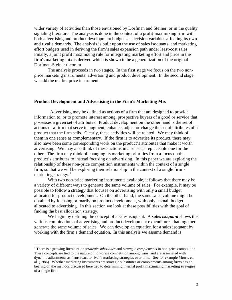
Figure 4 shows the impact of labor-based spin-off production effects tied to product development. Here, since these affect variable production costs, both the ATC and MC curves shift upward as a result of the presence of these impacts on the firm's production process. Note that in this case the vertical shift in both curves is everywhere the same. Also, since marginal cost is involved in this case, increased product development will impact on the firm's production level in two ways. There will be an increase in marginal revenue and there will be an associated increase in marginal costs. As a result, any associated increases in sales and production would be expected to be dampened, relative to cases that do not involve spin-off production effects on labor costs.

10

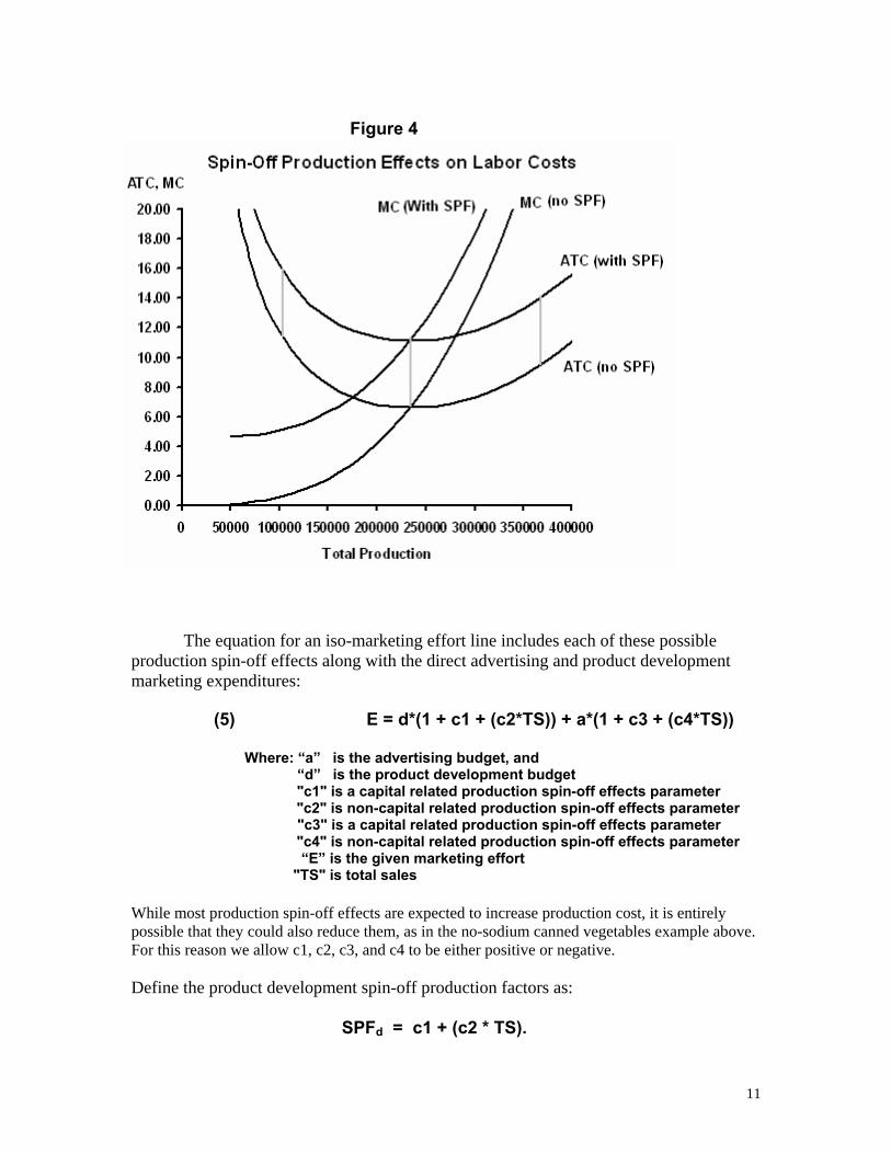
Figure 4

The equation for an iso-marketing effort line includes each of these possible production spin-off effects along with the direct advertising and product development marketing expenditures: (5) E = d*(1 + c1 + (c2*TS)) + a*(1 + c3 + (c4*TS))

Where: “a” is the advertising budget, and “d” is the product development budget "c1" is a capital related production spin-off effects parameter "c2" is non-capital related production spin-off effects parameter "c3" is a capital related production spin-off effects parameter "c4" is non-capital related production spin-off effects parameter “E” is the given marketing effort "TS" is total sales While most production spin-off effects are expected to increase production cost, it is entirely possible that they could also reduce them, as in the no-sodium canned vegetables example above. For this reason we allow c1, c2, c3, and c4 to be either positive or negative. Define the product development spin-off production factors as: SPFd = c1 + (c2 * TS).

11

Similarly, define the advertising spin-off production factors as: SPFa = c3 + (c4 * TS). Properties of Iso-Marketing Effort Lines

• Iso-marketing effort lines are straight lines • Iso-marketing effort lines have a negative slope = – (1+SPFd) / (1+SPFa) • When more than one iso-marketing effort line is plotted on a sales isoquant map,

iso-marketing effort lines for greater marketing efforts lie to the northeast of iso- marketing effort lines for smaller marketing efforts.

• When spin-off production effects increase, the Iso-marketing effort line will rotate to the left around the fixed vertical intercept of a.

Solving equation (5) for a:

This equation for plotting the iso-marketing effort line is of the form y = m*x +b. This is the general form of an equation for a straight line, so we can conclude that iso-marketing effort lines are always linear6. The slope of equation (6) is – (1+SPFd) / (1+SPFa). The vertical intercept of equation (6) is E/(1+SPFa). So a greater marketing effort will entail vertical intercepts located higher on the vertical axis of the sales isoquant map. A greater marketing effort therefore will cause an iso-marketing effort line to “shift” upward and to the right while remaining parallel to an iso-marketing effort line for a smaller marketing effort.

An efficient marketing strategy is the particular combination of advertising and product development expenditures that achieve a given sales goal with the minimum possible marketing effort.

Figure 5 shows how the careful allocation of marketing effort funds between

advertising and product development can impact on the firm’s costs. In the example of Figure 5, product development does not include any production spin-off effects, so in this case, c1 = c2 = c3 = c4 = 0, the slope of each iso-marketing effort line is -1. Four iso-marketing effort lines are plotted on Figure 5 along with a sales isoquant. Each of the selected marketing strategies, points a-g on Figure 5 yield the same sales volume, 122,222 units. 6 Total sales, TS, of course depends on the firm’s advertising and product development expenditures, but in the context of searching for least-cost marketing strategy, total sales is fixed along the target sales isoquant. For this purpose, then, TS is taken as fixed in equation (6).

12

Choosing marketing strategy “a” on Figure 5 requires a total marketing effort of $300,000. Choosing marketing strategy “d” allows the firm to achieve the same sales volume as at point “a” while cutting the total marketing effort to only $180,000. Whenever possible the firm will want to direct the marketing division to adopt marketing strategies like “d” in Figure 5 while avoiding strategies like “a”. Notice that of all the marketing strategies a-g shown on Figure 5, only strategy “d” is a point of tangency between the target sales isoquant and an iso-marketing effort line that provides enough funding to generate the target sales level. For all other possible marketing strategies, the relevant iso-marketing effort line intersects and is not tangent to the target sales isoquant. Since point “d’ is a point of tangency between the target sales isoquant and an iso-marketing effort line, no other strategy will be possible at a lower cost. Strategy “d” is defined as a least-effort marketing strategy yielding 122,222 in total sales. A least-effort marketing strategy should always be preferred to any other possible marketing strategy that yields the same target sales volume.

Since a least-effort marketing strategy is a point of tangency between the target sales isoquant and the minimum possible iso-marketing effort line, the slope of the sales isoquant will be equal to the slope of the cost-minimizing iso-marketing effort line at the point of tangency. Figure 5

13

The slope of the sales isoquant is – MRMS = - MSd / MSa. The slope of the iso-marketing effort line is – (1 SPFd)/(1+SPFa). For least-effort marketing strategies, we therefore know that - MRMS = - MSd / MSa = – (1 + SPFd)/(1+SPFa) and (7) MRMS = MSd / MSa = (1 + SPFd)/(1+SPFa) The Economic Significance of the Least-Effort Marketing Strategy Solution

We have shown that the left side of equation (7a) is the negative of the slope of the sales isoquant and that this will always be equal to the ratio of marginal sales from product development divided by the marginal sales of advertising. The right hand side of equation (7a) is the negative of the slope of the non-price competition Iso-Marketing effort line. (8) MSd / MSa = (1 + SPFd) / (1+SPFa) Equation (8) states that for all least effort marketing strategies, the relative productivity of the marketing instruments will equal their relative cost. Equation 8 may be rearranged to show that with all least effort marketing strategies, sales productivity per dollar spent must be equal across all instruments. (9) MSd / (1 + SPFd) = MSa / (1+SPFa) We will use this relationship to derive an equation for plotting the sales expansion path for the firm in the following section. Equations (8) and (9) determine the relative intensity of advertising and product development in the firm's non-price marketing mix. In this sense we are viewing advertising and product development as substitutes in the firm's non-price marketing mix. Least-effort marketing strategies that lie along the northwest portion of a sales isoquant reflect an advertising intensive non-price marketing mix. Conversely, least-effort marketing strategies that lie along the southeast portion of a sales isoquant reflect a product development intensive non-price marketing mix. Least effort marketing strategies lean toward more instrument neutral non-price marketing mixes.

14

The Firm’s Sales Expansion Path We have seen that there are an infinite number of possible marketing effort strategies to generate any given sales level. Out of all these possibilities, only one strategy qualifies as the least-effort marketing strategy. Before turning to profit maximizing marketing analysis, we will explore the likely character of the firm’s “sales expansion path”, the way the firm should expand or contract its marketing effort, ensuring the use of least-effort marketing strategies along the way.

The firm’s Sales Expansion Path isolates least-effort marketing strategies for each possible volume of sales. We can reveal the firm’s sales expansion path by working with equation (8).

MSa = ΔTS / Δa, and MSd = ΔTS / Δd. As Δ 0, these are the partial derivatives of TS, equation 4, with respect to a and d, respectively:

δTS / δd = Ed * d(Ed-1) * a(Ea) * DS|a,d δTS / δa = Ea * a(Ea-1) * d(Ed) * DS|a,d

and

Substituting (13) into (8):

(Ed * a) / (Ea * d) = (1+SPFd) / (1+SPFa) Solving for a: (14 ) a = (Ea / Ed) * (1+SPFd) / (1+SPFa) * d

15

This is the equation that traces out the firm’s sales expansion path. The nature of the firm's sales expansion path depends on the existence and type of production spin-off effects tied to product development activities. When there are no production spin-off effects, the sales expansion path is of the form y = m*x + b. The vertical intercept is 0, and the slope is Ea/ Ed. In this case, the firm’s sales expansion path is linear. The slope will be completely determined by the relative productivity of the marketing instruments. Moves along the firm's sales expansion path will always involve positively correlated adjustments in advertising and product development. In this sense, we may view advertising and product development as complements. This will be the case independent of any interest the firm may have in using advertising as a "signal" of product quality. Returns to Scale in Marketing Effort The firm's sales expansion path may be used to derive a yield-effort function that shows the relationship between optimized marketing effort and sales yield along the firm's sales expansion path. Begin by solving (1) for d and substitute into (14a) to eliminate d:

Solve for a:

a similar process yields:

Substitute (14a) and (14b) into (5) to get optimized marketing effort, with advertising and product development chosen so that the firm is always on its sales expansion path7. After some algebra:

7 Equation (14c) may also be obtained using methods reviewed in Pyndyck and Rubinfeld (2005) using the method of Lagrange multipliers.

16

In principle, the optimized effort function, (14c) may be solved for sales, TS,

providing an analytical expression for the sales yield-marketing effort relationship. Unfortunately this is not possible, due to the form of SPFa and SPFd used in this analysis. When c2 and c4 are non-zero, however, results may be obtained with simple numerical methods reviewed in Appendix 2. With c2 = c4 = 0, (14c) can be solved analytically for TS. The resulting expression is the sales yield-marketing effort relationship that holds along the firm's sales expansion path, when C2 = C4 = 0.

Under these conditions, we see that returns to scale in sales yield depends on

Ed + Ea, as expected. when Ed + Ea > 0 (14b) implies that there will be increasing returns to scale along the firm's sales expansion path. A doubling in marketing effort will lead to a greater than doubling in sales. When Ed + Ea = 1, equation (14d) implies the firm will experience constant returns to scale along the firm's sales expansion path. A doubling of marketing effort will lead to a doubling of sales. Finally if Ed + Ea < 1 (14d) implies the firm will experience decreasing returns to scale along the firm's sales expansion path. Here a doubling of marketing effort would lead to a less than doubling of sales. When c2 and/or c4 are nonzero, information on Ea and Ed is not sufficient to establish the nature of returns to scale in marketing effort. This will be illustrated in the examples of Figure 6 a-f below.

Marginal sales of marketing effort is defined as the extra sales made possible due

to expanding the firm's marketing effort by one extra dollar. This is found by taking the derivative of the firm's sales yield-marketing effort relation with respect to total sales. The result for the case where c2 = c4 = 0 using equation (14d) is shown here. When c2 and c4 are non-zero, results may be obtained with simple numerical methods reviewed in Appendix 2.

Under these conditions, with constant returns to scale when Ed+Ea = 1, MSe has a

slope of zero. When the firm has increasing returns to scale with Ea+Ed >1. MSe has a slope greater than zero. With decreasing returns, with Ea +Ed < 1, MSe has a slope that is less than zero. When c2 and/or c4 are nonzero, information on Ea and Ed is not sufficient to establish the nature of the slope of the marginal sales of effort function. This will be illustrated in the examples of Figure 6 a-f below.

17

Examples of Instrument Productivity and Spin-off Production Effects on Iso-Effort Lines, the Sales Expansion Path, and Marketing Effort Sales Yield

Figure 6a shows instrument-neutral marketing conditions. In this case there are

no production spin-off effects and sales productivity is equal across marketing instruments with Ea = Ed = 0.4. Here, the slope of the iso-marketing effort line is -1/1, and marginal sales curves are identical for both advertising and product development. Least-effort marketing strategies would always entail equal expenditures on advertising and product development and the sales expansion path has a slope of +1. Since c2 = c4 = 0, Ea + Ed determines returns to scale in marketing effort, which in this case is decreasing returns. This is reflected in the marketing effort sales yield curve and in the marginal sales of marketing effort curve.

Figure 6b shows advertising-intensive marketing conditions. Again there are no production spin-off effects. Here Ea = 0.4, and Ed = 0.1. In this case, advertising expenditures are more productive than product development expenditures in increasing sales. The sales expansion path is linear with a slope greater than one. While the iso-effort line remains unchanged compared with Figure 6a, the sales isoquant rotates counter clockwise giving rise to the change in slope of the sales expansion path. Since c2 =c4 =0, Ea + Ed determines returns to scale in marketing effort, which in this case exhibits more severe decreasing returns than in 6a as expected. This is also reflected in the relatively depressed marginal sales of marketing effort curve as compared with 6a. Similar results would be shown with the productivity differential reversed.

With production spin-off effects that involve capital costs the sales expansion path will also be linear, but the slope will be determined in part by the extent and size of the production spin-off effects on capital inputs. Figure 6c shows a case in which sales productivity is equal across instruments, but the presence of capital-based production spin-off effects tied to product development expenditures results in a linear sales expansion path with slope greater than 1 resulting in advertising intensive marketing conditions. The presence of spin-off production effects tied to capital inputs causes the iso-effort line with these included to rotate. The spin-off production costs impose an added opportunity cost on the use of product development in the marketing mix. Now a dollar spent on product development will be less productive, because a portion of that dollar will be used to address production spin-off effects, and therefore will not be available for direct generation of sales. Since the production spin-off effects in this example are tied to product development only, the advertising endpoint of the iso-effort line is not affected. As a result of spin-off production effects, the reader may be able to verify that the cost-minimizing solution along the 800000 sales isoquant would involve a move to the north west. The opportunity cost tied to production spin-off effects is reflected in the marketing effort sales yield function, and also in the marginal sales of marketing effort function.

18

With production spin-off effects tied to Product development expenditures involving non-capital inputs, the sales expansion path will be non-linear8. With increased production, the cost of engaging in product development increases, and the sales expansion path will tend to fade away from product development toward relatively more advertising intensive marketing strategy. This is illustrated in Figure 6d. Here sales productivity across instruments is once again equal, but the presence of labor based production spin-off effects tied to the product development budget results in a non-linear sales expansion path that adds to advertising intensiveness in marketing as sales increase. As a result of spin-off production effects, the reader may be able to verify that the cost-minimizing solution along the 800000 sales isoquant would again involve a move to the north west. We also observe a significant difference in the impact of spin-off production effects tied to the labor input in both marketing effort sales yield and in the marginal sales of marketing effort functions. In each of these the opportunity cost increases relatively more with increases in marketing effort with spin-off effects tied to labor inputs as compared to spin-off effects tied to capital inputs. The difference is most dramatic in the marginal sales of marketing effort function. Here the shift tied to spin-off effects rooted in capital inputs is relatively unchanged with increased marketing effort in Figure 6c, whereas it dramatically increases with spin-off effects tied to labor inputs in Figure 6d. Finally, Figure 6e like 6d includes labor based production spin-off effects on product development expenditures, but these are negative and reduce production costs. With sales productivity equal across instruments, this leads to a non-linear sales expansion path that adds to product development intensiveness as sales increase. In this case the spin-off effect on production is a reduction in production cost. Because of this, the iso-effort line in figure 6e rotates in the opposite direction compared to Figure 6d. This would lead to a product development-intensive marketing mix. Note that as was true with Figure 6d, these effects intensify quite dramatically as marketing effort is increased. Spin-off production effects are sufficiently strong in this example to change economies of scale in marketing effort from decreasing to increasing returns. This is true despite the fact that Ea +Ed continue to equal .8 as in Figures 6 b-d.

Obviously there are a rich variety of possible marketing conditions in this model. These entail various combinations of marketing productivity conditions and production spin-off effects. Production spin-off effects shown in the above examples have been tied to product development expenditures only. Similar effects are possible involving production spin-off effects tied to advertising, and to combinations involving both non-price marketing instruments.

8 Note that when we address the character of the sales expansion path, then TS will be variable giving rise to the possibility of a non-linear shape. This is in contrast to the least-effort marketing strategy analysis for which TS is taken as fixed.

19

20

Figure 6a: Instrument Nuetral Marketing Conditions

Epmine -4Epthem 2.5Eamine 0.4Eathem -0.36EDmine 0.4EDthem -0.36EY 1.17EPs 0.95EPc -1.1EE 1EC 1

c1 0c2 0

Advertising Sales Yield

0

100000

200000

300000

400000

500000

600000

700000

800000

900000

0 50000 100000 150000 200000Advertising Expenditures

Total Sales

Marginal Sales of Advertising

0.000.501.001.502.002.503.003.504.004.505.00

0 50000 100000 150000 200000

Advertising Expenditures

MSa

Product Development Sales Yield

0

100000

200000

300000

400000

500000

600000

700000

800000

900000

0 50000 100000 150000 200000

Product Development Expenditures

Total Sales

Marginal Sales of Product Development

0.00

0.50

1.00

1.50

2.00

2.50

3.00

3.50

4.00

4.50

5.00

0 20000 40000 60000 80000 100000 120000 140000 160000 180000 200000


MSpd

Sales Isoquant and Expansion Path

0

100000

200000

300000

400000

500000

600000

0 100000 200000 300000 400000 500000 600000Product Development

Advertising

TS = 800000Sales Ex. PathIso-EffortIso-Effort (no SPF)

Marketing Effort Sales Yield

0

200000

400000

600000

800000

1000000

1200000

1400000

1600000

0 100000 200000 300000 400000 500000 600000 700000 800000Marketing Effort

Sale

s Yi

eld

Marginal Sales of Marketing Effort

0

0.5

1

1.5

2

2.5

3


MSe

21

Figure 6b: Advertising Intensive Marketing Conditions


c1 0c2 0


0

100000

200000

300000

400000

500000

600000

700000

800000

900000


Total Sales


0.000.501.001.502.002.503.003.504.004.505.00

0 50000 100000 150000 200000


MSa


0

100000

200000

300000

400000

500000

600000

700000

800000

900000

0 50000 100000 150000 200000Product Development Expenditures

Total Sales


0.000.501.001.502.002.503.003.504.004.505.00

0 50000 100000 150000 200000


MSpd


0

100000

200000

300000

400000

500000

600000


Advertising



0

200000

400000

600000

800000

1000000

1200000

1400000

1600000


Sale

s Yi

eld


0

0.5

1

1.5

2

2.5

3


MSe

22

Figure 6c: Advertising Intensive Marketing Conditions


c1 1c2 0


0

100000

200000

300000

400000

500000

600000

700000

800000

900000


Total Sales


0.000.501.001.502.002.503.003.504.004.505.00

0 50000 100000 150000 200000


MSa


0

100000

200000

300000

400000

500000

600000

700000

800000

900000


Total Sales


0.000.501.001.502.002.503.003.504.004.505.00

0 50000 100000 150000 200000


MSpd


0

100000

200000

300000

400000

500000

600000


Advertising



0

200000

400000

600000

800000

1000000

1200000

1400000

1600000

0 100000

200000

300000

400000

500000

600000

700000

800000

Marketing Effort

Sale

s Yi

eld

Yield-Effort with SPFYield-Effort no SPF


0

0.5

1

1.5

2

2.5

3

0 200000 400000 600000 800000Marketing Effort

MSe

MSe with SPFMSe with SPF

23

Figure 6d: Advertising Intensive Marketing Conditions


c1 0c2 0.000002


0

100000

200000

300000

400000

500000

600000

700000

800000

900000


Total Sales


0.000.501.001.502.002.503.003.504.004.505.00

0 50000 100000 150000 200000


MSa


0

100000

200000

300000

400000

500000

600000

700000

800000

900000


Total Sales


0.000.501.001.502.002.503.003.504.004.505.00

0 50000 100000 150000 200000


MSpd


0

100000

200000

300000

400000

500000

600000


Advertising



0

200000

400000

600000

800000

1000000

1200000

1400000

1600000

0 100000

200000

300000

400000

500000

600000

700000

800000

Marketing Effort

Sale

s Yi

eld



0

0.5

1

1.5

2

2.5

3


MSe


24

Figure 6e: Product Development Intensive Marketing Conditions


c1 0c2 -4E-07


0

100000

200000

300000

400000

500000

600000

700000

800000

900000


Total Sales


0.000.501.001.502.002.503.003.504.004.505.00

0 50000 100000 150000 200000


MSa


0

100000

200000

300000

400000

500000

600000

700000

800000

900000


Total Sales


0.000.501.001.502.002.503.003.504.004.505.00

0 50000 100000 150000 200000


MSpd


0

100000

200000

300000

400000

500000

600000


Advertising



0

200000

400000

600000

800000

1000000

1200000

1400000

1600000

0 100000

200000

300000

400000

500000

600000

700000

800000

Marketing Effort

Sale

s Yi

eld



0

0.5

1

1.5

2

2.5

3


MSe


25

Joint Profit Maximization Over Price and Marketing Effort In this section we derive a rule for joint profit maximizing over both setting price and for allocating funds to the firm’s marketing effort. We assume the firm must choose price, P, and its marketing effort, E to maximize profits. In addition, we assume that advertising and product development budgets are chosen so as to keep the firm on its sales expansion path with the minimum possible marketing effort. Specific parameter values used in this analysis are listed in Appendix 1 and Appendix 2. Keeping in mind that since marketing effort can increase the firm’s demand, but also adds to costs, the firm’s profit function is: (17) π = P * TS*( P,E ) - TC( TS* ) – E where E is the budget allocated for marketing effort expenditures, P is the firm’s price, and TS* is given by (14d) when c2 = c4 = 0. First order conditions are: (21) P * MS*

P + TS - MC * MS*p = 0, and

(22) P * MS*

E - MC * MS*E - 1 = 0,

where: MS*

P = δTS*/ δP, and MS*

E = δTS*/ δE (14e) when c2 = c4 = 0. Solve (21) and (22) for P, and set the resulting expressions equal to eliminate P. Then cancel MC from both sides:

Invert both sides:

Multiply by P:

26

The left-hand side of (24) is the absolute value of the firm’s price elasticity of demand:

Equation (25) is the Dorfman-Steiner Theorem generalized to accommodate product development and advertising as defined for this study. It states that profits are maximized when the firm engages marketing effort (with advertising and product development restricted to the firm's sales expansion path) to the point where the value of the marginal product of marketing effort per dollar spent equals the firm’s price elasticity of demand.

The intuition behind equation (25) is not at all obvious. Actually equation (24) provides most straightforward interpretation. The left side of equation (24) is the value of marginal sales per dollar spent in increasing sales by reducing the firm’s price. Reducing the price by one dollar will cost the firm TS dollars altogether, since each of the products sold will have required a price reduction. This actually compares quite easily with the right side of equation (24). The right side is the value of the marginal sales per dollar spent on marketing effort.

Where:

VMSP is the value of marginal sales per dollar spent in price reduction, and VMSE is the value of marginal sales per dollar spent on marketing effort.

Equation (26) states that a profit maximizing marketing strategy requires that the value of the marginal sales per dollar spent be equal across marketing instruments. Figure 7 illustrates the relationship summarized by equation (26). Since we are working with a constant price elasticity of demand model in this analysis, we know that the left side of equation (26) is constant and equal to the firm’s price elasticity of demand. This is shown in Figure 7 as the horizontal line. The downward sloping line in Figure 7 is VMSE per dollar spent.

27

Figure 7

If the firm's price elasticity of demand is - 4 and elastic, we would expect that the firm would reduce its price in order to increase total sales revenue9. Since the value of marginal sales per dollar spent when dropping price is 4, it would seem that the firm should go ahead and reduce its price, since each dollar lost tied to the reduction in price would be rewarded with four dollars in added sales revenue. With elastic demand, the firm adds to sales revenue by reducing its price. Equation (26), however, implies that this may not necessarily always be what the firm should do. If the value of marginal sales per dollar spent on marketing effort is greater than 4, (with E < E*) then the firm should increase marketing effort and market price instead of decreasing price10. This would be the proper adjustment even when the firm's price elasticity of demand is -4!

Whenever the value of marginal sales tied to reducing the price per dollar spent is less than the value of marginal sales tied to marketing effort per dollar spent, then the firm should increase marketing effort and its price, even if demand is price elastic. This will tend to decrease VMSE per dollar spent so that it comes in line with the VMSp per dollar spent. On the other hand, if the value of marginal sales tied to reducing the price per dollar spent (the firm's price elasticity of demand) is greater than the value of marginal sales tied to marketing effort per dollar spent, then the firm should reduce price and reduce its marketing effort. This will tend to increase VMSE per dollar spent so that it

9 The reader should note that we are comparing prices vs. marketing effort in generating sales. Equations (21) and (22) correctly shows that the full marginal cost of engaging in each of these instruments would also be considered, and this involves the production costs tied to increasing sales. Since this would be shared equally across marketing instruments, these costs have cancelled out in the process of deriving equations (24), (25), and (27). 10 This is because marginal revenue is increased with an increase in marketing effort.

28

comes in line with the VMSp per dollar spent. These results are conditioned on the assumptions about expected marketing effort and price of rival firms. In addition, these results are based on the assumption that $11.04 is the profit maximizing price decision of the firm under study. When the firm adjusts its marketing effort based on a given price, this adjustment must be in turn be added to the profit maximization analysis for the firm’s output and price. When equation (27) calls for an increase in marketing effort, there will be an associated increase in the profit maximizing price, and that in turn will have to be considered in a revised profit maximizing marketing effort decision. There will be an iterative approach to the profit maximizing decisions. This requires a simultaneous solution for optimal price and marketing effort decisions. Figure 8 shows the resulting impact on the optimal value of marginal sales tied to an added dollar spent on marketing effort. If the firm finds that with E1 marketing effort is less than the profit maximizing marketing effort based on using P1 for its price, it will want to increase marketing effort, by moving for example from point A to point B, increasing its marketing effort from E1 to E2. This new marketing effort will call for a higher price for profit maximization. Other things equal, however, and increase in the firm's price will reduce sales. This implies point B will not in fact be optimal. The increase in the firm's price will reduce the VMSE per dollar spent on marketing effort, and the proper adjustment will be from point A to point C on Figure 8 in increasing marketing effort from E1 to E2

11. Marketing effort will in fact be less responsive. Since VMSE/(1 + PD/E * SPF) as graphed in figure 7, above, is based on a fixed price, the actual optimal curve based on a variable price will be more steeply sloped.

11 Since VMSE = P * MSE , this result is not transparent since an increase in price also exerts a positive impact on VMSE . Note that equation (1) shows PP

Ep as part of the shifter term. This term is preserved with MS . Multiplying by P, we get P * PE

Ep = P(1 +Ep). This is the total impact that P has on VMS . With Elastic demand, (1 + E ) must be negative, so any increase in P will have an unambiguously negative impact on VMS . With E <= 1, Profit maximization is undefined.

E

p

E p

29

Figure 8

Based on figures 7 and 8, it is quite easy to see that an increase in price elasticity of demand should lead to a reduction in marketing effort and greater reliance on price reductions for increasing sales. This would occur for two reasons. First, the value of marginal sales per dollar spent on price reduction ,VMSP per dollar spent, would shift upward, leading to a reduction in optimal marketing effort.

An increase in price elasticity of demand will also impact on VMSE per dollar spent on marketing effort. If an increase in price reduces the value of marginal sales per dollar spent on marketing effort, an increase in the price elasticity of demand must increase this effect by increasing buyer sensitivity to price changes. This means that an increase in the firm's price elasticity of demand will decrease VMSE per dollar spent on marketing effort. This will also lead to reduced marketing effort other things equal.

An increase in the firm's price elasticity of demand will shift VMSE per dollar spent on marketing effort downward while shifting the VMSP per dollar spent on price reductions upward. These combined impacts will lead to reduced marketing effort by a profit maximizing firm with an increase in the firm's price elasticity of demand. This is the expected result. An extreme case would be observed when the firm's demand is nearly perfectly elastic, and marketing effort would not be observed among profit maximizing firms.

An increase in the firm's advertising elasticity or product development elasticity will increase the firm's VMSE per dollar spent. These changes will always lead to an increase in marketing effort and an increase in the firm's price.

30

Conclusions This paper develops a positive analysis of marketing mix theory in the context of

coordinating advertising, product development and price instruments by firms. The analysis was built upon the use of “sales isoquants”, and “marketing effort” budgets used in generating firm level “least-cost sales”. This in turn was used in deriving the firm’s “sales expansion path”. Finally, a profit maximizing rule for optimal marketing effort expenditures was derived which was shown to be a generalization of the Dorfman-Steiner theorem.

This approach to the joint optimization problem over three marketing decision variables is useful for two primary reasons. First, the method explores the complements / substitutes dual nature that advertising and product development play in the optimal marketing mix of the firm irrespective of any "signaling" intent. Second, the approach allows the analyst to reduce the number of marketing decision variables from three (price, advertising, and product development) to two (price, and marketing effort). This greatly reduces the complexity of identifying profit maximization solutions.

The profit-maximizing rule for the price / marketing effort mix derived in this paper is shown to be a generalization of the Dorfman-Steiner Theorem. A re-thinking of the information inherent in the price elasticity of demand leads to the fundamental result of this paper. Marketing effort should always be expanded along the firm’s sales expansion path up to the point where the value of the marginal sales per dollar spent in price reduction equals the value of the marginal sales per dollar spent on marketing effort. Restricting marketing effort to advertising and product development expenditures that lie on the firm's expansion path allows for an unambiguous connection between dollars allocated to marketing effort and the corresponding upper limit on sales. This result has a straightforward intuitive appeal and lends itself to straightforward comparative static analysis of the firm's profit maximizing marketing mix.

31

Appendix 1: Parameter Values Used in the Firm’s Demand Function Graphs and tables presented in this paper are based on the following assumptions as defined for equation (1) in the text: Table A-1 Parameters Figure 1 Figure 6a Figure 6b Figure 6c Figure 6d Figure 6e Figure 7 Table A-1

C 30 30 30 30 30 30 30 30p 9.6 10 10 10 10 10 11.04 11.0

ap(c) 8 10 10 10 10 10 11.04 11.0aa(c) 150000 200000 200000 200000 200000 200000 594737.63 594737.63ad(c) 150000 200000 200000 200000 200000 200000 764662.67 764662.67

Y 30000 30000 30000 30000 10 30000 30000 30000Ps 5.5 5.5 5.5 5.5 10 5.5 5.5 5.5Pc 200 200 200 200 200 200 200 200c1 0 0 0 1 0 0 0 0c2 0 0 0 0 0.000003 -0.0000004 0 0c3 0 0 0 0 0 0 0 0c4 0 0 0 0 0 0 0 0Ep -0.4 -0.4 -0.4 -0.4 -0.4 -0.4 -0.4 -0.4

Eap(c) 2.5 2.5 2.5 2.5 2.5 2.5 2.5 2.5Ea 0.35 0.4 0.4 0.4 0.4 0.4 0.35 0.35

Eaa(c) -0.31 -0.36 -0.36 -0.36 -0.36 -0.36 -0.31 -0.31Ed 0.45 0.4 0.1 0.4 0.4 0.4 0.45 0.45

Ead(c) 0.41 -0.36 -0.06 -0.36 -0.36 -0.36 0.41 0.41EY 1.17 1.17 1.17 1.17 1.17 1.17 1.17 1.17EPc -1.1 -1.1 -1.1 -1.1 -1.1 -1.1 -1.1 -1.1Eps 0.95 0.95 0.95 0.95 0.95 0.95 0.95 0.95

44

32

Appendix 2

The Profit Maximizing Marketing Effort Analysis table, Table 1, makes use of equation (24) in determining the profit maximizing marketing effort. Parameter values used in calculating the results presented in Table A-2 are listed in Appendix 1. Table A-2:

The data of Table 2 are calculated with the following method. First Total Sales listed in column 2 is incremented by 116029 row by row beginning with 75000 in row one. Given this series for total sales in column 2, A* and D* are calculated for each row using equations (14a) and (14b). Marketing effort is then calculated in column 1 using data on TS, A*, and PD* using equation (5). Marginal sales (MS*

E) per added marketing effort dollar spent is listed in column 5. This is calculated as follows: MS*

E = ΔTS* / ΔE Marginal sales on row 2 is calculated by taking differences in these variables between rows 3 and 1:

33

Where: numbers in parenthesis are table row numbers This differencing method of calculating Marginal sales per dollar spent on marketing effort (MS*

E) is extremely accurate, and may be used regardless of the values of c2 and c4. The value of marginal sales per dollar spent on marketing effort, VMSe / 1 is

calculated by multiplying product price times marginal sales per marketing effort dollar spent. This is listed in column 7: VMSE / 1 = (MS*

E * P) / 1 Finally, the value of marginal sales per dollar spent on price reduction, VMSp / TS, is calculated by multiplying product price times marginal sales per dollar spent on price reduction. This is listed in column 8: VMSP / TS = (MS*

P * P) / TS

34

References:

Dorfman and Steiner. 1954. “Optimal Advertising and Optimal Quality”. American Economic Review, December 1954, p. 834.

Kihlstrom, Richard E. and Michael H. Riordan 1978. "Advertising as a Signal." Journal of Political Economy 92:427-450.

Kwoka, John E. 1993. "the Sales and Competitive Effects of Styling and Advertising Practices in the U. S. Auto Industry." The Review of Economics and Statistics 75:649-656.

Landes, Elizabeth M. and Andrew M. Rosenfield 1994. "The Durability of Advertising Revisited." The Journal of Indusial Economics 42:263-276.

Harvey Leibenstein, "Allocative Efficiency and X-Efficiency," The American Economic Review, 56 (1966), pp. 392-415.

Morris, D.J., P.J.N. Sinclair, M.D. E. Slater, and J.S. Vickers 1986. "Strategic Behavior and Industrial Competition: An Introduction." Oxford Economic Papers, New Series Vol. 38, Supplement: Strategic Behavior and Industrial Competition. pp.1-8

Nelson, Phillip. 1970. "Information and Consumer Behavior." Journal of Political Economy 78:311-29.

_____. 1974. "Advertising as Information." Journal of Political Economy 81:729-54.

_____. 1978. "Advertising as Information Once More." In Issues in Advertising: The Economics of Persuasion, edited by D.C. Tuerck. Washington: American Enterprise Inst.

Nichols, Mark W. 1998. "Advertising and Quality in the U.S. Market for Automobiles." Southern Economic Journal, 64:922-939.

Pindyck, Robert S. and Daniel Rubinfeld. 2005. Microeconomics 6 ed., Pearson Education Inc., Upper Saddle River, N.J.

Schmalensee, Richard. 1978. "A Model of Advertising and Product Quality." Journal of Political Economy 86:485-503.

Von der Fehr, Nils-Henrik M., and Kristen Stewvik. 1998. "Persuasive Advertising and Product Differentiation." Southern Economic Journal 65:113-126.

35

Documents

Marketing Mix Theory: Integrating Price and Non … Mix Theory: Integrating Price and Non-Price Marketing Strategies William C. Kolberg Department of Economics Ithaca College Introduction