Market Structure and Competition in Airline Markets

⇤

Federico Ciliberto†

University of VirginiaCharles Murry‡

Penn State UniversityElie Tamer§

Harvard University

May 9, 2016

Abstract

We provide an econometric framework for estimating a game of simultaneous entry and

pricing decisions in oligopolistic markets while allowing for correlations between unobserved

fixed costs, marginal costs, and demand shocks. Firms’ decisions to enter a market are based

on whether they will realize positive profits from entry. We use our framework to quantitatively

account for this selection problem in the pricing stage. We estimate this model using cross-

sectional data from the US airline industry. We find that not accounting for endogenous entry

leads to overestimation of demand elasticities. This, in turn, leads to biased markups, which

has implications for the policy evaluation of market power. Our methodology allows us to study

how firms optimally decide entry/exit decision in response to a change in policy. We simulate a

merger between American and US Airways and we find: i) the price e↵ects of a merger can be

strong in concentrated markets, but post-merger entry mitigates these e↵ects; ii) the merged

firm has a strong incentive to enter new markets; iii) the merged firm faces a stronger threat

of entry from rival legacy carriers, as opposed to low cost carriers.

⇤We thank Timothy Bresnahan, Ambarish Chandra, John Panzar, Wei Tan, Randal Watson, and JonWilliams for insightful suggestions. We also thank participants at the Southern Economic Meetings inWashington (2005 and 2008), the 4th Annual CAPCP Conference at Penn State University, 2009, theJournal of Applied Econometrics Conference at Yale in 2011, and the DC Industrial Organization Conferencein 2014, where early drafts of this paper were presented. Seminars participants at other institutions provideduseful comments. Finally, we want to especially thank Ed Hall and the University of Virginia Alliance forComputational Science and Engineering, who have given us essential advice and guidance in solving manycomputational issues. We also acknowledge generous support of computational resources from XSEDEthrough the Campus Champions program (NSF-Xsede Grant SES150002).

†Department of Economics, University of Virginia, ciliberto@virginia.edu. Federico Ciliberto thanksthe CSIO at Northwestern University for sponsoring his visit at Northwestern University. Research supportfrom the Bankard Fund for Political Economy at the University of Virginia and from the QuantitativeCollaborative of the College of Arts and Science at the University of Virginia is gratefully acknowledged.

‡Department of Economics, Penn State, cmurry@psu.edu.§Department of Economics, Harvard University, elietamer@fas.harvard.edu

1

1 Introduction

We estimate a simultaneous, static, complete information game where economic agents make

both discrete and continuous choices. The methodology is used to study airline firms that

strategically decide whether to enter into a market and the prices they charge if they enter.

Our aim is to provide a framework for combining both entry and pricing into one empirical

model that allows us: i) to account for selection of firms into serving a market (or account

for endogeneity of product characteristics) and more importantly ii) to allow for market

structure (who exits and who enters) to adjust as a response to counterfactuals (such as

mergers).

Generally, firms self-select into markets that better match their observable and unobserv-

able characteristics. For example, high quality products command higher prices, and it is

natural to expect high quality firms to self-select themselves into markets where there is a

large fraction of consumers who value high-quality products. Previous work has taken the

market structure of the industry, defined as the identity and number of its participants (be

they firms or, more generally, products or product characteristics), as exogenous, and esti-

mated the parameters of the demand and supply relationships.1 That is, firms, or products,

are assumed to be randomly allocated into markets. This assumption has been necessary to

simplify the empirical analysis, but it is not always realistic.

Non-random allocation of firms across markets can lead to self-selection bias in the estima-

tion of the parameters of the demand and cost functions of the firms. Existing instrumental

variables based methods to account for endogeneity of prices do not resolve this selection

problem in general. Potentially biased estimates of the demand and cost functions can then

lead to the mis-measurement of market power. This is problematic because correctly mea-

suring market power and welfare is of crucial importance for the application of antitrust

policies and for a full understanding of the competitiveness of an industry. For example, if

the bias is such that we infer firms to have more market power than they actually have, the

antitrust authorities may block the merger of two firms that would improve total welfare,

1 See (Bresnahan, 1987; Berry, 1994; Berry, Levinsohn, and Pakes, 1995).

2

possibly by reducing an excessive number of products in the market. Importantly, allowing

for entry (or product variety) to change as a response say to a merger is important as usually

when a firm (or product) exits, it is likely that other firms may now find it profitable to enter

(or new products to be available). Our empirical framework allows for such adjustments.

Our model can also be viewed as a multi-agent version of the classic selection model

(Gronau, 1974; Heckman, 1976, 1979). In the classic selection model, a decision maker

decides whether to enter the market (e.g. work), and is paid a wage conditional on working.

When estimating wage regressions, the selection problem deals with the fact that the sample

is selected from a population of workers who found it “profitable to work.” Here, firms (e.g

airlines) decide whether to enter a market and then, conditional on entry, they choose prices.

As in this single agent selection model, when estimating demand and supply equations, our

econometric model accounts for this selection.

Our model consists of the following equations: i) entry conditions that require that in

equilibrium a firm that serves a market must be making non-negative profits; ii) demand

equations derived from a discrete choice model of consumer behavior; iii) pricing first-order-

conditions, which can be formally derived under the postulated firm conduct. We allow

for all firm decisions to depend on unobservable to the econometrician random variables

(errors) that are firm specific and also market/product specific unobservables that are also

observed by the firms and unobserved by the econometrician. An equilibrium of the model

occurs when firms make entry and pricing decisions such that all three sets of equations are

satisfied.

A set of econometric problems arises when estimating such a model. First, there are

multiple equilibria associated with the entry game. Second, prices and/or product charac-

teristics in the second stage are endogenous as they are associated with the optimal behavior

of firms. These are determined in equilibrium. Finally, the model is nonlinear and so poses

heavy computational burden. We combine the methodology developed by Tamer (2003) and

Ciliberto and Tamer (2009) (henceforth CT) for the estimation of complete information,

static, discrete entry games with the widely used methods for the estimation of demand and

3

supply relationships in di↵erentiated product markets (see Berry, 1994; Berry, Levinsohn,

and Pakes, 1995, henceforth BLP). We simultaneously estimate the parameters of the entry

model (the observed fixed costs and the variances of the unobservable components of the

fixed costs) and the parameters of the demand and supply relationships.

To estimate the model we use cross-sectional data from the US airline industry.2 The

data are from the second quarter of 2012’s Airline Origin and Destination Survey (DB1B).

We consider markets between US Metropolitan Statistical Areas (MSAs), which are served

by American, Delta, United, USAir, Southwest, and low cost carriers (e.g. Jet Blue). We

observe variation in the identity and number of potential entrants across markets.3 Each

firm makes decides whether or not to enter and chooses the (median) price in that market.

The other endogenous variable is the number of passengers transported by each firm. The

identification of the three equations is o↵ the variation of several exogenous explanatory

variables, whose selection is based on a rich and important literature, for example Rosse

(1970), Panzar (1979), Bresnahan (1989), and Schmalensee (1989), Brueckner and Spiller

(1994), Berry (1990), Berry and Jia (2010), Ciliberto and Tamer (2009), and Ciliberto and

Williams (2014). More specifically, we consider market distance and measures of the airline

network, both nonstop and connecting of airlines out of the origin and destination airports.

We begin our empirical analysis by running a standard GMM estimation (see Berry, 1994)

on the demand and pricing first order conditions for multiple specifications, allowing for

di↵ering levels of heterogeneity in the model. Next, we estimate the model with endogenous

entry using our methodology and compare the results with the GMM results. We find that

using our methodology the price coe�cient in the demand function is estimated to be closer

to zero than the case of GMM, and markups are on the order of 60% larger than the GMM

results imply. The parameters in the fixed cost equation are precisely estimated and they are

decreasing in measures of network size at the origin and destination airport. We examine the

fit of our models along three dimensions: i) the predicted market structures; ii) the predicted

2We also illustrate our methodology by conducting a Monte Carlo exercise, see the Online Supplement.3An airline is considered a potential entrant if it is serving at least one market out of both of the endpoint

airports.

4

prices; iii) the predicted market shares.4 Additionally, we estimate significant correlations

between unobserved fixed costs, unobserved marginal costs, and unobserved demand shocks.

Finally, we use our estimated model to simulate the merger of two airlines in our data:

American and US Airways.5 Typical merger analysis involves predicting changes in market

power and prices given a particular market structure using diversion ratios based on pre-

merger market shares, or predictions from static models of product di↵erentiation (see Nevo,

2000). Our methodology allows us to simulate a merger allowing for equilibrium changes

to market structure after a merger, which in turn may a↵ect equilibrium prices charged by

firms. Market structure reactions to a merger are an important concern for policy makers,

such as the DOJ, as they often require entry accommodation by merging firms after the

approval of a merger. For example, in the two most recent large airline merger (United and

American), the DOJ required the merging firms to cede gate access at certain airports to

competitors. Our methodology can help policy makers understand how equilibrium entry

would change after a merger, which would in turn help target tools like the divestiture of

airport gates.

In our merger simulation we analyze a “best case” scenario where we assign the best

characteristics from the two pre-merger firms to the new merged firm (both in demand and

costs).6 First, we predict that the new merged firm would enter the unserved markets with

a probability of at least 20%. This highlights an important reason to consider endogenous

entry responses after a merger, as entry into new markets is a potentially large source of

additional consumer welfare. Second, we find, as we would expect, that there is a general

tension between higher prices from greater concentration and lower prices from increased

e�ciency and increased entry of the merged firm. Concentrated markets where the merged

firm is an incumbent are at greatest risk for price increases, but there are many cases where

4Unlike the canonical model of demand for di↵erentiated products (see Berry (1994) and BLP) ourmethodology does not by construction perfectly predict prices and shares by inverting a product level demand.

5The two firms merged in 2013 after settling with the Department of Justice.6Our reasoning for choosing to look at the “best case” scenario is that a merger should not be allowed if

there are no gains, even under the ”best case” scenario, whether in the form of lower prices or new entry,after the merger.

5

prices decrease after the merger. Third, we find that the merged firm faces the greatest

competition form rival legacy carriers after the merger. This is because major carriers are

more similar in characteristics to the merged firm than low cost carriers, and so are more

likely to enter markets where the merged firm is an incumbent after the merger.

There is important work that has estimated static models of competition while allowing

for market structure to be endogenous. Reiss and Spiller (1989) estimate an oligopoly

model of airline competition but restrict the entry condition to a single entry decision. In

contrast, we allow for multiple firms to choose whether or not to serve a market. Cohen

and Mazzeo (2007) assume that firms are symmetric within types, as they do not include

firm specific observable and unobservable variables. In contrast, we allow for very general

forms of heterogeneity across firms. Berry (1999), Draganska, Mazzeo, and Seim (2009),

Pakes et al. (2015) (PPHI), and Ho (2008) assume that firms self-select themselves into

markets that better match their observable characteristics. In contrast, we focus on the

case where firms self-select themselves into markets that better match their observable and

unobservable characteristics. There are two recent papers that are closely related to ours.

Eizenberg (2014) estimates a model of entry and competition in the personal computer

industry. Estimation relies on a timing assumption (motivated by PPHI) requiring that

firms do not know their own product quality or marginal costs before entry, which limits the

amount of selection captured by the model. Roberts and Sweeting (2014) estimate a model of

entry and competition for the airline industry, but only consider sequential move equilibria.

In addition, Roberts and Sweeting (2014) do not allow for correlation in the unobservables,

which is the key determinant of self-selection that we investigate in this paper.

The paper is organized as follows. Section 2 presents the methodology in detail in the

context of a bivariate generalization of the classic selection model, providing the theoretical

foundations for the empirical analysis. Section 3 introduces the economic model. Section 4

introduces the airline data, providing some preliminary evidence of self-selection of airlines

into markets. Section 5 shows the estimation results and Section 6 presents results and

discussion of the merger exercise. Section 7 concludes.

6

2 A Simple Model with Two Firms

We illustrate the inference problem with a simple model of strategic interaction between two

firms that is an extension of the classic selection model. Two firms simultaneously make an

entry/exit decision and, if active, realize some level of a continuous variable. Each firm has

complete information about the problem facing the other firm. We first consider a stylized

version of this game written in terms of linear link functions. This model is meant to be

illustrative, in that it is deliberately parametrized to be close to the classic single agent

selection model. This allows for a more transparent comparison between the single vs multi

agent model. Section 3 analyzes a full model of entry and pricing.

Consider the following system of equations,

y

1

= 1 [�2

y

2

+ �Z

1

+ ⌫

1

� 0] ,y

2

= 1 [�1

y

1

+ �Z

2

+ ⌫

2

� 0] ,S

1

= X

1

� + ↵

1

V

1

+ ⇠

1

,

S

2

= X

2

� + ↵

2

V

2

+ ⇠

2

(1)

where yj = 1 if firm j decides to enter a market, and yj = 0 otherwise, where j 2

{1, 2}. Let K ⌘ {1, 2} be the set of potential entrants. The endogenous variables are

(y1

, y

2

, S

1

, S

2

, V

1

, V

2

). We observe (S1

, V

1

) if and only if y1

= 1 and (S2

, V

2

) if and only

if y

2

= 1. The variables Z ⌘ (Z1

, Z

2

) and X ⌘ (X1

, X

2

) are exogenous whereby that

(⌫1

, ⌫

2

, ⇠

1

, ⇠

2

) is independent of (Z,X) while the variables (V1

, V

2

) are endogenous (such as

prices or product characteristics).7

As can be seen, the above model is a simple extension of the classic selection model

to cover cases with two decision makers. The key important distinction is the presence of

simultaneity in the ‘participation stage’ where decisions are interconnected.

We will first make a parametric assumption on the joint distribution of the errors. In

principle, it is possible to study the identified features of the model without parametric

assumptions on the unobservables, but that will lead to a model that is hard to estimate

7It is simple to allow � and � to be di↵erent among players, but we maintain this homogeneity forexposition.

7

empirically. Let the unobservables have a joint normal distribution,

(⌫1

, ⌫

2

, ⇠

1

, ⇠

2

) ⇠ N (0,⌃) ,

where ⌃ is the variance-covariance matrix to be estimated. The o↵-diagonal entries of the

variance-covariance matrix are not generally equal to zero. Such correlation between the

unobservables is one source of the selectivity bias that is important.8

One reason why we would expect firms to self-select into markets is because the fixed

costs of entry are related to the demand and the variable costs. One would expect products

of higher quality to be, at the same prices, in higher demand than products of lower quality

and also to be more costly to produce. For example, a luxury car requires a larger up-

front investment in technology and design than an economy car, and a unit of a luxury car

costs more to produce than a unit of an economy car. This would introduce unobserved

correlation in the unobservables of the demand, marginal and fixed costs. The unobservables

might be correlated if a firm can lower its marginal costs by making investments that increase

its fixed costs but are still profitable. In that case, we would observe a correlation between

the unobservables in the marginal and fixed cost functions.

Given that the above model is parametric, the only non standard complications that arise

are ones related to multiplicity and also endogeneity. Generally, and given the simultaneous

game structure, the system (1) has multiple Nash equilibria in the identity of firms entering

into the market. This multiplicity leads to a lack of a well defined “reduced form” which

complicates the inference question. Also, we want to allow for the possibility that the V ’s

are also choice variables (or variables determined in equilibrium). Throughout, we maintain

the assumption that players are playing pure strategy Nash equilibria. Extending this to

mixed strategy does not pose conceptual problems.

The data we observe are (S1

y

1

, V

1

y

1

, y

1

, S

2

y

2

, V

2

y

2

, y

2

,X,Z) and given the normality as-

sumption, we link the distribution of the unobservables conditional on the exogenous vari-

ables to the distribution of the outcomes to obtain the identified features of the model. The8Also, it is clear that using instrumental variables on the outcome equations in (1) above does not

correct for selectivity in general, since, even though we have E[⇠1|X,Z] = 0, that does not imply thatE[⇠1|X,Z, y1 = 1] = 0.

8

data allow us to estimate the distribution of (S1

y

1

, V

1

y

1

, y

1

, S

2

y

2

, V

2

y

2

, y

2

,X,Z) and the key

to inference is to link this distribution to the one predicted by the model. To illustrate this,

consider the observable (y1

= 1, y2

= 0, V1

, S

1

,X,Z). For a given value of the parameters,

the data allow us to identify

P (S1

+ ↵

1

V

1

�X

1

� t

1

; y1

= 1, y2

= 0|X,Z) (2)

for all t1

. The particular form of the above probability is related to the residuals evaluated

at t1

and where we condition on all exogenous variables in the model.9

Remark 1 It is possible to “ignore” the entry stage and consider only the linear regres-

sion parts in (1) above. Then, one could develop methods for dealing with distribution of

(⇠1

, ⇠

2

|Z,X, V ). For example, under mean independence assumptions, one would have

E[S1

|Z,X, V ] = X

1

� + ↵

1

V

1

+ E[⇠1

|Z,X, V ; y1

= 1]

Here, it is possible to leave E[⇠1

|Z,X, V ; y1

= 1] as an unknown function of (Z,X, V ).

In such a model, separating (�,↵1

) from this unknown function (identification of (�,↵1

))

requires extra assumptions that are hard to motivate economically (i.e., these assumptions

necessarily make implicit restrictions on the entry model).

To evaluate the probability in (2) above in terms of the model parameters, we first let

(⇠1

t

1

; (⌫1

, ⌫

2

) 2 A

U(1,0)) be the set of ⇠1 that are less than t

1

when the unobservables (⌫1

, ⌫

2

)

belong to the set AU(1,0). The set AU

(1,0) is the set where (1, 0) is the unique (pure strategy)

Nash equilibrium outcome of the model. Next, let⇣⇠

1

t

1

; (⌫1

, ⌫

2

) 2 A

M(1,0), d(1,0) = 1

⌘be

the set of ⇠1

that are less than t

1

when the unobservables (⌫1

, ⌫

2

) belong to the set A

M(1,0).

The set A

M(1,0) is the set where (1, 0) is one among the multiple equilibria outcomes of the

model. Let d(1,0) = 1 indicate that (1, 0) was selected. The idea here is to try and “match”

the distribution of residuals at a given parameter value predicted in the data, with its

9In the case where we have no endogeneity for example (↵’s equal to zero), then, one can use on the dataside, P (S1 t1; y1 = 1, y2 = 0|X,Z) which is equal to the model predicted probability P (⇠1 �X1�; y1 =1, y2 = 0|X,Z).

9

counterpart predicted by the model using method of moment. For example by the law of

total probability we have (suppressing the conditioning on (X,Z)):

P (⇠1 t1; y1 = 1; y2 = 0) = P

⇣⇠1 t1; (⌫1, ⌫2) 2 A

U(1,0)

⌘(3)

+ P (d1,0 = 1 | ⇠1 t1; (⌫1, ⌫2) 2 A

M(1,0)) P

⇣⇠1 t1; (⌫1, ⌫2) 2 A

M(1,0)

⌘

The probability P (d1,0 = 1 | ⇠

1

t

1

; (⌫1

, ⌫

2

) 2 A

M(1,0)) above is unknown and represents the

equilibrium selection function. So, a feasible approach to inference then, is to use the natural

(or trivial) upper and lower bounds on this unknown function to get:

P

⇣⇠1 t1; (⌫1, ⌫2) 2 A

U(1,0)

⌘ P (S1 + ↵1V1 �X1� t1; y1 = 1; y2 = 0)

P

⇣⇠1 t1; (⌫1, ⌫2) 2 A

U(1,0)

⌘+ P

⇣⇠1 t1; (⌫1, ⌫2) 2 A

M(1,0)

⌘

The middle partP (S1 � ↵1V1 �X1� t1; y1 = 1; y2 = 0)

can be consistently estimated from the data given a value for (↵1

, �, t

1

). The LHS and RHS

on the other hand contain the following two probabilities

P

�⇠

1

t

1

; (⌫1

, ⌫

2

) 2 A

U(1,0)

�, P

�⇠

1

t

1

; (⌫1

, ⌫

2

) 2 A

M(1,0)

�

These can be computed analytically (or via simulations) from the model for a given value of

the parameter vector (that includes the covariance matrix of the errors) using the assump-

tion that (⇠1

, ⇠

2

, ⌫

1

, ⌫

2

) has a known distribution up to a finite dimensional parameter (we

assume normal) and the fact that the sets AM(1,0) and A

U(1,0), which depend on regressors and

parameters, can be obtained by solving the game given a solution concept (See Ciliberto and

Tamer for examples of such sets). For example, for a given value of the unobservables, ob-

servables and parameter values, we can solve for the equilibria of the game which determines

these sets.

Remark 2 We bound the distribution of the residuals as opposed to just the distribution

of S1

to allow some of the regressors to be endogenous. The conditioning sets in the LHS

(and RHS) depend on exogenous covariates only, and hence these probabilities can be easily

computed or simulated (for a given value of the parameters).

10

Similarly, the upper and lower bounds on the probability of the event (S2

�↵

2

V

2

�X

2

�

t

2

, y

1

= 0, y2

= 1) can similarly be calculated. In addition, in the two player entry game

(i.e. �’s are negative) above with pure strategies, the events (1, 1) and (0, 0) are uniquely

determined, and so

P (S1

� ↵

1

V

1

�X

1

� t

1

; S2

� ↵

2

V

2

�X

2

� t

2

; y1

= 1; y2

= 1)

is equal to (moment equality)

P (⇠1

t

1

, ⇠

2

t

2

, ⌫

1

� ��

2

� �Z

1

, ⌫

2

� ��

1

� �Z

2

)

which can be easily calculated (via simulation for example). We also have:

P (y1

= 0, y2

= 0) = P (⌫1

��Z

1

, ⌫

2

��Z

2

)

The statistical moment inequality conditions implied by the model at the true parameters

are:

m

1

(1,0)(t1,Z;⌃) E

�1⇥S

1

� ↵

1

V

1

�X

1

� t

1

; y1

= 1; y2

= 0⇤�

m

2

(1,0)(t1,Z;⌃)

m

1

(0,1)(t2,Z;⌃) E

�1⇥S

2

� ↵

2

V

2

�X

2

� t

2

; y1

= 0; y2

= 1⇤�

m

1

(0,1)(t2,Z;⌃)

E

�1⇥S

1

� ↵

1

V

1

�X

1

� t

1

;S2

� ↵

2

V

2

�X

2

� t

2

; y1

= 1; y2

= 1⇤�

= m

(1,1)(t1, t2,Z;⌃)

E

�1⇥y

1

= 0; y2

= 0⇤�

= m

(0,0)(Z;⌃)

where

m

1

(1,0)(t1,Z;⌃) = P

�⇠

1

t

1

; (⌫1

, ⌫

2

) 2 A

U(1,0)

�

m

2

(1,0)(t1,Z;⌃) = m

1

(1,0)(t1,Z;⌃) + P

�⇠

1

t

1

; (⌫1

, ⌫

2

) 2 A

M(1,0)

�

m

1

(0,1)(t2,Z;⌃) = P

�⇠

2

t

2

; (⌫2

, ⌫

2

) 2 A

U(0,1)

�

m

2

(0,1)(t2,Z;⌃) = m

1

(0,1)(t2,Z;⌃) + P

�⇠

2

t

2

; (⌫1

, ⌫

2

) 2 A

M(0,1)

�

m

(1,1)(t1, t2,Z;⌃) = P (⇠1

t

1

, ⇠

2

t

2

, ⌫

1

� ��

2

� �Z

1

, ⌫

2

� ��

1

� �Z

2

)

m

(0,0)(Z,⌃) = P (⌫1

��Z

1

, ⌫

2

��Z

2

)

11

Hence, the above can be written as

E[G(✓, S1

y

1

, S

2

y

2

, V

1

y

1

, V

2

y

2

, y

1

, y

2

; t1

, t

2

)|Z, X] 0 (4)

where G(.) 2 R

k.

We use standard moment inequality methods to conduct inference on the identified pa-

rameter. In particular:10

Theorem 3 Suppose the above parametric assumptions in model (1) are maintained. In ad-

dition, assume that (X,Z) ? (⇠1

, ⇠

2

, ⌫

2

, ⌫

2

) where the latter is normally distributed with mean

zero and covariance matrix ⌃. Then given a large data set on (y1

, y

2

, S

1

y

1

, V

1

y

1

, S

2

y

2

, V

2

y

2

,X,Z)

the true parameter vector ✓ = (�1

, �

2

,↵

1

,↵

2

, �, �,⌃) minimizes the nonnegative objective

function below to zero:

Q(✓) = 0 =

ZW (X,Z)kG(✓, S

1

y

1

, S

2

y

2

, V

1

y

1

, V

2

y

2

, y

1

, y

2

)|Z, X]k+

dFX,Z (5)

for a strictly positive weight function (X,Z).

The above is a standard conditional moment inequality model where we employ discrete

valued variables in the conditioning set along with a finite (and small) set of t’s.

A Graphical Illustration of the Proposed Methodology. Figure 1 illustrates how the

methodology works. Between the origin and the point A, the CDF of the data predicted

residuals lies above the upper bound of the CDF of the errors predicted by the model, which

violates the model under the null, hence the di↵erence (squared) between the two is included

in the computation of the distance function. Between the points A and B, and the points C

and D, the CDF of the data predicted residuals lies between the lower and upper bounds of

the CDF predicted by the model, and so the di↵erence is not included in the computation

of the distance function. Between the point B and C, the CDF of the data predicted

residuals lies below the lower bound of the errors predicted by the model, again violating

the model under the null and so this di↵erence (squared) between the two is included in the

computation of the distance function.

10See the Online Supplement for more details. See CT for an analogous result and the proof therein.

12

Figure 1: Estimation Methodology

Probability

1

Upper Bound, H2 Lower Bound, H1

v ,

The CDF of the residuals is above The CDF of the residuals is belowthe upper bound, so we take the the lower bound, so we take thedifference of the two PDFs to difference of the two CDFs toconstruct the distance function construct the distance function

ξ⌢

)( ξ⌢

P

Clearly, the stylized model above provides intuition about the technical issues involved

but we next link this model to a clearer model of behavior where the decision to enter (or to

provide a product) is more explicitly linked to a usual economic condition of profits. This

entails specification of costs, demand, and a solution concept.

3 A Model of Entry and Price Competition

3.1 The Structural Model

Section 2 above analyzed a stylized model of entry and pricing that used linear approxi-

mations to various functions, as it is simpler to explain the inference approach using such

a model. We present a fully structural model of entry and pricing and derive formulas for

entry thresholds directly from revenue and cost functions. The intuition for the inference ap-

proach in Section 2 carries over to this model. To start with, we consider the case of duopoly

interaction, where two firms must decide, simultaneously, whether to serve a market and the

prices they charge given their decision to enter.

13

The profits of firm 1 if this firm decides to enter is

⇡

1

= (p1

� c (W1

, ⌘

1

))M · s

1

(p,X,y, ⇠)� F (Z1

, ⌫

1

) ,

where

s

1

(p,X,y, ⇠) =

duopoly demandz }| {s

1

(p,X,y, ⇠) y2

+

monopoly demandz }| {s

1

(p1

, X

1

, ⇠

1

) (1� y

2

)

is the share of firm 1 which depends on whether firm 2 is in the market, M is the market

size, c (W1

, ⌘

1

) is the constant marginal cost for firm 1, F (Z1

, ⌫

1

) is the fixed cost of firm 1,

and p = (p1

, p

2

). A profit function for firm 2 is specified in the same way.

In addition, we have the equilibrium first order conditions that determine shares and

prices: ⇢(p

1

� c (W1

, ⌘

1

)) @s1

(p,X,y, ⇠) /@p1

+ s

1

(p,X,y, ⇠) = 0(p

2

� c (W2

, ⌘

2

)) @s2

(p,X,y, ⇠) /@p2

+ s

2

(p,X,y, ⇠) = 0. (6)

These are the first order equilibrium conditions in a simultaneous Nash Bertrand pricing

game.

In this model, yj = 1 if firm j decides to enter a market, and yj = 0 otherwise, where

j = 1, 2 indexes the firms. We impose the following entry condition:

yj = 1 if and only if ⇡j � 0

There are six endogenous variables: p

1

, p2

, S1

, S2

, y1

, and y

2

. The observed exogenous

variables are M, W = (W1

,W

2

), Z = (Z1

, Z

2

), X =(X1

, X

2

). So, putting these together,

we get the following system:8>>>>>>>>>>>>><

>>>>>>>>>>>>>:

y

1

= 1 , ⇡

1

= (p1

� c (W1

, ⌘

1

))M · s

1

(p,X,y, ⇠)� F (Z1

, ⌫

1

) � 0, Entry Conditions

y

2

= 1 , ⇡

2

= (p2

� c (W2

, ⌘

2

))M · s

2

(p,X,y, ⇠)� F (Z2

, ⌫

2

) � 0,

S

1

= s

1

(p,X,y, ⇠) , Demand

S

2

= s

2

(p,X,y, ⇠) ,

(p1

� c (W1

, ⌘

1

)) @s1

(p,X,y, ⇠) /@p1

+ s

1

(p,X,y, ⇠) = 0, Equilibrium Pricing

(p2

� c (W2

, ⌘

2

)) @s2

(p,X,y, ⇠) /@p2

+ s

2

(p,X,y, ⇠) = 0,(7)

14

The first two equations are entry conditions that require that in equilibrium a firm that

serves a market must be making non-negative profits. The third and fourth equations are

demand equations. The fifth and sixth equations are pricing first order conditions. An

equilibrium of the model occurs when firms make entry and pricing decisions such that all

the six equations are satisfied. The firm level unobservables that enter into the fixed costs

are denoted by ⌫j, j = 1, 2. The unobservables that enter into the variable costs are denoted

by ⌘j, j = 1, 2 while the unobservables that enter into the demand equations are denoted by

⇠j, j = 1, 2. This system of equations (7) might have multiple equilibria.

It is interesting to compare this system to the ones we studied in Section 2 above and

notice the added nonlinearities that are present. Even though the conceptual approach

is the same, the inference procedure for this system is more computationally demanding.

The model in (7) is more complex than the model (1) because one needs to solve for the

equilibrium of the full model, which has six (rather than just four) endogenous variables. On

the other hand, one only had to solve for the equilibrium of the entry game in the model

(1). The methodology presented in Section (2) can be used to estimate model (7), but now

there are two unobservables for each firm over which to integrate (the marginal cost and the

demand unobservables).

To understand how the model relates to previous work, observe that if we were to estimate

a reduced form version of the first two equations of the system (7), then that would be akin

to the entry game literature (Bresnahan and Reiss, 1990, 1991; Berry, 1992; Mazzeo, 2002;

Seim, 2006; Ciliberto and Tamer, 2009). If we were to estimate the third to sixth equation

in the system (7), then that would be akin to the demand-supply literature (Bresnahan,

1987; Berry, 1994; Berry, Levinsohn, and Pakes, 1995), depending on the specification of

the demand system. So, here we join these two literatures together, while allowing the

unobservables of the six equations to be correlated with each other. This is important, as a

model that combines both pricing and entry decisions is able to capture a richer interactions

of firms in response to policy. For example, the model allows for market structure to adjust

15

optimally after a merger, which may in turn a↵ect prices.

3.2 Parametrizing the model

To parametrize the various functions above, we follow Bresnahan (1987) and Berry, Levin-

sohn, and Pakes (1995), where the unit marginal cost can be written as:

ln c (Wj, ⌘j) = 'jWj + ⌘j. (8)

Also, and similarly to the entry game literature mentioned above, the fixed costs are

lnF (Zj, ⌫j) = �jZj + ⌫j. (9)

We will study how the results change as we allow for more heterogeneity among firms,

and thus we will have specifications where 'j = ' and �j = � for all j and then we will relax

these restrictions.

The demand is derived from a discrete choice model (Bresnahan, 1987; Berry, 1994; Berry,

Levinsohn, and Pakes, 1995). More specifically, we consider the nested logit model, which is

discussed at length in Berry (1994).

In the two goods world that we are considering in this Section, consumers choose among

the inside goods j = 1, 2 or choose neither one, and we will say in that case that they choose

the outside good, indexed with j = 0. The mean utility from the outside good (in our

airline example this would include not traveling, or taking another form of transportation)

is normalized to zero. There are two groups of goods, one that includes all the flight options,

and one that includes the decision of not flying.

The utility of consumer i from consuming j is

uij = X

0j� + ↵pj + ⇠j + �ig + (1� �) ✏ij, (10)

ui0 = ✏i0,

whereXj is a vector of product characteristics, pj is the price, (�,↵) are the taste parameters,

and ⇠j are product characteristics unobserved to the econometrician.

16

The term �ig + (1 � �)✏ij represents the individual specific unobservables. The term �ig

is common for consumer i across all products that belong to group g. We maintain here

that the individual specific unobservables follow the distributional assumption that generate

the nested logit model (Cardell, 1991). The parameter, � 2 [0, 1], governs the substitution

patterns between the airline travel nest and the outside good. If � = 0 then this is the logit

model. We consider the logit model in the Monte Carlo exercise presented in the Section C

of the Online Supplement.

The proportion of consumers who choose to fly is then

sg =D

(1��)

1 +D

(1��),

where

D =JX

j=1

e

(X0j�+↵pj+⇠j)/(1��).

Recall that in this section, J = 2. In the empirical analysis, J will vary by market, and will

take values from 1 to 6.

The probability of a consumer choosing product j, conditional on purchasing a product

from the air travel nest, is

sj/g =e

(X0j�r+↵pj+⇠j)/(1��)

D

. (11)

Product j’s market share is

sj(X,p, ⇠, �r,↵, �) =e

(X0j�+↵pj+⇠j)/(1��)

D

D

(1��)

1 +D

(1��). (12)

Let E ⌘ {(y1

, .., yj, .., yK) : yj = 1 or yj = 0, 81 j K} denote the set of possible mar-

ket structures, which contains 2K elements. And let e 2 E be an element or a market

structure. For example, in the model above where K = 2, the set of possible market struc-

tures is E = {(0, 0) , (0, 1) , (1, 0) , (1, 1)}. Let Xe, pe, and ⇠

e, N e denote the matrices of,

respectively, the exogenous variables, prices, unobservable firm characteristics, and number

of firms when the market structure is e.

17

Suppose, for sake of simplicity and just for the next few paragraphs, that � = 0, so that

the demand is given by the standard logit model. When both firms are in the market, we

have:

sj

��,↵,X(1,1)

,p(1,1), ⇠

(1,1)�=

exp(X 0j� + ↵pj + ⇠j)

D

where D =P

j2J exp(X0j�+↵pj + ⇠j) and J = {1, 2} indicates the products in the market.11

Under the maintained distributional assumptions on ✏, we can write the following rela-

tionship:

ln sj (�,↵,Xe,pe

, ⇠

e)� ln s0

(�,↵,Xe,pe

, ⇠

e) = Xj� + ↵pj + ⇠j, (13)

The markup is then equal to (Berry (1994)):

bj (Xe,pe

, ⇠

e) =1

↵ [1� sj (�,↵,Xe,pe

, ⇠

e)].

If we let � free, then, under the maintained distributional assumptions, we can write the

following relationship:

ln sj (�,↵,Xe,pe

, ⇠

e)� ln s0

(�,↵,Xe,pe

, ⇠

e) = Xj� + ↵pj + � ln sj/g + ⇠j, (14)

where sj/g is defined in Equation 11.

Finally, the unobservables have a joint normal distribution,

(⌫1

, ⌫

2

, ⇠

1

, ⇠

2

, ⌘

1

, ⌘

2

) ⇠ N (0,⌃) , (15)

where ⌃ is the variance-covariance matrix to be estimated. As discussed above, the o↵-

diagonal terms pick up the correlation between the unobservables is part of the source of the

selection bias in the model.

In this model, the variances of all the unobservables, in particular of the fixed costs that

enter in the entry equations, are identified. This is di↵erent from previous work in the

11So, for example, when only one firm is in the market, say firm j = 1, then the share equation forsj

��,↵,X(1,0)

,p(1,0), ⇠

(1,0)�is the same as above, except that D = 1 + exp(X 0

1� + ↵p1 + ⇠1).

18

entry literature, where the variance of one or all firms had to be normalized to 1. Here, the

scale of the observable component of the fixed costs is tied down by the estimates of the

variable profits, which are derived from the demand and supply equations. This is because

we observe revenues, which pins down the scale of entry costs. Again, the moment inequality

based approach does not rely on parameters being point identified.

3.3 Simulation Algorithm

To estimate the parameters of the model we need to predict market structure and derive

distributions of demand and supply unobservables to construct the distance function. This

requires the evaluation of a large multidimensional integral, therefore we have constructed

an estimation routine that relies heavily on simulation. We solve directly for all equilibria

at each iteration in the estimation routine.

The simulation algorithm is presented for the case when there are K potential entrants.

We rewrite the model of price and entry competition using the parameterizations above.

8>>>><

>>>>:

yj = 1 , ⇡j ⌘ (pj � exp ('Wj + ⌘j))Msj (Xe,pe

, ⇠

e)� exp (�Zj + ⌫j) � 0,

ln sj (�,↵,Xe,pe

, ⇠

e)� ln s0

(�,↵,Xe,pe

, ⇠

e) = X

0j� + ↵pj + ⇠j

ln [pj � bj (Xe,pe

, ⇠

e)] = 'Wj + ⌘j,

, (16)

for j = 1, ..., K and e 2 E.

We now explain the details of the simulation algorithm that we use.

First, we take ns pseudo-random independent draws from a 3⇥ |K|-variate joint standard

normal distribution, where |K| is the cardinality ofK. Let r = 1, ..., ns index pseudo-random

draws. These draws remain unchanged during the minimization. Next, the algorithm uses

three steps that we describe below.

Set the candidate parameter value to be ⇥0 = (↵0

, �

0

,'

0

, �

0

,⌃0) .

1. We construct the probability distributions for the residuals, which are estimated non-

parametrically at each parameter iteration. The steps here do not involve any simu-

lations.

19

(a) Take a market structure e 2 E.

(b) If the market structure in market m is equal to e, use ↵

0, �0, '0 to compute the

demand and first order condition residuals ⇠

ej and ⌘

ej . These can be done easily

using (16) above.

(c) Repeat (b) above for all markets, and then construct Pr(⇠e, ⌘e | X,W,Z), which

are joint probability distributions of ⇠e, ⌘e conditional on the values taken by the

control variables.12

(d) Repeat the steps 1(b) and 1(c) above for all e 2 E.

2. Next, we construct the probability distributions for the lower and upper bound of the

“simulated errors”. For each market:

(a) We simulate random vectors of unobservables (⌫r, ⇠r, ⌘r) from a multivariate

normal density with a given covariance matrix, using the pseudo-random draws

described above.

(b) For each potential market structure e of the 2|K|� 1 possible ones (excluded the

one where no firm enters), we solve the subsystem of the N

e demand equations

and N

e first order conditions in (16) for the equilibrium prices per and shares ser.

13

(c) We compute 2|K|� 1 variable profits.

(d) We use the candidate parameter �0 and the simulated error ⌫r to compute 2|K|�1

fixed costs and total profits.

(e) We use the total profits to determine which of the 2|K| market structures are

predicted as equilibria of the full model. If there is a unique equilibrium, say

e

⇤, then we collect the simulated errors of the firms that are present in that

equilibrium, ⇠e⇤

r and ⌘

e⇤r . In addition, we collect ⌫

e⇤r and include them in A

Ue⇤ ,

12Here, we use conditional CDFs evaluated at a grid. But, in principle, any parameter that obeys firstorder stochastic dominance can be used such as means and quantiles.

13For example, if we look at a monopoly of firm j (|e| = 1) then the demand Qj (pjr, Xjr, ⇠jr;�) is readilycomputed, and the monopoly price, pjr, as well.

20

which was defined in Section (2). If there are multiple equilibria, say e

⇤ and

e

⇤⇤, then we collect the “simulated errors” of the firms that are present in those

equilibria, respectively�⇠

e⇤r , ⌘

e⇤r

�and

�⇠

e⇤⇤r , ⌘

e⇤⇤r

�. In addition, we collect ⌫e⇤

r and

⌫

e⇤⇤r and include them, respectively, in A

Me⇤ and A

Me⇤⇤ , which were also defined in

Section (2).

(f) We repeat steps 2.a-2.e for all markets and simulations, and then we construct

Pr�⇠

er , ⌘

er ; ⌫ 2 A

Me |X,W,Z

�and Pr

�⇠

er , ⌘

er ; ⌫ 2 A

Ue |X,W,Z

�.

3. We construct the distance function (5) as in Section (2).

Comments on procedure above: The above is a modified minimum distance proce-

dure. In the absence of endogeneity and multiple equilibria, the above procedure compares

the distribution function of the data to the CDF predicted by the model at a given parameter

value. For example, in a linear model y = x

0�+ ✏ with ✏ ⇠ N(0, 1), a similar procedure com-

pares the distribution of residuals P (y � x

0�|x) to the standard normal CDF. Endogeneity

requires us to compare the distribution of residuals, and multiple equilibria leads to upper

and lower probabilities, and hence the modified version of the well known minimum distance

procedure. Many simplifications can be done to the above to ease the computational bur-

den. For example, though the inequalities hold conditionally on every value of the regressor

vector, they also hold at any level of aggregation of the regressors. So, this leads to fewer

inequalities, but simpler computations.

3.4 Estimation: Practical Matters

The estimation consists of minimizing a feasible version of the distance function given by

Equation 5, which is derived from the inequality moments that are constructed as explained

in Section 2. Also, the approach we use for inference is similar to the one used in CT, where

we use subsampling based methods to construct confidence regions. Below, we make some

observations regarding estimation.

There are two main practical di↵erences between the empirical analysis that follows and

21

the theoretical model in Section 2.14 First, the number of firms, and thus moments, is larger.

We will have up to six potential entrants, while in Section 2 there were only two. Second,

the number and identity of potential entrants will vary by market, which means that the set

of moments varies by market as well. In addition, since the inequalities hold for all values of

the exogenous variables and for all cuto↵s t, we only use five cuto↵s for each unobservable

(dimension of integration).

We use the following variance-covariance matrix, where we do not estimate �2

⌫ and restrict

it to be equal to the value found in an initial GMM estiamtion that does not account for

endogenous entry:

⌃m =

2

4�

2

⇠ · IKm �⇠⌘ · IKm �⇠⌫ · IKm

�⇠⌘ · IKm �

2

⌘ · IKm �⌘⌫ · IKm

�⇠⌫ · IKm �⌘⌫ · IKm �

2

⌫ · IKm

3

5.

Thus, this specification restricts the correlations to be the same for each firm which is

made for computational simplicity. We also assume that the correlation is only among the

unobservables of a firm (within-firm correlation), and not between the unobservables of the

Km firms (between-firm correlation).

Other Moment Inequalities. We have found that two additional sets of inequality

moments improved the precision of our estimates of the variance-covariance matrix, and our

ability to predict the market structures that we observe in the data15.

First, we use the moment inequality conditions from CT. The moments from CT “match”

the predicted and observed market structure. In practice, we add the value of the distance

function given by Equation 11 in CT, constructed for this specific framework, to the value

of the distance function given by Equation 5.

Second, we supplement these by constructing inequality moments that are aimed at match-

ing the second moments of the residuals and of the simulated errors. So, going back to equa-

tion (3) above, if we replace ⇠ with its square, we can construct moment inequality bounds

on its expected value.

14We discuss other, less crucial, di↵erences at length in Section B of the Online Supplement.15In principle, matching the CDFs would be su�cient, but since we choose a few cuto↵s for the CDFs, we

found that empirically including these additional moment conditions help.

22

4 Data and Industry Description

We apply our methods to data from the airline industry. This industry is particularly in-

teresting in our setting for two main reasons. First, there is considerable variation in prices

and market structure across markets and across carriers, which we expect to be associated

with self-selection of carriers into markets. Second, this is an industry where the study of

market structure and market power are particularly meaningful because there have been

several recent changes in the number and identity of the competitors, with recent mergers

among the largest carriers (Delta with Northwest, United with Continental, and American

with USAir). Our methods allow us to examine within the context of our model the im-

plications of mergers on equilibrium prices and also on market structure. We start with an

examination of our data, and then we provide our estimates.

4.1 Market and Carrier Definition

Data. We use data from several sources to construct a cross-sectional dataset, where the

basic unit of observation is an airline in a market (a market-carrier). The main datasets

are the second quarter of 2012’s Airline Origin and Destination Survey (DB1B) and of the

T-100 Domestic Segment Dataset, the Aviation Support Tables, available from the DOT’s

National Transportation Library. We also use the US Census for the demographic data.16

We define a market as a unidirectional trip between two airports, irrespective of interme-

diate transfer points. The dataset includes the markets between the top 100 US Metropolitan

Statistical Areas ranked by their population. We include markets that are temporarily not

served by any carrier, which are the markets where the number of observed entrants is equal

to zero. There are 6, 322 unidirectional markets, and each one is denoted by m = 1, ...,M .

There are six carriers in the dataset: American, Delta, United, USAir, Southwest, and

a low cost type, denoted by LCC. The Low Cost Carrier type includes Alaska, JetBlue,

Frontier, AirTran, Allegiant, Spirit, Sun Country, Virgin. These firms rarely compete in

the same market. The subscript for carriers is j, j 2 {AA,DL,UA,UA,LCC}. There are

16See Section C of the Online Supplement for a detailed discussion on the data cleaning and construction.

23

20, 642 market-carrier observations for which we observe prices and shares. There are 172

markets that are not served by any firm.

We denote the number of potential entrants in market m as Km where |Km| 6. An

airline is considered a potential entrant if it is serving at least one market out of both of the

endpoint airports.17

Tables 1 and 2 present the summary statistics for the distribution of potential and actual

entrants in the airline markets. Table 1 shows that American Airlines enters in 48 percent

of the markets, although it is a potential entrant in 90 percent of markets. Southwest, on

the other hand, is a potential entrant in 38 percent of markets, and enters in 35 percent of

the time. So this already shows some interesting heterogeneity in the entry patterns across

airlines. Table 2 shows the distribution in the number of potential entrants, and we observe

that the large majority of markets have between four and six potential entrants, with less

than 1 percent having just one potential entrant.

Table 1: Entry Moments

Actual Entry Potential Entry

AA 0.48 0.90DL 0.83 0.99LCC 0.26 0.78UA 0.66 0.99US 0.64 0.95WN 0.35 0.38

Table 2: Distribution of Potential Entrants

1 2 3 4 5 6

Fraction 0.08 1.11 5.16 18.11 42.87 32.68

For each firm in a market there are three endogenous variables: whether or not the firm is

17See Goolsbee and Syverson (2008) for an analogous definition. Variation in the identity and number ofpotential entrants has been shown to help the identification of the parameters of the model (Ciliberto et al.,2010).

24

in the market, the price that the firm charges in that market, and the number of passengers

transported. Following the notation used in the theoretical model, we indicate whether a

firm is active in a market as yjm = 1, and if it is not active as yjm = 0. For example, we set

yLCC = 1 if at least one of the low cost carriers is active.

Table 3 presents the summary statistics for the variables used in our empirical analysis.

For each variable we indicate in the last Column whether the variable is used in the entry,

demand, and marginal cost equation.

The top panel of Table 3 reports the summary statistics for the ticket prices and passengers

transported in a quarter. For each airline that is actively serving the market we observe the

quarterly median ticket fare, pjm, and the total number of passengers transported in the

quarter, Qjm. The average value of the median ticket fare is 243.21 dollars and the average

number of passengers transported is 548.10.

Next we introduce the exogenous explanatory variables, explaining the rationale of our

choice and in which equation they enter.

Demand. Demand is here assumed to be a function of the number of non-stop routes that

an airline serves out of the origin airport, Nonstop Origin. We maintain that this variable is

a proxy of frequent flyer programs: the larger the share of nonstop markets that an airline

serves out of an airport, the easier is for a traveler to accumulate points, and the more

attractive flying on that airline is, ceteris paribus. The Distance between the origin and

destination airports is also a determinant of demand, as shown in previous studies (Berry,

1990; Berry and Jia, 2010; Ciliberto and Williams, 2014).

Fixed and Marginal Costs in the Airline Industry.18 The total costs of serving an

airline market consists of three components: airport, flight, and passenger costs.19

Airlines must lease gates and hire personnel to enplane and deplane aircrafts at the two

endpoints. These airport costs do not change with an additional passenger flown on an

18We thank John Panzar for helpful discussions on how to model costs in the airline industry. See alsoPanzar (1979).

19Other costs are incurred at the aggregate, national, level, and we do not estimate them here (advertisingexpenditures, for example, are rarely market specific).

25

Table 3: Summary Statistics

Mean Std. Dev. Min Max N Equation

Price ($) 243.21 54.20 139.5 385.5 20,470 Entry, Utility, MCPassengers 548.10 907.40 20 6770 20,470 Entry, Utility, MC

All Markets

Origin Presence (%) 0.44 0.27 0 1 37,932 MCNonstop Origin 6.42 12.37 0 127 37,932 Entry, MCNonstop Destin. 6.57 12.71 0 127 37,932 EntryDistance (000) 1.11 0.63 0.15 2.72 37,932 Utility, MC

Markets Served

Origin Presence (%) 0.58 0.19 0.00 1 20.470 MCNonstop Origin 8.50 14.75 1 127 20.470 Entry, MCNonstop Destin. 8.53 14.70 1 127 20.470 EntryDistance (000) 1.21 0.62 0.15 2.72 20,472 Utility, MC

aircraft, and thus we interpret them as fixed costs. We parameterize fixed costs as functions

of Nonstop Origin, and the number of non-stop routes that an airline serves out of the

destination airport, Nonstop Destination. The inclusion of these variables is motivated by

Brueckner and Spiller (1994) work on economies of density, whereby the larger the network

out of an airport, the lower is the market specific fixed cost faced by a firm because the same

gate and the same gate personnel can enplane and deplane many flights.

Next, a particular flight’s costs also enter the marginal cost. This is because these costs

depend on the number of flights serving a market, on the size of the planes used, on the fuel

costs, and on the wages paid to the pilots and flight attendants. Even with the indivisible

nature aircraft capacity and the tendency to allocate these costs to the fixed component, we

think it is more helpful to separate these costs from the fixed component because we think

of these flight costs as a (possibly random) function of the number of passengers transported

in a quarter divided by the aircraft capacity. Under such interpretation, the flight costs are

26

variable in the number of passengers transported in a quarter.

Finally, the accounting unit costs of transporting a passenger are those associated with

issuing tickets, in-flight food and beverages, and insurance and other liability expenses.

These costs are very small when compared to the airport and flight specific costs.

Both the flight and passenger costs enter the economic opportunity cost of flying a pas-

senger. This is the highest profit that the airline could make o↵ of an alternative trip that

uses the same seat on the same plane, possibly as part of a flight connecting two di↵erent

airports (Elzinga and Mills, 2009).

The economic marginal cost is not observable (Rosse, 1970; Bresnahan, 1989; Schmalensee,

1989). We parameterize it as a function of Origin Presence, which is defined as the ratio of

markets served by an airline out of an airport over the total number of markets served out

of that airport by at least one carrier. The idea is that the the larger the whole network, not

just the nonstop routes, the higher is the opportunity cost for the airline because the airline

has more alternative trips for which to use a particular seat. That is, the variable Origin

Presence a↵ects the economic marginal cost, since it captures the alternative uses of a seat

on a plane out of the origin airport. Given our interpretation of flight costs, we also allow

the marginal cost to be a function of the non-stop distance, Distance, between two airports.

4.2 Identification

Identification of the Entry Equation. The fixed cost parameters in the entry equations

are identified if there is a variable that shifts the fixed cost of one firm without changing the

fixed costs of the competitors. This condition was also required to identify the parameters

in Ciliberto and Tamer (2009). The variables that are used in this paper are Nonstop Origin

and Nonstop Destination. A crucial source of identification is also the variation in the

identity and number of potential entrants across markets. Intuitively, when there is only one

potential entrant we are back to a single discrete choice model and the parameters of the

exogenous variables are point identified.

Identification of the Demand Equation. Several variables are omitted in the demand

27

estimation and enter in ⇠

1

and ⇠

2

. For example, we do not include frequency of flights or

whether an airline provides connecting or nonstop service between two airports. As men-

tioned before, quality of airline service is also omitted. Because these variables are strategic

choices of the airlines, their omission could bias the estimation of the price coe�cient. The

parameters of the demand functions are identified because, in addition to the variable Non-

stop Origin, there are variables that a↵ect prices through the marginal cost or through

changes to the demand of the other goods as in Bresnahan (1987) and Berry, Levinsohn, and

Pakes (1995). In our context, these are the Nonstop Origin of the competitors. In addition,

we maintain that after controlling for Nonstop Origin, the variables Origin Presence and,

especially, Nonstop Destination enter the fixed cost and marginal cost equations, but are

excluded from the demand equation.20

Identification of the Covariance Matrix. Next we describe how the correlations in

fixed cost, marginal costs, and demand errors are identified. In general, these correlations

are identified by the particular way in which outcomes (entry, demand, price) di↵er from

predictions of the model. Conditional on the errors (and data and other parameters), our

model predicts equilibrium entry probabilities, prices, and shares. If we observe a firm

enter that the model predicts should not, and that firm has greater demand than the model

predicts it should, then this suggests that the fixed costs and demand errors have a positive

correlation. Conditional on entry, if we observe lower prices for a firm than our model predicts

and also greater demand, then this implies that the marginal cost and demand errors are

negatively correlated.

4.3 Self-Selection in Airline Markets: Preliminary Evidence

The middle and bottom panels of Table 3 report the summary statistics for the exogenous

explanatory variables. The middle panel computes the statistics on the whole sample, while

the bottom panel computes the statistics only in the markets that are served by at least one

20We have also looked at specifications where we included the variable Origin Presence in the demandestimation. We found that Origin Presence was neither economically nor statistically strongly significantwhen Nonstop Origin was also included.

28

airline. We compare these statistics later on in the paper.21

The mean value of Origin Presence is 0.44 across all markets, but it is up to 0.58 in

markets that are actually served. This implies that firms are more likely to enter in markets

where they have a stronger airport presence, and face a stronger demand ceteris paribus.

The mean value of Nonstop Origin is 6.42 in all markets, and 8.50 in markets that were

actively served. This evidence suggests that firms self-select into markets out of airports

from where they serve a larger number nonstop markets. This is consistent with the notion

that fixed cost decline with economies of density. The magnitudes are analogous for Nonstop

Destination.

The mean value of Distance is 1.11, which implies that most market are long-distance. We

do not find that the market distance has a di↵erent distribution in market that are served

and the full sample.

To investigate further the issue of self-selection, we construct the distribution of prices

against the number of firms in a market, and by the identity of the carriers.

Figure 2: Yield by Number of Firms and Carrier Identity

.1.2

.3.4

.5.6

Yiel

d ($

per

mile

)

1 2 3 4 5 6Number of Firms

Other Carriers Southwest Low Cost CarriersLocal polynomial smooth plots with 95% confidence intervals

Figure 2 shows yield (ticket fare divided by market distance) against the number of firms

21Exogenous variables are discretized. See Section C of the Online Supplement.

29

in a market, which is the simplest measure of market structure.22 We draw local polynomial

smooth plots with 95% confidence intervals for Southwest, LCCs, and the legacy carriers.

In all three cases, the yield is declining in the number of firms, which is what we would

expect: the larger the number of firms in a market, the lower the price each of the firms

charges. This negative relationship between the price and the number of firms was shown

to hold in five retail and professional homogeneous product industries by Bresnahan and

Reiss (1991). This regularity holds in industries with di↵erentiated products as well. The

interesting feature in Figure 2 is that the distributions of yields for the three type of firms

do not overlap in monopoly and duopoly markets.

Figure 3: Distribution of Yield by Carrier Identity

02

46

8Fr

eque

ncy

.05 .1 .15 .2 .25Yield ($ per mile)

Other Carriers Southwest Low Cost CarriersKernel density plots

Markets with Three Competitors

Figure 3 shows that simple univariate distribution of yield by carrier identity when there

are three competitors in a market.23 The distribution for the LCC is di↵erent from the one

of the legacy carriers and of Southwest. In particular, the yield distribution for LCCs has a

median of 15.9 cents per mile while the yield distribution for the legacy carriers (American,

Delta, USAir, United) has a median of 22.3 cents per mile. The full distribution of the yield

22The market distance is in its original continuous values in Figures 2 and 3.23For sake of clarity, the Figure only show the distribution for the yield less than or equal to 75 cents per

mile. The full distribution is available under request.

30

by type of carrier is presented in Table 4.

Table 4: Distribution of Yield (Percentiles)

Min 10 25 50 75 90 Max

Legacy 0.059 0.120 0.153 0.223 0.342 0.515 2.205Southwest 0.066 0.111 0.133 0.190 0.289 0.443 1.706LCC 0.055 0.101 0.122 0.159 0.220 0.590 1.333

5 Results

We organize the discussion of the results in two steps. First, we present the results when we

estimate demand and supply using the standard GMM method. We present two specifica-

tions that di↵er by the degrees of heterogeneity in the marginal and cost functions. Then,

we present the results when we use the methodology that accounts for firms’ entry decisions,

and we again allow for di↵erent degrees of heterogeneity in the specification our model.

5.1 Results with Exogenous Market Structure

Column 1 of Table 5 shows the results from GMM estimation of a model where the inverted

demand is given by a nested logit regression, as in Equation 14, and where we set 'j = '

and �j = � in Equations 8 and 9.24

All the results are as expected and resemble those in previous work, for example Berry

and Jia (2010) and Ciliberto and Williams (2014).25. Starting from the demand estimates,

we find the price coe�cient to be negative and �, the nesting parameter, to be between 0

and 1. The mean elasticity equals -6.480, the mean marginal cost is equal to 209.77 and

the mean markup is equal to 33.44. A larger presence at the origin airport is associated

with more demand as in (Berry, 1990), and longer route distance is associated with stronger

24We instrument for price and � using the value of the exogenous data for every firm, regardless of whetherthey are in the market. So for example, there are six instruments for every element in X, W , and Z.

25We also have estimated the GMM model only with the demand moments, and the results were verysimilar to those in Column 1 of Table 5

31

demand as well. The marginal cost estimates show that the marginal cost is increasing in

distance, and increasing in the number of nonstop service flights out of an airport.

Column 2 of Table 5 shows the results from GMM estimation of a model where more

flexible heterogeneity is allowed in the marginal cost equation. In particular, in Equations 8

we allow for the constant in 'j to be di↵erent for LCCs and Southwest. The results on the

demand side are largely unchanged. In particular, consumers value Southwest more the the

major carriers all else equal, and consumers vlaue LCCs less than the major airlines all else

equal. The results on the marginal cost side are not surprising, but still quite interesting.

The legacy carriers have a mean marginal cost of 209.98, while LCCs and Southwest have

considerably lower marginal costs. The mean of the marginal cost of LCC is 170.79, which is

more than 15 percent smaller than the legacy mean marginal cost. The mean of the marginal

cost of Southwest is 193.82, which is about 10 percent smaller than the legacy mean marginal

cost. All the markups are approximately the same, with a mean equal to approximately 38.

5.2 Results with Endogenous Market Structure

In order to present the results when we control for self-selection of firms into markets,

we report superset confidence regions that cover the true parameters with a pre-specified

probability. In Table 6, we report the cube that contains the confidence region that is

defined as the set that contains the parameters that cannot be rejected as the truth with at

least 95% probability.26

Column 1 of Table 6 shows the results when we use the methodology developed in Section

2 and the inverted demand is given by a nested logit as in Equation 14. We set 'j = '

and �j = �. We allow for correlation among the unobservables. In Column 2 of Table 6 we

introduce cost heterogeneity among carriers by allowing the constant in the marginal cost

and fixed cost equations to be di↵erent for LCCs and Southwest.

To begin with, to get a sense of the model fit, we do the following. We run 200 simulations

over 100 parameters. The 100 parameters are randomly drawn from the confidence intervals

26This is the approach that was used in CT. See the online appendix to CT and Chernozhukov, Hong,and Tamer (2007) for details.

32

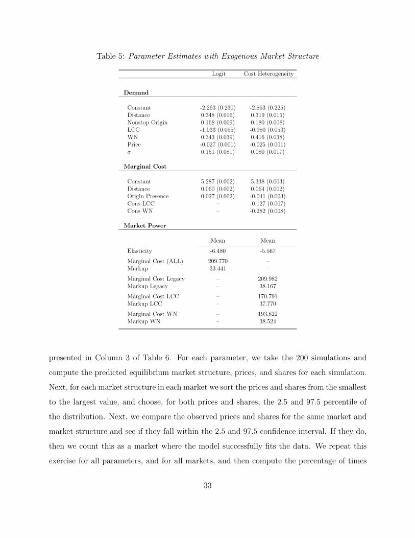
Table 5: Parameter Estimates with Exogenous Market Structure

Logit Cost Heterogeneity

Demand

Constant -2.263 (0.230) -2.863 (0.225)Distance 0.348 (0.016) 0.319 (0.015)Nonstop Origin 0.168 (0.009) 0.180 (0.008)LCC -1.033 (0.055) -0.980 (0.053)WN 0.343 (0.039) 0.416 (0.038)Price -0.027 (0.001) -0.025 (0.001)� 0.151 (0.081) 0.080 (0.017)

Marginal Cost

Constant 5.287 (0.002) 5.338 (0.003)Distance 0.060 (0.002) 0.064 (0.002)Origin Presence 0.027 (0.002) -0.041 (0.003)Cons LCC – -0.127 (0.007)Cons WN – -0.282 (0.008)

Market Power

Mean Mean

Elasticity -6.480 -5.567

Marginal Cost (ALL) 209.770 –Markup 33.441 –

Marginal Cost Legacy – 209.982Markup Legacy – 38.167

Marginal Cost LCC – 170.791Markup LCC – 37.770

Marginal Cost WN – 193.822Markup WN – 38.524

presented in Column 3 of Table 6. For each parameter, we take the 200 simulations and

compute the predicted equilibrium market structure, prices, and shares for each simulation.

Next, for each market structure in each market we sort the prices and shares from the smallest

to the largest value, and choose, for both prices and shares, the 2.5 and 97.5 percentile of

the distribution. Next, we compare the observed prices and shares for the same market and

market structure and see if they fall within the 2.5 and 97.5 confidence interval. If they do,

then we count this as a market where the model successfully fits the data. We repeat this

exercise for all parameters, and for all markets, and then compute the percentage of times

33

that the model fits the data. We find that we fit the prices 33 percent of the times, and the

shares 74 percent of the times. We find that we predict the market structure observed in

the data 16 percent of the times.

In Column 1 of Table 6 we estimate the coe�cient of price to be included in [-0.016,

-0.015] with a 95 percent probability, which is to be compared to the estimate of -0.027

(s.e. of 0.001) that we found in Column 1 of Table 5. The estimate in Table 6 is almost

twice as large in absolute value than the one in Table 5, and the di↵erence is even more

striking when we compare the price estimates in the Columns 2 of the two tables. This is an

important finding, which is consistent with the Monte Carlo exercise presented in Section C

of the Online Supplement. These results imply that not accounting for endogenous market

structure gives biased estimates of price elasticity.

Table 6: Parameter Estimates with Endogenous Market Structure

Baseline With Cost HeterogeneityUtilityConstant [-4.333, -4.299] [-5.499, -5.467]Distance [ 0.246, 0.256] [ 0.184, 0.191]Nonstop Origin [ 0.157, 0.163] [ 0.125, 0.130]LCC [-0.481, -0.401] [-0.345, -0.333]WN [ 0.016, 0.144] [ 0.222, 0.230]Price [-0.016, -0.015] [-0.012, -0.011]� [ 0.489, 0.508] [ 0.481, 0.499]

Marginal CostConstant [ 5.143, 5.368] [ 5.173, 5.221]Distance [-0.051, 0.013] [ 0.030, 0.031]Origin Presence [-0.180, -0.173] [-0.242, -0.233]LCC – [-0.132, -0.127]WN – [-0.088, -0.085]

Fixed CostConstant [ 7.726, 8.466] [ 7.768, 8.066]Nonstop Origin [-0.079, -0.015] [-0.142, -0.137]Nonstop Dest. [-0.456, -0.439] [-0.333, -0.321]LCC – [-0.003, -0.003]WN – [-1.642, -1.583]

Variance-CovarianceDemand Variance [ 1.898, 2.006] [ 1.510, 1.570]FC Variance [ 2.152, 2.240] [ 2.010, 2.086]Demand-FC Correlation [ 0.764, 0.795] [ 0.721, 0.758]Demand-MC Correlation [ 0.621, 0.709] [ 0.382, 0.396]MC-FC Correlation [ 0.030, 0.159] [-0.299, -0.288]

We estimate � in Column 1 of Table 5 equal to 0.151 (s.e. 0.081), while here in the

34

Column 1 of Table 6 it is included in [0.489,0.508]; and it is equal to 0.080 (0.017) in Column

2 of Table 5 and is included in [0.481,0.499] in Column 2 of Table 6. Thus, we find that the

within correlation is also estimated with a bias when we do not control for the endogenous

market structure. It is much larger in Table 6 than in Table 5.

Overall, these sets of results lead us to over-estimate the elasticity of demand and under-

estimate the market power of airline firms when we maintain that market structure is ex-

ogenous. To see this, observe that in Column 2 of Table 5 the (inferred) mean elasticity is

-5.567, which is consistent with previous estimates (e.g. Ciliberto and Williams, 2014). The

markup for legacy carriers is 38.167, the one for LCCs 37.770, and then one for Southwest

38.524 (0.848). In comparison, using our methodology the mean elasticity is included in

[-2.43,-2.40], and the markup for the legacy carriers is included in [52.44, 53.32], which is,

approximately, sixty percent larger (displayed in Table 7). Similarly, the markup for the

LCCs and WN are included, respectively, in [47.29,48.1] and [49.85,50.73].

The marginal cost estimates are also di↵erent between the exogenous entry and endoge-

nous entry specifications. In Table 5, we find the (mean) marginal cost equal to 209.982

for the legacy carriers, 170.791 for the LCCS, and 193.822 for WN. Because the markups

are larger in Table 7, the marginal costs will have to be smaller, which is exactly what we

find, as we estimate the mean of the marginal costs of the legacy carriers to be included in

[194.75,196.90], the one of LCCs in [158.15,160.13], and the one of WN in [174.25,176.68].

Next, we show the results for the estimates of the fixed cost equations. Clearly, these are

not comparable to the results from the previous model where market structure is assumed

to be exogenous.

Column 1 of Table 6 shows the constant in the fixed cost equation to be included in

[7.726,8.466], and the variables Nonstop Origin and Nonstop Destination to be negative, as

one would expect if there were economies of density. The results are similar in Column 2,

where the constant is included in [7.768,8.066], the coe�cient of Nonstop Origin in [-0.142,-

0.137], and the one of Nonstop Destination in [-0.333,-0.321]. In Column 2 we allow for

the LCCs to have a di↵erent constant, but do not find evidence of that, as the estimate

35

is included in [-0.003,-0.003]. The constant of WN is much smaller, as it is included in

[-1.642,-1.583].

Table 7: Market Power Estimates with Endogenous Market Structure

Confidence Interval

Own Elasticity of Demand [-2.43,-2.40]

Marginal Cost Legacy [194.75,196.90]Markup Legacy [51.25,53.40]

Marginal Cost LCC [158.15,160.13]Markup LCC [48.43,50.41]

Marginal Cost WN [174.25,176.68]Markup WN [55.67,58.09]

Finally, we investigate the estimation results for the variance-covariance matrix. The

variances are precisely estimated in both Columns, with the demand variance being included

in [1.898,2.006] in Column 1 and in [1.510,1.570] in Column 2. The variance of the fixed

cost unobservables is estimated in [2.152,2.240] in Column 1 and [2.010,2.086] in Column 2.

Recall that the variance of the marginal cost unobservables is normalized to its value from

the GMM estimation.

The correlation between the unobservables of the demand and fixed cost unobservables

is estimated to be included in [0.764,0.795] in Column 1 and in [0.721,0.758] in Column 2.

The correlation between the demand and marginal cost unobservables is also positive, as it

is included in [0.621,0.709] in Column 1 and in [0.382,0.396] in Column 2.27 This is one way

that self-selection manifests itself in the model, in the sense that firms that face higher fixed

costs are also the firms that are more likely to o↵er higher quality products.

These correlations imply that the unobservables that would, ceteris paribus, increase the

demand for a given good, are positively correlated with those that would increase the fixed

and marginal cost of producing that good. This makes intuitive sense if we think of the

unobservables as measuring quality, for example, and thus higher quality increases demand,

but it also increases the fixed and marginal costs, in the same spirit as Bresnahan (1987).

27These intervals are very tight, and much of the precision is due to our use of the additional momentsdescribed in Section 3.4.

36

The results for the correlation between the marginal and fixed costs unobservables are

di↵erent in Columns 1 and 2. They are positive and only marginally statistically di↵erent

from zero in Column 1, while they are negative in Column 2. Since Column 2 presents

the more flexible model, we will use it for our interpretation of the relationship between

the marginal and fixed cost unobservables. The negative relationship implies that there

is a potential trade o↵ between fixed and marginal costs unobservables. Continuing our

interpretation of the unobservables as unobserved quality, the negative correlation would

imply that the higher the fixed costs associated with producing a high quality good, the

lower the corresponding marginal costs.

6 The Economics of Mergers When Market Structure

is Endogenous

We present results from counterfactual exercises where we allow a merger between two firms,

American Airlines and US Air. A crucial concern of a merger from the point of view of

a competition authority is the change in prices after the merger. It is typically thought

that mergers imply greater concentration in a market which would imply an increase in

prices. Because of this concern with rising prices, the use of canonical models of product

di↵erentiation seems well suited to asses the impact of a merger. However, mergers may

also lead to cost e�ciencies, which would put downward pressure on prices. Also, a firm

may gain some technology that improves its demand, allowing it to enter a market that was

previously unprofitable. Because of these other consequences of a merger it is reasonable to

think that firms would make di↵erent optimal entry/exit decisions in response to a merger.

For example, if two firms become one in a particular market after their merger, there might

be room in the market for another entrant. Or if the merged firm inherits a better utility

characteristics in a particular market after the merger, it may be in a position to either enter

a new market, or price out a rival in an existing market.

Our methodology is ideally suited to evaluate both the price e↵ects of mergers like these

traditional studies, as well as the market structure e↵ects of mergers. Importantly, as we

37

discuss below, changes in market structure imply changes in prices, and viceversa, so in-

corporating optimal entry decisions into a merger analysis is crucial for understanding the

total e↵ect of mergers on market outcomes. In contrast, the canonical model of competition

among di↵erentiated products takes as exogenous the set of products competing (eg BLP

and Nevo, 2001).28

6.1 The Price and Market Structure E↵ects of the AA-US Merger

To begin with, for a particular market, if US Airways (US) was a potential entrant, we delete

them.29 If American is a potential entrant before the merger, they continue to be a potential

entrant after the merger. If American (AA) was not a potential entrant and US Air was a

potential entrant before the merger, we assume that after the merger American is a potential

entrant. If neither firm was a potential entrant before the merger, American continues to

not be a potential entrant after the merger.

Next, in the merger counterfactual that we perform, we consider the “best case” scenario

from the point of view of the merging firms. We look at the “best case” scenario with the

purpose of seeing if there would be any benefits under that most favorable scenario from the

viewpoint of the merging parties. If there were no (or limited) benefits under the merger in

our scenario, then it would be a strong case to argue against the merger.

Thus, to combine the characteristics of both firms, we assign the “best” characteristic

between AA and US to the new merged firm. For example, in the consumer utility function,

our estimate of “non-stop origin” is positive, so after the merger, we assign the maximum of

“non-stop origin” between AA and US to the post-merger AA. For marginal costs, we assign

the highest level of “origin presence” between AA and US to the post-merger AA. And for

fixed costs, we assign the highest level of “non-stop dest.” and “non-stop origin” between

AA and US to the post-merger AA. We do the same exact procedure for the unobserved

28Mazzeo et. al. (2014) make a similar argument. They quantify the welfare e↵ects of merger withendogenous enty/exit in a computational exercise using a stylized model that is similar to our model. Incontrast, we provide a methodology to estimate an industry model and perform a merger analysis usingthose estimates. Also, we allow for multiple equilibiria in both estimation and the merger analysis, whereasMazzeo et. al. (2014) assume a unique outcome from a selection rule based on ex ante firm profitability.

29In this merger, American is the surviving firm.

38

shocks. We use the same simulation draws from estimation for the merger scenario, and we

assign the “best” simulation draw (for utility the highest and for costs the lowest) between

AA and US to the post-merger AA.

In the following tables we report the likelihood of observing particular market structures

(sometimes conditional on the pre-merger market structure) and expected prices conditional

on a particular market structure transition. In all cases we report 95% confidence intervals

constructed using the procedure we used to construct intervals for inference on the parameters

in the model, the sub-sampling procedure in Chernozhukov, Hong, and Tamer (2007). Given

that we have already completed the sub-sampling for the parameter estimates, there is no

extra sampling that needs to be done to construct confidence intervals for our counterfactual

results. We run the counterfactual scenarios for 100 parameter vectors that are contained

in the original confidence region. For example, to attain the confidence interval for average

prices for a single firm across all markets, we would compute the statistic for each parameter

vector and then take 2.5 and 97.5 percentiles of these estimates, across the 100 parameter

vectors, as our confidence region.

We begin our analysis looking at two sets of markets: markets that were not served by

any airline before the merger and markets that were served by American and USAir as a

duopoly before the merger. This is a natural starting point because we want to ask whether,

as the consequence of the merger of American and USAir, new markets could be profitably

served, which is clearly a strong reason for the antitrust authorities to allow for a merger to

proceed. We also want to ask whether, as the consequence of the merger, markets that were

previously served only by the merging parties experience higher ticket prices.

Table 8 is a simple “transition” matrix that relates the probability of observing a mar-

ket structure post-merge (Columns) conditional on observing a market structure pre-merge

(Rows).30 The complete transition matrix would be of dimension 64 x 32, which we do not

present for practical purposes. Here we only present a 2 x 2 matrix, where the two pre-

merger market structures are those markets with no firm in the market and with a duopoly

30Although our model is static, we use the terminology “transition” in order to convey predicted changespre-merger to post-merger.

39

of US and AA; and the post-merger market structures are those markets with no firm in the

market and with a monopoly of AA/US.

Table 8 shows that conditional on observing a market with no firms pre-merge, the prob-

ability of observing the market not being served post-merge is between 36 and 90 percent. If

the market was an American and USAir duopoly pre-merger, there is a probability between

20 and 82 percent that the market will now be served by the merged firm. The probability

that the merged firm AA/US will enter a market that was not previously being served is

between 10 and 19 percent, which is a substantial and positive e↵ect of the merger.

Table 8: Market Structures in AA and US Monopoly and Duopoly Markets

Post-merger

Pre-merger No Firms AA Monopoly

No Firms [0.36,0.90] [0.10,0.19]AA/US Duopoly [0.00,0.01] [0.20,0.82]

We find (result not in the tables) that in markets where American and USAir were in a

duopoly and now act as a monopolist the prices are unchanged (the confidence interval is

equal to [0.00,0.01]). There are at least three explanations for this result. First, this might

be a result driven by the fact that we are averaging across many di↵erent markets, and there

might be some where the increase in prices was substantial. Second, it might be the case that

American and USAir were already tacitly colluding, and thus the price could only go down

after the two firms as they would exploit any cost e�ciencies available to them. Finally,

it might be the case that the cost e�ciencies were so substantial that any increase in price

was o↵set by the cost gains. We explore the first explanation in detail later. Determining

whether the firms were tacitly colluding pre-merger is beyond the scope of this paper, and

we refer the reader to Ciliberto and Williams [2014] for an investigation on tacit collusion

in the airline industry. We will discuss the nature of the cost savings from the mergers in

detail later.

An argument that is made to allow for the merger of two firms looks at the markets

where the merging parties are the only firms in the market, and then studies whether there

40

is a potential entrant who would enter if the merging parties were to raise their prices as

a consequence of their merger. Table 9 considers the probability that one of the other

four competitors will enter into the market where there was a duopoly of American and

USAir pre-merger. We find that Delta will enter with a probability included between 8 and

25 percent, which clearly suggest that there is a substantial possibility that Delta enters,

with the consequence of limiting the market power of the new merged airline. We also find

evidence that United, and, to a lesser extent, LCC and WN will enter after the merger in a

market that would otherwise be a monopoly of AA/US.

Table 9: Entry of Competitors in AA and US Duopoly Markets

Prob mkt structure Duopoly AA/US & DL Duopoly AA/US & LCC Duopoly AA/US & UA Duopoly AA/US & WN

Duopoly AA & US [0.08,0.25] [0.01,0.02] [0.05,0.11] [0.00,0.01]

We can now investigate how the entry of the other potential entrants would change the

prices in those markets that were AA and US duopolies pre-merger. We find that the

prices would drop when DL enters into the market, by a percentage included in [-0.12,-

0.01], and when United enters, by a percentage included in [-0.06,0.00]. There would not

be a statistically significant change in the prices when LCC enters, while there would be an

increase in the prices when WN enters. We interpret these results as suggesting that DL

and UA o↵er a service that is a closer substitute to the one provided by AA and US than

WN and LCC do.

Table 10: Prices of Competitors in AA and US Duopoly Markets

Change in the price of AA Duopoly AA/US & DL Duopoly AA/US & LCC Duopoly AA/US & UA Duopoly AA/US & WN

Duopoly AA & US [-0.12,-0.01] [-0.01,0.03] [-0.06,0.00] [0.00,0.04]

We now take a di↵erent direction of investigation. Instead of focusing on markets where

there would be an ex-ante concern that prices increase after the merger, we explore in more

depth the possible benefits of a merger, which could allow a new, possibly more e�cient,

firm to enter into new markets.

In Table 11 we consider the likelihood of entry of AA after its merger with US in markets

41

where American was not present pre-merger, but is present post-merger. In this table we

only consider a selected set of scenarios, which we chose as they appear most frequently in

the data. In Columns 1 and 2 we consider the cases when the pre-merger market structure is

a monopoly and AA enters to replace the pre-merger monopolist (Column 1), or adds itself

to form a duopoly (Column 2). In Column 3 we present the case when AA enters to add

itself to a duopoly, thus generating a triopoly market. In Columns 4 and 5 display the cases

when the market structure changes, respectively, from a triopoly to quadropoly, and from a

quadropoly to a quintopoly.

The first row of Column 1 shows that, conditional on observing a monopoly of Delta

before the merger, we will predict that American/USAir would replace Delta with a prob-

ability between 2 and 9 percent. Conditional on observing a monopoly of a LCC before

the merger, we observe American replacing the LCC with a probability between 7 and 19

percent. Overall, there is clear evidence that AA/US will replace some of the other carriers

as monopolist.

The first row of Column 2 shows that, conditional on Delta being a monopoly pre-merger,

American is likely to enter, post-merger, with a probability between 19 and 25 percent.

This is larger, in a way that is statistically significant, than what we had found in Column

1. Similarly, we find the probabilities that AA enters to form a duopoly with United and

Southwest to be larger than AA replacing them as a monopolist. This provides evidence

that markets may actually become less concentrated after a merger because of the optimal

entry decision of the merged firms.

Table 11: Post-merger Entry of AA in New Markets

(1) (2) (3) (4) (5)Monopoly Duopoly 3-opoly 4-opoly

Pre-merger AA AA Pre-merger AA Pre-merger AA Pre-merger AAFirms Replacement Entry Firms Entry Firms Entry Firms Entry

DL [0.02,0.09] [0.19,0.25] DL,LCC [0.09,0.27] DL,LCC,UA [0.21,0.35] DL,LCC,UA,WN [0.27,0.44]LCC [0.07,0.19] [0.02,0.14] DL,UA [0.24,0.32] DL,LCC,WN [0.10,0.33]UA [0.04,0.12] [0.10,0.21] DL,WN [0.16,0.27] DL,UA,WN [0.29,0.37]WN [0.01,0.04] [0.10,0.19] LCC,UA [0.05,0.22] LCC,UA,WN [0.07,0.29]

LCC,WN [0.04,0.23]UA,WN [0.11,0.26]

42

The first row of Column 3 shows that, conditional on observing a duopoly of DL and

UA, American is likely to enter and form a triopoly with a probability between 24 and 32

percent. Columns 4 and 5 present results that show that the probability that American

enters post-merger is generally increasing in the number of firms that are in the market

pre-merger, though there is some considerable heterogeneity depending on the identity of

the firms that were in the market pre-merger.

We can now proceed to see how prices would change after the entry of AA in a market.

Clearly, we can only construct price changes for firms that were in the market pre- and

post-merger. So, for example, we do not have a change in price in markets where AA/US

replaces DL. For markets where AA/US enters to form a duopoly with Delta, we will have

the change in prices for DL, but not for AA/US. In Table 12, we present the price changes

under di↵erent scenarios. The scenarios presented in Columns 1, 2, 3, and 4 of Table 12

correspond, respectively, the the ones in Columns 2, 3, 4, and 5 of Table 11.

The first row of Column 1 in Table 12 shows that the price of the median ticket on a

flight with DL drops between by between 8 and 12 percent when American enters to form a

duopoly. The results are quite similar when we look at the e↵ect of AA/US’s entry on the

prices of the other competitors. The first row of Column 2 in Table 12 shows that the e↵ect

on the prices of the entry of American are smaller when the original market structure was

a duopoly, and this is true for any of the duopolies we consider. The results in Columns 3

and 4 show that the entry of American has an increasingly smaller e↵ect on the prices of the

incumbent oligopolists as their number increases.

The intuition for why AA/US enters new markets and the corresponding change in prices

is straightforward. Under our assumptions about the merger, the new firm will typically

have higher utility and/or lower costs in any given market than each of AA and US did

separately before the merger. Low costs will promote entry of AA and lower prices for rivals

after entry (in our model prices are strategic complements) and higher utility will promote

entry by AA and upward price pressure, or even lead to exit by incumbents, as we see in

those monopoly markets where AA/US replaces the incumbent.

43

Table 12: Post-Merger Price Changes After the Entry of AA in New Markets

Monopoly Duopoly 3-opoly 4-opoly

Pre-merger Pre-merger Pre-merger Pre-mergerFirms %�Price Firms %�Price Firms %�Price Firms %�Price

DL [-0.12,-0.08] DL [-0.05,-0.03] DL [-0.03, -0.01] DL [-0.02, -0.01]LCC [-0.01,-0.01] LCC [-0.01,-0.00] LCC [-0.00,-0.00]

UA [-0.015 -0.010] UA [-0.01,-0.01]WN [-0.01,-0.00]

LCC [-0.10,-0.09] DL [-0.04,-0.02] DL [-0.028,-0.014]UA [-0.02,-0.02] LCC [-0.008,-0.004]

WN [-0.012,-0.008]

UA [-0.12,-0.09] DL [-0.05,-0.03] DL [-0.021,-0.013]WN [-0.02,-0.01] UA [-0.016,-0.010]

WN [-0.008,-0.006]

WN [-0.11,-0.08] LCC [-0.02,-0.01] LCC [-0.011,-0.005]UA [-0.04,-0.03] UA [-0.025,-0.015]

WN [-0.009,0.001]

LCC [-0.04,-0.02]WN [-0.05,-0.02]

UA [-0.04,-0.03]WN [-0.02,-0.02]

Table 13 focuses on markets where AA is already present in the market and another in-

cumbent exits after the merger. This is clearly di↵erent than what we have just investigated,

where (the new) AA was simply adding itself into a market, and the consumers would clearly

benefit, generally with lower prices and greater product variety. There are two reasons why

a competitor would drop out of a market after a merger. First, after the merger AA might

become more e�cient in terms of costs, lowers the prices, and and now a rival cannot make

enough variable profit to cover fixed costs.31 Second, AA might become more attractive to

consumers after the merger and steal business from rivals. For ease of exposition we only

considers markets where AA and other incumbents were in the market, and we do not report

the results for the other merging firm, USAir.

The first row of Column 1 in Table 13 shows that there is a probability between 3 and 5

percent that DL will leave the duopoly market with AA after American merges with USAir.

31AA could either experience a decrease in marginal costs, or a decrease in fixed costs. For the fixed costscase, AA could have been a low marginal costs firm before the merger, but high fixed costs prevented entry.After the merger an decrease in fixed costs could lead to entry with the already low marginal costs.

44

The second row shows that the probability that a LCC exits the (duopoly) market is much

larger, between 9 and 16 percent. United and Southwest exit the market with a proba-

bility, respectively, included in [0.06,0.08] and [0.02,0.05]. These are all economically and

statistically significant probabilities, and provide another piece of evidence that the AA/US

merger has complex e↵ects, ranging well beyond the typical analysis that is circumscribed

to markets where the merging parties are pre-merger duopolies.

Table 13: Likelihood of Exit by Competitors after AA-US Merger

Duopoly with AA 3-opoly with AA

Pre-merger Pre-mergerFirm Exit Firms Exit

DL [0.03,0.05] DL [0.05,0.15]LCC [0.01,0.01]

LCC [0.09,0.16] DL [0.04,0.14]UA [0.01,0.05]

UA [0.06,0.08] DL [0.02,0.03]WN [0.02,0.05]

WN [0.02,0.05] LCC [0.02,0.03]UA [0.05,0.12]

LCC [0.00,0.02]WN [0.07,0.11]

UA [0.01,0.03]WN [0.03,0.05]

Next, in Table 14 we consider what happens to prices after markets become more concen-

trated after the merger. We observe that, with the exception of Delta, all the price changes

in the first Column of Table 14 are positive. For example, after the exit of a LCC in a

AA-LCC duopoly, American (now a monopolist) would increase its price by a percentage

included between 1 and 7 percent (Row 2, Column 1). This result makes sense to the extent

that now American is a monopoly, while pre-merger it was a duopoly. However, it may

surprising that American can increase its prices and the LCC decides to exit. One would

think that the profit of the LCC would increase as American increases its prices, and that

would make the LCC less likely to exit the market. The key to understand this apparent

paradox is that, under the best scenario, American is not only incurring lower costs, but it

is also facing a stronger demand for its product, which comes at the cost of its competitors

45

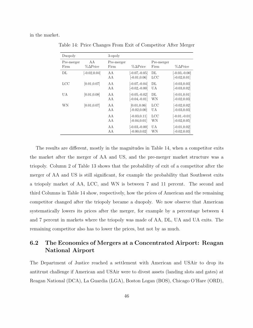
in the market.

Table 14: Price Changes From Exit of Competitor After Merger

Duopoly 3-opoly

Pre-merger AA Pre-merger Pre-mergerFirm %�Price Firm %�Price Firm %�Price

DL [-0.02,0.04] AA [-0.07,-0.05] DL [-0.03,-0.00]AA [-0.01,0.06] LCC [-0.02,0.01]

LCC [0.01,0.07] AA [-0.07,-0.04] DL [-0.03,0.03]AA [-0.02,-0.00] UA [-0.03,0.02]

UA [0.01,0.08] AA [-0.05,-0.02] DL [-0.01,0.01]AA [-0.04,-0.01] WN [-0.02,0.03]

WN [0.01,0.07] AA [0.01,0.06] LCC [-0.02,0.02]AA [-0.02,0.00] UA [-0.03,0.03]

AA [-0.03,0.11] LCC [-0.01,-0.01]AA [-0.04,0.01] WN [-0.02,0.05]

AA [-0.03,-0.00] UA [-0.01,0.02]AA [-0.00,0.02] WN [-0.02,0.03]

The results are di↵erent, mostly in the magnitudes in Table 14, when a competitor exits

the market after the merger of AA and US, and the pre-merger market structure was a

triopoly. Column 2 of Table 13 shows that the probability of exit of a competitor after the

merger of AA and US is still significant, for example the probability that Southwest exits

a triopoly market of AA, LCC, and WN is between 7 and 11 percent. The second and

third Columns in Table 14 show, respectively, how the prices of American and the remaining

competitor changed after the triopoly became a duopoly. We now observe that American

systematically lowers its prices after the merger, for example by a percentage between 4

and 7 percent in markets where the triopoly was made of AA, DL, UA and UA exits. The

remaining competitor also has to lower the prices, but not by as much.

6.2 The Economics of Mergers at a Concentrated Airport: ReaganNational Airport

The Department of Justice reached a settlement with American and USAir to drop its

antitrust challenge if American and USAir were to divest assets (landing slots and gates) at

Reagan National (DCA), La Guardia (LGA), Boston Logan (BOS), Chicago O’Hare (ORD),

46

Dallas Love Field (DAL), Los Angeles (LAX), and Miami International (MIA) airports. The

basic tenet behind this settlement was that new competitors would be able to enter and

compete with AA and US, should the new merged airline significantly rise prices.

Here, we conduct a counter-factual on the e↵ect of the merger in markets originating

or ending at DCA. These markets were of the highest competitive concern for antitrust

authorities because both merging parties had a very strong incumbent presence.

Table 15 reports the results of a counterfactual exercise that looks at the entry of new

competitors and at the price changes in markets with DCA as an endpoint that were AA

and US duopoly before the merger. The first row shows that there is a probability included

between 16.1 and 71 percent that there will be a AA monopoly post-merger. There is a

probability between 13.6 and 22.7 percent that Delta will enter into the market after AA

and US merge. United is also likely to enter into these markets, with a probability included

between 5.9 and 18.8 percent. The probability that a LCC or WN enters into the market is

negligible.

The second row reports the price changes predicted under the new market structure. Most

crucially, we observe that the prices increase by a percentage included between 1.9 and 8.9

percent when AA is the post-merger monopolist. This is the first, strong, piece of evidence

that the AA and US merger would provide localized market power in important geographical

markets, even under the ”best” case scenario for the merging parties. When a competitor

enters, the prices changes are not statistically di↵erent from zero, suggesting that new entry

does limit the market power gained through a merger.

Overall, our results suggest that the decisions made by the Department of Justice to

facilitate the access to airport facilities to new entrants were well justified, and should help

controlling the post-merger increase in prices.

Table 15: Post-merger entry and pricing in pre-merger AA & US Duopoly markets, ReaganNational Airport

Prob mkt structure Monopoly AA/US Duopoly AA/US & DL Duopoly AA/US & LCC Duopoly AA/US & UA Duopoly AA/US & WN

Mkt Struct. Transitions [0.161, 0.710] [ 0.136, 0.227] [0.000, 0.047] [0.059, 0.188] [0.000, 0.000]% Change in Prices [0.019, 0.089] [-0.095, 0.018] [-0.073, 0.126] [-0.114, 0.068] [n.a.]

47

7 Conclusions

We provide an empirical framework for studying the quantitative e↵ect of self-selection of

firms into markets and its e↵ect on market power in static models of competition. The coun-

terfactual exercises consist of merger simulation that allow for changes in market structures,

and not just in prices. The main takeaways are: i) that self-selection occurs and controlling

for it can lead to di↵erent estimates of price elasticities and markups than those that we

find when we assume that market structure is exogenous to the pricing decision.; ii) this

in turn leads to potentially important responses to policy counterfactuals such as merger

simulations.

More generally, this paper contributes to the literature that studies the e↵ects that merg-

ers or other policy changes have on the prices and structure of markets, and consequently

the welfare of consumers and firms. These questions are of primary interest for industrial

organization economists, both academics and researchers involved in antitrust and policy

activities.

One extension of our model is to a context where firms can change the characteristics of

the products they o↵er. To illustrate, consider Goeree (2008) who investigates the role of

informative advertising in a marketwith limited consumer information. Goeree (2008) shows

that the prices charged by producers of personal computers would be higher if firms did not

advertise their products because consumers would be unaware of all the potential choices

available to them, thus granting greater market power to each firm. However, this presumes

that the producers would continue to optimally produce the same varieties if consumers

were less aware, while in fact one would expect them to change the varieties available if

consumers had less information, for example by o↵ering less di↵erentiated products. It is

possible to extend our framework to investigate questions like this where firms choose product

characteristics.

Finally, the proposed methodology can be applied in all economic contexts where agents

interact strategically and make both discrete and continuous decisions. For example, it can

be applied to estimate a model of household behavior where a husband and a wife must

48

decide whether to work and how many hours.

49

References

Berry, Steven and Panle Jia. 2010. “Tracing the Woes: An Empirical Analysis of the Airline

Industry.” American Economic Journal: Microeconomics 2 (3):1–43.

Berry, Steven, James Levinsohn, and Ariel Pakes. 1995. “Automobile prices in market

equilibrium.” Econometrica: Journal of the Econometric Society :841–890.

Berry, Steven T. 1990. “Airport presence as product di↵erentiation.” The American Eco-

nomic Review :394–399.

———. 1992. “Estimation of a Model of Entry in the Airline Industry.” Econometrica:

Journal of the Econometric Society :889–917.

———. 1994. “Estimating discrete-choice models of product di↵erentiation.” The RAND

Journal of Economics :242–262.

———. 1999. “Free entry and social ine�ciency in radio broadcasting.” The RAND Journal

of Economics 30 (3):397–420.

Bresnahan, Timothy F. 1987. “Competition and collusion in the American automobile in-

dustry: The 1955 price war.” The Journal of Industrial Economics :457–482.

———. 1989. “Empirical studies of industries with market power.” Handbook of industrial

organization 2:1011–1057.

Bresnahan, Timothy F and Peter C Reiss. 1990. “Entry in monopoly market.” The Review

of Economic Studies 57 (4):531–553.

———. 1991. “Entry and competition in concentrated markets.” Journal of Political Econ-

omy :977–1009.

Brueckner, Jan K and Pablo T Spiller. 1994. “Economies of tra�c density in the deregulated

airline industry.” Journal of Law and Economics :379–415.

50

Chernozhukov, Victor, Han Hong, and Elie Tamer. 2007. “Estimation and confidence regions

for parameter sets in econometric models1.” Econometrica 75 (5):1243–1284.

Ciliberto, Federico, Amalia Miller, Helena Skyt Nielsen, and Marianne Simonsen. 2010.

“Playing the fertility game at work.” Unpublished manuscript .

Ciliberto, Federico and Elie Tamer. 2009. “Market structure and multiple equilibria in airline

markets.” Econometrica 77 (6):1791–1828.

Ciliberto, Federico and Jonathan W Williams. 2014. “Does Multimarket Contact Facilitate

Tacit Collusion? Inference on Conduct Parameters in the Airline Industry.” Inference on

Conduct Parameters in the Airline Industry (February 12, 2014) .

Cohen, Andrew M and Michael J Mazzeo. 2007. “Market structure and competition among

retail depository institutions.” The Review of Economics and Statistics 89 (1):60–74.

Draganska, Michaela, Michael Mazzeo, and Katja Seim. 2009. “Beyond plain vanilla: Mod-

eling joint product assortment and pricing decisions.” QME 7 (2):105–146.

Eizenberg, Alon. 2014. “Upstream Innovation and Product Variety in the US Home PC

Market*.” The Review of Economic Studies :rdu004.

Elzinga, Kenneth G and David E Mills. 2009. “Predatory Pricing in the Airline Industry:

Spirit Airlines v. Northwest Airlines (2005).” The Antitrust Revolution, 5th Edition, edited

by J. Kwoka and L. White, Forthcoming .

Goeree, Michelle Sovinsky. 2008. “Limited information and advertising in the US personal

computer industry.” Econometrica 76 (5):1017–1074.

Goolsbee, Austan and Chad Syverson. 2008. “How Do Incumbents Respond to the Threat

of Entry? Evidence from the Major Airlines.” The Quarterly Journal of Economics

123 (4):1611–1633.

51

Gronau, Reuben. 1974. “Wage Comparisons–A Selectivity Bias.” The Journal of Political

Economy :1119–1143.

Heckman, James J. 1976. “The common structure of statistical models of truncation, sample

selection and limited dependent variables and a simple estimator for such models.” In

Annals of Economic and Social Measurement, Volume 5, number 4. NBER, 475–492.

———. 1979. “Sample selection bias as a specification error.” Econometrica: Journal of the

econometric society :153–161.

Ho, Katherine. 2008. “Insurer-Provider Networks in the Medical Care Market.” American

Economic .

Mazzeo, Michael J. 2002. “Product choice and oligopoly market structure.” RAND Journal

of Economics :221–242.

Nevo, Aviv. 2000. “Mergers with di↵erentiated products: The case of the ready-to-eat cereal

industry.” The RAND Journal of Economics :395–421.

Pakes, Ariel, J Porter, Joy Ishii, and Kate Ho. 2015. “Moment Inequalities and Their

Application.” Econometrica 83:315–334.

Panzar, John C. 1979. “Equilibrium and welfare in unregulated airline markets.” The

American Economic Review :92–95.

Reiss, Peter C and Pablo T Spiller. 1989. “Competition and entry in small airline markets.”

Journal of Law and Economics :S179–S202.

Roberts, Jimmy and Andrew Sweeting. 2014. “The Potential Entry Defense in Airline Merg-

ers.” working paper, Duke University .

Rosse, James N. 1970. “Estimating cost function parameters without using cost data: Illus-

trated methodology.” Econometrica: Journal of the Econometric Society :256–275.

52

Schmalensee, Richard. 1989. “Inter-industry studies of structure and performance.” Hand-

book of industrial organization 2 2.

Seim, Katja. 2006. “An empirical model of firm entry with endogenous product-type choices.”

RAND Journal of Economics :619–640.

Tamer, Elie. 2003. “Incomplete simultaneous discrete response model with multiple equilib-

ria.” The Review of Economic Studies 70 (1):147–165.

53