Market Structure and Multiple Equilibria in Airline Marketsmshum/gradio/papers/ecta5368.pdf · market structure and multiple equilibria in airline markets ... market structure and

http://www.econometricsociety.org/

Econometrica, Vol. 77, No. 6 (November, 2009), 1791–1828

MARKET STRUCTURE AND MULTIPLE EQUILIBRIAIN AIRLINE MARKETS

FEDERICO CILIBERTOUniversity of Virginia, Charlottesville, VA 22903, U.S.A.

ELIE TAMERNorthwestern University, Evanston, IL 60208, U.S.A.

The copyright to this Article is held by the Econometric Society. It may be downloaded,printed and reproduced only for educational or research purposes, including use in coursepacks. No downloading or copying may be done for any commercial purpose without theexplicit permission of the Econometric Society. For such commercial purposes contactthe Office of the Econometric Society (contact information may be found at the websitehttp://www.econometricsociety.org or in the back cover of Econometrica). This statement mustthe included on all copies of this Article that are made available electronically or in any otherformat.


Econometrica, Vol. 77, No. 6 (November, 2009), 1791–1828

MARKET STRUCTURE AND MULTIPLE EQUILIBRIAIN AIRLINE MARKETS

BY FEDERICO CILIBERTO AND ELIE TAMER1

We provide a practical method to estimate the payoff functions of players in com-plete information, static, discrete games. With respect to the empirical literature onentry games originated by Bresnahan and Reiss (1990) and Berry (1992), the mainnovelty of our framework is to allow for general forms of heterogeneity across playerswithout making equilibrium selection assumptions. We allow the effects that the entryof each individual airline has on the profits of its competitors, its “competitive effects,”to differ across airlines. The identified features of the model are sets of parameters(partial identification) such that the choice probabilities predicted by the econometricmodel are consistent with the empirical choice probabilities estimated from the data.

We apply this methodology to investigate the empirical importance of firm hetero-geneity as a determinant of market structure in the U.S. airline industry. We find evi-dence of heterogeneity across airlines in their profit functions. The competitive effectsof large airlines (American, Delta, United) are different from those of low cost carri-ers and Southwest. Also, the competitive effect of an airline is increasing in its airportpresence, which is an important measure of observable heterogeneity in the airline in-dustry. Then we develop a policy experiment to estimate the effect of repealing theWright Amendment on competition in markets out of the Dallas airports. We find thatrepealing the Wright Amendment would increase the number of markets served out ofDallas Love.

KEYWORDS: Entry models, inference in discrete games, multiple equilibria, partialidentification, airline industry, firm heterogeneity.

1. INTRODUCTION

WE PROVIDE A PRACTICAL METHOD to estimate the payoff functions of playersin complete information, static, discrete games. With respect to the empiricalliterature on entry games originated by Bresnahan and Reiss (1990) (BR) andBerry (1992), the main novelty of our framework is to allow for general formsof heterogeneity across players without making equilibrium selection assump-tions. These assumptions are typically made on the form of firm heterogene-ity to ensure that, for a given value of the exogenous variables, the economicmodel predicts a unique number of entrants. In the ensuing econometric mod-els, multiple equilibria in the identity of the firms exist, but the number of en-trants is unique across equilibria. This uniqueness leads to standard estimation

1We thank a co-editor and three referees for comments that greatly improved the paper. Wealso thank T. Bresnahan, A. Cohen, B. Honoré, C. Manski, M. Mazzeo, A. Pakes, J. Panzar,A. Paula, R. Porter, W. Thurman, and seminar participants at many institutions and meetings forcomments. We especially thank K. Hendricks for insightful suggestions. We also thank S. Sakatafor help with a version of his genetic algorithm, Ed Hall for computing help, and T. Whalen atthe Department of Justice for useful insights on airlines’ entry decisions. B. Karali provided ex-cellent research assistance. The usual disclaimer applies. Tamer gratefully acknowledges researchsupport from the National Science Foundation and the A. P. Sloan Foundation.

© 2009 The Econometric Society DOI: 10.3982/ECTA5368



http://dx.doi.org/10.3982/ECTA5368

1792 F. CILIBERTO AND E. TAMER

of the parameter using maximum likelihood or method of moments. On theother hand, models with general forms of player heterogeneity have multipleequilibria in the number of entrants, and so the insights of BR and Berry donot generalize easily.

We present an econometric framework that allows for multiple equilibriaand where different selection mechanisms can be used in different markets.This framework directs the inferential strategy for a “class of models,” eachof which corresponds to a different selection mechanism. We use the simplecondition that firms serve a market only if they make nonnegative profits inequilibrium to derive a set of restrictions on regressions.2 In games with multi-ple equilibria, this simple condition leads to upper and lower bounds on choiceprobabilities.3 The economic model implies a set of choice probabilities whichlies between these lower and upper bounds. Heuristically, our estimator then isbased on minimizing the distance between this set and the choice probabilitiesthat can be consistently estimated from the data. Our econometric methodol-ogy restricts the parameter estimates to a set and thus partially identifies theparameters (see footnote 3). Each parameter in this set corresponds to a par-ticular selection mechanism that is consistent with the model and the data.We use recently developed inferential methods in Chernozhukov, Hong, andTamer (2007) (CHT) to construct confidence regions that cover the identifiedparameter with a prespecified probability.4

We apply our methods to data from the airline industry, where each obser-vation is a market (a trip between two airports).5 The idea behind cross-sectionstudies is that in each market, firms are in a long-run equilibrium. The objec-tive of our econometric analysis is to infer long-run relationships between theexogenous variables in the data and the market structure that we observe atsome point in time, without trying to explain how firms reached the observed

2The idea of deriving results for a class of models goes back to Sutton (2000). Taking a class ofmodels approach to game theoretic settings, one “abandon(s) the aim of identifying some uniqueequilibrium outcome. Instead, we admit some class of candidate models (each of which may haveone or more equilibria) and ask whether anything can be said about the set of outcomes that canbe supported as an equilibrium of any candidate model.” The necessary and weak condition onbehavior is similar to the “viability condition” discussed by Sutton (see also Sutton (1991)).

3Tamer (2003) also used this insight to show that, for a simple 2 ! 2 game with multipleequilibria, the model provides inequality restrictions on the regression. Sufficient conditions arethen given to guarantee that these inequality restrictions point-identify the parameter of interest.These conditions are not easy to generalize to larger games. However, the paper noted that, ingeneral, inequality restrictions constrain the parameter vector to lie in the identified set, and anestimator was suggested (Tamer (2003, p. 153)).

4CHT focused on constructing confidence regions for the arg min of a function (in this paper,the minimum distance objective function) and also confidence regions for the true but potentiallypartially identified parameter. Other econometric methods that can be used are Romano andShaikh (2008), Bugni (2007), Beresteanu and Molinari (2008), Andrews and Soares (2009), andCanay (2007).

5Berry (1992) used the same data source, but from earlier years.

MARKET STRUCTURE AND MULTIPLE EQUILIBRIA 1793

equilibrium. For example, we model the entry decision of American Airlinesas having a different effect on the profit of its competitors than the entry ofDelta or of low cost carriers has. In addition, we perform a policy exercise us-ing our estimated model to study how the Wright Amendment, a law restrict-ing competition in markets out of Dallas Love airport, affects the state of thesemarkets with respect to competition or market structure. This law was partiallyrepealed in 2006, so we can compare the predictions of our model with whatactually happened.

We estimate two versions of a static complete information entry game. Theseversions differ in the way in which the entry of a firm, its “competitive effect,”affects the profits of its competitors. In the simpler version, which follows theprevious literature, these competitive effects are captured by firm-specific in-dicator variables in the profit functions of other airlines. These indicator vari-ables measure the firms’ “fixed competitive effects.” In the more complex ver-sion, a firm’s competitive effect is a variable function of the firm’s measure ofobservable heterogeneity. The measure of observable heterogeneity that af-fects competitors’ profits is an airline’s airport presence, which is a functionof the number of markets served by a firm out of an airport. The theoreticalunderpinnings for these “variable competitive effects” are given in Hendricks,Piccione, and Tan (1997), who showed that as long as an airline has a large air-port presence, its dominant strategy is not to exit from a spoke market, even ifthat means it suffers losses in that market. Thus, the theoretical prediction isthat the larger an airline’s airport presence, the larger its variable competitiveeffects should be.

We find evidence of heterogeneity across airlines in their profit functions. Wefind that the competitive effects of large airlines (American, Delta, United) aredifferent from those of low cost carriers and Southwest. We also find that the(negative) competitive effect of an airline is increasing in its airport presence,which is an important measure of observable heterogeneity in the airline indus-try. Moreover, we also find evidence of heterogeneity in the effects of controlvariables on the profits of airline firms, which affects the probability of observ-ing different airlines as the control variables change. Then we develop a policyexperiment to estimate the effect of repealing the Wright Amendment on com-petition in markets out of the Dallas airports. We find that repealing the WrightAmendment would increase the number of markets served out of Dallas Love.As part of our analysis, we also estimate the variance–covariance matrix, andfind evidence of correlation in the unobservables as well as evidence of differ-ent variances and distributions of the firm unobservable heterogeneity.

This paper contributes to a growing literature on inference in discretegames. In the complete information setting, complementary approaches in-clude Bjorn and Vuong (1985) and Bajari, Hong, and Ryan (2005), where equi-librium selection assumptions are imposed. Another approach makes informa-tional assumptions. For example, Seim (2002), Sweeting (2004), and Aradillas-Lopez (2005) considered the case where the entry game has incomplete infor-mation, so that neither the firms nor the econometrician observe the profits of


all competitors. Andrews, Berry, and Jia (2003) proposed methods applicableto entry models to construct confidence regions for models with inequality re-strictions. More recently, Pakes, Porter, Ho, and Ishii (2005) provided a noveleconomic framework that leads to a set of econometric models with inequalityrestrictions on regressions. They also provide a method for obtaining confi-dence regions. Finally, further insights about identification in these settings isgiven in Berry and Tamer (2006).

This article also adds to the literature on inference in partially iden-tified models. This literature has a history in econometrics, starting withthe Frisch bounds on parameters in linear models with measurement error(Frisch (1934)) and the work of Marschak and Andrews (1944) (which con-tains one of the earliest examples of a structural model with partially identifiedparameters). More recently, Manski and collaborators further developed thisliterature with new results and made it part of the econometrics toolkit startingwith Manski (1990). See also Manski (2007) and the references therein, Manskiand Tamer (2002), and Imbens and Manski (2004). In the industrial organiza-tion literature, Haile and Tamer (2003) used partial identification methods toconstruct bounds on valuation distributions in second price auctions. In thestatistics literature, the Frechet bounds on joint distributions given knowledgeof marginals are well known (see also Heckman, Lalonde, and Smith (1999)),and these were used starting with the important result of Peterson (1976) incompeting risks. In the labor literature, the bounds approach to inference hasbeen prominent in the treatment–response and selection literature where sev-eral papers discuss and use exclusion restrictions to tighten the bounds andgain more information. See Manski (1994) for a discussion of the selectionproblem using partial identification and exclusion restrictions, and Blundell,Gosling, Ichimura, and Meghir (2007) and Honoré and Lleras-Muney (2006)for important empirical papers that use and expand this methodology. Seealso bounds based on revealed preference in Blundell, Browning, and Craw-ford (2003), and bounds on various treatment effects derived in Heckman andVytlacil (1999).

The remainder of the paper is organized as follows. Section 2 presents theempirical model of market structure and the main idea of the econometricmethodology. Section 3 formalizes the inferential approach, providing condi-tions for the identification and estimation of the parameter sets. Then Section 4discusses market structure in U.S. airline markets. Section 5 presents the esti-mation results. Section 6 reports the results of our policy experiment. Section 7concludes, and provides limitations and future work.

2. AN EMPIRICAL MODEL OF MARKET STRUCTURE

We follow Berry (1992) in modeling market structure. In particular, let theprofit function for firm i in market m be !im("; y"im), where y"im is a vector thatrepresents other potential entrants in market m and " is a finite parameter


of interest determining the shape of !im. This function can depend on bothmarket-specific and firm-specific variables.6

A market m is defined by Xm, where Xm = (Sm#Zm#Wm). Sm is a vectorof market characteristics which are common among the firms in market m;Zm = (Z1m# $ $ $ #ZKm) is a matrix of firm characteristics that enter into theprofits of all the firms in the market, for example, some product attributesthat consumers value; K is the total number of potential entrants in mar-ket m; Wm = (W1m# $ $ $ #WKm) are firm characteristics where Wim enters onlyinto firm i’s profit in market m, such as the cost variables.

The profit function for firm i in market m is

!im = S#m%i +Z#

im&i +W #im'i +

!

j $=i

(ijyjm +!

j $=i

Z#jm)

ijyjm + *im#(1)

where *im is the part of profits that is unobserved to the econometrician.7 Weassume throughout that *im is observed by all players in market m. Thus, thisis a game of complete information.

An important feature of the profit function in this paper is the presence of{(ij#)i

j}, which summarize the effect other airlines have on i’s profits. In partic-ular, notice that this function can depend directly on the identity of the firms(yj ’s, j $= i). Also, the effect on the profit of firm i of having firm j in its marketis allowed to be different from that of having firm k in its market ((ij $= (ik).For example, the parameters (ij can measure a particularly aggressive behav-ior of one airline (e.g., American) against another airline (e.g., Southwest).8These competitive effects could also measure the extent of product differen-tiation across airlines (Mazzeo (2002)). Finally, (ij and )j could measure costexternalities among airlines at airports.9

6The fully structural form expression of the profit function should be written in terms of prices,quantities, and costs. However, because of lack of data on prices, quantities, and costs, most of theprevious empirical literature on entry games had to specify the profit function in a reduced form.There exist data on airline prices and quantities, but these variables would be endogenous inthis model. We would have to find adequate instruments and extend our methodology to includeadditional regression equations, one for the demand side and one for the supply side. This isclearly beyond the scope of our paper. As stated in the Introduction, the main contribution of thispaper is to take the models used by previous empirical literature on entry games and allow forgeneral forms of heterogeneity across players without making equilibrium selection assumptions.

7The linearity imposed on the profit function is not essential. We only require that the profitfunction be known up to a finite dimensional parameter.

8See the discussion in Bresnahan (1989, Section 2.2.3) for an interpretation of the (ij ’s as mea-sures of the expectations that each firm has on the behavior of its competitors.

9See Borzekowski and Cohen (2004) for an example of a game of technology adoption withmultiple equilibria.


3. IDENTIFICATION

We examine the conceptual framework that we use to identify the model.For simplicity, we start with a bivariate game where we show how to analyzethe identified features of this game without making equilibrium selection as-sumptions. We then show that the same insights carry over to richer games.

3.1. Simple Bresnahan and Reiss 2 ! 2 Game

Consider the version of the model above with two players:

y1m = 1[%#1X1m + (2y2m + *1m % 0]#(2)

y2m = 1[%#2X2m + (1y1m + *2m % 0]#

where (X1m#X2m) is a vector of observed exogenous regressors that containmarket-specific variables. Here, a firm is in market m if, in a pure strategyNash equilibrium, it makes a nonnegative profit. Following BR, Berry (1992),and Mazzeo (2002), we do not consider mixed strategy equilibria.10

The econometric structure in (2) is a binary simultaneous equation system.With large enough support for *’s, this game has multiple equilibria. The pres-ence of multiple equilibria complicates inference due to the coherency issue(see Heckman (1978) and Tamer (2003)). The likelihood function predicted bythe model will sum to more than 1. A way to complete the model is to specifya rule that “picks” a particular equilibrium in the region of multiplicity. An-other way to solve the coherency issue is to find some feature that is commonto all equilibria and transform the model into one that predicts this featureuniquely. This is the solution adopted by Bresnahan and Reiss (1991a) andBerry (1992), which we illustrate next.

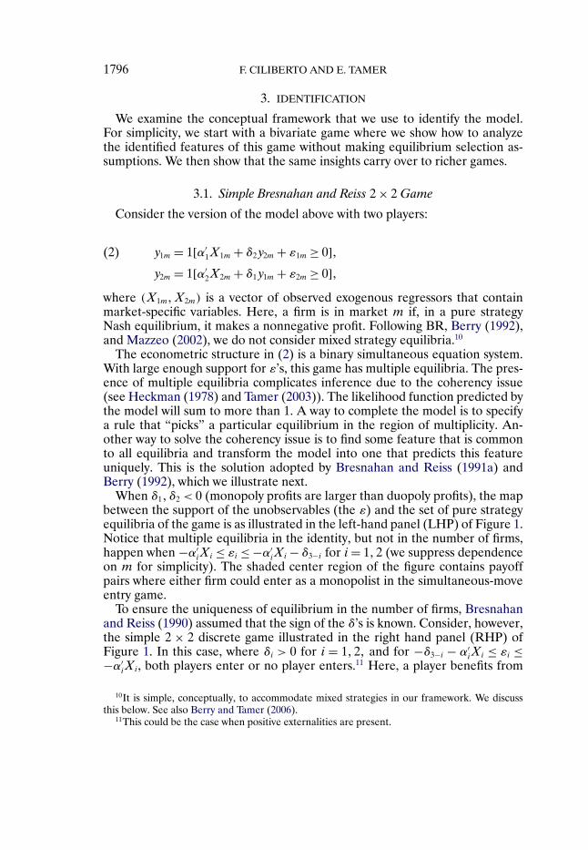
When (1# (2 < 0 (monopoly profits are larger than duopoly profits), the mapbetween the support of the unobservables (the *) and the set of pure strategyequilibria of the game is as illustrated in the left-hand panel (LHP) of Figure 1.Notice that multiple equilibria in the identity, but not in the number of firms,happen when "%#

iXi & *i & "%#iXi " (3"i for i = 1#2 (we suppress dependence

on m for simplicity). The shaded center region of the figure contains payoffpairs where either firm could enter as a monopolist in the simultaneous-moveentry game.

To ensure the uniqueness of equilibrium in the number of firms, Bresnahanand Reiss (1990) assumed that the sign of the (’s is known. Consider, however,the simple 2 ! 2 discrete game illustrated in the right hand panel (RHP) ofFigure 1. In this case, where (i > 0 for i = 1#2# and for "(3"i " %#

iXi & *i &"%#

iXi, both players enter or no player enters.11 Here, a player benefits from

10It is simple, conceptually, to accommodate mixed strategies in our framework. We discussthis below. See also Berry and Tamer (2006).

11This could be the case when positive externalities are present.


FIGURE 1.—Regions for multiple equilibria: LHP, (1# (2 < 0; RHP, (1# (2 > 0.

the other player entering the market. We can again use BR’s approach andestimate the probability of the outcome (1#0), of the outcome (0#1), and ofthe outcome “either (1#1) or (0#0),” but it is clear that we need to know thesign of the (’s. Our methodology does not require knowledge of the signs ofthe (’s.

Finally, with more than two firms, one must assume away any heterogeneityin the effect of observable determinants of profits, including the presence ofa competitor, on the firms’ payoff functions. If one drops these assumptions,different equilibria can exist with different numbers of players, even if the signsof the (’s are known. Heuristically, in three-player games where one player isa large firm and the other two players are small firms, there can be multipleequilibria, where one equilibrium includes the large firm as a monopolist whilethe other has the smaller two firms enter as duopolists (as we will discuss in theempirical section). This happens when one allows differential effect on profitsfrom the entry of a large firm versus a small one ((large $= (small). In contrast,our methodology allows for general forms of heterogeneity in the effect of theobservable determinants of profits.

Main Idea

We illustrate the main idea starting with the case where the (’s are negative.The choice probabilities predicted by the model are

Pr(1#1|X) = Pr(*1 % "%#1X1 " (2;*2 % "%#

2X2 " (1)#(3)

Pr(0#0|X) = Pr(*1 & "%#1X1;*1 & "%#

2X2)#

Pr(1#0|X) = Pr((*1# *2) 'R1(X# "))

+"

Pr((1#0)|*1# *2#X)1[(*1# *2) ' R2("#X)]dF*1#*2#


where

R1("#X) =#(*1# *2) : (*1 % "%#

1X1;*2 & "%#2X2)

( (*1 % "%#1X1 " (2;"%#

2X2 & *2 & "%#2X2 " (1)

$#

R2("#X) =#(*1# *2) : ("%#

1X1 & *1 & "%#1X1 " (2;

" %#2X2 & *2 & "%#

2X2 " (1)$#

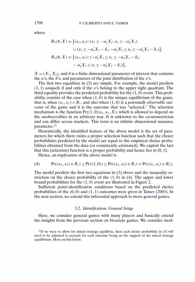
X = (X1#X2), and " is a finite dimensional parameter of interest that containsthe %’s, the (’s, and parameters of the joint distribution of the *’s.

The first two equalities in (3) are simple. For example, the model predicts(1#1) uniquely if and only if the *’s belong to the upper right quadrant. Thethird equality provides the predicted probability for the (1#0) event. This prob-ability consists of the case when (1#0) is the unique equilibrium of the game,that is, when (*1# *2) ' R1, and also when (1#0) is a potentially observable out-come of the game and it is the outcome that was “selected.” The selectionmechanism is the function Pr((1#0)|*1# *2#X), which is allowed to depend onthe unobservables in an arbitrary way. It is unknown to the econometricianand can differ across markets. This term is an infinite dimensional nuisanceparameter.12

Heuristically, the identified feature of the above model is the set of para-meters for which there exists a proper selection function such that the choiceprobabilities predicted by the model are equal to the empirical choice proba-bilities obtained from the data (or consistently estimated). We exploit the factthat this (selection) function is a proper probability and hence lies in [0#1].

Hence, an implication of the above model is

Pr((*1# *2) 'R1)& Pr((1#0))& Pr((*1# *2) ' R1)+ Pr((*1# *2) ' R2)$(4)

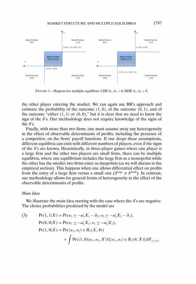
The model predicts the first two equations in (3) above and the inequality re-striction on the choice probability of the (1#0) in (4). The upper and lowerbound probabilities for the (1#0) event are illustrated in Figure 2.

Sufficient point-identification conditions based on the predicted choiceprobabilities of the (0#0) and (1#1) outcomes were given in Tamer (2003). Inthe next section, we extend this inferential approach to more general games.

3.2. Identification: General Setup

Here, we consider general games with many players and basically extendthe insights from the previous section on bivariate games. We consider mod-

12If we were to allow for mixed strategy equilibria, then each choice probability in (3) willneed to be adjusted to account for each outcome being on the support of the mixed strategyequilibrium. More on this below.


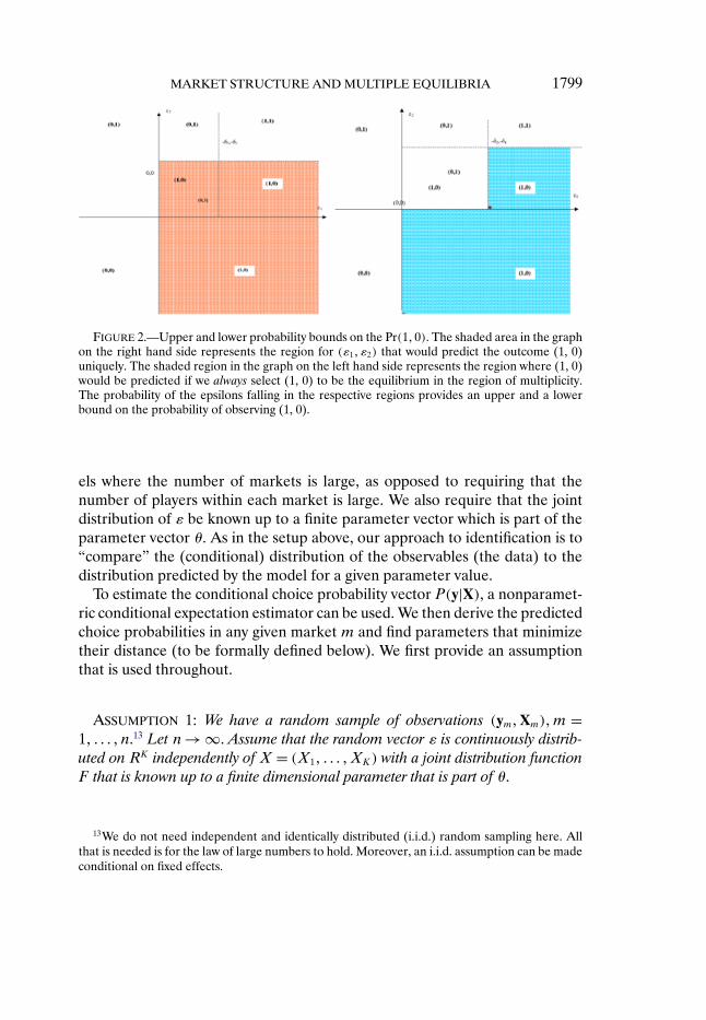
FIGURE 2.—Upper and lower probability bounds on the Pr(1#0). The shaded area in the graphon the right hand side represents the region for (*1# *2) that would predict the outcome (1, 0)uniquely. The shaded region in the graph on the left hand side represents the region where (1, 0)would be predicted if we always select (1, 0) to be the equilibrium in the region of multiplicity.The probability of the epsilons falling in the respective regions provides an upper and a lowerbound on the probability of observing (1, 0).

els where the number of markets is large, as opposed to requiring that thenumber of players within each market is large. We also require that the jointdistribution of * be known up to a finite parameter vector which is part of theparameter vector ". As in the setup above, our approach to identification is to“compare” the (conditional) distribution of the observables (the data) to thedistribution predicted by the model for a given parameter value.

To estimate the conditional choice probability vector P(y|X), a nonparamet-ric conditional expectation estimator can be used. We then derive the predictedchoice probabilities in any given market m and find parameters that minimizetheir distance (to be formally defined below). We first provide an assumptionthat is used throughout.

ASSUMPTION 1: We have a random sample of observations (ym#Xm)#m =1# $ $ $ #n.13 Let n ) *. Assume that the random vector * is continuously distrib-uted on RK independently of X = (X1# $ $ $ #XK) with a joint distribution functionF that is known up to a finite dimensional parameter that is part of ".

13We do not need independent and identically distributed (i.i.d.) random sampling here. Allthat is needed is for the law of large numbers to hold. Moreover, an i.i.d. assumption can be madeconditional on fixed effects.


The predicted choice probability for y # given X is

Pr(y #|X) ="

Pr(y #|*#X)dF

="

R1("#X)

Pr(y #|*#X)dF +"

R2("#X)

Pr(y #|*#X)dF

="

R1("#X)

dF

% &' (unique outcome region

+"

R2("#X)

Pr(y #|*#X)dF

% &' (multiple outcome region

#

where y # = (y #1# $ $ $ # y

#K) is some outcome which is a sequence of 0’s or/and 1’s,

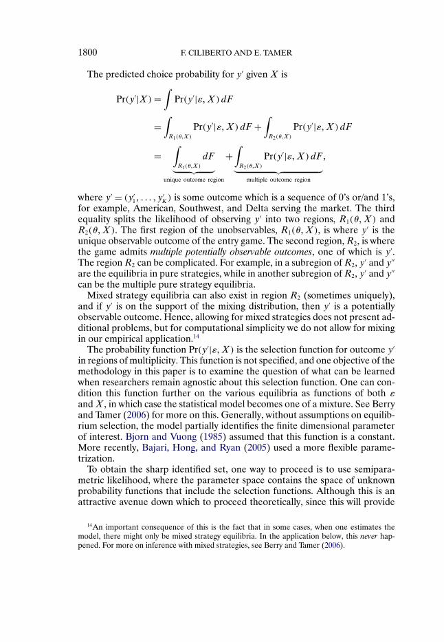
for example, American, Southwest, and Delta serving the market. The thirdequality splits the likelihood of observing y # into two regions, R1("#X) andR2("#X). The first region of the unobservables, R1("#X), is where y # is theunique observable outcome of the entry game. The second region, R2, is wherethe game admits multiple potentially observable outcomes, one of which is y #.The region R2 can be complicated. For example, in a subregion of R2, y # and y ##

are the equilibria in pure strategies, while in another subregion of R2, y # and y ##

can be the multiple pure strategy equilibria.Mixed strategy equilibria can also exist in region R2 (sometimes uniquely),

and if y # is on the support of the mixing distribution, then y # is a potentiallyobservable outcome. Hence, allowing for mixed strategies does not present ad-ditional problems, but for computational simplicity we do not allow for mixingin our empirical application.14

The probability function Pr(y #|*#X) is the selection function for outcome y #

in regions of multiplicity. This function is not specified, and one objective of themethodology in this paper is to examine the question of what can be learnedwhen researchers remain agnostic about this selection function. One can con-dition this function further on the various equilibria as functions of both *and X , in which case the statistical model becomes one of a mixture. See Berryand Tamer (2006) for more on this. Generally, without assumptions on equilib-rium selection, the model partially identifies the finite dimensional parameterof interest. Bjorn and Vuong (1985) assumed that this function is a constant.More recently, Bajari, Hong, and Ryan (2005) used a more flexible parame-trization.

To obtain the sharp identified set, one way to proceed is to use semipara-metric likelihood, where the parameter space contains the space of unknownprobability functions that include the selection functions. Although this is anattractive avenue down which to proceed theoretically, since this will provide

14An important consequence of this is the fact that in some cases, when one estimates themodel, there might only be mixed strategy equilibria. In the application below, this never hap-pened. For more on inference with mixed strategies, see Berry and Tamer (2006).


information on the selection functions, it is difficult to implement practically.15

A practical way to proceed that can be used in many games is to exploit the factthat the selection functions are probabilities and hence bounded between 0and 1, and so an implication of the above model is

"

R1("#X)

dF & Pr(y #|X)&"

R1("#X)

dF +"

R2("#X)

dF$(5)

In vectorized format, these inequalities correspond to the upper and lowerbounds on conditional choice probabilities:

H1(!#X) +

)

*+H1

1(!#X)$$$

H2K1 (!#X)

,

-. &

)

+Pr(y1|X)

$$$Pr(y2K |X)

,

. &

)

*+H1

2(!#X)$$$

H2K2 (!#X)

,

-.(6)

+ H2(!#X)#

where Pr(y|X) (the vector of the form (Pr(0#0)#Pr(0#1)# $ $ $)) is a 2k vector ofconditional choice probabilities. The inequalities are interpreted element byelement.

The H’s are functions of " and of the distribution function F . For example,these functions were derived analytically in (4) for the 2 ! 2 game. The lowerbound function H1 represents the probability that the model predicts a partic-ular market structure as the unique equilibrium.16 H2 contains, in addition, theprobability mass of the region where there are multiple equilibria.

This is a conditional moment inequality model, and the identified feature isthe set of parameter values that obey these restrictions for all X almost every-where and represents the set of economic models that is consistent with theempirical evidence. More formally, we can state the definition:

DEFINITION 1: Let +I be such that

+I = {" '+ s.t. inequalities (6) are satisfied at ", X a.s.}$(7)

We say that +I is the identified set.

In general, the set +I is not a singleton and it is hard to characterizethis set, that is, to find out whether it is finite, convex, etcetera. Next, fol-lowing Tamer (2003), we provide sufficient conditions that guarantee point-identification.

15Another approach to sharp inference in this setup is the recent interesting work ofBeresteanu, Molinari, and Molchanov (2008).

16Notice that there are cross-equation restrictions that can be exploited in the “cube” definedin (5), like the fact that the selection probabilities sum to 1.


3.3. Exclusion Restriction

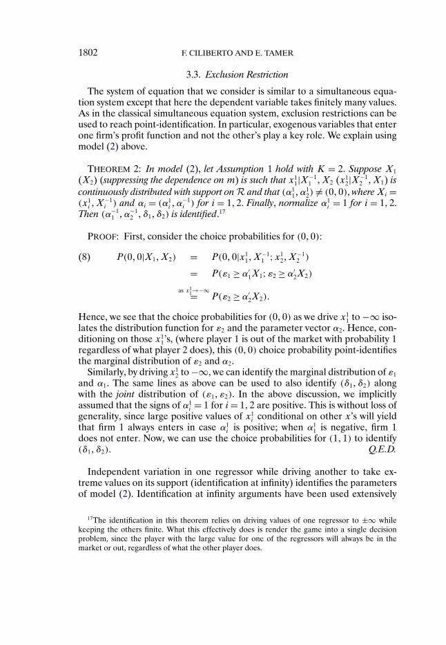
The system of equation that we consider is similar to a simultaneous equa-tion system except that here the dependent variable takes finitely many values.As in the classical simultaneous equation system, exclusion restrictions can beused to reach point-identification. In particular, exogenous variables that enterone firm’s profit function and not the other’s play a key role. We explain usingmodel (2) above.

THEOREM 2: In model (2), let Assumption 1 hold with K = 2. Suppose X1

(X2) (suppressing the dependence on m) is such that x11|X"1

1 #X2 (x12|X"1

2 #X1) iscontinuously distributed with support on R and that (%1

1#%12) $= (0#0), where Xi =

(x1i #X

"1i ) and %i = (%1

i #%"1i ) for i = 1#2. Finally, normalize %1

i = 1 for i = 1#2.Then (%"1

1 #%"12 # (1# (2) is identified.17

PROOF: First, consider the choice probabilities for (0#0):

P(0#0|X1#X2) = P(0#0|x11#X

"11 ;x1

2#X"12 )(8)

= P(*1 % %#1X1;*2 % %#

2X2)

as x11)"*= P(*2 % %#

2X2)$

Hence, we see that the choice probabilities for (0#0) as we drive x11 to "* iso-

lates the distribution function for *2 and the parameter vector %2. Hence, con-ditioning on those x1

1’s, (where player 1 is out of the market with probability 1regardless of what player 2 does), this (0#0) choice probability point-identifiesthe marginal distribution of *2 and %2.

Similarly, by driving x12 to "*, we can identify the marginal distribution of *1

and %1. The same lines as above can be used to also identify ((1# (2) alongwith the joint distribution of (*1# *2). In the above discussion, we implicitlyassumed that the signs of %1

i = 1 for i = 1#2 are positive. This is without loss ofgenerality, since large positive values of x1

i conditional on other x’s will yieldthat firm 1 always enters in case %1

i is positive; when %11 is negative, firm 1

does not enter. Now, we can use the choice probabilities for (1#1) to identify((1# (2). Q.E.D.

Independent variation in one regressor while driving another to take ex-treme values on its support (identification at infinity) identifies the parametersof model (2). Identification at infinity arguments have been used extensively

17The identification in this theorem relies on driving values of one regressor to ±* whilekeeping the others finite. What this effectively does is render the game into a single decisionproblem, since the player with the large value for one of the regressors will always be in themarket or out, regardless of what the other player does.


in econometrics. See, for example, Heckman (1990) and Andrews and Schaf-gans (1998). In more realistic games with many players, variation in excludedexogenous variables (like the airport presence or cost variables we use in theempirical application) help shrink the set +I . The support conditions aboveare sufficient for point identification, and are not essential since our inferencemethods are robust to non-point-identification. However, the exogeneity ofthe regressors and the exclusion restrictions are important restrictions that arediscussed in Section 4.2.

3.4. Estimation

The estimation problem is based on the conditional moment inequalitymodel

H1(!#X)& Pr(y|X) & H2(!#X)$(9)

Our inferential procedures uses the objective function

Q(!)=" /00(P(X)"H1(X#!))"

00 +00(P(X)"H2(X#!))+

001dFx#

where (A)" = [a11[a1 & 0]# $ $ $ #a2k1[a2K & 0]] and similarly for (A)+ for a 2k

vector A, and where - · - is the Euclidian norm. It is easy to see that Q(!) %0 for all " ' + and that Q(!) = 0 if and only if " ' +I , the identified set inDefinition 1.

The object of interest is either the set+I or the (possibly partially identified)true parameter "I '+I . We discuss inference on both "I and+I , but we presentconfidence regions for "I , which is the true but potentially non-point-identifiedparameter that generated the data.18

Statistically, the main difference in whether one considers+I or "I as the pa-rameter of interest is that confidence regions for the former are weakly largerthan for the latter. Evidently, in the case of point-identification, the regionscoincide asymptotically.

Inference in partially identified models is a current area of research ineconometrics, and in this paper we follow the framework of Manski andTamer (2002), Imbens and Manski (2004), and Chernozhukov, Hong, andTamer (2007).19 We discuss first the building of consistent estimators for the

18Earlier versions of the paper contained estimators for sets Cn such that limn)* P(+I . Cn)=%. The current results provide confidence regions for points instead, as the co-editor suggested.The earlier results for the sets, which were not very different, can be obtained from the authorsupon request.

19Other set inference methods that one can use to obtain confidence regions for sets includeAndrews, Berry, and Jia (2003), Beresteanu and Molinari (2008), Romano and Shaikh (2008)Pakes, Porter, Ho, and Ishii (2005), Bugni (2007), and Canay (2007).


identified set, which contains parameters that cannot be rejected as the truth.To estimate +I , we first take a sample analog of Q(·). To do that, we first re-place Pr(y|X) with a consistent estimator Pn(X). Then we define the set 2+I

as

2+I = {" '+ | nQn(") & ,n}#(10)

where ,n ) * and ,n/n ) 0 (take for example ,n = ln(n)) and

Qn(!)= 1n

n!

i=1

/00(Pn(Xi)"H1(Xi# "))"00+

00(Pn(Xi)"H2(Xi# "))+001#(11)

where - ·- is the Euclidian norm. Theorem 3 below shows that the set estimatordefined above is a Hausdorff-consistent estimator of the set +I .

THEOREM 3: Let Assumption 1 hold. Suppose that for the function Qn definedin (11), (i) sup" |Qn(") " Q(")| = Op(1/

/n) and (ii) Qn("I) = Op(1/n) for all

"I '+I . Then we have that with probability (w.p.) approaching 1,

2+I .w$p$1 +I and +I .w$p$12+I as n) *$

PROOF: Following the proof of Theorem 3.1 in CHT, first we show that2+I .w$p$1 +I . This event is equivalent to the event that Q("n) = op(1) for all"n ' 2+I . We have

Q("n) & |Qn("n)"Q("n)| +Qn("n)

= OP(1//n)+Op(,n/n) = op(1)$

On the other hand, we now show that +I .w$p$12+I . This event, again, is equiv-

alent to the event that Qn("I) & ,n/n with probability 1 for all "I ' +I . Fromthe hypothesis of the theorem, we have

Qn("I)= Op(1/n)$

This can be made less than ,n/n with probability approaching 1. Q.E.D.

To conduct inference in the above moment inequalities model, we use themethodology of CHT where the above equality is a canonical example of a mo-ment inequality model. We construct a set Cn such that limn)* P("I ' Cn) % %for a prespecified % ' (0#1) for any "I '+I . In fact, the set Cn that we constructwill not only have the desired coverage property, but will also be consistent inthe sense of Theorem 3. This confidence region is based on the principle of col-lecting all of the parameters that cannot be rejected. The confidence regionswe report are constructed as follows. Let

Cn(c)=3" '+ :n

4Qn(")" min

tQn(t)

5& c

6$(12)


We start with an initial estimate of +I . This set can be, for example, Cn(c0) =Cn(0). Then we will subsample the statistic n(Qn("0) " mint Qn(t)) for "0 'Cn(c0) and obtain the estimate of its %-quantile, c1("0). That is, c1("0) is the %-quantile of {bn(Qbn#j("0)" mint Qbn#j(t))# j = 1# $ $ $ #Bn}. We repeat this for all"0 ' Cn(c0). We take the first updated cutoff c1 to be c1 = sup"0'Cn(c0)

c1("0). Thiswill give us the confidence set Cn(c1). We then redo the above step, replacing c0

with c1, which will get us c2. As the confidence region we can report Cn + Cn(c2)or the generally “smaller”

2+I =3" '+ :n

4Qn(")" min

tQn(t)

5& min(c2# cn("))

6#

where cn(") is the estimated %-quantile of n(Qn(")" mint Qn(t)). In our dataset, we find that there is not much difference between the two, so we re-port Cn(c2). See CHT for more on this and for other ways to build asymp-totically equivalent confidence regions. Also, more on subsampling size andother steps can be found in the online Supplemental Material (Ciliberto andTamer (2009)).

3.5. Simulation

In general games, it is not possible to derive the functions H1 and H2 ana-lytically. Here, we provide a brief description of the simulation procedure thatcan be used to obtain an estimate of these functions for a given X and a givenvalue for the parameter vector ". We first draw R simulations of market andfirm unobservables for each market m. These draws remain fixed during theoptimization stage. We transform the random draw into one with a given co-variance matrix. Then we obtain the “payoffs” for every player i as a function ofother players’ strategies, observables, and parameters. This involves comput-ing a 2k vector of profits for each simulation draw and for every value of ". If!(yj#X# ")% 0 for some j ' {1# $ $ $ #2K}, then yj is an equilibrium of that game.If this equilibrium is unique, then we add 1 to the lower bound probability foroutcome yj and add 1 for the upper bound probability. If the equilibrium isnot unique, then we add a 1 only to the upper bound of each of the multipleequilibria’s upper bound probabilities. For example, the upper bound on theoutcome probability Pr(1#1# $ $ $ #1|X) is

2H2K2 (X# ") = 1

R

R!

j=1

1/!1

7X1# "; y2K

"1# *j1

8% 0# $ $ $ #

!2K7X2K # "; y2K

"2K # *j

2K8% 0

1#


where 1[0] is equal to 1 if the logical condition 0 is true and where R is thenumber of simulations, here we assume that R increases to infinity with samplesize.20

The methods developed by McFadden (1989) and Pakes and Pollard (1989)can be easily used to show that 2Hi(X# ") converges almost surely uniformly in "and X to Hi(X# ") as the number of simulations increases for i = 1#2.

4. MARKET STRUCTURE IN THE U.S. AIRLINE INDUSTRY

Our work contributes to the literature started by Reiss and Spiller (1989)and continued by Berry (1992). Reiss and Spiller (1989) provided evidencethat unobservable firm heterogeneity in different markets is important in de-termining the effect of market power on airline fares. Berry (1992) showedthat firm observable heterogeneity, such as airport presence, plays an impor-tant role in determining airline profitability, providing support to the studiesthat show a strong positive relationship between airport presence and airlinefares.21 Berry also found that profits decline rapidly in the number of enteringfirms, consistent with the findings of Bresnahan and Reiss (1991b).

In this paper, we investigate the role of heterogeneity in the effects that eachfirm’s entry has on the profits of its competitors: we call this their competitiveeffect. Then we use our model to perform a policy exercise on how marketstructures will change, at least in the short run and within our model, in mar-kets out of and into Dallas after the repeal of the Wright Amendment. We startwith a data description.

4.1. Data Description

To construct the data, we follow Berry (1992) and Borenstein (1989). Ourmain data come from the second quarter of the 2001 Airline Origin and Des-tination Survey (DB1B). We discuss the data construction in detail in the Sup-plemental Material. Here, we provide information on the main features of thedata set.

Market Definition

We define a market as the trip between two airports, irrespective of interme-diate transfer points and of the direction of the flight. The data set includes asample of markets between the top 100 metropolitan statistical areas (MSAs),ranked by population size.22 In this sample we also include markets that are

20Since the objective function is nonlinear in the moment condition that contains the simulatedquantities, it is important to drive the number of simulations to infinity; otherwise, there will bea simulation error that does not vanish and can lead to inconsistencies.

21See Borenstein (1989) and Evans and Kessides (1993).22The list of the MSAs is available from the authors.


temporarily not served by any carrier, which are the markets where the num-ber of observed entrants is equal to zero. The selection of these markets isdiscussed in the Supplemental Material. Our data set includes 2742 markets.

Carrier Definition

We focus our analysis on the strategic interaction between American, Delta,United, and Southwest, because one of the objectives of this paper is to de-velop the policy experiment to estimate the impact of repealing the WrightAmendment. To this end, we need to pay particular attention to the nature ofcompetition in markets out of Dallas.

Competition out of Dallas has been under close scrutiny by the Departmentof Justice. In May 1999, the Department of Justice (DOJ) filed an antitrustlawsuit against American Airlines, charging that the major carrier tried to mo-nopolize service to and from its Dallas/Fort Worth (DFW) hub.23 So, usingdata from 2001—the year when American won the case against the DOJ—weinvestigate whether American shows a different strategic behavior than otherlarge firms. Among the other large firms, Delta and United are of particularinterest because they interact intensely with American at its two main hubs:Dallas (Delta) and Chicago O’Hare (United).

In addition to considering American, Delta, United, and Southwest individ-ually, we build two additional categorical variables that indicate the types ofthe remaining firms.24

The categorical variable medium airlines, MAm, is equal to 1 if either Amer-ica West, Continental, Northwest, or USAir is present in market m. Lumpingthese four national carriers into one type makes sense if we believe that theydo not behave in strategically different ways from each other in the marketswe study. To facilitate this assumption, we drop markets where one of the twoendpoints is a hub of the four carriers included in the type medium airlines.25

23In particular, in April 27, 2001, the District Court of Kansas dismissed the DOJ’s case, grant-ing summary judgment to American Airlines. The DOJ’s complaint focused on American’s re-sponses to Vanguard Airlines, Sun Jet, and Western Pacific. In each case, fares dropped dramat-ically and passenger traffic rose when the low cost carriers (LCCs) began operations at DFW.According to the DOJ, American then used a combination of more flights and lower fares un-til the low cost carriers were driven out of the route or drastically curtailed their operations.American then typically reduced service and raised fares back to monopoly levels once the lowcost carriers were forced out of DFW routes. In the lawsuit, the DOJ claimed that American re-sponded aggressively against new entry of low cost carriers in markets out of Dallas/Fort Worth,a charge that was later dismissed.

24In a previous draft of this paper, which is available from the authors’ websites, we showedthat we could also construct vectors of outcomes where an element of the vector is the number ofhow many among Continental, Northwest, America West, and USAir are in the market. This isanalogous to a generalized multivariate version of Berry (1992) and, especially, of Mazzeo (2002).We chose to let MAm and LCCm be categorical variables, since most of the time they take eithera 0 or 1 value.

25See the Supplemental Material for a list of these hubs.


The categorical variable low cost carrier small, LCCm, is equal to 1 if at leastone of the small low cost carriers is present in market m.

4.2. Variable Definitions

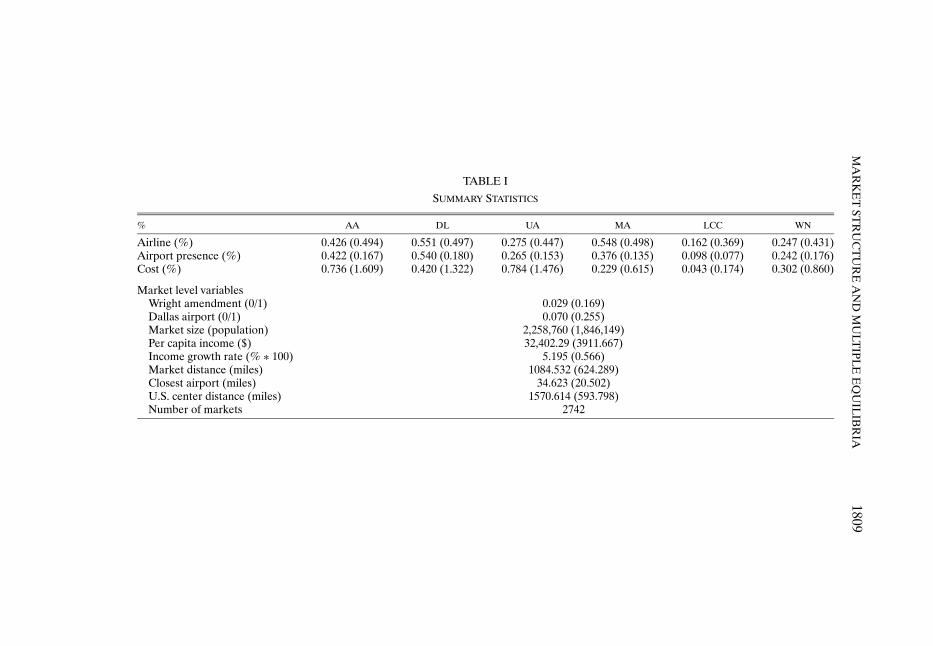
We now introduce the variables used in our empirical analysis. Table Ipresents the summary statistics for these variables.

Airport Presence

Using Berry’s (1992) insight, we construct measures of carrier heterogeneityusing the carrier’s airport presence at the market’s endpoints. First, we computea carrier’s ratio of markets served by an airline out of an airport over the totalnumber of markets served out of an airport by at least one carrier.26 Thenwe define the carrier’s airport presence as the average of the carrier’s airportpresence at the two endpoints. We maintain that the number of markets thatone airline (e.g., Delta) serves out of one airport (e.g., Atlanta) is taken asgiven by the carrier when it decides whether to serve another market.27

Cost

Firm- and market-specific measures of cost are not available. We first com-pute the sum of the geographical distances between a market’s endpoints andthe closest hub of a carrier as a proxy for the cost that a carrier has to faceto serve that market.28 Then we compute the difference between this distanceand the nonstop distance between two airports, and we divide this differenceby the nonstop distance. This measure can be interpreted as the percentage ofthe nonstop distance that the airline must travel in excess of the nonstop dis-tance if the airline uses a connecting instead of a nonstop flight. This is a goodmeasure of the opportunity fixed cost of serving a market, even when a carrierserves that market on a nonstop basis, because it measures the cost of the bestalternative to nonstop service, which is a connecting flight through the closesthub. It is associated with the fixed cost of providing airline service because it isa function of the total capacity of a plane, but does not depend on the numberof passengers transported on a particular flight. We call this variable cost.

26See the discussion in the Supplemental Material for more on this.27The entry decision in each market is interpreted as a “marginal” decision, which takes the

network structure of the airline as given. This marginal approach to the study of the airline mar-kets is also used in the literature that studies the relationship between market concentration andpricing. For example, Borenstein (1989) and Evans and Kessides (1993) did not include pricesin other markets out of Atlanta (e.g., ATL-ORD) to explain fares in the market ATL-AUS. Thereason for this marginal approach is that modeling the design of a network is too complicated.

28Data on the distances between airports, which are also used to construct the variable closeairport are from the data set Aviation Support Tables: Master Coordinate, available from the Na-tional Transportation Library. See the Supplemental Material for the list of hubs.

MA

RK

ET

STR

UC

TU

RE

AN

DM

ULT

IPLE

EQ

UIL

IBR

IA1809

TABLE ISUMMARY STATISTICS

% AA DL UA MA LCC WN

Airline (%) 0.426 (0.494) 0.551 (0.497) 0.275 (0.447) 0.548 (0.498) 0.162 (0.369) 0.247 (0.431)Airport presence (%) 0.422 (0.167) 0.540 (0.180) 0.265 (0.153) 0.376 (0.135) 0.098 (0.077) 0.242 (0.176)Cost (%) 0.736 (1.609) 0.420 (1.322) 0.784 (1.476) 0.229 (0.615) 0.043 (0.174) 0.302 (0.860)

Market level variablesWright amendment (0/1) 0.029 (0.169)Dallas airport (0/1) 0.070 (0.255)Market size (population) 2,258,760 (1,846,149)Per capita income ($) 32,402.29 (3911.667)Income growth rate (% 0 100) 5.195 (0.566)Market distance (miles) 1084.532 (624.289)Closest airport (miles) 34.623 (20.502)U.S. center distance (miles) 1570.614 (593.798)Number of markets 2742


The Wright Amendment

The Wright Amendment was passed in 1979 to stimulate the growth of theDallas/Fort Worth airport. To achieve this objective, Congress restricted air-line service out of Dallas Love, the other major airport in the Dallas area. Inparticular, the Wright Amendment permitted air carrier service between LoveField and airports only in Texas, Louisiana, Arkansas, Oklahoma, New Mexico,Alabama, Kansas, and Mississippi, provided that the air carrier did not permitthrough service or ticketing and did not offer for sale transportation outsideof these states.29 In October 2006, a bill was enacted that determined the fullrepeal of the Wright Amendment in 2014. Between 2006 and 2014, nonstopflights outside the Wright zone would still be banned, connecting flights out-side the Wright zone would be allowed immediately, and only domestic flightswould be allowed out of Dallas Love.

We construct a binary variable, Wright, equal to 1 if entry into the marketis regulated by the Wright Amendment, and equal to 0 otherwise. Wright isequal to 1 for the markets between Dallas Love and any airport except theones located in Texas, Louisiana, Arkansas, Oklahoma, New Mexico, Alabama,Kansas, and Mississippi.

We also construct another categorical variable, called Dallas market, whichis equal to 1 if the market is between either of the two Dallas airports andany other airport in the data set. This variable controls for the presence of aDallas fixed effect. More details on the Wright Amendment are given in theSupplemental Material.

Control Variables

We use six control variables. Three of these are demographic variables.30

The geometric mean of the city populations at the market endpoints measuresthe market size. The average per capita incomes (per capita income) and theaverage rates of income growth (income growth rate) of the cities at the marketendpoints measure the strength of the economies at the market endpoints.The other three variables are geographic. The nonstop distance between theendpoints is the measure of market distance. The distance from each airport tothe closest alternative airport controls for the possibility that passengers can flyfrom different airports to the same destination (close airport).31 Finally, we use

29The Shelby Amendment, passed in 1997, dropped the original restriction on flights betweenDallas Love and airports in Alabama, Kansas, and Mississippi. In 2005, an amendment was passedthat exempted Missouri from the Wright restrictions.

30Data are from the Regional Economic Accounts of the Bureau of Economic Analysis, down-load in February 2005.

31For example, Chicago Midway is the closest alternative airport to Chicago O’Hare. Noticethat for each market, we have two of these distances, since we have two endpoints. Our variableis equal to the minimum of these two distances. In previous versions of the paper, we addressedthe concern that many large cities have more than one airport. For example, it is possible to fly


the sum of the distances from the market endpoints to the geographical centerof the United States (U.S. center distance). This variable is intended to controlfor the fact that, just for purely geographical reasons, cities in the middle of theUnited State have a larger set of close cities than cities on the coasts or citiesat the borders with Mexico and Canada.32

Market Size Does Not Explain Market Structure

To motivate the analysis that follows, we have classified markets by marketsize of the connected cities. The relevant issue is whether market size alonedetermines market structure (Bresnahan and Reiss (1990)). Table II providessome evidence that the variation in the number of firms across markets cannotbe explained by market size alone.

Identification in Practice

We assume that the unobservables are not correlated with our exogenousvariables. This is part of the content of Assumption 1. Notice that this assump-tion would be clearly violated if we were to use variables that the firm can

TABLE IIDISTRIBUTION OF THE NUMBER OF CARRIERS BY MARKET SIZEa

Number ofFirms Large Medium Small Total

0 7$07 7$31 7$73 7$291 41$51 22$86 20$91 30$632 29$03 24$30 22$14 25$933 12$23 19$67 16$34 15$724 8$07 15$14 14$59 11$935 1$66 9$58 16$17 7$486 0$42 1$13 2$11 1$02Number 1202 971 569 2742

aCross-tabulation of the percentage of firms serving a market by the market size,which is here measured by the geometric mean of the populations at the marketendpoints.

from San Francisco to Washington on nine different routes. In a previous version of the paper,we allowed the firms’ unobservables to be spatially correlated across markets between the sametwo cities. In the estimation, whenever a market was included in the subsample that we drew toconstruct the parameter bounds, we also included any other market between the same two cities.This is similar to adjusting the moment conditions to allow for spatial correlation. In our context,it was easy to adjust for it since we knew which of the observations were correlated, that is, onesthat had airports in close proximity.

32The location of the mean center of population is from the Geography Division at the U.S.Bureau of the Census. Based on the 1990 census results, it was located in Crawford County,Missouri.


choose, such as prices or quantities. However, we are considering a reducedform profit function, where all of the control variables (e.g., population, dis-tance) are maintained to be exogenous.33

The main difficulty of estimating model (1) is given by the presence of thecompetitors’ entry decisions, since we consider a simultaneous move entrygame. Theorem 2 in Section 3.3 shows that an exclusion restriction helps topoint identify "I . Here, an exclusion restriction consists of a variable that en-ters firm i’s profit but not firm j’s. If this variable has wide support (e.g., a largedegree of variation), then this reduces the size of the identified set.

Berry (1992) assumed that the variable airport presence of one carrier is ex-cluded from the profit equations of its competitors. Then airport presence is amarket–carrier-specific variable that shifts the individual profit functions with-out changing the competitors’ profit functions. We refer to this model as thefixed competitive effect specification (that is, )i

j = 0 ,i# j). For example, the air-port presence of American is excluded from the profit function of Delta. Inthe version fixed competitive effects we have two exclusion restrictions. Both theairport presence (used by Berry) and the cost of the competitors are excludedfrom the profit function.

The second version of model (1) that we estimate is called variable compet-itive effects. This version includes the market presence of one airline in theprofit function of all airlines. As mentioned in the Introduction, the theoreti-cal underpinnings for these variable competitive effects are in Hendricks, Pic-cione, and Tan (1997). In this version, variable competitive effects, only the costvariable shifts the individual profit functions without changing the competitors’profit functions, while airport presence is included in the profit functions of allfirms.

Generally, the economic rationale for excluding the competitors’ cost but in-cluding their airport presence in a firm’s profit function is the following. The air-port presence variable is a measure of product differentiation. Thus, the airportpresence of each firm is likely to enter the demand side of the profit function ofall firms.34 In contrast, a variable that affects the fixed cost of one firm directlyenters the (reduced form) profit function of only that firm.35

We maintain that this variable does not enter the profit function of the com-petitors directly.

33The presence of market-, airport-, and airline-specific random effects controls for unob-served heterogeneity in the data.

34Berry (1990) used airport presence as a measure of product differentation in a discrete choicemodel of demand for airline travel.

35Notice that variables affecting the variable costs would not work as instruments because theywould enter into the reduced form profit functions. The excluded variables must be determinantsof the fixed cost.


Reporting of Estimates

In our results, we report superset confidence regions that cover the truth, "I ,with a prespecified probability. This parameter might be partially identified,and hence our confidence intervals are robust to non-point-identification.Since generically these models are not point identified, and since the true pa-rameter, along with all parameters in the identified set, minimize a nonlinearobjective function, it is not possible to provide estimates of the bounds on thetrue parameter.36 So our reported confidence regions have the coverage prop-erty and can also be used as consistent estimators for the bounds of the partiallyidentified parameter "I . So in each table, we report the cube that contains theconfidence region that is defined as the set that contains the parameters thatcannot be rejected as the truth with at least 95% probability.37

5. EMPIRICAL RESULTS

Before discussing our results, we specify in detail the error structure of ourempirical model and discuss the first stage estimation.

First, we include firm-specific unobserved heterogeneity, uim.38 Then we addmarket-specific unobserved heterogeneity, um. Finally, we add airport-specificunobserved heterogeneity uo

m and udm, where uo

m is an error that is commonacross all markets whose origin is o and ud

m is an error that is common across allmarkets whose origin is d$39 uim, um, uo

m, and udm are independent and normally

distributed, except where explicitly mentioned. Recall that *im is the sum of allfour errors.

With regard to the first stage estimation of the empirical probabilities, wefirst discretize the variables and then use a nonparametric frequency estimator.We discuss the way we discretize the variables in the Supplemental Material.The nonparametric frequency estimator consists of counting the fraction ofmarkets with a given realization of the exogenous variables where we observea given market structure.40

36The reason is that it is not possible to solve for the upper and lower endpoints of the bounds,especially in a structural model where the objective function is almost always mechanically mini-mized at a unique point.

37Not every parameter in the cube belongs to the confidence region. This region can containholes, but here we report the smallest connected “cube” that contains the confidence region.

38In one specification (third column of Table IV in Section 5.2), we estimate the covariancematrix of the unobserved variables (reported in Table VI).

39Recall that our markets are defined irrespective of the direction of the flight. Thus, the useof the terms “origin” and “destination” means either one of the market endpoints.

40An alternative to discretization and nonparametric estimation is to add a distributional as-sumption in the first stage. In previous versions of the paper, we estimated the empirical proba-bilities using a multinomial logit. This discretization is necessary since inference procedures witha nonparametric first step with continuous regressors have not been developed.


5.1. Fixed Competitive Effects

This section provides the estimation results for model (1) when we restrict)i

j = )j = 0 ,i# j$ Essentially, this is the same specification as the one used byBresnahan and Reiss (1990) and Berry (1992), and therefore it provides theideal framework with which to compare our methodology. This first version isalso useful for investigating the case where the competitive effect of one air-line is allowed to vary by the identity of its competitors. For example we allowDelta’s effect on American to be different than Delta’s effect on Southwest.In this case, the number of parameters to be estimated gets large very quickly.Thus, this specification allows for a more flexible degree of heterogeneity thatis computationally very difficult to have without restricting )i

j = 0 ,i# j$

Berry Specification

The second column of Table III presents the estimation results for a variantof the model estimated by Berry (1992). Here we assume &i = &, %i = %, and(ij = ( ,i# j. Most importantly, this implies that the effects of firms on eachother, measured by (, are identical.

In the second column of Table III, the reported confidence interval is the“usual” 95% confidence interval since the coefficients are point identified. Themain limitation of this model is that the effects of firms on each other areidentical, which ensures that in each market there is a unique equilibrium inthe number of firms.

The parameter competitive fixed effect captures the effect of the number offirms on the probability of observing another firm entering a market. We esti-mate the effect of an additional firm to be ["14$151#"10$581]. The entry of afirm lowers the probability that we see its competitors in the market.

As the number of markets that an airline serves at an airport increases,the probability that the firm enters into the market increases as well. Thisis seen from the positive effect of airport presence, which is [3$052#5$087].As expected, the higher is the value of the variable cost, the lower is theprobability that the firm serves that market (["0$714#0$024]). A higher in-come growth rate increases the probability of entry ([0$370#1$003]), as domarket size ([0$972#2$247]), U.S. center distance ([1$452#3$330]), market dis-tance ([4$356#7$046]), per capita income ([0$568#2$623]), and close airport([4$022#9$831]). The Wright Amendment has a negative impact on entry, asits coefficient is estimated to be ["20$526#"8$612].

Next, we present values of the distance function at the parameter valueswhere this function is minimized. In the first column, the distance functiontakes the value 1756$2. This function can be interpreted as a measure of “fit”among different specifications that use the same exogenous variables.

Berry’s (1992) (symmetry) assumptions ensure that the equilibrium is uniquein the number of firms, though there might be multiple equilibria in the identityof firms. To examine the existence of multiple equilibria in the identity of firms,

MA

RK

ET

STR

UC

TU

RE

AN

DM

ULT

IPLE

EQ

UIL

IBR

IA1815

TABLE IIIEMPIRICAL RESULTSa

Heterogeneous Heterogeneous Firm-to-FirmBerry (1992) Interaction Control Interaction

Competitive fixed effect ["14.151, "10.581]AA ["10.914, "8.822] ["9.510, "8.460]DL ["10.037, "8.631] ["9.138, "8.279]UA ["10.101, "4.938] ["9.951, "5.285]MA ["11.489, "9.414] ["9.539, "8.713]LCC ["19.623, "14.578] ["19.385, "13.833]WN ["12.912, "10.969] ["10.751, "9.29]LAR on LAR

LAR: AA, DL, UA, MA ["9.086, "8.389]LAR on LCC ["20.929, "14.321]LAR on WN ["10.294, "9.025]LCC on LAR ["22.842, "9.547]WN on LAR ["9.093, "7.887]LCC on WN ["13.738, "7.848]WN on LCC ["15.950, "11.608]

Airport presence [3.052, 5.087] [11.262, 14.296] [10.925, 12.541] [9.215, 10.436]Cost ["0.714, 0.024] ["1.197, "0.333] ["1.036, "0.373] ["1.060, "0.508]Wright ["20.526, "8.612] ["14.738, "12.556] ["12.211, "10.503] ["12.092, "10.602]Dallas ["6.890, "1.087] ["1.186, 0.421] ["1.014, 0.324] ["0.975, 0.224]Market size [0.972, 2.247] [0.532, 1.245] [0.372, 0.960] [0.044, 0.310]

WN [0.358, 0.958]LCC [0.215, 1.509]

(Continues)

1816F.C

ILIB

ER

TO

AN

DE

.TAM

ER

TABLE III—Continued

Heterogeneous Heterogeneous Firm-to-FirmBerry (1992) Interaction Control Interaction

Market distance [4.356, 7.046] [0.106, 1.002] [0.062, 0.627] ["0.057, 0.486]WN ["2.441, "1.121]LCC ["0.714, 1.858]

Close airport [4.022, 9.831] ["0.769, 2.070] ["0.289, 1.363] ["1.399,"0.196]WN [1.751, 3.897]LCC [0.392, 5.351]

U.S. center distance [1.452, 3.330] ["0.932, "0.062] ["0.275, 0.356] ["0.606, 0.242]WN ["0.357, 0.860]LCC ["1.022, 0.673]

Per capita income [0.568, 2.623] ["0.080, 1.010] [0.286, 0.829] [0.272, 1.073]Income growth rate [0.370, 1.003] [0.078, 0.360] [0.086, 0.331] [0.094, 0.342]Constant ["13.840, "7.796] ["1.362, 2.431] ["1.067, "0.191] [0.381, 2.712]

MA ["0.016, 0.852]LCC ["2.967, "0.352]WN ["0.448, 1.073]

Function value 1756.2 1644.1 1627 1658.3Multiple in identity 0.837 0.951 0.943 0.969Multiple in number 0 0.523 0.532 0.536Correctly predicted 0.328 0.326 0.325 0.308

a These set estimates contain the set of parameters that cannot be rejected at the 95% confidencet level. See Chernozhukov, Hong, and Tamer (2007) and the SupplementalMaterial for more details on constructing these confidence regions.


we simulate results and find that in 83.7% of the markets there exist multipleequilibria in the identity of firms.

Finally, we report the percentage of outcomes that are correctly predictedby our model. Clearly, in each market we only observe one outcome in thedata. The model, however, predicts several equilibria in that market. If one ofthem is the outcome observed in the data, then we conclude that our modelpredicted the outcome correctly. We find that our model predicts 32.8% of theoutcomes in the data. This is also a measure of fit that can be used to comparemodels.

Heterogeneous Competitive Fixed Effects

The third column allows for firms to have different competitive effects ontheir competitors. We relax the assumption (ij = ( ,i# j. Here we only assume(ij = (j ,i# j. For example, the effect of American’s presence on Southwest’sand Delta’s entry decisions is given by (AA, while the effect of Southwest’s pres-ence on the decision of the other airlines is given by (WN.

All the (’s are estimated to be negative, which is in line with the intuitionthat profits decline when other firms enter a market. There is quite a bit ofheterogeneity in the effects that firms have on each other. The row denoted AAreports the estimates for the effect of American on the decision of the otherairlines to enter into the market. We estimate the effect of American on theother airlines to be ["10$914#"8$822]. Instead, the entry decision of low costcarriers (LCC) has a slightly stronger effect on other airlines. The estimate ofthis effect is ["19$623#"14$578].

The coefficient estimates for the control variables are quite different inthe second and third columns. This suggests that assuming symmetry in-troduces some bias in the estimates of the exogenous variables. For exam-ple, in the second column we estimate the effect of market distance to be[4$356#7$046], while in the third column the effect is [0$106#1$002]. The es-timates for the constant are also different: ["13$840#"7$796] in the secondcolumn and ["1$362#2$431] in the third column.

The differences in the competitive effects are large enough to lead to mul-tiple equilibria in the number of firms in 52.3% percent of the markets. Thus,even the simplest form of heterogeneity introduces the problem of multipleequilibria in a fundamental way. Next, we show that multiple equilibria canalso be present when we allow for other types of heterogeneity in the empiricalmodel.

Control Variables With Heterogeneous Fixed Effects

The fourth column allows the control variables to have different effects onthe profits of firms. In practice we drop the assumption %i = % ,i. This is inter-esting because relaxing this assumption leads to multiple equilibria, even if thecompetitive effects are the same across firms.


We estimate market size to have a similar positive effect on the probabilitythat all firms enter into a market (the estimated sets overlap). On the contrary,we find that market distance increases the probability of entry of large nationalcarriers, but it has a negative effect on the entry decision of Southwest. This isconsistent with anecdotal evidence that Southwest serves shorter markets thanthe larger national carriers.

Firm-to-Firm Specific Competitive Effects

We now allow Delta’s effect (Delta’s effect is coded as the effect of a (LAR)large type firm) on American (whose effect is also coded as the effect of a typeLAR firm) to be different than Delta’s effect on Southwest (WN). Here, thecompetitive effects of American (AA), Delta (DL), United (UA), and the typeMA are coded as the effect of a type LAR firm. Therefore, (LAR

LAR measuresthe competitive effect of the entry of a large carrier, for example, American,on another large carrier, for example, Delta. (WN

LAR measures the competitiveeffect of Southwest on one of the four LAR firms. The other parameters aredefined similarly. We find that the competitive effect of large firms on otherlarge firms (LAR on LAR or (LAR

LAR) is ["9$086#"8$389], which is smaller thanthe competitive effect of large firms on low cost firms (LAR on LCC). Thecompetitive effects are not symmetric, in the sense that (LCC

LAR is larger than (LARLCC .

Finally, the competitive effects of Southwest and large firms on each other aresymmetric. Overall, these results suggest that the competitive effects are firm-to-firm specific. In later specifications, we do not allow for the competitiveeffects to vary in this very general way to reduce the number of parameters tobe estimated. However, we find that allowing for variable competitive effectsand for a flexible variance–covariance structure leads to results that are equallyrich in terms of firm-to-firm effects.

5.2. Variable Competitive Effects

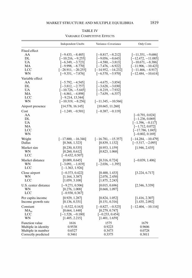
In this section, we study models where the competitive effect of a firm on theother carriers’ profits from serving that market varies with its airport presence.Here, the main focus is on the estimation of )j .41

Variable Competitive Effects With Independent Unobservables

The second column of Table IV reports the estimation results when the er-rors are assumed to be i.i.d. Most importantly, the coefficients )j , which mea-sure the variable competitive effects, are all negative, as we would expect. Thisimplies that the larger is the airport presence of an airline, the less likely is theentry of its competitors in markets where the airline is present.

41We restrict )ij =)j for computational reasons.


TABLE IVVARIABLE COMPETITIVE EFFECTS

Independent Unobs Variance–Covariance Only Costs

Fixed effectAA ["9.433, "8.485] ["8.817, "8.212] ["11.351, "9.686]DL ["10.216, "9.255] ["9.056, "8.643] ["12.472, "11.085]UA ["6.349, "3.723] ["4.580, "3.813] ["10.671, "8.386]MA ["9.998, "8.770] ["7.476, "6.922] ["11.906, "10.423]LCC ["28.911, "20.255] ["14.952, "14.232] ["11.466, "8.917]WN ["9.351, "7.876] ["6.570, "5.970] ["12.484, "10.614]

Variable effectAA ["5.792, "4.545] ["4.675, "3.854]DL ["3.812, "2.757] ["3.628, "3.030]UA ["10.726, "5.645] ["8.219, "7.932]MA ["6.861, "4.898] ["7.639, "6.557]LCC ["9.214, 13.344]WN ["10.319, "8.256] ["11.345, "10.566]

Airport presence [14.578, 16.145] [10.665, 11.260]Cost ["1.249, "0.501] ["0.387, "0.119]

AA ["0.791, 0.024]DL ["1.236, 0.069]UA ["1.396, "0.117]MA ["1.712, 0.072]LCC ["17.786, 1.045]WN ["0.802, 0.169]

Wright ["17.800, "16.346] ["16.781, "15.357] ["14.284, "10.479]Dallas [0.368, 1.323] [0.839, 1.132] ["5.517, "2.095]Market size [0.230, 0.535] [0.953, 1.159] [1.946, 2.435]

WN [0.260, 0.612] [0.823, 1.068]LCC ["0.432, 0.507]

Market distance [0.009, 0.645] [0.316, 0.724] ["0.039, 1.406]WN ["3.091, "1.819] ["2.036, "1.395]LCC ["1.363, 1.926]

Close airport ["0.373, 0.422] [0.400, 1.433] [3.224, 6.717]WN [1.164, 3.387] [2.078, 2.450]LCC [1.059, 3.108] [1.875, 2.243]

U.S. center distance ["9.271, 0.506] [0.015, 0.696] [2.346, 3.339]WN [0.276, 1.008] [0.668, 1.097]LCC ["0.930, 0.367]

Per capita income [0.929, 1.287] [0.824, 1.052] [1.416, 2.307]Income growth rate [0.136, 0.331] [0.151, 0.316] [1.435, 2.092]Constant ["0.522, 0.163] ["0.827, "0.523] ["12.404, "10.116]

MAm [0.664, 1.448] [0.279, 0.747]LCC ["1.528, "0.180] ["0.233, 0.454]WN [1.405, 2.215] [1.401, 1.659]

Function value 1616 1575 1679Multiple in identity 0.9538 0.9223 0.9606Multiple in number 0.6527 0.3473 0.0728Correctly predicted 0.3461 0.3375 0.3011


We compare these results to those presented in the fourth column of Ta-ble III. To facilitate the comparison it is worth mentioning that in Table III,the competitive effect of one firm (for example, American) on the others iscaptured by a constant term, for example, (AA. In Table IV, the same com-petitive effect is captured by a linear function of American’s airport presence,(AA +)AAZAA#m. Our findings suggests that both the fixed and variable effectsare negative. For example, we find (AA equal to ["9$433#"8$485] and )AA

equal to ["5$792#"4$545]. Thus, a firm’s entry lowers the probability of ob-serving other firms in the market. Moreover, the larger is the airport presenceof the firm, the smaller is the probability of a competitor’s entry. This is con-sistent with the idea that entry is less likely when the market is being served byanother firm that is particularly attractive, because of the positive effect on thedemand of airport presence.

Variable Competitive Effects With Correlated Unobservables

In the third column, we relax the i.i.d. assumption on the unobservables andestimate the variance–covariance matrix.42 Notice that the results are quitesimilar in the second and third columns. For this reason, here we provide a dis-cussion on the economic magnitude (that is, the marginal effects) of the para-meters estimated in the third column.

Table V presents the marginal effects of the variables. The results are or-ganized in three panels. The top and middle panels show the marginal effectsassociated with a unit discrete change.43 The bottom panel shows the effectthat the entry of a carrier, for example, American, has on the probability thatwe observe one of its competitors in the market.

Before presenting our results, we clarify up front an important point. Nor-mally, the marginal effects are a measure of how changes in the variables of themodel affect the probability of observing the discrete event that is being stud-ied. Here, there are six discrete events that our model must predict, as many asthe carriers that can enter into a market, and there are eight market structuresin which we can observe any given carrier. For example, we can observe Amer-ican as a monopoly, as a duopoly with Delta or United, and so on. If therewere no multiple equilibria, this would not create any difficulty: We could sim-ply sum over the probability of all the market structures where American is inthe market and that would give us the total probability of observing Americanin the market. However, we do have multiple equilibria, and we only observe

42This correlation structure of the unobservable errors allows the unobservable profits of thefirms to be correlated. For example, in markets where large firms face high fuel costs, small firmsalso face high fuel costs. Another possibility is that there are unobservable characteristics of amarket that we are unable to observe, and that affect large firms and Southwest differently, sothat when American enters, Southwest does not and vice versa.

43Recall that we have discretized our data.


TABLE VMARGINAL EFFECTSa

AA DL UA MA LCC WN No Firms

Market sizePositive 0$1188 0$1136 0$0571 0$1188 0$0849 0$1118 "0$0033Negative "0$0494 "0$0720 "0$0001 "0$0442 "0$1483 "0$0300 "0$0033

Market distancePositive 0$0177 0$0165 0$0106 0$0177 0$0099 0$0000 0$0006Negative "0$0354 "0$0377 "0$0110 "0$0360 "0$0128 "0$0377 0$0006

Close airportPositive 0$1178 0$1122 0$0312 0$1048 0$0662 0$1178 "0$0033Negative "0$0375 "0$0518 "0$0004 "0$0318 -0$0911 "0$0175 "0$0033

Change incomePositive 0$0283 0$0265 0$0149 0$0283 0$0171 0$0277 "0$0007Negative "0$0140 "0$0193 "0$0001 "0$0120 "0$0339 "0$0086 "0$0007

Per capita incomePositive 0$0576 0$0546 0$0291 0$0576 0$0364 0$0573 "0$0015Negative "0$0270 "0$0377 "0$0002 "0$0237 "0$0699 "0$0160 "0$0015

U.S. center distancePositive 0$0177 0$0181 0$0052 0$0171 0$0038 0$0181 "0$0004Negative "0$0044 "0$0055 "0$0001 "0$0033 "0$0076 "0$0011 "0$0004

Airport presence 0$0673 0$0498 0$1888 0$0734 0$0599 0$1040Cost "0$0102 "0$0068 "0$0117 "0$0120 "0$0054 "0$0125

AA · · · "0$3606 "0$2556 "0$4108 "0$0704 "0$2143DL "0$3336 · · · "0$2658 "0$3908 "0$0335 "0$2126UA "0$2486 "0$2630 · · · "0$2696 "0$0675 "0$2015MA "0$3877 "0$3941 "0$2717 · · · "0$0989 "0$2766LCC "0$0998 "0$1579 "0$0721 "0$1415 · · · "0$0411WN "0$2256 "0$2356 "0$2030 "0$2868 "0$0242 · · ·

aThe numbers that we report are marginal effects. They are appropriately selected percentage changes in theoriginal probability of a particular outcome. In the top and middle panels we report the largest change in the averageupper bounds of the probabilities of observing a given carrier in any possible market structure.

lower and upper bounds on the probabilities of each market structure. Sum-ming over the upper bounds of the probabilities of the market structures whereAmerican is in the market is not the appropriate solution, because the maxi-mum probability of observing one market structure, for example, an Americanmonopoly, necessarily excludes seeing another market structure, for example,a duopoly with American and Delta, with its maximum probability.

There is one important exception to the point just made. The probability ofobserving the market structure with no firms is uniquely identified because thecompetitive effects are negative. Thus, in our discussion we will pay particularattention to this outcome, where no firm enters into a market.


In the top and middle panels, we report the largest positive and negativechange in the average upper bounds of the probabilities of observing a givencarrier in any possible market structure. We report both the positive and neg-ative changes because an increase in market size, for example, increases theprofits of all firms. Thus, all firms individually are more likely to enter. How-ever, here we are looking at the simultaneous decision of all firms. Conse-quently, we may see that some market structures become more likely to beobserved at the expense of other market structures. The dominant effect forone particular firm might end up being negative. We identify the dominanteffects in italics.

In practice, we increase one variable at a time and we compute the averageby an economically meaningful amount and we compute the average upperbounds by taking the means of the upper bounds for one market structureacross markets. Then we compute the average upper bounds by taking themeans of the upper bounds for one market structure across markets at theobserved values. Finally, we take the differences of all of the upper bounds forall 64 market structures, and report the largest positive and negative changesamong them.

In the top panel, an increase in market size of 1 million people is associatedwith a maximum effect of an increase of 11$88% in the probability of observingAmerican Airlines and a maximum decrease of "4$94% of not observing it.This means that there is one market structure where American is present thatis 11$88% percent more likely to be observed and there is one other marketstructure where American is present that is 4$94% less likely to be observed.We interpret this combination of results as evidence that an increase in mar-ket size is associated with an overall increase in the likelihood of observingAmerican in a market.

If the nonstop distance increases by 250 miles, then the overall likelihoodof observing American in a market decreases by 3$54%. If the distance to theclosest alternative airport increases by more than 50 miles, then the probabilityof observing American increases by 11$78%. If income grows 1% faster, thenthe probability of observing American serving the market increases by 2$83%.If the per capita income increases by 5,000 dollars, then the maximum prob-ability of observing a market structure where American is serving the mar-ket increases by 5$76 percent. Finally, if the distance from the US geographi-cal center increases of 250 miles, then the maximum probability of observingAmerican increases by 1$77 percent. The interpretation of the results for theother firms is analogous.

The middle panel reports the effect of an increase in the variables measuringheterogeneity on the probability of observing an airline, or no airlines (“NoFirms”), in the market. Generally, the effects are much larger in this middlepanel than in the top panel, suggesting that observable heterogeneity is a keydeterminant of entry. If American’s airport presence increases by 15%, thenthe probability of observing American increases by 6$73%. Finally, an increase


TABLE VIVARIANCE–COVARIANCE MATRIX

AA DL UA MA LCC WN

AA 1 [0.043, 0.761] ["0.110, 0.442] [0.103, 0.626] ["0.217, 0.752] [0.055, 0.355]DL [5.052, 6.895] ["0.200, 0.190] [0.629, 0.949] ["0.128, 0.656] [0.218, 0.834]UA [2.048, 3.340] ["0.173, 0.309] ["0.213, 0.652] [0.192, 0.797]MA [2.396, 5.558] ["0.094, 0.313] [0.093, 0.862]LCC [2.026, 6.705] [0.093, 0.764]WN [2.063, 2.331]

of 50% in the cost associated with serving a market lowers the probability ofobserving American by approximately 1%.44

The numbers in the bottom panel of Table V are derived in a slightly differ-ent fashion from those ones in the top and middle panels. They also requireadditional discussion. Let us say that we want to quantify the effect of Ameri-can’s entry on the probability of observing one of its competitors. If there wereunique equilibria, then the answer would be straightforward. We could set theparameters that measure the competitive effects of American equal to zeroand then recompute the new equilibria. Then we would just have to computethe change in the probabilities of observing the other firms in each market andtake the averages across all markets. With multiple equilibria, the analysis ofthe marginal effects has to take into account that we estimate lower and upperbounds for the probability of observing any market structure in each market.

We find that Delta’s entry can decrease the probability of observing Ameri-can in the market by as much as 33$36%. The effect of Delta’s entry varies a lotby the identity of the opponent, as we observe that it is just "3$35% for lowcost carriers.

Next, we discuss the estimation results for the variance–covariance matrix.Recall that the unobservables are made up of four components. One of them isa firm-specific component. We estimate the covariances of these firm-specificcomponents. In addition, we estimate the variance of the sum of the four com-ponents.

We find that the variances of all firms are larger than one. For example,the variance for Delta is [5$052#6$895]. This suggests that the unobservableheterogeneity for these firms is larger than for American.

The estimated correlations are quite interesting. In general, it is hard toidentify correlation coefficients among unobservables in multivariate discretechoice models, and here is no exception since the confidence regions are wide.A few points are worth making. For example, the unobservables of Southwest

44We do not report the negative effect, since for the variable airport presence, the increase inthe maximum probability of observing a firm in one particular market structure is always largerin absolute value than the maximum decrease of observing that firm in another market structure.


and low cost carriers are positively correlated, suggesting that it is more likelythat both of them would be in a market, ceteris paribus.

Only Costs

The fourth column of Table IV estimates the model without the variablesthat measure airport presence. In practice, we set &i = & = 0, in addition to(ij = (j and )i

j = )j = 0 ,i# j. We present this specification so as to addressthe concern that airport presence could be endogenous if airlines choose theirnetwork, instead of choosing only whether to enter into a particular market fora given exogenous network. This concern is particularly reasonable when weperform our policy simulation. The results should be compared with those thethird in column of Table III. With the exception of Southwest, the fixed com-petitive effects are all similar. This is reassuring because it suggests that thevariation in the costs is enough to identify the competitive effects. This specifi-cation fits the data less than the specification in the third column of Table III.

6. POLICY EXPERIMENT: THE REPEAL OF THE WRIGHT AMENDMENT

We develop a policy experiment to examine how our model predicts themarket structures change in markets out of Dallas Love after the repeal ofthe Wright Amendment. To this end, it is crucial to study the individual firms’strategic responses to the repeal of the amendment. In practice, we first takeall 93 markets out of Dallas Love and simulate the predicted outcomes with theWright Amendment still in place. We then repeal the law (we set the variableWright equal to zero) and recompute the new predicted outcomes. Followingthe same approach as when we computed the marginal effects, we report themaximum change in the average upper bounds of the probabilities of observinga given carrier in any possible market structure before and after the repeal ofthe Wright Amendment. Our estimates provide a within model prediction ofthe effect of the repeal that should be interpreted in the short term.

In Table VII, we present the policy simulations when we use three differentspecifications.

The second column of Table VII reports the policy results when we use thespecification in the third column of Table IV. This is an interesting specifica-tion because it accounts for correlation in the unobservables. We report theresults when we use the value of the parameters at which the objective func-tion is minimized. This is the number in the middle. Then we report the lowestand largest numbers for the policy results that we derive when we use all theparameters in the estimated set.

The first result of interest is in the first row, which reports the probabilityof observing markets not served by any carrier. We find that the percentage ofmarkets that would not be served would drop by 63$84% after the repeal of theWright Amendment, suggesting that its repeal would increase the number ofmarkets served out of Dallas Love. Of those new markets, as many as 47$44%


TABLE VIIPREDICTED PROBABILITIES FOR POLICY ANALYSIS: MARKETS OUT OF DALLAS LOVE

Airline Variance–Covariance Independent Obs Only Costs

No firms ["0.6514, "0.6384, "0.6215] ["0.7362, "0.6862, "0.6741] ["0.6281, "0.6162, "0.5713]AA [0.4448, 0.4634, 0.4711] [0.2067, 0.3013, 0.3280] [0.3129, 0.3782, 0.4095]DL [[0.4768, 0.4988, 0.5056] 0.2733, 0.3774, 0.4033] [0.3843, 0.4315, 0.4499]UA [0.1377, 0.1467, 0.1519] [0.1061, 0.1218, 0.2095] [0.2537, 0.3315, 0.3753]MA [0.4768, 0.4988, 0.5056] [0.2733, 0.3774, 0.4033] [0.3656, 0.4143, 0.4342]LCC [0.3590, 0.3848, 0.4156] [0.8369, 0.8453, 0.8700] [0.2839, 0.3771, 0.3933]WN [0.4480, 0.4744, 0.4847] [0.2482, 0.2697, 0.3367] [0.3726, 0.4228, 0.4431]

could be served by Southwest. American and Delta, which have strong airportpresences at Dallas/Fort Worth would serve a percentage of these markets,that is, at most 46$34 and 49$88% respectively.

These marked changes in market structures suggest that one reason why theWright Amendment was not repealed until 2006 was to protect American mo-nopolies in markets out of Dallas/Fort Worth. Repealing the Wright Amend-ment would lead to a remarkable increase in service in new markets out ofDallas Love and thus would reduce the incentive for American to prevent en-try of new competitors in markets out of Dallas/Fort Worth. As we said, theseare dramatic increases and they do raise some concern that our methodologymight overestimate the effects of the repeal of the Wright Amendment.

First, we tried to get some anecdotal information on how Southwest plansto react to the repeal of the Wright Amendment. We checked Southwest’s webpage and found out that since the partial repeal of the Wright Amendmentin October 2006, Southwest has started offering one-stop, same plane or con-necting service itineraries to and from Dallas Love field to 43 cities beyondthe Wright Amendment area. This pattern of entry into new markets confirmsthat the repeal of the Wright Amendment is bound to have dramatic effects onairline service out of the Dallas Love airport.

As a second check, we compared our results with those that we would deriveusing the coefficient estimates in the second column of Table IV. The mainresult, concerning the change in the number of markets that are not served, isalmost identical. The other results, with the exception of that for the low costcarriers, are very similar.

Finally, we checked our predictions using a specification where the airportpresence variables are not included. The policy change might be so major thatfirms change their network structure when the Wright Amendment is repealed.The fourth column of Table VII reports the policy results when we use thespecification presented in the fourth column of Table IV. This last specificationshows results that are almost identical to those in the third column of Table VII.


7. CONCLUSIONS

This paper is a first step in the development of methods that study inferencein entry models without making equilibrium selection assumptions. To that ex-tent, these methods are used to study the effect of multiple equilibria on learn-ing about parameters of interest. However, the methodology used in this pa-per has important limitations. The model imposes distributional assumptionson the joint distribution of the unobservables and on the shape of the variableprofit function. Though it is conceptually possible to study the identificationproblem in our model without making strong parametric assumptions, it is notclear at this point that those results are practically attractive since they willinvolve a semiparametric model with possibly partially identified parameters.

Moreover, the empirical analysis of the paper looks at the airline industryand network from a long-run perspective where its network is taken as exoge-nous in the short run. To relax this assumption, one needs to use a more compli-cated model that accounts for the dynamics of entry and of adjustment to oneairline’s network in response to entry by a competitor. This is something we donot pursue here. Hence, the results, especially the policy experiments, need tobe interpreted as the response in the short run and within our model. On theother hand, the econometric model allows for flexible correlation among firmunobservables and for spatial correlation among market unobservables. In ad-dition, it is possible to test whether a certain selection mechanism is consistentwith the data and the model by verifying whether estimates obtained undera given mechanism lie in our sets. To do that, one needs to deal with modelmisspecification, a topic that we leave also for future research.

REFERENCES

ANDREWS, D. W. K., AND M. SCHAFGANS (1998): “Semiparametric Estimation of the Interceptof a Sample Selection Model,” Review of Economic Studies, 65, 487–517. [1803]

ANDREWS, D. W. K., AND G. SOARES (2009): “Inference for Parameters Defined by MomentInequalities Using Generalize Moment Selection,” Econometrica (forthcoming). [1792]

ANDREWS, D., S. BERRY, AND P. JIA (2003): “On Placing Bounds on Parameters of Entry Gamesin the Presence of Multiple Equilibria,” Working Paper, Yale University. [1794,1803]

ARADILLAS-LOPEZ, A. (2005): “Semiparametric Estimation of a Simultaneous Game With In-complete Information,” Working Paper, Princeton University. [1793]

BAJARI, P., H. HONG, AND S. RYAN (2005): “Identification and Estimation of Discrete Games ofComplete Information,” Working Paper, Stanford University. [1793,1800]

BERESTEANU, A., AND F. MOLINARI (2008): “Asymptotic Properties for a Class of Partially Iden-tified Models,” Econometrica, 76, 763–814. [1792,1803]

BERESTEANU, A., F. MOLINARI, AND I. MOLCHANOV (2008): “Sharp Identification Regions inGames,” Working Paper, Cornell University. [1801]

BERRY, S. (1990): “Airport Presence as Product Differentiation,” American Economic Review,Papers and Proceedings, 80, 394–399. [1812]

(1992): “Estimation of a Model of Entry in the Airline Industry,” Econometrica, 60,889–917. [1791,1792,1794,1796,1806-1808,1812,1814-1816]

BERRY, S., AND E. TAMER (2006): “Identification in Models of Oligopoly Entry,” in Advancesin Economics and Econometrics. Ninth World Congress of the Econometric Society, Vol. 2, ed.

http://www.e-publications.org/srv/ecta/linkserver/setprefs?rfe_id=urn:sici%2F0012-9682%28200911%2977%3A6%3C1791%3AMSAMEI%3E2.0.CO%3B2-Z

http://www.e-publications.org/srv/ecta/linkserver/openurl?rft_dat=bib:1/andrewsschafgans&rfe_id=urn:sici%2F0012-9682%28200911%2977%3A6%3C1791%3AMSAMEI%3E2.0.CO%3B2-Z

http://www.e-publications.org/srv/ecta/linkserver/openurl?rft_dat=bib:2/andrewssoares&rfe_id=urn:sici%2F0012-9682%28200911%2977%3A6%3C1791%3AMSAMEI%3E2.0.CO%3B2-Z

http://www.e-publications.org/srv/ecta/linkserver/openurl?rft_dat=bib:6/molinariset&rfe_id=urn:sici%2F0012-9682%28200911%2977%3A6%3C1791%3AMSAMEI%3E2.0.CO%3B2-Z

http://www.e-publications.org/srv/ecta/linkserver/openurl?rft_dat=bib:8/berry90&rfe_id=urn:sici%2F0012-9682%28200911%2977%3A6%3C1791%3AMSAMEI%3E2.0.CO%3B2-Z


http://www.e-publications.org/srv/ecta/linkserver/openurl?rft_dat=bib:1/andrewsschafgans&rfe_id=urn:sici%2F0012-9682%28200911%2977%3A6%3C1791%3AMSAMEI%3E2.0.CO%3B2-Z

http://www.e-publications.org/srv/ecta/linkserver/openurl?rft_dat=bib:2/andrewssoares&rfe_id=urn:sici%2F0012-9682%28200911%2977%3A6%3C1791%3AMSAMEI%3E2.0.CO%3B2-Z

http://www.e-publications.org/srv/ecta/linkserver/openurl?rft_dat=bib:6/molinariset&rfe_id=urn:sici%2F0012-9682%28200911%2977%3A6%3C1791%3AMSAMEI%3E2.0.CO%3B2-Z





by R. Blundell, W. Newey, and T. Persson. Cambridge: Cambridge University Press, 46–85.[1794,1796,1800]

BJORN, P., AND Q. VUONG (1985): “Simultaneous Equations Models for Dummy EndogenousVariables: A Game Theoretic Formulation With an Application to Labor Force Participation,”Working Paper 537, Caltech. [1793,1800]

BLUNDELL, R., M. BROWNING, AND I. CRAWFORD (2003): “Nonparametric Engel Curves andRevealed Preference,” Econometrica, 71, 205–240. [1794]

BLUNDELL, R., A. GOSLING, H. ICHIMURA, AND C. MEGHIR (2007): “Changes in the Distribu-tion of Male and Female Wages Accounting for Employment Composition,” Econometrica, 75,323–363. [1794]

BORENSTEIN, S. (1989): “Hubs and High Fares: Dominance and Market Power in the US AirlineIndustry,” RAND Journal of Economics, 20, 344–365. [1806,1808]

BORZEKOWSKI, R., AND A. COHEN (2004): “Estimating Strategic Complementarities in CreditUnions’ Outsourcing Decisions,” Working Paper, Fed. [1795]

BRESNAHAN, T. (1989): “Empirical Studies of Industries With Market Power,” in Handbook ofIndustrial Organization, Vol. 2, ed. by R. Schmalensee and R. Willig. North-Holland. [1795]

BRESNAHAN, T., AND P. REISS (1990): “Entry in Monopoly Markets,” Review of Economic Studies,57, 531–553. [1791,1796,1811,1814]

(1991a): “Empirical Models of Discrete Games,” Journal of Econometrics, 48, 57–81.[1796]

(1991b): “Entry and Competition in Concentrated Markets,” Journal of Political Econ-omy, 99, 977–1009. [1806]

BUGNI, F. (2007): “Bootstrap Inference in Partially Identified Models,” Working Paper, North-western University. [1792,1803]

CANAY, I. (2007): “EL Inference for Partially Identified Models: Large Deviations Optimalityand Bootstrap Validity,” Working Paper, Northwestern. [1792,1803]

CHERNOZHUKOV, V., H. HONG, AND E. TAMER (2007): “Estimation and Confidence Regions forParameter Sets in Econometric Models,” Econometrica, 75, 1243–1284. [1792,1803,1816]

CILIBERTO, F., AND E. TAMER (2009): “Supplements to ‘Market Structure and MultipleEquilibria in Airline Markets’,” Econometrica Supplemental Material, 77, http://www.econometricsociety.org/ecta/Supmat/5368_simulations.pdf; http://www.econometricsociety.org/ecta/Supmat/5368_data and programs. zip. [1805]

EVANS, W., AND I. KESSIDES (1993): “Localized Market Power in the U.S. Airline Industry,”Review of Economics and Statistics, 75, 66–75. [1806,1808]

FRISCH, R. (1934): Statistical Confluence Analysis. Oslo: University Institute of Economics. [1794]HAILE, P., AND E. TAMER (2003): “Inference With an Incomplete Model of English Auctions,”

Journal of Political Economy, 111, 1–51. [1794]HECKMAN, J. (1978): “Dummy Endogenous Variables in a Simultaneous Equation System,”

Econometrica, 46, 931–960. [1796](1990): “Varieties of Selection Bias,” The American Economic Review, 80, 313–318.

[1803]HECKMAN, J. J., AND E. J. VYTLACIL (1999): “Local Instrumental Variables and Latent Variable

Models for Identifying and Bounding Treatement Effects,” Proceedings of the National Academyof Science: Economic Sciences, 96, 4730–4734. [1794]

HECKMAN, J., R. LALONDE, AND J. SMITH (1999): “The Economics and Econometrics of ActiveMarket Programs,” in Handbook of Labor Economics, ed. by O. Ashenfelter and D. Card.Amsterdam: North Holland, Chap. 31. [1794]

HENDRICKS, K., M. PICCIONE, AND G. TAN (1997): “Entry and Exit in Hub-Spoke Networks,”RAND Journal of Economics, 28, 291–303. [1793,1812]

HONORÉ, B., AND A. LLERAS-MUNEY (2006): “Bounds in Competing Risks Models and the Waron Cancer,” Econometrica, 74, 1675–1698. [1794]

IMBENS, G., AND C. F. MANSKI (2004): “Confidence Intervals for Partially Identified Parameters,”Econometrica, 72, 1845–1857. [1794,1803]

http://www.e-publications.org/srv/ecta/linkserver/openurl?rft_dat=bib:12/blundellbrowningcrawford&rfe_id=urn:sici%2F0012-9682%28200911%2977%3A6%3C1791%3AMSAMEI%3E2.0.CO%3B2-Z

http://www.e-publications.org/srv/ecta/linkserver/openurl?rft_dat=bib:13/blundellichicosta&rfe_id=urn:sici%2F0012-9682%28200911%2977%3A6%3C1791%3AMSAMEI%3E2.0.CO%3B2-Z

http://www.e-publications.org/srv/ecta/linkserver/openurl?rft_dat=bib:14/borenstein2&rfe_id=urn:sici%2F0012-9682%28200911%2977%3A6%3C1791%3AMSAMEI%3E2.0.CO%3B2-Z

http://www.e-publications.org/srv/ecta/linkserver/openurl?rft_dat=bib:17/bresreissrestud&rfe_id=urn:sici%2F0012-9682%28200911%2977%3A6%3C1791%3AMSAMEI%3E2.0.CO%3B2-Z

http://www.e-publications.org/srv/ecta/linkserver/openurl?rft_dat=bib:18/bresnahanreissdiscrete&rfe_id=urn:sici%2F0012-9682%28200911%2977%3A6%3C1791%3AMSAMEI%3E2.0.CO%3B2-Z

http://www.e-publications.org/srv/ecta/linkserver/openurl?rft_dat=bib:19/1991b&rfe_id=urn:sici%2F0012-9682%28200911%2977%3A6%3C1791%3AMSAMEI%3E2.0.CO%3B2-Z

http://www.e-publications.org/srv/ecta/linkserver/openurl?rft_dat=bib:22/cht&rfe_id=urn:sici%2F0012-9682%28200911%2977%3A6%3C1791%3AMSAMEI%3E2.0.CO%3B2-Z

http://www.econometricsociety.org/ecta/Supmat/5368_simulations.pdf

http://www.econometricsociety.org/ecta/Supmat/5368_data%20and%20programs.zip

http://www.e-publications.org/srv/ecta/linkserver/openurl?rft_dat=bib:24/evanskessides&rfe_id=urn:sici%2F0012-9682%28200911%2977%3A6%3C1791%3AMSAMEI%3E2.0.CO%3B2-Z

http://www.e-publications.org/srv/ecta/linkserver/openurl?rft_dat=bib:26/hailetamer&rfe_id=urn:sici%2F0012-9682%28200911%2977%3A6%3C1791%3AMSAMEI%3E2.0.CO%3B2-Z

http://www.e-publications.org/srv/ecta/linkserver/openurl?rft_dat=bib:27/Heckman78&rfe_id=urn:sici%2F0012-9682%28200911%2977%3A6%3C1791%3AMSAMEI%3E2.0.CO%3B2-Z

http://www.e-publications.org/srv/ecta/linkserver/openurl?rft_dat=bib:28/heckman1990&rfe_id=urn:sici%2F0012-9682%28200911%2977%3A6%3C1791%3AMSAMEI%3E2.0.CO%3B2-Z

http://www.e-publications.org/srv/ecta/linkserver/openurl?rft_dat=bib:29/heckmanmte&rfe_id=urn:sici%2F0012-9682%28200911%2977%3A6%3C1791%3AMSAMEI%3E2.0.CO%3B2-Z

http://www.e-publications.org/srv/ecta/linkserver/openurl?rft_dat=bib:31/hendricksetal&rfe_id=urn:sici%2F0012-9682%28200911%2977%3A6%3C1791%3AMSAMEI%3E2.0.CO%3B2-Z

http://www.e-publications.org/srv/ecta/linkserver/openurl?rft_dat=bib:32/boadriana&rfe_id=urn:sici%2F0012-9682%28200911%2977%3A6%3C1791%3AMSAMEI%3E2.0.CO%3B2-Z

http://www.e-publications.org/srv/ecta/linkserver/openurl?rft_dat=bib:33/manskiimbens&rfe_id=urn:sici%2F0012-9682%28200911%2977%3A6%3C1791%3AMSAMEI%3E2.0.CO%3B2-Z

http://www.e-publications.org/srv/ecta/linkserver/openurl?rft_dat=bib:12/blundellbrowningcrawford&rfe_id=urn:sici%2F0012-9682%28200911%2977%3A6%3C1791%3AMSAMEI%3E2.0.CO%3B2-Z



http://www.e-publications.org/srv/ecta/linkserver/openurl?rft_dat=bib:14/borenstein2&rfe_id=urn:sici%2F0012-9682%28200911%2977%3A6%3C1791%3AMSAMEI%3E2.0.CO%3B2-Z

http://www.e-publications.org/srv/ecta/linkserver/openurl?rft_dat=bib:17/bresreissrestud&rfe_id=urn:sici%2F0012-9682%28200911%2977%3A6%3C1791%3AMSAMEI%3E2.0.CO%3B2-Z

http://www.e-publications.org/srv/ecta/linkserver/openurl?rft_dat=bib:18/bresnahanreissdiscrete&rfe_id=urn:sici%2F0012-9682%28200911%2977%3A6%3C1791%3AMSAMEI%3E2.0.CO%3B2-Z



http://www.e-publications.org/srv/ecta/linkserver/openurl?rft_dat=bib:22/cht&rfe_id=urn:sici%2F0012-9682%28200911%2977%3A6%3C1791%3AMSAMEI%3E2.0.CO%3B2-Z

http://www.econometricsociety.org/ecta/Supmat/5368_simulations.pdf

http://www.econometricsociety.org/ecta/Supmat/5368_data%20and%20programs.zip

http://www.e-publications.org/srv/ecta/linkserver/openurl?rft_dat=bib:24/evanskessides&rfe_id=urn:sici%2F0012-9682%28200911%2977%3A6%3C1791%3AMSAMEI%3E2.0.CO%3B2-Z

http://www.e-publications.org/srv/ecta/linkserver/openurl?rft_dat=bib:26/hailetamer&rfe_id=urn:sici%2F0012-9682%28200911%2977%3A6%3C1791%3AMSAMEI%3E2.0.CO%3B2-Z

http://www.e-publications.org/srv/ecta/linkserver/openurl?rft_dat=bib:27/Heckman78&rfe_id=urn:sici%2F0012-9682%28200911%2977%3A6%3C1791%3AMSAMEI%3E2.0.CO%3B2-Z

http://www.e-publications.org/srv/ecta/linkserver/openurl?rft_dat=bib:28/heckman1990&rfe_id=urn:sici%2F0012-9682%28200911%2977%3A6%3C1791%3AMSAMEI%3E2.0.CO%3B2-Z



http://www.e-publications.org/srv/ecta/linkserver/openurl?rft_dat=bib:31/hendricksetal&rfe_id=urn:sici%2F0012-9682%28200911%2977%3A6%3C1791%3AMSAMEI%3E2.0.CO%3B2-Z

http://www.e-publications.org/srv/ecta/linkserver/openurl?rft_dat=bib:32/boadriana&rfe_id=urn:sici%2F0012-9682%28200911%2977%3A6%3C1791%3AMSAMEI%3E2.0.CO%3B2-Z

http://www.e-publications.org/srv/ecta/linkserver/openurl?rft_dat=bib:33/manskiimbens&rfe_id=urn:sici%2F0012-9682%28200911%2977%3A6%3C1791%3AMSAMEI%3E2.0.CO%3B2-Z


MANSKI, C. F. (1990): “Nonparametric Bounds on Treatment Effects,” The American EconomicReview, 80, 319–323. [1794]

(1994): “The Selection Problem,” in Advances in Econometrics: Sixth World Congress.Econometric Society Monographs, Vol. 2, ed. by C. Sims. Cambridge: Cambridge UniversityPress, 143–170. [1794]

(2007): Identification for Prediction and Decision. Cambridge, MA: Harvard UniversityPress. [1794]

MANSKI, C. F., AND E. TAMER (2002): “Inference on Regressions With Interval Data on a Re-gressor or Outcome,” Econometrica, 70, 519–547. [1794,1803]

MARSCHAK, J., AND W. H. ANDREWS (1944): “Random Simultaneous Equations and the Theoryof Production,” Econometrica, 12, 143–203. [1794]

MAZZEO, M. (2002): “Product Choice and Oligopoly Market Structure,” RAND Journal of Eco-nomics, 33, 1–22. [1795,1796,1807]

MCFADDEN, D. (1989): “A Method of Simulated Moments for Estimation of Discrete ResponseModels Without Numerical Integration,” Econometrica, 57, 995–1026. [1806]

PAKES, A., AND D. POLLARD (1989): “Simulation and the Asymptotics of Optimization Estima-tors,” Econometrica, 57, 1027–1057. [1806]

PAKES, A., J. PORTER, K. HO, AND J. ISHII (2005): “Moment Inequalities and Their Applica-tions,” Working Paper, Harvard University. [1794,1803]

PETERSON, A. V. (1976): “Bounds for a Joint Distribution Function With Fixed SubdistributionFunctions: Applications to Competing Risks,” Proceedings of the National Academy of Sciencesof the United States of America, 73, 11–13. [1794]

REISS, P., AND P. SPILLER (1989): “Competition and Entry in Small Airline Markets,” Journal ofLaw and Economics, 32, S179–S202. [1806]

ROMANO, J., AND A. SHAIKH (2008): “Inference for the Identified Set in Partially IdentifiedEconometric Models,” Journal of Statistical Planning and Inference, 138, 2786–2807. [1792,1803]

SEIM, K. (2002): “An Empirical Model of Firm Entry With Endogenous Product-Type Choices,”Working Paper, Stanford Business School. [1793]

SUTTON, J. (1991): Sunk Costs and Market Structure: Price Competition, Advertising, and the Evo-lution of Concentration. Cambridge, MA: MIT Press. [1792]

(2000): Marshall’s Tendencies: What Can Economists Know? Cambridge, MA: MIT Press.[1792]

SWEETING, A. (2004): “Coordination Games, Multiple Equilibria, and the Timing of Radio Com-mercials,” Working Paper, Duke University. [1793]

TAMER, E. (2003): “Incomplete Bivariate Discrete Response Model With Multiple Equilibria,”Review of Economic Studies, 70, 147–167. [1792,1796,1798,1801]

Dept. of Economics, University of Virginia, Monroe Hall, Charlottesville, VA22903, U.S.A.; [email protected]

andDept. of Economics, Northwestern University, 2001 Sheridan Road, Evanston,

IL 60208, U.S.A.; [email protected].

Manuscript received August, 2004; final revision received February, 2009.

http://www.e-publications.org/srv/ecta/linkserver/openurl?rft_dat=bib:34/manskiaer&rfe_id=urn:sici%2F0012-9682%28200911%2977%3A6%3C1791%3AMSAMEI%3E2.0.CO%3B2-Z

http://www.e-publications.org/srv/ecta/linkserver/openurl?rft_dat=bib:35/manskiworldcongress&rfe_id=urn:sici%2F0012-9682%28200911%2977%3A6%3C1791%3AMSAMEI%3E2.0.CO%3B2-Z

http://www.e-publications.org/srv/ecta/linkserver/openurl?rft_dat=bib:37/tamermanski&rfe_id=urn:sici%2F0012-9682%28200911%2977%3A6%3C1791%3AMSAMEI%3E2.0.CO%3B2-Z

http://www.e-publications.org/srv/ecta/linkserver/openurl?rft_dat=bib:38/marschakandrews&rfe_id=urn:sici%2F0012-9682%28200911%2977%3A6%3C1791%3AMSAMEI%3E2.0.CO%3B2-Z

http://www.e-publications.org/srv/ecta/linkserver/openurl?rft_dat=bib:39/mazzeo&rfe_id=urn:sici%2F0012-9682%28200911%2977%3A6%3C1791%3AMSAMEI%3E2.0.CO%3B2-Z

http://www.e-publications.org/srv/ecta/linkserver/openurl?rft_dat=bib:40/mcfadden89&rfe_id=urn:sici%2F0012-9682%28200911%2977%3A6%3C1791%3AMSAMEI%3E2.0.CO%3B2-Z

http://www.e-publications.org/srv/ecta/linkserver/openurl?rft_dat=bib:41/pakespollard89&rfe_id=urn:sici%2F0012-9682%28200911%2977%3A6%3C1791%3AMSAMEI%3E2.0.CO%3B2-Z

http://www.e-publications.org/srv/ecta/linkserver/openurl?rft_dat=bib:43/petersonbounds&rfe_id=urn:sici%2F0012-9682%28200911%2977%3A6%3C1791%3AMSAMEI%3E2.0.CO%3B2-Z

http://www.e-publications.org/srv/ecta/linkserver/openurl?rft_dat=bib:44/reissspiller&rfe_id=urn:sici%2F0012-9682%28200911%2977%3A6%3C1791%3AMSAMEI%3E2.0.CO%3B2-Z

http://www.e-publications.org/srv/ecta/linkserver/openurl?rft_dat=bib:45/romanoshaikh&rfe_id=urn:sici%2F0012-9682%28200911%2977%3A6%3C1791%3AMSAMEI%3E2.0.CO%3B2-Z

http://www.e-publications.org/srv/ecta/linkserver/openurl?rft_dat=bib:50/tamer2&rfe_id=urn:sici%2F0012-9682%28200911%2977%3A6%3C1791%3AMSAMEI%3E2.0.CO%3B2-Z

mailto:[email protected]

mailto:[email protected]

http://www.e-publications.org/srv/ecta/linkserver/openurl?rft_dat=bib:34/manskiaer&rfe_id=urn:sici%2F0012-9682%28200911%2977%3A6%3C1791%3AMSAMEI%3E2.0.CO%3B2-Z




http://www.e-publications.org/srv/ecta/linkserver/openurl?rft_dat=bib:37/tamermanski&rfe_id=urn:sici%2F0012-9682%28200911%2977%3A6%3C1791%3AMSAMEI%3E2.0.CO%3B2-Z

http://www.e-publications.org/srv/ecta/linkserver/openurl?rft_dat=bib:38/marschakandrews&rfe_id=urn:sici%2F0012-9682%28200911%2977%3A6%3C1791%3AMSAMEI%3E2.0.CO%3B2-Z

http://www.e-publications.org/srv/ecta/linkserver/openurl?rft_dat=bib:39/mazzeo&rfe_id=urn:sici%2F0012-9682%28200911%2977%3A6%3C1791%3AMSAMEI%3E2.0.CO%3B2-Z

http://www.e-publications.org/srv/ecta/linkserver/openurl?rft_dat=bib:40/mcfadden89&rfe_id=urn:sici%2F0012-9682%28200911%2977%3A6%3C1791%3AMSAMEI%3E2.0.CO%3B2-Z

http://www.e-publications.org/srv/ecta/linkserver/openurl?rft_dat=bib:41/pakespollard89&rfe_id=urn:sici%2F0012-9682%28200911%2977%3A6%3C1791%3AMSAMEI%3E2.0.CO%3B2-Z



http://www.e-publications.org/srv/ecta/linkserver/openurl?rft_dat=bib:44/reissspiller&rfe_id=urn:sici%2F0012-9682%28200911%2977%3A6%3C1791%3AMSAMEI%3E2.0.CO%3B2-Z

http://www.e-publications.org/srv/ecta/linkserver/openurl?rft_dat=bib:45/romanoshaikh&rfe_id=urn:sici%2F0012-9682%28200911%2977%3A6%3C1791%3AMSAMEI%3E2.0.CO%3B2-Z

http://www.e-publications.org/srv/ecta/linkserver/openurl?rft_dat=bib:50/tamer2&rfe_id=urn:sici%2F0012-9682%28200911%2977%3A6%3C1791%3AMSAMEI%3E2.0.CO%3B2-Z

Documents

Market Structure and Multiple Equilibria in Airline Marketsmshum/gradio/papers/ecta5368.pdf · market structure and multiple equilibria in airline markets ... market structure and