Managing Groundwater Levels in an Agricultural Area with

e Hulaage canalster levelsgreen coverelds. Thed

r a periodwithin the

Peat.

Managing Groundwater Levels in an Agricultural Area withPeat Soils

Nir Naveh, M.ASCE,1 and Uri Shamir, F.ASCE2

Abstract: The Hula Decision Support System~HDSS! is designed to aid Hula site operators in managing groundwater levels in thLake region of Israel. Groundwater levels are managed by controlling water levels by using adjustable dams in a grid of drainand by the timing and intensity of irrigation. Water levels in the canals are controlled by a set of hydraulic structures. Groundwaare to be maintained within a specified range to minimize decomposition and subsidence of the peat soils, ensure year-roundof the area, and avoid saturation conditions in the crop root zone, thereby allowing farmers to continue cultivation of their fimanagement module for the HDSS performs optimization with the following two objectives:~1! minimize deviation from the specifiegroundwater target level, and~2! minimize supply of water from the Jordan River to the Hula drainage canals~water quantity is limited!.The second objective is achieved indirectly in the HDSS by determining the dam settings and irrigation quantity and timing oveof eight weeks and then solving again whenever conditions change. The results are checked by simulation using MODFLOWGMS modeling package. The procedure is demonstrated and analyzed.

DOI: 10.1061/~ASCE!0733-9496~2004!130:3~243!

CE Database subject headings: Decision support systems; Ground water; Agriculture; Water levels; Optimization; Irrigation;

sel. Aalariaalileetime,viron

sd theignit-ted to

mul-ge tolost:er ofwasfrom

lateusers

rationonera-oils.s, on

nitiesruralthat

oduc-ra-le in

n theeastom-andas

n thelling

sitionver ofroot

d de-a

oil,ta of

m isater

pporta-t al.

of

e of

sionste bygingpos-hise-4/3-

Introduction

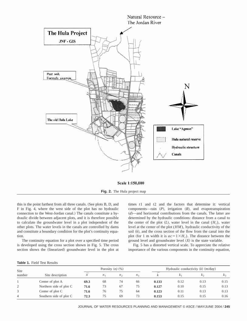
Drainage of the Hula Lake and its surrounding swamps~Figs. 1and 2! by the Jewish National Fund~JNF! in the late 1950s waconsidered a peak of success for the young state of Isralong-standing national dream had been accomplished: the mrampant in the area was eradicated, and the settlers of the Ggained thousands of acres for agricultural use. At the samemeasures were taken to preserve some of the natural and enmental amenities of the area~Shaham 1995!. With time, a seriougap was discovered between the original expectations anactual results. The drained peat soils subsided dramatically,ing spontaneously as the organic matter oxidized and converinfertile ash. Dust storms caused crop damage, and rodentstiplied in burrows in the peat soil and caused severe damacrops. The unique natural amenities of the area were largelyspecies of plant and animal life disappeared, and the numbwater birds diminished. Water quality in the Sea of Galileeaffected by an increased discharge of nitrogen compoundsthe Hula region’s peat soils.

Planning of the Hula restoration project began in the1980s. The first step was to determine the objectives of area

1Faculty of Civil Engineering, Technion-Israel InstituteTechnology.

2Professor, Faculty of Civil Engineering, Technion-Israel InstitutTechnology.

Note. Discussion open until October 1, 2004. Separate discusmust be submitted for individual papers. To extend the closing daone month, a written request must be filed with the ASCE ManaEditor. The manuscript for this paper was submitted for review andsible publication on April 30, 2001; approved on April 25, 2003. Tpaper is part of theJournal of Water Resources Planning and Managment, Vol. 130, No. 3, May 1, 2004. ©ASCE, ISSN 0733-9496/200
243–254/$18.00.
JOURNAL OF WATER RESOURCE

-

and the area resources as guiding principles for the restoplan ~Shaham et al. 1988; Harpaz 1988!. There was consensustwo objectives: preservation of the land value for future gentions, and prevention of water pollution by the Hula peat sThere was controversy regarding restoration of natural valuethe one hand, and on the other, allowing the farming commuwho cultivate the land in the Hula valley to establish sometourism facilities to make up for the income from agriculturewould be lost due to the new project.

Engineering schemes were developed to improve the prtivity of the agricultural land. The main objective of the restotion plan was to raise and maintain a relatively high water tabthe Hula project area, using water from the Jordan River owest side and spring water from the Golan foothills on theside while controlling internal drainage. This was to be accplished by a grid of drainage canals and by careful croppingirrigation. In addition, a small lake, called the Agmon, wformed as a nature reserve and bird refuge. Water levels icanals are controlled by a set of hydraulic structures. Controthe groundwater levels is designed to minimize the decompoand subsidence of the peat soils, ensure year-round green cothe area, and, by avoiding the saturation condition of the cropzone, allow farmers to continue cultivation of their fields~Sha-ham 1995!.

To support the design of the new system, a research anvelopment~R&D! program was initiated by the JNF, includinggeographic information system~GIS! database that stores the sgroundwater, water quality, and engineering infrastructure dathe project. One of the four aims defined in the R&D progra‘‘closing the information and knowledge gap of the local wresources: groundwater and the artificial lake’’~Shaham 1995!. Aspart of the research program, work began on a decision susystem for the Hula project~Ostfeld et al., personal communiction, 1997; De Hoog et al. 1982; Sudicky 1989; Ostfeld e
1999!.
S PLANNING AND MANAGEMENT © ASCE / MAY/JUNE 2004 / 243

dula

of theprovetherge ofrdanby

f the, andalsthe

e thee the. Theis thecingountpear

aluess insbergoutwith

e. Ag 1

ed tog the

waslts are

ions,ven

-

quitethasin the

ojectaller

, theg and

tion,r this

steel

r lev-es ofordsalcu-by thelarmers

t de-entalndenta andpi-

untsn the

thech is

alues

levelsand

blemset ofe con-cond

, ascon-h plotould

enterleastriga-lingd by

hes, the

Decision Support System

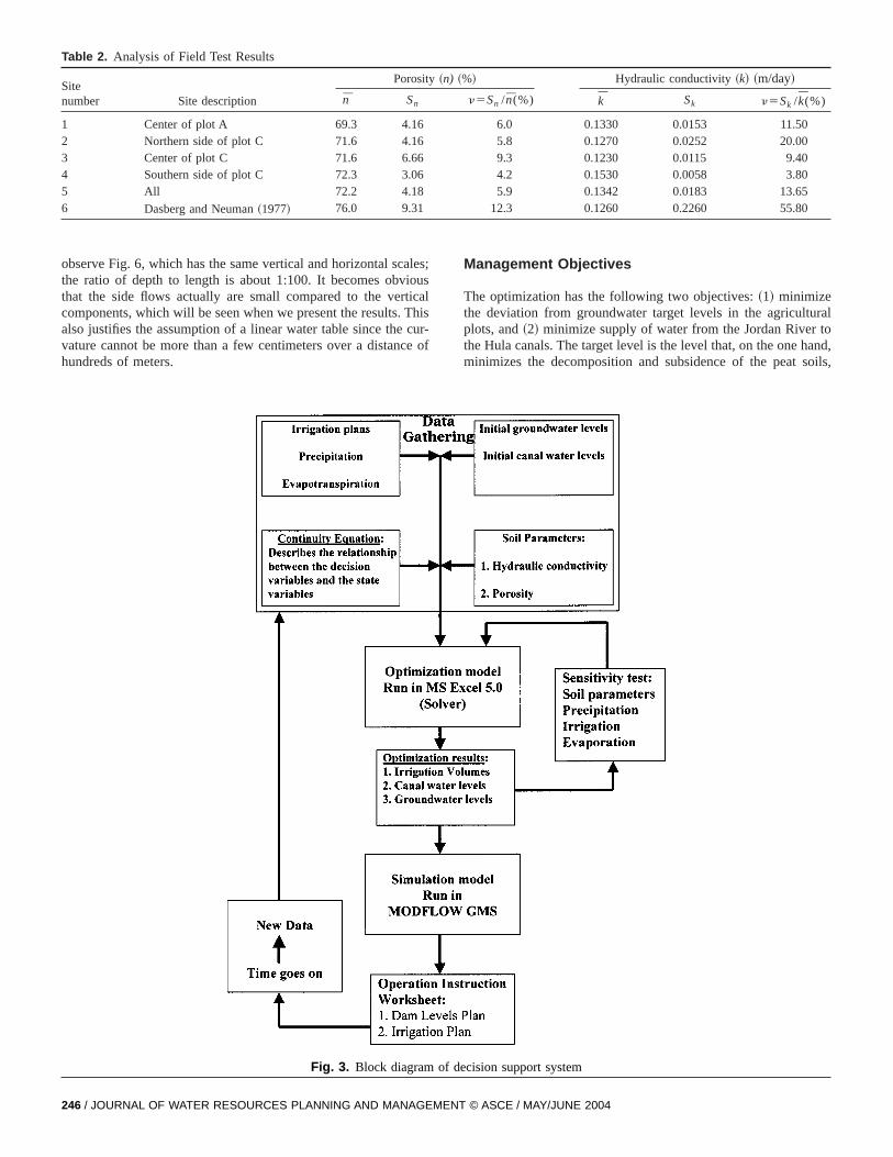
The Hula Decision Support System~HDSS! is designed to aiHula site operators in controlling groundwater levels in the Hregion so as to minimize the decomposition and subsidencepeat soils, ensure year-round green cover of the area, and imagricultural production, thereby contributing to the stability ofland, preserving its value, and reducing the increased dischanitrogen compounds from the Hula region peat soils to the JoRiver, and with it to the Sea of Galilee. This is accomplishedmanagement of the amount of water that flows into and out oarea and controlling water levels in a grid of drainage canalsby the timing and quantity of irrigation. Water levels in the canare controlled by a set of hydraulic structures. By controllingoperation of the Hula project area, the operators can makbest use of the water available locally and thereby reducamount of water that needs to be imported from the outsidesource from which water can be imported to the project areaJordan River, whose waters flow to the Sea of Galilee. Reduimportation of water to the project area thus increases the amavailable for water supply. The components of the HDSS apin Fig. 3.

Data Collection

The hydraulic conductivity~k! and porosity~n! of the soil areimportant parameters in development of the HDSS. These vare difficult to determine due to the highly variable conditionthe field. The parameters were obtained from a study by Daand Neuman~1977! and supplemented by field tests carriedduring this study. These tests were conducted at four sites,three repetitions at each site, using the following procedur12-in. pipe was inserted vertically to a depth of 3.5 m, leavinm of pipe above the ground level. Slug tests were then uscalculatek. Porosity was also measured at the same sites usin

Fig. 1. Location map

following procedure: undisturbed soil samples were obtained

244 / JOURNAL OF WATER RESOURCES PLANNING AND MANAGEMENT

from a depth of 1 to 1.2 m using 6-in. PVC pipe, and porositythen determined by saturating the dried samples. The resugiven in Table 1, together with the average for each site~over thethree repetitions!. Table 2 gives the averages, standard deviatand relative variations~the latter are considered valuable ethough the number of samples is small!. The results are also compared to those of Dasberg and Neuman~1977!.

The average values obtained in the field experiment aresimilar to those in Dasberg and Neuman~1977!. The somewhalower values ofn may be due to additional subsidence thatoccurred since 1977. Table 2 shows a substantial differencevariability of the results. Dasberg and Neuman~1977! performedtheir tests in many different areas throughout the Hula prarea, while in the present study tests were performed in a smpart. Accordingly, the results seem more uniform. Thereforevalues used in this work are the values obtained by DasberNeuman~1977!.

Data on canal water levels, groundwater levels, precipitairrigation, and evapotranspiration were recorded weekly. Fopurpose, four observation wells made of perforated stainlesstubes were inserted into the ground to a depth of 4 m at thesamefour sites where soil parameters were measured. Canal wateels were measured at 18 hydraulic structures and eight nodthe canals. The meteorology station of the Hula project recprecipitation and evaporation data and then transpiration is clated. These data are gathered and analyzed for the farmersNorth Galilee Laboratory~MIGAL ! and provided to the Huproject operators. Using the evapotranspiration data, the fadetermine the irrigation amounts required.

System Equations

There are two possible ways to construct the equations thascribe the system. One is to use field data and find experimfunctional relationships between the independent and depevariables. The independent variables are the external datcontrol variables~for example, precipitation, evaporation, transration, and water levels in the canals, and irrigation amo!while the dependent variables are the groundwater levels iplots. This approach would alleviate the need to determinesoil parameters, which are highly variable. The other approato use the continuity equation for each plot and insert the vof parameters~that is, geometry and soil properties!. The firstapproach failed, since the measurements of groundwaterthroughout the Hula Valley are not sufficiently dense in spacetime and are sometimes inconsistent. Therefore, due to proin the field data, it was not possible to obtain a consistent ssystem equations based on data, and we had to resort to thtinuity approach. The HDSS is therefore based on the seapproach.

A network of canals that surround the agricultural plotsshown schematically in Fig. 4, divides the project area. Thetrol scheme uses the groundwater level at the center of eacas the control variable, based on the assumption that this wresult in an adequate level throughout the entire plot. The cof the plot is the farthest point from the canals and thereforeaffected by canal water levels, but is the most affected by irtion, which turned out to be the dominant factor in controlgroundwater levels. The results of the optimization were testesimulation ~Fig. 3!, and the results verified the validity of tassumption. When a plot is surrounded from only three side
representative point is in the middle of the side without a canal, as
© ASCE / MAY/JUNE 2004

dulicy-siblef theams

qua-

riodcrossat

calnare

al to

ethe

he

lativetion,

this is the point farthest from all three canals.~See plots B, D, anF in Fig. 4, where the west side of the plot has no hydraconnection to the West-Jordan canal.! The canals constitute a hdraulic divide between adjacent plots, and it is therefore posto calculate the groundwater level in a plot independent oother plots. The water levels in the canals are controlled by dand constitute a boundary condition for the plot’s continuity etion.

The continuity equation for a plot over a specified time peis developed using the cross section shown in Fig. 5. Thesection shows the~linearized! groundwater level in the plot

Fig. 2. The

Table 1. Field Test Results

Sitenumber Site description

Porosity~n) ~

n̄ n1

1 Center of plot A 69.3 68

2 Northern side of plot C 71.6 73

3 Center of plot C 71.6 76

4 Southern side of plot C 72.3 75


times t1 and t2 and the factors that determine it: verticomponents—rain~P!, irrigation ~R!, and evapotranspiratio~d!—and horizontal contributions from the canals. The latterdetermined by the hydraulic conditions: distance from a canthe center of the plot~L!, water level in the canal (Hc), waterlevel at the center of the plot (HM ), hydraulic conductivity of thsoil ~k!, and the cross section of the flow from the canal intoplot ~for 1 m width it is ac513Hc). The distance between tground level and groundwater level~X! is the state variable.

Fig. 5 has a distorted vertical scale. To appreciate the reimportance of the various components in the continuity equa

project map

Hydraulic conductivity~k! ~m/day!

n3 k̄ k1 k2 k3

66 0.133 0.12 0.13 0.15

75 0.127 0.10 0.15 0.13

64 0.123 0.11 0.13 0.13

73 0.153 0.15 0.15 0.16

Hula

%!

n2

74

67

75

69


cales;ious

rtical. This

cur-ce of

turalto

hand,soils,

observe Fig. 6, which has the same vertical and horizontal sthe ratio of depth to length is about 1:100. It becomes obvthat the side flows actually are small compared to the vecomponents, which will be seen when we present the resultsalso justifies the assumption of a linear water table since thevature cannot be more than a few centimeters over a distanhundreds of meters.

Table 2. Analysis of Field Test Results

Sitenumber Site description

Porosit

n̄ Sn

1 Center of plot A 69.3 4.162 Northern side of plot C 71.6 4.13 Center of plot C 71.6 6.664 Southern side of plot C 72.3 3.05 All 72.2 4.186 Dasberg and Neuman~1977! 76.0 9.31

Fig. 3. Block diagram


Management Objectives

The optimization has the following two objectives:~1! minimizethe deviation from groundwater target levels in the agriculplots, and~2! minimize supply of water from the Jordan Riverthe Hula canals. The target level is the level that, on the oneminimizes the decomposition and subsidence of the peat

! Hydraulic conductivity~k! ~m/day!

n5Sn /n̄(%) k̄ Sk n5Sk / k̄(%)

6.0 0.1330 0.0153 11.505.8 0.1270 0.0252 20.009.3 0.1230 0.0115 9.404.2 0.1530 0.0058 3.80

5.9 0.1342 0.0183 13.6512.3 0.1260 0.2260 55.80

ecision support system

y~n) ~%

6

6

of d


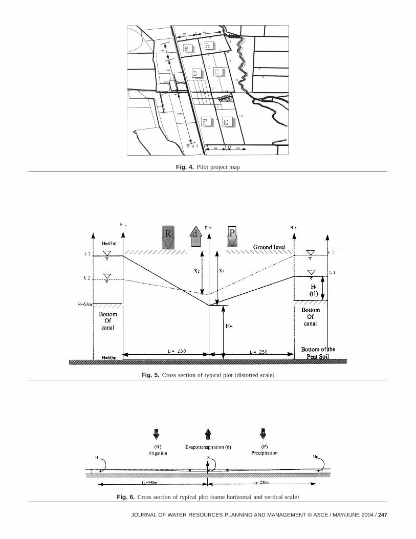
Fig. 4. Pilot project map

Fig. 5. Cross section of typical plot~distorted scale!

Fig. 6. Cross section of typical plot~same horizontal and vertical scale!

JOURNAL OF WATER RESOURCES PLANNING AND MANAGEMENT © ASCE / MAY/JUNE 2004 / 247

n ofdanicu-

thatater

tripx

endlot;

l;

ol-d of

hgh

h

t;

h

-i-

l;

o thetion

t

7:

tes. Aswateror intoelowricul-riodsr

and on the other hand, allows farmers to continue cultivatiotheir fields. Minimizing water import to the area from the Joris in recognition of the scarcity of water in that region, partlarly in summer. The second objective is designed to ensurethe project will import the least amount of water, since wquantity in this area is limited.

Constraints: Continuity Equations

The continuity equations are formulated for a 1-m wide sacross the plot between the canal on the left~denoted by the indeL! and the one on the right~denoted byR! for a time periodDt,from t1 to t2.

The change in water volume between the beginning~super-script 1! and end~superscript 2! of the period is

DV5 H LL

2@~HL

21HM2 !2~HL

11HM1 !#1

LR

2@~HR

21HM2 !

2~HR11HM

1 !#J •n (1)

whereDV5change in water volume between beginning andof period; LR5distance between right canal and center of pLL5distance between left canal and center of plot;HR5waterlevel in right canal; HL5water level in left canaHM5groundwater level at center of plot; andn5soil porosity.

QVolume5DV

Dt(2)

whereQvolume5discharge to plot calculated from change in vume;DV5change in water volume between beginning and enperiod; andDt5time between beginning and end of period.

Dt5t22t1 (3)

whereDt5time between beginning and end of period;t15time atbeginning of period; andt25time end of period.

The flow entering/exiting from/to the left canal is

QL5F12 ~HL11HL

22HM1 2HM

2 !G• 1

LL•aL•k5DHL•

1

LL•aL•k

(4)

whereQL5discharge to plot from left canal;HL5water level inleft canal;HM5groundwater level at center of plot;LL5distancebetween left canal and center of plot;aL5area through whicflow occurs; andk5hydraulic conductivity. The area throuwhich the flow occurs is

aL5HL31m (5)

whereHL5water level in left canal; andaL5area through whicflow occurs. Similarly, flow from/to right canal is

QR5F12 ~HR11HR

22HM1 2HM

2 !G• 1

LL•aR•k5DHR•

1

LR•aR•k

(6)

whereQR5discharge to plot from right canal;HR5water level inright canal; HM5groundwater level at center of ploLR5distance between right canal and center of plot;aR5areathrough which flow occurs; andk5hydraulic conductivity.

aR5HR31m (7)

where HR5water level in right canal; andaR5area throug
which flow occurs.

The total net inflow from above is

Qt5~DR1DP2Dd!•A (8)

whereDP5rate of recharge from precipitation~depth of precipitation divided by time interval!; DR5rate of recharge from irrgation;Dd5rate of evapotranspiration; andA5(LL1LR)31 sur-face area of strip.

The total net inflow during the time interval is

Qflow5QL1QR1QI (9)

whereQflow5total net inflow during time interval;QL5dischargeto plot from left canal;QR5discharge to plot from right canaandQi5total net inflow from above.

The change in the water volume in the ground is equated tinflux calculated by the flow equation. The continuity equafor plot i is

QFi 5(

cQc

i 1QIi (10)

whereQF5total flow to plot I; (cQc5sum of flow from all ofcanal to plotI; andQi5total net inflow from above to ploti.

DSti5QF

i (11)

whereDSi5change in water storage plotI; andQFi5total flow toplot i.

hGi 2ht21

i 1Dhti5xt

i (12)

wherehGi 5ground level in plotI; ht

i5groundwater level in plotiduring time periodt; ht21

i 5groundwater level in ploti duringtime periodt21; andxt

i5groundwater depth at center of ploiduring time periodt.

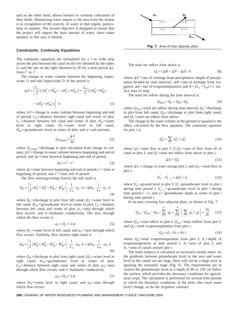
In an area covering four adjacent plots, as shown in Fig.

Qin2Qout2Qd5(i 51

4

qFi 5(

i 51

4 S (c

qci 1qI

i D 5ds

dt(13)

whereQin5total inflow to plot I; Qout5total outflow from plotI;andQd5total evapotranspiration from ploti.

Qd5dt•~Ai1Ac! (14)

where Qd5total evapotranspiration from plotI; dt5depth ofevapotranspiration at time periodt; Ai5area of plot I; andAc5area of canals around ploti.

The water balance is calculated as successive steady stathe gradients between groundwater level in the area andlevel in the canals are not large, there will not be a large errignoring the transition stage~Fig. 6!. The requirements arecontrol the groundwater level at a depth of 80 to 150 cm bthe surface, which provides the necessary conditions for agtural crops. The calculation is performed for several time pein which the boundary conditions of the plots~the canal wate

Fig. 7. Area of four adjacent plots

level! change, as do the irrigation volumes.


of aith

rap-del

llingis a

th aom-with

f theent oed onsys-

forthe

area,ela-infor-ubar-oduleram-The

f

avior

ioneri-pointt theouldessaThe

0 andm atthedernc-

velsre is

ly asd isuslyion

ofveral

s;of-;

on;l

epor-.to setght/

n theince994.data

bareanaling theg therauli-areanveypilotthe

plef theolver-Aus-

in-the

d by

tiveri-

sheet

lesalso

andThey

Management Module

The operational plan can be developed for the entire lengthsingle growing season, which is typically up to 4 months, wweekly time intervals. In fact, since conditions change quiteidly, and to maintain model simplicity for practical use, the mois developed for a period of 8 weeks and is run on a rowindow. This means that the model is rerun every time therechange in conditions, typically once every 2 to 3 weeks, witime horizon of 8 weeks ahead. The weekly time interval is cpatible with the operational schedule in the field, as well asthe rate of change in canal and groundwater levels.

For demonstration, the model was developed for a part ooverall area that can be considered separate and independthe neighboring areas. The division into such subareas is basanalysis of the groundwater level maps obtained with a GIStem that uses field observations.

From a visual analysis of groundwater maps using a GISthe Hula project, one can identify four or five subareas inproject according to groundwater level behavior. In each subthe groundwater level is relatively uniform, while there is a rtively large difference between the subareas. Based on thismation, it seems best to divide the entire project area into seas, allowing each subarea to have its own management mwith its geographic/geometric data and its specific ground paeters. The modules for the subareas are run in parallel.boundaries of the subareas are clear landmarks~the old channel othe Jordan River, Lake Agmon, topographic differences! thatseparate the subareas in terms of their hydrological beh~Fig. 2!.

The first objective of the optimization is to minimize deviatof the groundwater level from the target level over all time pods. The target level is the desired groundwater level at anyin time. In setting the target level one must take into accounage of a crop and the depth of its roots. The groundwater shbe as close as possible to the surface and yet leave the necdistance for plant growth between the roots and the water.Hula restoration plan defines the desired level as between 8150 cm from the surface—80 cm in the summer and 150 cthe beginning of winter. The second objective—minimizingtotal quantity of water supplied to the area unconsideration—is achieved indirectly by the first objective fution. The demand for minimum deviation from the target leleads to supply of water from the Jordan River only when thea deficit in the area~levels are below the target values! during thefirst weeks in order to reach the desired target level as quickpossible. The water demand for the rest of the time periominimal. If the second objective is not achieved simultaneowith the first, it is possible to use a multiobjective optimizatapproach. The objective function is minimization of the sumsquares of the deviations from the target levels, subject to setypes of constraints:

Minhi

c,Ri; i ,c

(i 51

N

b i•~Xi2Xtarget!2 (15)

subject to 80 cm<Xi<150 cm; HupIstream>HdownIstream; (hground

22.5)<hic<hground; Hc at canal junction equal in all direction

0<Ri ; and 0<b i<1; whereXi5groundwater depth at centerplot I; Xtarget5target for groundwater depth;b i5importance factor of plot I; Ri5water input to plot I from above
HupIstream5water level in upstream canal in junction;

f

ry

HdownIstream5water level in a downstream canal in a junctihground5ground level above sea level; andhi

c5canal water leveabove sea level.

The objective function is nonlinear. Sinceb i is the importancfactor of plot i in the subarea, at the calibration stage the imtance of all plots is assumed equal, and sob i51 for all the plotsWhen calibrating the module for each subarea, it is possiblethe b coefficient for each plot so as to reflect the weiimportance of each plot.

Pilot Project

The management module in this work is for one subarea iHula project, as shown in Fig. 4. It is called the pilot project sthe first operational experiments were performed here in 1The data collected in those early experiments, and furthercollected for the present study, were used herein. The sucontains the following six plots: A, B, C, D, E, and F. Casegments between operational dams in the canals surroundplots were numbered 1 to 18. The boundary on the west, alonWest-Jordan canal, is impervious and is not connected hydcally to the pilot project area. To the east of the pilot projectis the old Jordan River, which is used as the main canal to cowater to the entire Hula area. It also supplies water to theproject through canal number 1. The pilot project is drained tosouth, through canal 18 to a reservoir.

Optimization

MS-Excel is used to perform the optimization. This is a simand well-known software package that facilitates the use oDSS by the Hula project operators. The algorithm used by Sis the Generalized Reduced Gradient~GRG2! nonlinear optimization code developed by Leon Lasdon, University of Texas attin, and Allan Waren, Cleveland State University. Linear andteger problems use the simplex method with bounds onvariables, and the branch-and-bound method, implementeJohn Watson and Dan Fylstra, Frontline Systems, Inc.~VisualBasic User’s Guide, Microsoft Excel, Microsoft Corp.!.

The setup of the optimization is according to the objecfunction in Eq.~15!. The Pilot Project Model has 23 control vaables and 6 dependent variables.

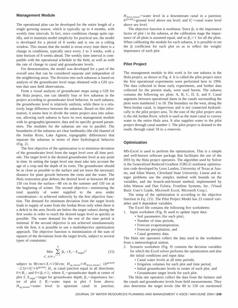
The Excel file contains the following five worksheets:1. Input worksheet~Fig. 8! used to update input data:

• Soil parameters~for each plot!,• Number of time periods,• Forecast evapotranspiration,• Forecast precipitation, and• Canal geometry data.

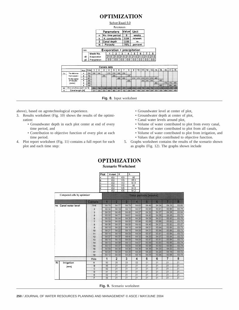
The Hula site operators collect the data used in the workfrom a meteorological station.2. Scenario worksheet~Fig. 9! contains the decision variab

for which the Excel solver performs the optimization andthe initial conditions and input data:

• Canal water levels at all time periods,• Irrigation volumes for each plot and time period,• Initial groundwater levels in center of each plot, and• Groundwater target levels for each plot.

The Hula site operators collect the data from the farmersthe canals and groundwater levels from field measurements.
also determine the target levels~the 80 to 150 cm mentioned

i-

very

ch

h

l,

nd

hown

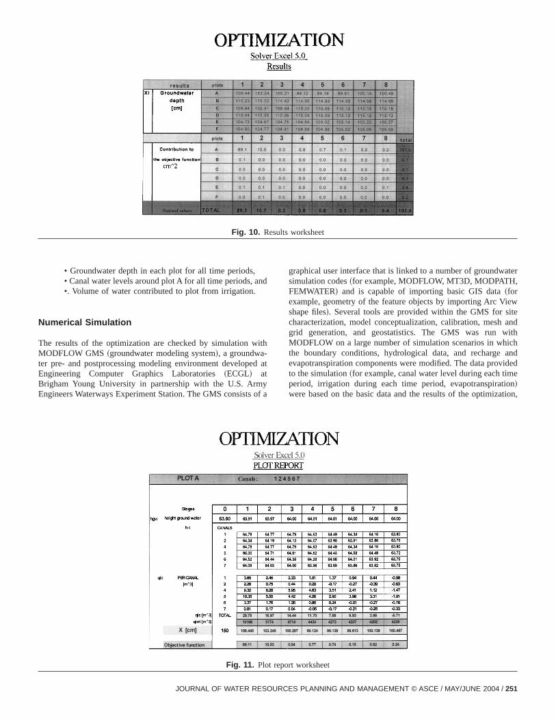
above!, based on agrotechnological experience.3. Results worksheet~Fig. 10! shows the results of the optim

zation:• Groundwater depth in each plot center at end of e

time period, and• Contribution to objective function of every plot at ea

time period.4. Plot report worksheet~Fig. 11! contains a full report for eac

plot and each time step:

Fig. 8. In

Fig. 9. Sc


• Groundwater level at center of plot,• Groundwater depth at center of plot,• Canal water levels around plot,• Volume of water contributed to plot from every cana• Volume of water contributed to plot from all canals,• Volume of water contributed to plot from irrigation, a• Values that plot contributed to objective function.

5. Graphs worksheet contains the results of the scenario sas graphs~Fig. 12!. The graphs shown include

orksheet

worksheet

put w

enario


and

with-ed at

myof a

ater,

iewiteand

withichand

videdimetionation,

• Groundwater depth in each plot for all time periods,• Canal water levels around plot A for all time periods,•. Volume of water contributed to plot from irrigation.

Numerical Simulation

The results of the optimization are checked by simulationMODFLOW GMS ~groundwater modeling system!, a groundwater pre- and postprocessing modeling environment developEngineering Computer Graphics Laboratories~ECGL! atBrigham Young University in partnership with the U.S. ArEngineers Waterways Experiment Station. The GMS consists

Fig. 10. R

Fig. 11. Plo


graphical user interface that is linked to a number of groundwsimulation codes~for example, MODFLOW, MT3D, MODPATHFEMWATER! and is capable of importing basic GIS data~forexample, geometry of the feature objects by importing Arc Vshape files!. Several tools are provided within the GMS for scharacterization, model conceptualization, calibration, meshgrid generation, and geostatistics. The GMS was runMODFLOW on a large number of simulation scenarios in whthe boundary conditions, hydrological data, and rechargeevapotranspiration components were modified. The data proto the simulation~for example, canal water level during each tperiod, irrigation during each time period, evapotranspira!were based on the basic data and the results of the optimiz

worksheet

rt worksheet

esults

t repo


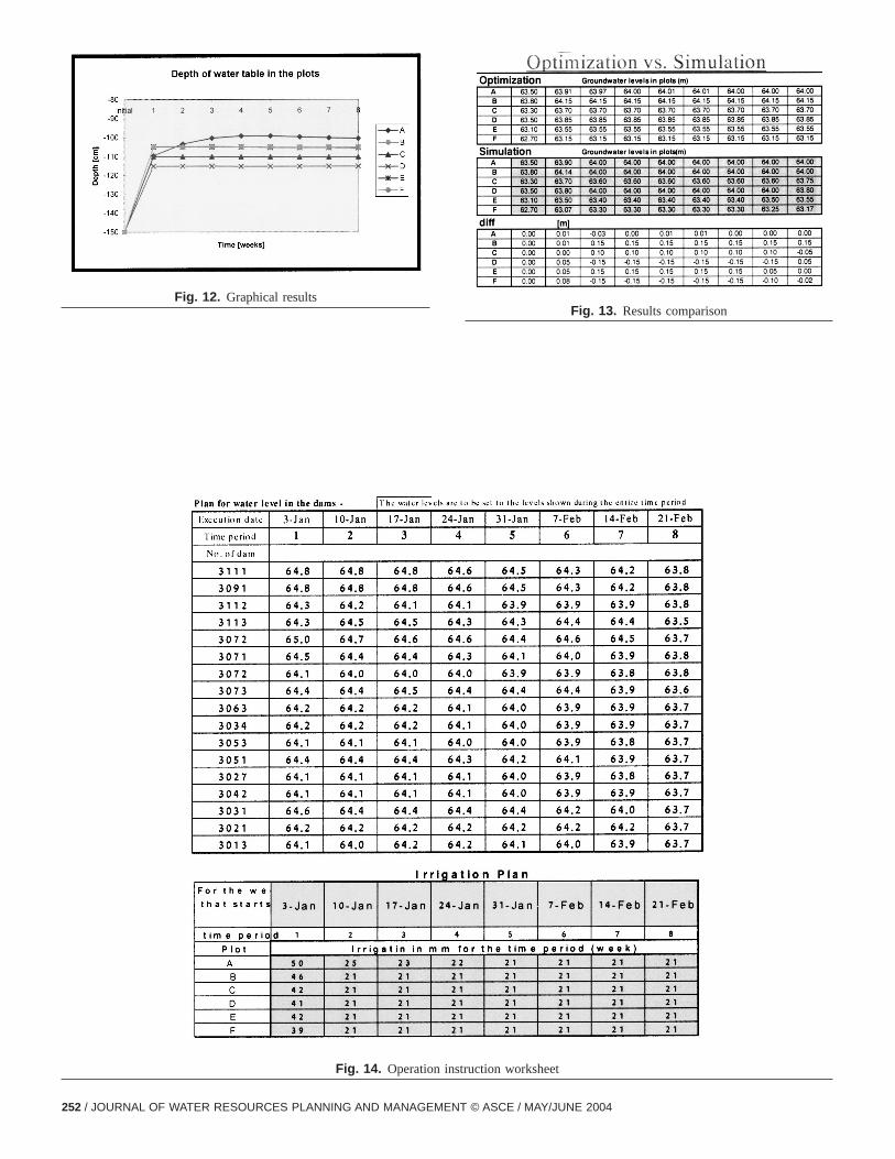
Fig. 12. Graphical results


Fig. 13. Results comparison

Fig. 14. Operation instruction worksheet


MScellyer

andctione isthe

edruct-to thererun

ucesntrolched-ork-

inalu-

e

gh

lev-waterch

050

igh,3 ton isthefill-

rios,ualsffer-r-her toe

con-the

longtion,eeksthehighitiesikelyly itn the

es itstargetolu-fromon in

at areoject

ision. In

ecise

d re-ol theca-

in then thattuallyrtantrop-sec-

ct

oreithhileTheverlyun-bal-

which are arranged in a specific data file format for the Goptimization results. The saturated zone is modeled with asize of 403120 m and a depth of 6 m, equal to the peat soil ladepth.

Management Module

The module provides a comparison between the simulationoptimization results and preparation of an operation instruworksheet. At the end of the simulation, the GMS output filconverted to an EXCEL file for comparison with the results ofoptimization ~Fig. 13!. If the differences are within a specifitolerance~65%!, the optimization results are used to constthe operation instruction worksheet~Fig. 14!. When the differences are significant, it is necessary to check the input datasimulation or use the sensitivity test to refine the data andthe model.

Operation Instruction Worksheet

After confirmation of the results, the user of the HDSS proda worksheet to instruct the Hula site operators how to cocanal water levels by managing the dams and the irrigation sule during the planning period. An example to the two-part wsheet is shown in Fig. 14.

Computational Results and Analysis

Three main variables that affect the results are~1! initial ground-water levels in the plots;~2! target levels for the groundwaterthe plots; and~3! evapotranspiration. These variables are evated under two extreme scenarios:~1! a filling scenario, whichstarts with low groundwater levels~that is, 2.00 m below thsurface! and ends with high groundwater levels~that is, 0.60 to1.00 m!; and ~2! emptying scenario, which starts with higroundwater levels~that is, 0.60 to 1.00 m! and ends with lowgroundwater levels that match the requirement for minimumels to be 1.50 m below the surface. As explained earlier, thebalance is calculated for a series of~quasi! steady states. Eascenario is run for three conditions of evapotranspiration:~1! high~28 to 30 mm/week!; ~2! low ~7 to 10 mm/week!; and~3! highlyvariable during the planning period~varying between 15 and 3mm/week!. In all cases the maximum irrigation allowed wasmm/week.

Analysis

1. For the filling scenarios, when the evapotranspiration is hthe process of filling to target groundwater level requires4 weeks in most of the plots. When evapotranspiratiolow, the filling process takes only 1 to 2 weeks, and whenevapotranspiration varies during the planning period, theing process extends over 2 weeks. In all the filling scenaafter reaching the target level, the irrigation quantity eqevapotranspiration in most of the plots. In some plots, dient boundary conditions~for example, the number of surounding canals! and/or the topographic conditions of tplot ~for example, the upstream canals contribute watethe upper and lower plots as well! affects the length of tim
required for filling the plot area.

2. For the emptying scenarios, the emptying process istrolled largely by the amount and rate of drainage fromplot to the canals. This is a long process due to thedrainage path. For the scenario with low evapotranspirathe results indicate that the drainage requires about 5 wwith no irrigation, and after reaching the target levelirrigation equals evapotranspiration. For a scenario withevapotranspiration, irrigation is required in smaller quantthan is evapotranspiration. The emptying process is unlto occur in periods with high evapotranspiration; usualoccurs before the winter, when preparations are made iHula Valley for the rainy season.

Conclusions

The optimizer seeks a solution where groundwater reachtarget level as rapidly as possible and then maintains theclose to this level until the end of the planning period. This stion always leads to minimum release of water downstreamthe project area, and therefore to minimum water consumptithe project area~this is the second objective!. The optimizationmodel developed in this work provides reasonable results thcompatible with the accumulated experience of the Hula properators.

The accuracy of the model matches the operational precof the dams in the canal network and the irrigation systemplots where this is not the case, it is possible to run a more prsimulation with GMS to obtain more detailed results.

Prior to the analysis described here, both operators ansearchers believed that most of the water needed to contrgroundwater levels is provided laterally to the plots from thenals. For this reason, there has been a major investmentcanal network and its controls. The present study has showmost of the water needed to raise groundwater levels is acsupplied to the plots from irrigation, and the canals are impomostly as boundary conditions to prevent the levels from dping. This becomes quite evident when examining the crosstion of the plot in true scale~Fig. 6! rather than the abstradiagram shown in Fig. 3.

As a result of this study, the operators are investing mattention and time in planning the irrigation program jointly wthe farmers in a way that will meet the needs of the crops wkeeping the groundwater levels within the desired range.model is also used to understand why certain plots become odry or wet under certain conditions. It also helps to identifyderground preferential flow paths and to calculate the waterance in plots and in the entire project more accurately.

Notation

The following symbols was used in this paper:A 5 (LL1LR)* 1 surface area of strip~m2!;

Ac 5 area of canals around ploti (m2);Ai 5 area of ploti (m2);aL 5 area through which left flow occurs~m2!;aR 5 area through which right flow occurs~m2!;dt 5 depth of evapotranspiration at time period

t (mm);HdownIstream 5 water level in downstream canal in junction

~m!;
HL 5 water level in left canal~m!;

a

.

ntal

in

Arans-

HM 5 groundwater level at center of plot~m!;HR 5 water level in right canal~m!;

HupIstream 5 water level in upstream canal in junction~m!;

hground 5 ground level above sea level~m!;hi

c 5 canal water level above sea level~m!;hG

i 5 ground level in ploti (m);ht

i 5 groundwater level in ploti during timeperiod t (m);

ht21i 5 groundwater level in ploti during time

period t21 (m);k 5 hydraulic conductivity~m/h!;

LL 5 distance between left canal and center ofplot ~m!;

LR 5 distance between right canal and center ofplot ~m!;

n 5 soil porosity~%!;Qd 5 total evapotranspiration from plot~m3/h!;

QFi 5 total flow to plot i (m3/h);Qflow 5 total net inflow during time interval~m3/h!;

Qi 5 total net inflow from above~m3/h!;Qin 5 total inflow to plot i (m3/h);QL 5 discharge to plot from left canal~m3/h!;

Qout 5 total outflow from ploti (m3/h);QR 5 discharge to plot from right canal~m3/h!;

Qvolume 5 discharge to plot calculated from change involume ~m3/h!;

Ri 5 water input to plotI from above~mm!;Xi 5 groundwater depth at center of ploti (m);

X 5 target for groundwater depth~m!;
target

xti 5 groundwater depth at center of ploti during

time periodt (m);b i 5 importance factor of ploti;

Dd 5 rate of evapotranspiration~mm/h!;DP 5 rate of recharge from precipitation~mm/h!;DR 5 rate of recharge from irrigation~mm/h!;DSi 5 change in water storage ploti (m3);Dt 5 time between beginning and end of period

~h!;DV 5 change in water volume between beginning

and end of period~m3!; and(cQc 5 sum of flow from all canal to ploti (m3/h).

References

Dasberg, S., and Neuman, S. P.~1977!. ‘‘Peat hydrology in the HulBasin, Israel. I: Properties of peat.’’J. Hydrol.,32, 219–239.

De Hoog, F. R., Knight, J. H., and Stokes, A. N.~1982!. ‘‘An improvedmethod for numerical inversion of Laplace transform.’’SIAM (SocInd. Appl. Math.) J. Sci. Stat. Comput.,3~3!, 357–366.

Harpaz, A.~1988!. The drainage of the Hula Valley and its environmeconsequences, Dept. of Geography, Haifa Univ.~in Hebrew!.

Ostfeld, A., Muzaffar, E., and Lansey, E. K.~1999!. ‘‘Analytical ground-water flow solutions for channel-aquifer interaction.’’J. Irrig. Drain.Eng.,125~4!, 196–202.

Shaham, G.~1995!. ‘‘Hula project—Dynamic of human interferencenature.’’Ecology and Environment,221–224~in Hebrew!.

Shaham, G., Mintzker, H., and Kenahan, G.~1988!. ‘‘Alternatives for theuse of the Hula Valley land.’’Feasibility study~in Hebrew!.

Sudicky, E. A. ~1989!. ‘‘The Laplace transform Galerkin technique:time-continuous finite element theory and application to mass tport in groundwater.’’Water Resour. Res.,25~8!, 1833–1846.


Documents

Managing Groundwater Levels in an Agricultural Area with