Magnetic surveys - University of British Columbia · Magnetic surveys Geophysical magnetic surveying makes use of the fact that Earth's magnetic field causes, or induces, subsurface

Magnetic surveys

Introduction

This large learning resource concentrates on background about using Earth's magnetic field to learn about its subsurface.Practicalities of interpreting maps, profiles, or inversion models are not discussed.

Magnetic surveys

Geophysical magnetic surveying makes use of the fact that Earth's magnetic field causes, or induces, subsurface materials to become magnetized. Referring to the following three-component outline, all applied geophysics problems can be discussed interms of a source of energy that is put into the ground, the effects on that energy due to subsurface variations in the relevantphysical property, and the measurements that detect those changes to the input energy. Signals are interpreted in terms of thesubsurface distribution of the physical property, which in the case of magnetic surveys is magnetic susceptibility.

Using the same colour scheme as the figure above, Figures 2a - 2e illustrate how this concept applies to magnetic surveys. In thiscase, the energy source is Earth's global magnetic field (Figure 2a) which has a strength and direction at every location on theEarth (Figure 2b). Subsurface materials (Figure 2c) become magnetized by this field (Figure 2d), and the data (Figure 2e) willinvolve measurements of the magnetic field at the Earth's surface, in the air, in space, or within boreholes. The measuredmagnetic field will be a superposition of Earth's field and the induced secondary fields caused by magnetization of buriedmaterials.

2a. Earth's magnetic field. 2b. It has strength and direction

everywhere.

2c. No incident magnetic field. 2d. Earth's field causes

material to become magnetized.

2e. Data are a superposition of Earth's field and resulting induced

fields.

The physical property - susceptibility

Earth materials contain magnetic particles. Generally these are oriented in random directions and they produce no overall

magnetic field (Figure 3a). However, when subject to an inducing field such as Earth's natural magnetic field, H0, these particles

will align themselves and the material will become magnetized (Figure 3b). The strength of that induced magnetization, M,

depends upon the magnetic susceptibility, K, of the material. In fact, the strength of this induced magnetization field is M=KH0.

Note that M and H0 are vector quantities and K is a scalar value - the physical property of the material.

3a. 3b.

In the field, the superposition of natural and induced fields is measured because they exist together. In general, after a magnetic

survey is completed, the natural and induced fields are separated; then the residual induced (or anomalous) magnetic field isinterpreted in terms of the magnitude and distribution of susceptible material under the ground. The resulting model of subsurfacesusceptibility must then be interpreted in terms of useful geologic and geotechnical parameters (rock types, structures, buriedobjects, etc.).

Some materials retain a natural permanent or "remanent" magnetization. This is a third component of measurable magnetic fieldswhich complicates the interpretation of magnetic surveys because there is no way to separate the induced and remanentcomponents. All content in this resource assumes remanent magnetization is zero, but this is usually not the case.

More details about the magnetic susceptibility of geological materials (and remanent magnetization) are given in a separate AGLOresource about magnetic susceptibility.

Typical problems where magnetics is useful

Geologic mapping using ground or airborne magnetic data.Ore body characterization (location, depth, volume, mineral composition).Geotechnical (finding and mapping utilities and geologic materials or structures).Archeological object and feature mapping.Mapping continental scale geologic structure.Planetary scale investigations from satallite platforms (Earth, Mars, etc.).Paleomagnetics (sea floor spreading and rock dating).

F. Jones, UBC Earth and Ocean Sciences, 01/10/2007 19:30:20

Measurements for magnetic surveys

Measurements

What exactly is measured during a magnetics survey? Any measurement of Earth's field, whether it includes effects of inducedfields or not, involves measuring vector quantities. Most surveys record the magnitude of the combination of all fields at thelocation of the sensor. Sometimes the magnitude is measured in a specific direction (the vertical component of the combinedfields, for example), and sometimes the gradient is measured as a difference in field strength at two locations a few metres apart.

Regardless of which type of measurement is involved, the quantity that is recorded is a combination of the amount due to Earth'sfield, and the amounts due to all fields induced by the Earth's field. The concept is illustrated in the interactive Figures 1 through19 below. Details about the expected measurements on a surface above buried magnetic objects are outlined next.

Move your mouse over the links and read the captions.

Magnetic fields over a uniform Earth.

Induction: Earth's field causes

induced fields.

Vector addition gives the total

result.

The result depends upon location.

Figure 1 Figure 2 Figure 3 Figure 4

Figure 5 Figure 6 Figure 7 Figure 8 Figure 9 Figure 10 Figure 11

Figure 12Figure 13Figure 14Figure 15

Figure 16Figure 17Figure 18Figure 19


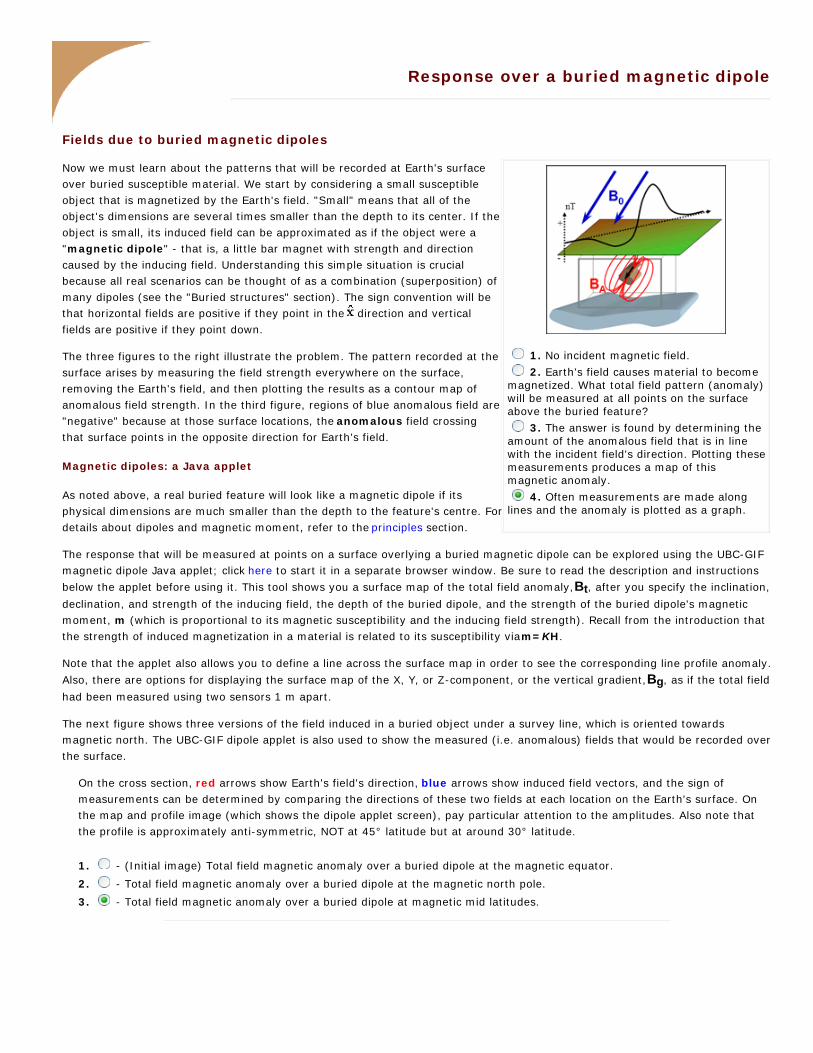
1. No incident magnetic field.

2. Earth's field causes material to become magnetized. What total field pattern (anomaly)will be measured at all points on the surface above the buried feature?

3. The answer is found by determining the amount of the anomalous field that is in line with the incident field's direction. Plotting thesemeasurements produces a map of this magnetic anomaly.

4. Often measurements are made along lines and the anomaly is plotted as a graph.

Response over a buried magnetic dipole

Fields due to buried magnetic dipoles

Now we must learn about the patterns that will be recorded at Earth's surfaceover buried susceptible material. We start by considering a small susceptibleobject that is magnetized by the Earth's field. "Small" means that all of theobject's dimensions are several times smaller than the depth to its center. If theobject is small, its induced field can be approximated as if the object were a "magnetic dipole" - that is, a little bar magnet with strength and directioncaused by the inducing field. Understanding this simple situation is crucialbecause all real scenarios can be thought of as a combination (superposition) ofmany dipoles (see the "Buried structures" section). The sign convention will bethat horizontal fields are positive if they point in the direction and vertical fields are positive if they point down.

The three figures to the right illustrate the problem. The pattern recorded at thesurface arises by measuring the field strength everywhere on the surface,removing the Earth's field, and then plotting the results as a contour map ofanomalous field strength. In the third figure, regions of blue anomalous field are"negative" because at those surface locations, the anomalous field crossingthat surface points in the opposite direction for Earth's field.

Magnetic dipoles: a Java applet

As noted above, a real buried feature will look like a magnetic dipole if itsphysical dimensions are much smaller than the depth to the feature's centre. Fordetails about dipoles and magnetic moment, refer to the principles section.

The response that will be measured at points on a surface overlying a buried magnetic dipole can be explored using the UBC-GIFmagnetic dipole Java applet; click here to start it in a separate browser window. Be sure to read the description and instructions

below the applet before using it. This tool shows you a surface map of the total field anomaly, Bt, after you specify the inclination,

declination, and strength of the inducing field, the depth of the buried dipole, and the strength of the buried dipole's magneticmoment, m (which is proportional to its magnetic susceptibility and the inducing field strength). Recall from the introduction thatthe strength of induced magnetization in a material is related to its susceptibility via m=KH.

Note that the applet also allows you to define a line across the surface map in order to see the corresponding line profile anomaly.

Also, there are options for displaying the surface map of the X, Y, or Z-component, or the vertical gradient, Bg, as if the total field

had been measured using two sensors 1 m apart.

The next figure shows three versions of the field induced in a buried object under a survey line, which is oriented towardsmagnetic north. The UBC-GIF dipole applet is also used to show the measured (i.e. anomalous) fields that would be recorded overthe surface.

On the cross section, red arrows show Earth's field's direction, blue arrows show induced field vectors, and the sign ofmeasurements can be determined by comparing the directions of these two fields at each location on the Earth's surface. Onthe map and profile image (which shows the dipole applet screen), pay particular attention to the amplitudes. Also note thatthe profile is approximately anti-symmetric, NOT at 45° latitude but at around 30° latitude.

1. - (Initial image) Total field magnetic anomaly over a buried dipole at the magnetic equator.

2. - Total field magnetic anomaly over a buried dipole at the magnetic north pole.

3. - Total field magnetic anomaly over a buried dipole at magnetic mid latitudes.

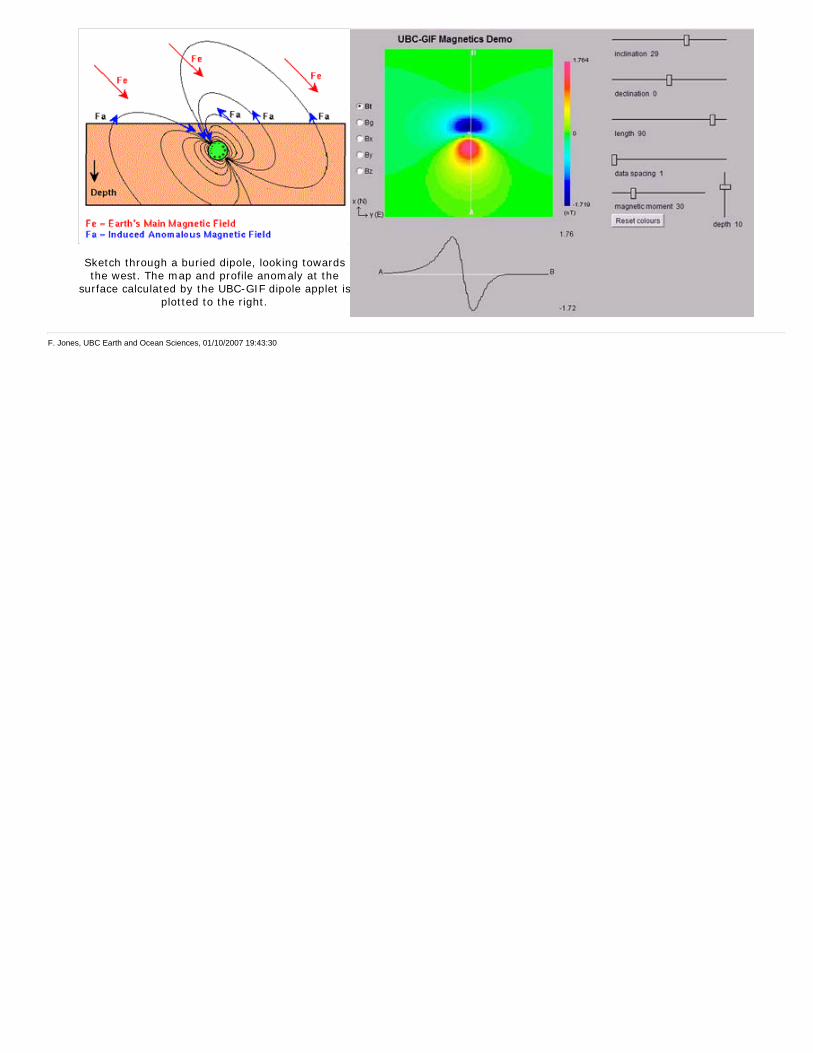
Sketch through a buried dipole, looking towards the west. The map and profile anomaly at the

surface calculated by the UBC-GIF dipole applet is plotted to the right.


Fields from extended bodies

Approximating targets as dipoles

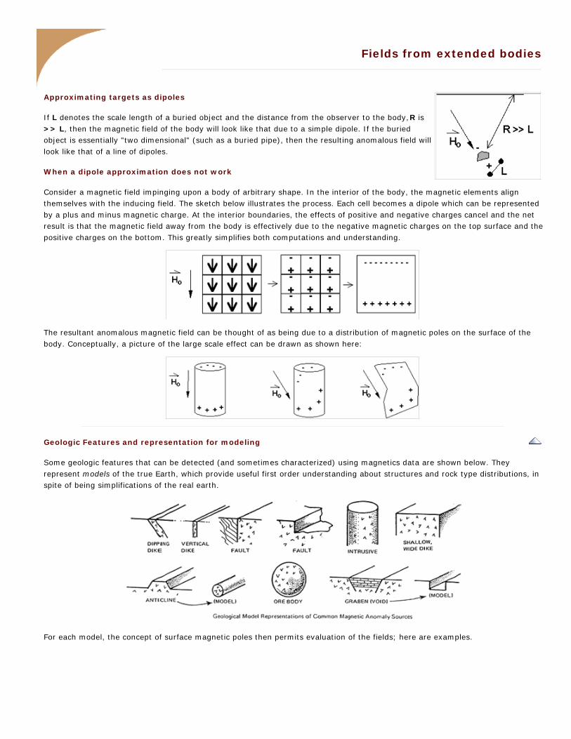
If L denotes the scale length of a buried object and the distance from the observer to the body, R is >> L, then the magnetic field of the body will look like that due to a simple dipole. If the buriedobject is essentially "two dimensional" (such as a buried pipe), then the resulting anomalous field willlook like that of a line of dipoles.

When a dipole approximation does not work

Consider a magnetic field impinging upon a body of arbitrary shape. In the interior of the body, the magnetic elements alignthemselves with the inducing field. The sketch below illustrates the process. Each cell becomes a dipole which can be representedby a plus and minus magnetic charge. At the interior boundaries, the effects of positive and negative charges cancel and the netresult is that the magnetic field away from the body is effectively due to the negative magnetic charges on the top surface and thepositive charges on the bottom. This greatly simplifies both computations and understanding.

The resultant anomalous magnetic field can be thought of as being due to a distribution of magnetic poles on the surface of thebody. Conceptually, a picture of the large scale effect can be drawn as shown here:

Geologic Features and representation for modeling

Some geologic features that can be detected (and sometimes characterized) using magnetics data are shown below. Theyrepresent models of the true Earth, which provide useful first order understanding about structures and rock type distributions, inspite of being simplifications of the real earth.

For each model, the concept of surface magnetic poles then permits evaluation of the fields; here are examples.

For these types of features, the magnetic anomalies measured along lines crossing perpendicular to them (or over their centres)usually can be directly interpreted in terms of the feature's geometry. In addition, sophisticated techniques for estimating modelsbased upon survey data can be used when more quantitative information is needed. These and other aspects of interpretation arebeyond the scope of this discussion on the basics of magnetics.

Images on this page adapted from "Applications manual for portable magnetometers" by S. BREINER, 1999, Geometrics 2190Fortune Drive San Jose, California 95131 U.S.A.


Line profiles for a range of situations

Recall that the anomaly pattern recorded over any given target depends upon latitude, targetorientation, profile orientation, remanent magnetization of the target, and possible superpositionof adjacent targets. To illustrate, here we show the anomaly recorded over two dykes buried atdifferent depths. The dykes are assumed to extend to very great distances into and out of thepage (they are 2D targets), and north is to the right (you are looking west), except in figure 3.The sketch to the right illustrates the situtation. The figures below show how data over thesedykes will depend on latitude, line orientation, target orientation, and so on. On the graph of theline profile data, note the changes in vertical scale as well as the changes in shape of the graph.

1.At mid-northern latitudes (45o) the assymetric anomaly has the low end pointing north.Buried dykes are oriented east-west.

2.At mid-southern latitudes (45o) the anomalous "low" is on the south side.

3. If buried dykes point north-south so that the survey line runs east-west, the anomalyrecorded is very different.

4.At the magnetic poles, anomalies are symmetric. (Note values for inclination and strike.)

5. At the magnetic equator, anomalies are also symmetric, but opposite those at themagnetic poles.

6. If you survey along a line that is at 45o to (rather than perpendicular) the buried 2Dtarget, the anomaly is again very different.

7. If the shallower body included some remanent magnetization, the anomaly would nowconsist of the sum of induced and remanent magnetic fields. Compare to example 2., the "normal" anomaly in the southern hemisphere.

Model earth has two 2D dykes both with susceptiblity k = 15 x 103.


Comparing data over simple and complex structures

We learned above what the anomalous magnetic field will be over a buried dipole and over extended bodies of uniformsusceptibility, and how those ideas apply to geologic structures (again, assuming uniform susceptibility). How then do we anticipate the fields due to more general geologic models of the earth? In "geophysical" terminology, the question is "how do we forward model the response to an arbitrary distribution of susceptibility?" Here is one approach that has become popular; there are 3 steps:

Describe the subsurface as a finite collection of cells, each with uniform susceptibility.1.Recognize that the response to a single rectangular cell with constant susceptibility in an arbitrary magnetizing field can be calculated relatively easily using expressions from the literature.

2.

At each location where a measurement is made above our model of the earth, the responses from all the individual cells must be added up. The result will be the superposition of all those little responses.

3.

The concept is illustrated in the following eight figures selected with the buttons. (Such calculations are introduced in section 10 and details are given in section 11. )

1. First "discretize" the subsurface under the area in which we are interested.

2. One cell of susceptible material in the cellular subsurface

4. Five susceptible cells in the descretized earth

3. Resulting magnetic anomaly at 50o magnetic north.

5. Resulting magnetic anomaly at 50o magnetic north.

6. The same data set. Not knowing what caused the anomaly, could you tell where susceptibile blocks are, and how susceptible they are?

7. A complicated earth with all cells susceptible to some degree.

8. Resulting data over the complicated earth at 50o

magnetic north.

Here again are the data generated from the single block, the 5 blocks and the continuous Earth models:

1. Total field magnetic anomaly over a single block with susceptibility of 0.1 SI units (corresponds to point 2 in the previous figure).

2. Total field magnetic anomaly over five blocks with varying susceptibility (corresponds to point 6 in the previous figure).

3. Total field magnetic anomaly over a volume with all cells having some finite susceptibility (corresponds to point 8 in the previous figure).

The following table gives access to model, mesh and data files associated with these 3 models (uniform earth, 1 block, 5 blocks) for use with UBC-GIF modelling and inversion code MAG3D. The MeshTools3D program is used to view 3D models. The filename extensions will be understandable to those familiar with use of these codes. See MAG3D in IAG's Chapter 10, "Sftwr & manuals" .

Model model file location file mesh file data file

Single block: block.sus block.sus_loc block.msh block.mag

Five block: block-5.sus block-5.sus_loc block.msh block-5.mag

Continuous earth: v.sus - v.msh v.mag


Plotting, regional trends and processing

This page is an introduction to many of the subjects related to presenting large magnetic fielddata sets. Raw data are not usually presented directly. Choices of contour plotting parametersmust be made; features not related to targets might be removed; and data or imageenhancement processing might be employed. Here we introduce some aspects of these topics.

The most common form of magnetic survey data involves "total field" measurements. Thismeans that the field's magnitude along the direction of the earth's field is measured at everylocation. To the right is a total field strength map for the whole world (a full size version is in the

sidebar mentioned in the Earth's field section).

At the scale of most exploration or engineering surveys, a map of total field data gathered over ground with no buried susceptiblematerial would appear flat. However, if there are rocks or objects that are magnetic (susceptible) then the secondary magneticfield induced within those features will be superimposed upon the Earth's own field. The result would be a change in total fieldstrength that can be plotted as a map. A small scale example is given here:

Total field strength is measured along six lines covering an area of 15 x 50 metres. With no susceptible materialunderground, all values would be the same (about 56,000 nT near Vancouver, BC.)

Values recorded will vary if susceptible material exists. These variations in total field strength can be displayed as a contourplot.

Filling the contour plot helps visualize the magnetic field variations.

Colour contour maps are now the preferred form of plotting raw "total field intensity" data.

Data along one line is often plotted as a graph in order to display more details (click here ).A more complete summary of the data set shown here is provided on a single 11" x 17" sheet in PDF format.

Large data sets are commonly gathered using airborne instruments. They may involve 105 to

106 data points to show magnetic variations over many square kilometres. An example of alarge airborne data set is shown to the right, with a larger version, including alternative colourscale schemes, shown in a sidebar.

Such data sets will be too large to invert directly, but they can provide extremely valuableinformation about geology and structure, especially if some processing is applied to enhancedesirable features and/or suppress noise or unwanted features.

Removal of regional trends

In order to interpret the magnetic data in terms of magnetic features and structures at depth, the anomalous field caused byburied features of interest must be isolated. In other words, we must try to remove the contribution to measurements consistingof the earth's field combined with fields due to geologic features larger than the actual survey area. This is accomplished byestimating and subtracting the regional, or large scale field. If we designate magnetic fields as B, then

Banomalous = Bmeasured - Bregional .

Estimates of the regional field may be obtained from:

the IGRF (International Geomagnetic Reference Field) discussed in the next section;a constant value selected by the interpreter (when survey areas are small);a more sophisticated polynomial (map) generated by a computer using least squares (or other) analysis of data;

it is also possible to use inversion at a large scale to define a regional field.

To illustrate the process, when data are collected along a line, the removal of a regional trend can be managed graphically, asshown here:

For magnetic maps (data collected over an area) the choice of a regional trend may not be particularly easy, but it is critical to getit right if a correct interpretation of subsurface distribution of susceptibility is to be obtained. Here is an example showing theregional magnetic map and a local anomalous field taken from a survey in central British Columbia.

Regional field.Airborne magnetic data gathered over a 25 square km area around a mineraldeposit in central British Columbia. Some geological structural information isshown as black lines. The monzonite stock in the centre of the boxed region isa magnetic body, but this is not very clear in the data before removing theregional trend.

Local anomalous field.Anomalous total magnetic field strength in the boxed area of the large-scalemap, after the regional SW-to-NE trend has been removed. Now thesignature of the monzonite stock is more clearly visible.

Processing options

There are numerous options for processing potential fields data in general, and magnetics dataspecifically. One example (figure shown here) is provided in a sidebar. The processing was applied

in this case in order to emphasize geologic structural trends.

Some other good reasons for applying potential fields data processing techniques are listed as follows:

Upward continuation is commonly used to remove the effects of very nearby (or shallow)susceptible material.Second vertical derivative of total field anomaly is sometimes used to emphasize the edges ofanomalous zones. Reduction to the pole rotates the data set so that it appears as if the geology existed at the north magnetic pole. Thisremoves the asymmetry associated with mid-latitude anomalies.Calculating the pseudo-gravity anomaly converts the magnetic data into a form that would appear if buried sources weresimply density anomalies rather than dipolar sources.Horizontal gradient of pseudo-gravity anomaly: gravity anomaly inflection points (horizontal gradient peaks) align withvertical body boundaries; therefore, mapping peaks of horizontal gradient of pseudo-gravity can help map geologiccontacts.

The effects of these five processing options are illustrated in a separate sidebar on processing of magnetics data.


Background - Earth's field

Introduction

All geophysical surveys involve energizing the earth and measuring signals which result from the earth's effect upon that energy. Measurements will contain information about the types and distributions of subsurface physical properties.

In the introductory section, it was noted that magnetic surveys involve measuring fields that are induced in magnetically susceptible materials by Earth's magnetic field. On this page, we provide some essential background about the static and dynamic characteristics of this natural field.

Source: Earth's field

Most people are familiar with the magnetic field that exists around a dipolar or "bar" magnet (shown to the right as the pattern of iron filings on paper over a bar magnet). To a first approximation, Earth's magneticfield looks like that of a dipolar source within the Earth, which is tilted about 11.5 degrees from the spin axis and is slightly off centre. This field has a strength of approximately 70,000 nanoTeslas (nT) at the magnetic poles and approximately 25,000 nT at the magnetic equator. Units for magnetics work are discussed in the separate chapter on units. The figure below-left illustrates a cross-section of the field as it could be imagined from space. Below-right is a sketch of the directions of the field at Earth's surface.

There are, in fact, three different components to Earth's field:

The main dipolar field of the earth (produced internally by large currents in the fluid outer core of the earth).1.External variations caused by currents flowing in the ionosphere. For magnetic surveys, this is a source of "noise", and is the reason the field in the left-hand image above appears asymmetric.

2.

Magnetic fields due to rocks or buried bodies that are the objective of geophysical surveys. These fields are the "signals" we have to work with, and they may be either permanent (always present, regardless of the ambient local field) or induced (caused by Earth's field).

3.

Describing Earth's field

The convention for describing Earth's field is to have a negative pole in the northern hemisphere and a positive pole in the southern hemisphere. Therefore, the magnetic field on Earth's surface looks approximately like that given in the right-hand figure above. Using B to represent the magnetic field of Earth as a vector in three dimensions, the field at any location on (or above or within) Earth can be described in either of three ways (refer to the next figure below):

B = (Bx, By, Bz) = (X, Y, Z) in the figure. These are cartesian coordinates with X pointing to true (geographic) north, Ypointing east and Z pointing vertically down.B = (Bh , Bz , D) = (H, Z, D) in the figure. These are horizontal and vertical components, plus declination (angle with respect to true north).B = (D, I, |B| ). These are the commonly used polar coordinates which include two angles and a magnetude: D=declination, I=inclination, and |B|=total field strength.

In 2004, Earth's north magnetic pole was close to Melville Island at (Latitude, Longitude)=(79N, 70W). At Vancouver D ~ 20o

east, I ~ 70o down from horizontal.

Sketch of coordinates used to describe magnetic fields.

B is the vector representing magnetic field of the earth.B represents its magnitude of field strength (sometimes referred to as F).H is the projection of the field, B, onto the surface.Z is the projection of the field, B, onto the vertical direction.X is the projection of the field, B, onto the northward direction.Y is the projection of the field, B, onto the easatward direction. D: declination is the angle that H makes with respect to geographic north.I: inclination is the angle between B and the horizontal. It can vary between-90° and +90°.

The details of Earth's field at any location on Earth are described using a formula based upon a spherical harmonic decomposition of the field called the IGRF or International Geomagnetic Reference Field. Details about Earth's field can be found at government geoscience websites (listed below) such as the NOAA Geomagnetism home page, or the Canadian National Geomagnetism Program's home page. Resources about Earth's global magnetic field are:

A sidebar describing the International Geomagnetic Reference Field.

Three figures show how declination, inclination and field strength varies around the world.

NOAA Geomagnetism home page, and the Canadian National Geomagnetism Program's home page websites. Find parameters describing Earth's field at a specific location (specified using date, latitude, longitude and elevation) at the NOAA National Geophysical Data Center's online magnetic field calculator.

Variability of Earth's field

The source of the main (nearly dipolar) field varies slowly, causing changes in strength, declination and inclination over time scales of months to years. Changes in the exact location of the magnetic north pole are caused by this effect. See the Geological Survey of Canada's website for a conversational history of the location of the Magnetic North pole. Declination varies very widely in Canada. The correct value of declination can be found by entering your latitude, longitude and year at the GSC's website.

The second component of Earth's field involves external contributions due primarily to currents in the ionized upper atmosphere.

Daily variations (on the order of 20 - 50 nT in size) are due to solar wind action on the ionosphere and magnetosphere. The image shows an artist's rendition of the charged particles interacting with Earth's magnetic field. An overview of Earth's magnetic field(with good images, graphs, etc.) can be found on the British Geological Survey's geomagnetics web site.Magnetic storms are correlated with sunspot activity, usually on an 11-year cycle. These variations can be large enough to cause damage to satellites and north-south oriented power distribution systems. They are also the cause of the Aurora Borealis or Australis(northern or southern lights respectively). See the GSC's "Geomagnetic Hazards" web page for more.

Temporal variations are often larger than geophysical anomalies. They must be accounted for in all surveys. The only exception is gradient magnetic surveys gathered using two sensors. Three figures are given in a sidebar showing examples of different

types of magnetic noise that may be encountered at time scales of several days, hours, and minutes.

The Geological Survey of Canada has a web page, which can provide graphs of diurnal variations observed at any of 11 magnetic observatories in Canada, for any day in the most recent 3 years. Find this facility by starting at the GSC Geomagnetic data page.


Physical principles underlying magnetics

On this page:| Origin of magnetic fields| Magnetic induction, and relating B & H

| Magnetic pole strength | The anomalous field

Origin of magnetic fields

All magnetic fields can be thought of as arising from electric currents. We are all familiar with the experiment inwhich a compass is held close to a wire, which can be attached to a battery. The compass needle is deflectedwhen the current flows in the circuit. The compass itself consists of a magnet that is free to rotate. The fact thatit moves indicates that the current produces a magnetic field. This was found by H. C. Oersted in 1820, and the

Biot-Savart law quantifies the effect: magnetic field strength, , at a distance, r, from a straight wire carrying current, I, in Amperes is given by the mathematical expression

(1)

The magnetic field, , is a vector. In the case of the line current, it points in a direction around the wire, given by the right

hand rule. This is indicated by the unit vector, . The units of are Am-1 (Amperes per meter).

Magnetic field of a circular loop

If the current-carrying wire is bent into a loop, it produces a magnetic field with the geometry shownhere. As with a straight wire, the direction of the magnetic field is given by the right hand rule. The fieldhas the same configuration as that of a small "bar magnet" placed perpendicular to the loop's plane, atits centre. The strength of this magnetic, called m, the magnetic moment, is proportional to the

current and the loop's area, A. So m=IA=I r2 and has units of Am2. If the radius of the loop is a and if you observe from a distance, r, much greater than this radius (r >> a), then the strength of the field,

H, decreases as 1/r3. This is a much greater rate of decrease than the 1/r we had for a long straight wire (above).

All magnetic fields are caused by currents (moving electric charges)

We can use the relation between current loops and magnetic fields to account for anymagnetic field. Consider a single atom made of protons, neutrons and electrons. Protons andelectrons are charged particles which can rotate on their axes, and electrons revolve aroundthe nucleus. One can think of these motions as "circular currents" and each circular currentproduces its own magnetic field. Some of the magnetic fields may cancel. For instance,electrons can have a spin up or down, but it is possible for an atom to have a net magneticmoment. This occurs especially for those atoms that have unpaired spins of the electrons. For magnetic materials, all of themagnetization that we see will be related to the cumulative effects of the magnetic moments of all of the individual atoms. In fact,the orbital motion of electrons gives rise to the diamagnetic component, and the spin motion of electrons gives rise to paramagnetic effects.

Magnetic charge and dipoles

Despite the fact that all magnetic fields have their origin in moving electric charges, it is convenient to introduce a magnetic"charge," Q, which has dimensions of Wb (Weber). Other words for Q are magnetic monopole, or pole strength. The force between two magnetic charges Qa and Qb is given by

(2)

This is very similar to Coulomb's law, which gives the electrostatic force between to electriccharges. We note that our magnetic force, F, is repulsive when the magnetic charges are the same sign ("like" poles repel) and the force is attractive when the charges have opposite sign("unlike" poles attract). The magnetic field measurable at the location of one of the charges is

the force on that charge divided by its strength,

(3)

In fact, the magnetic field strength, , can be thought of as the magnetic analog to the gravitational acceleration, g.

Magnetic fields of a dipole

Consider two magnetic charges of opposite magnitude (Qa = P, Qb = -P) and separated by a distance of l in free space. We refer to this configuration as a dipole. The strength of this dipolar magnet, or its magnetic moment is given by

(4)

The magnetic field away from the dipole is the superposition of the fields from the individualpoles. Applying expression (3) above for the field due to both poles, we have

(5)

If r >> l then the magnetic field, , some distance away from a dipole can be found using

some simple geometry. Using the polar coordiantes defined in the figure, is given by

(6)

In fact, this expression turns out to be precisely the same as that due to a circular loop currentthat has the same magnetic moment, but where m = IA. The similarity of fields due to a circular current loop and a magnetic dipole is emphasized in the next figure.

This correspondence has extremely important implications because it means we can think of materials as being made up of smallmagnets. We have substantial intuition about how small magnets act in the presence of larger magnets (everyone has put a largemagnet under a sheet of paper containing iron filings). With this background, we obtain fundamental intuition about magneticexperiments. The four figures below illustrate further.

Forces associated with magnetic monopoles

Forces associated with magnetic dipoles

Fields due to the individual negative (yellow) and positive (blue) poles combine using vector addition into a total field shown in

The net field due to a dipolar source.

(purple) here, and separately to the right.

Magnetic pole strength (surface density of magnetic charge)

The anomalous magnetic field resulting from an irregularly shaped object can be accounted for using an equivalent distribution ofmagnetic poles on the surface of the object. Intuitive pictures can be drawn by aligning the interior magnets in the direction of theinducing field.

If the magnets point across a surface of the body, then there will be an effective pole density there. If the magnets point parallelto the interface, then the pole density will be zero.

The above not only helps with conceptualizing the character of the magnetic field, but also provides a way to calculate it directly.The magnetic field measured a distance, r, from a pole of unit strength is

(8)

where is a unit vector pointing from the elementary pole to the observer. To find the field of the magnetized object we sum

(integrate) the contributions arising from all of the poles on the surface of the body. Using the fact that is the induced

magnetization per unit volume (that is, = K o ), the final field is

(9)

where is the outward-pointing normal vector to the surface.

The anomalous field

In applied geophysics, it is common to refer to measurements as "the magnetic anomaly." This can be defined as the observedmagnetic value minus a background or reference value, usually dominated by the inducing (Earth's) field. What will thisanomalous field look like when total field measurements (such as those taken with a proton precession or optically pumpedmagnetometer) are recorded? To find out, we must analyse the combination of measurement in terms of the vector componentsof all contributing fields.

Let the earth's magnetic field (really, magnetic flux) be denoted by o (vertical in the figure

here). Let the field from the buried magnetic feature be denoted by a. The field measured atthe surface of the earth is the sum of the earth's field and the field from the buried feature. Theanomalous component of that total field may be directed up or down depending upon whatportion of the anomalous field is being observed (see positions A and C in the diagram).

The anomalous magnetic field that we want from a proton precession magnetometer (to be called

B) is the measured field amplitude minus the amplitude of the earth's field (which can also be called the inducing or primary field):

(10)

B can usually be written in an approximate form. Let o be a unit vector in the direction of the inducing field. In most cases |

o| >> | a|. The situation can be illustrated using the following vector diagram:

The angle θ is the angle between the Earth's magnetic field and the anomalous magnetic field. Simple trigonometry tells us that

(11)

Equivalently, we can use the vector dot product to show that the anomalous field is aproximately equal to the projection of thatfield onto the direction of the inducing field. Using this approach we would write

(12)

This is important because, with a total field magnetometer (like a proton precession or optically pumped sensor), we can measureonly that part of the anomalous field which is in the direction of the earth's main field.

Whether we work with vector component magnetometers (such as fluxgate instruments) or total field magnetometers, we areeffectively able to measure only a component of the anomalous magnetic field. Here is one way to think about the measurement:

A fluxgate oriented horizontally in the direction measures Bax, the projection of the anomalous field in the x-direction.1.A fluxgate oriented vertically in the direction measures Baz, the projection of the anomalous field in the z-direction.2.A total field magnetometer measures the total field. When we subtract the magnetic field of the earth to get the anomaly,then we obtain the projection of the anomalous field onto the direction of the earth's magnetic field at that location.

3.

Measured quantities are given by:

Magnetic anomaly example

So if we know the anomalous magnetic field that arises from any magneticbody, then we also can determine what the instrument will measure. It will bethe projection of the anomalous field onto the inducing field's direction. Anexample of the result is shown in these final three figures. Red arrows showEarth's field's direction, blue arrows show induced field vectors, and the sign ofmeasurements can be determined by comparing the directions of these twofields at each location on the earth's surface.

On a piece of paper, sketch a blank version of the empty graph; then try tosketch qualitatively the measurement you would expect along the surface. Forexample, at the equator (Figure 1) the largest measurement will be above thecentre of the buried object, and it will have negative magnitude because theobject's field points in the opposite direction to the earth's field. Confirm yoursketches using the "Solution" buttons.

1. - Total field magnetic anomaly over a buried dipole at the magnetic

equator. (Solution )

2. - Total field anomaly at the magnetic north pole. (Solution )

3. - Total field anomaly at magnetic mid latitudes. (Solution )


Magnetic induction and magnetic units

There is often confusion regarding units in magnetics. This arises because relations can be derived from either of two fundamental

principles, and the results yield different units. In the cgs and emu system of units, is derived from the concept of magnetic

force due to magnetic poles. The magnetizing field (or magnetic field strength), , is defined as a force on a unit pole, so it hasunits of dynes per unit pole, which are called oersteds. In the SI system of units, magnetic field is defined in terms of the

consequence of current flowing in a loop. Then, has units of amperes per meters (which = 4 × 10-3 oersted).

Now, what if there is a magnetizable body in the presence of ? The body becomes magnetized due to the reorientation of atomsand molecules so that their spins line up. The amount of magnetization, m, is quantified as magnetic polarization, also known as magnetization intensity or dipole moment per unit volume. The lineup of internal dipoles produces a field, m, which, within the

body, is added to the magnetizing field. m has units of ampere-meter2 per meter3, which is amperes per metre, the same as .

In low magnetic fields, m is proportional to ; in fact, m = k , where k is magnetic susceptibility, a physical property. k in the two systems of units is related according to kSI=4 kemu.

The magnetic induction (or magnetic flux density), , is the total field within the magnetic material, including the effect of

magnetization. can be written as:

= µo( + m) = (1 + k)µo = µrµo .

The SI unit for is the tesla, which is 1 newton/ampere-meter. The cgs-emu unit for is the gauss, which equals 10-4 tesla. The

magnetic permeability of free space (considered a universal constant) is µo = 4 × 10-7 H/m (the units are Henries/meter). The parameter µr is the relative magnetic permeability, and its value is essentially 1 in air or free space. The permeability, µ, is sometimes used, and it is the quantity (1 + k)µo = µrµo = µ.

The above relation shows how a material's magnetic permeability relates to its magnetic susceptibility, k , and how the magneticflux density within a material depends upon both the ambient field and the induced magnetic moment. There can be someconfusion as to whether permeability, µ, or the relative permeability, µr, is being used, but you should be able to tell by the value.However, it is best to check, if possible. Susceptibility is becoming the most commonly used physical property for geophysicalwork, but use of permeability can still be found in older work, or in some countries.

The tesla is a large unit compared to the magnetic fluxes that we ordinarily deal with in applied geophysics, so we generally use a

subunit nanotesla (nT) where 1 nT=10-9 T. There is also another unit, the gamma, which is numerically equivalent to the nT. That is, 1 nT = 1 gamma. The strength of the earth's magnetic field varies between approximately 25,000 and 70,000 nT, dependingupon latitude.

So, in the end, are we measuring or during geophysical surveys? This confusion stems partly from the fact that the two arelinearly related, so that a map of one looks exactly like a map of the other, except for the units. Most geophysical magnetic

surveys involve measuring and maps are shown in units of nanoteslas. If the maps and interpretations are discussed in terms of

, the conclusions will not change, so the distinction is not usually worried about.

See also the sidebar on magnetic units, which discusses units in the context of the UBC-GIF dipole JAVA applet., which in

turn, is discussed more fully in the section which discusses the response to buried dipoles .


Introduction to forward modeling

"Forward modelling" means calculating the data when subsurface structure, and the physics of the problem, are both well known.Two approaches are common. The first involves calculating the magnetic effect at every measurement location due to a buriedpolygonal structure of uniform susceptibility (or several such polygons). The method is based upon fundamental properties ofdipolar potential fields and is not discussed further in this module. The second involves calculating the effect at locations due to a"digitized" Earth. This is a more general approach, but is challenging because working with fully generalized Earth models canresult in a large number of calculations. For example:

If the earth is divided up by specifying 100 x 100 x 50 cells (defining, for example, a 1 km square region 500 m deep, using10 m cubic cells), then there will be M=100x100x50=500,000 cells.Now, if you want to simulate the recording of data along survey lines 50 m apart with measurements at 10 m spacings,then you have 21 lines x 101 stations = N = 2,121 data points. To calculate the magnetic field at all these points, due to all the cells, you end up with a total of MxN=1.06x109 (1.06billion) calculations!

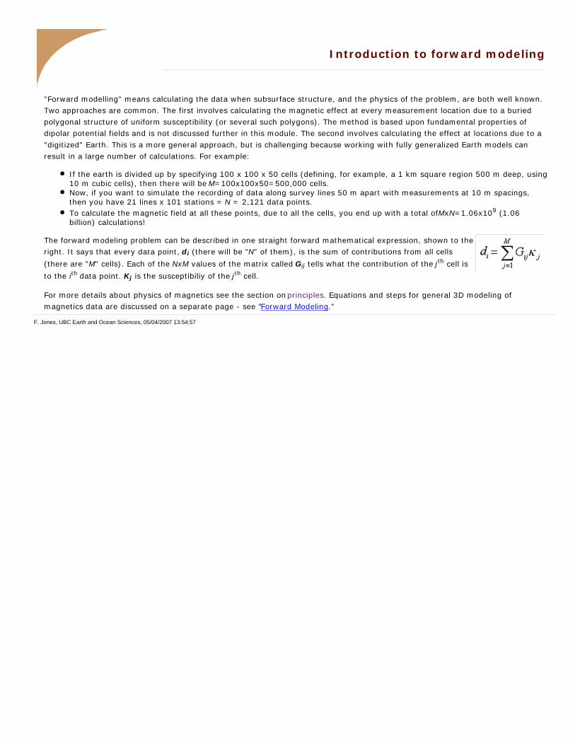
The forward modeling problem can be described in one straight forward mathematical expression, shown to theright. It says that every data point, di (there will be "N" of them), is the sum of contributions from all cells

(there are "M" cells). Each of the NxM values of the matrix called Gij tells what the contribution of the jth cell is

to the ith data point. Kj is the susceptibiliy of the jth cell.

For more details about physics of magnetics see the section on principles. Equations and steps for general 3D modeling ofmagnetics data are discussed on a separate page - see "Forward Modeling."


Forward modeling: calculating magnetic data

On this page: | Goals | Scalar potential (the dipole) | Many dipoles (a volume of susceptible material)

| The discrete version and Green's tensor formulation | Forward vs Inverse problems

Goals

We want to calculate observations of B (magnetic flux density) at any location in three dimensions, for an arbitray 3D distribution of susceptible material, with any orientation of inducing field. This is a general case of the magnetics forward modelling problem. Specific cases that will not be discussed here include calculating fields everywhere due to a solid polygon of susceptible material, and calculating fields of other more constrained geometries. For our more general situation, known parameters will be (1) susceptibility within each cell of a discretized volume of earth, and (2) the geometry of the datum location with respect to each cell. Conceptually, the earth under the surface will be divided into discrete cells, as illustrated in the sketch to the right showing an airborne magnetic survey.

To solve the forward problem for magnetics, two fundamental relations are needed: (i) one of maxwell's equations, and (ii) a relation for the magnetic field due to a dipole expressed in terms of a scalar potential. On this page, the solution will be outlined only. Details of the various steps can be found in texts and references that discuss the theory of potential fields theory and applied geophysics. Some suitable texts are listed a separate references page.

Scalar potential

We start with Maxwell's equation relating magnetic field to current (based upon Ampere's law):

(1).

This equation states that the curl of magnetic field is equal to the vector sum of all moving charges within the region. The Jf is free current density, the second term involves currents related to internal magnetic fields, and the last term accounts for displacement currents.

For geophysical situations we can assume there are no significant currents within the region of interest. Therefore the right hand side goes to zero. Consequently, B is an irrotational field so, according to the Helmoltz theorem, there must be a scalar potential V such that

(2) .

Scalar potential due to a magnetic dipole

Next we need an expression for magnetic potential at some distance from a small magnetic dipole. Formulate this in terms of scalar potential V(q) at point q some distance from the dipole:

(3).

The magnetic dipole itself can be expressed in either of two ways.

As an elemental current loop, as shown. Q is the observation location, I is the current in the loop and the m is dipole moment, which is I x surface area, in the direction perpendicular to the loop according to the right hand rule. The rhat is a unit vector in the direction from dipole location towards observation point.

1.

In terms of a pair of equal but opposite monopoles, the dipole moment is p x ds where p is the monopole strength and ds is the vector distance between them.

2.

More details about this topic, refer to Blakely, pg 72.

B for arbitrary volumes of susceptiblity

The magnetic field due to a volume full of dipoles is found by integrating the single dipole expression:

(4) .

Now take the gradient of this scalar potential to find B due to a volume of dipoles:

(5) .

The gradient comes inside since both integration and gradient operators are linear and therefore commutative.

Now we want the magnetic field at any position ri . This is given as a function of a distribution of dipoles, m(r), which in turn is a

function of the distribution of susceptibility and inducing field because (6):

(7)

Evidently the magnetic field calculations depend upon

the ambient field strength and direction, the distribution of susceptible material below the surface, and the position of the measurement.

Recall that the ambient field is described in terms of strength, inclination and declination, as shown in the figure to the right.

The discrete version

First assume . Also ignore remanent magnetization and self-magnetization. This is valid for most

geologic materials because their susceptibility is not very large, but it is not always true. Then discretize the earth into M cells, each with constant k. Now each datum, Bi, will include contributions from all j = 1… M cells:

(8)

Regarding rectangular discretization, a general earth structure can be adequately modelled if this type of discretization is fine enough. However the problem becomes large very quickly if too many cells are used. For realistic mineral exploration surveys cells that are 25 x 25 x 12.5 metres are usually adequate, although much larger cells are necessary if the survey area is large.

Green's Tensor formulation

We can now conclude by using what we have covered so far on this page to identify the Green’s Tensor formulation for forwardmodelling:

Each datum bi is a component of the anomalous (induced) B along some direction - for total field measurements this is the direction of the incident field:

(9)

Pose the problem in terms of susceptibilities using (8);

(10)

where the Gij are calculated by

(11)

in which T is called the "Green's tensor". Equation (10) is what we were looking for, namely a forward modelling equation which can calculate measurements anywhere in space caused by a general distribution of susceptible material which is within an ambient (inducing) field with any strength and direction.

Forward vs Inverse problems

Now we can describe the two fundamental geophysical problem types using these equations.

Forward calculations involve: Given a susceptibility distribution kj = 1, ..., M, and a well-described ambient field, calculate the data bi=1, ..., N.

or, in matrix form, (12) .

Inversion involves: Given the data bi , i=1, ..., N, some understanding of their reliability, and a well described ambient field, estimate the susceptibilities kj , j = 1, ..., M such that

(13).

This page is not the place to discuss inversion, but this illustration should provide an initial perspective on how the forward calculations (finding data knowing models) and inversion problems (finding models knowing data and errors) are related.


Instruments for magnetic surveys

Instruments

A measurement of the magnetic field at any location will involve either recording the magnitude in one or more vectorialcoordinate directions, or a magnitude in the field's direction (commonly referred to as "total field strength"). There are manymanufacturers of magnetometers for ground, marine, helicopter, fixed wing, and space-borne geophysical use. Instrument typescommonly used are outlined very briefly as follows:

Fluxgate Magnetometer

This type of instrument was developed during WWII to detect submarines. It measures the magnitude in a specific directiondetermined by the sensor's orientation. A complete measurement of the field requires three individual (cartesian)components of the field ( such as Bx, By, Bz).It is generally difficult to get leveling and alignment accurate. Sensor accuracy is 1 nT so orientation must be known towithin .001 degrees.There are some fluxgates which generate a measure of the total field strength.

Proton Precession Magnetometer

This instrument was the most common type before the mid 1990's. It measures the total field strength.Advantages: Sensitive to 1 nT, small, rugged & reliable, not sensitive to orientation. Disadvantages: Takes >1 sec to read, sensitive to high gradients. The measurement process is related to nuclear magnetic resonance (NMR). A proton source (possibly as simple as a volume of water) is subjected to an artificial magnetic field, causing the protons to align with the new field.When the artificial field is removed, the protons precess back to their original orientation and their precessionfrequency (called the Larmor precession frequency) is measured. That frequency, f, is related directly to thestrength of the earth's field according to the equation to the right. The parameter, p, is the ratio of the

magnetic moment to spin angular momentum. It is called the gyromagnetic ratio of a proton and is known to 0.001%; p

= 2.67520 x 108 T-1s-1.

Cesium (or optically pumped) magnetometer:

The physics behind this type of sensor is related to that of the proton precession sensor, but it is more complicated.Although it is more expensive than the above two sensor types, it is now the most commonly used system for small scalework because it is 10 to 100 times more sensitive than the proton precession magnetometer.The measurement process makes use of the gyromagnetic ratio of electrons and of the quantum behavior of outer-shellelectrons of some elements (e.g. cesium). In this case, the relevant gyromagnetic ratio is known to 1 part in 107 , and frequencies are near 233 khz, so these instruments are sensitive to 0.01 nT. Advantages: More rapid readings, 1 or 2 orders of magnitude more sensitive, works in high gradients. Disadvantages: Optical pumping won't work when parallel or perpendicular to mag field direction (solved with multiplesensors), more expensive than proton precession.

SQUIDS (superconducting quantum interference devices): These are very sensitive, and are currently more common inlaboratories that work on rock magnetism or paleomagnetic studies. However, they are beginning to be used in the field, andmore applications will become evident in the coming decade (2000 - 2010). Search the internet using, for example, "squid ANDmagnetometer AND geophysics" as keywords.

Magnetic Gradiometer

These instruments use two sensors (any of those mentioned above) to measure vertical or horizontal gradients.They often employ two cesium magnetometers separated by about 1 m.


Documents

Magnetic surveys - University of British Columbia · Magnetic surveys Geophysical magnetic surveying makes use of the fact that Earth's magnetic field causes, or induces, subsurface