278

Chapter 11

11.1 (a) The linear discriminant function given in (11-19) is

A (_ - )'8-1 AIY = Xl - X2 pooled

X = a X

where

S~moo = ( _: -: i

so the the linear discriminant function is

((: i - (: iH -: -: 1 z=¡-2 ~=-2Xi

(b)

A l(A A) l(AI AI)' 8m = - Yl + Y2 = - a Xl + a X2 =-2 2Assign x~ to '11 if

Yo = (2 7)xo ~ rñ = -8

and assign Xo to '12 otherwise.

Since (-2 O)xo = -4 is greater than rñ = -8, assign x~ to population '11-

279

11.2 (a) '11 = Riding-mower owners; 1T2 = Nonowners

Here are some summary statistics for the data in Example 11.1:

Z¡ - (I:,,::: 1 '

5, - ( ~:::::: -I::::: 1 '

_(.276.675 -7.204 i

8 pooled - ,-7.204 4.273

Z2 - 1:::: 1

82 = ( 200.705 -2.589 1-2;589 4.464

( .00378 AJ06371

8-1pooled =

.00637 .24475

The linear classification 'function for the data in Example 11.1 using (11-19)

is

( (109.475 i -( 87.400 i) i ( ,0037820.267 17.633 .00637

where

.006371 r J'x = L .100 .785 :.

.24475

1 1ri = 2"(Yl + Y2) = 2"(â'xi + â'X2) = 24.719

280

(b) Assign an observation x to '11 if

0.100x¡ +0.785xi ~ 24.72

Otherwise, assign x to '12

Here are the observations and their classifications:

Owners NonownersObservation a'xo Classification Observation a/xo Classification

1 23.44 nonowner 1 25.886 owner2 24.738 owner 2 24.608 nonowner3 26.436 owner 3 22.982 nonowner4 25.478 owner 4 23.334 nonowner5 30.2261 owner 5 25.216 owner6 29.082 owner 6 21. 736 nonowner7 27.616 owner 7 21.500 nonowner8 28.864 owner 8 24.044 nonowner9 25.600 owner 9 20.614 nonowner

10 28.628 owner 10 21.058 nonowner11 25.370 owner 11 19.090 nonowner12 26.800 owner 12 20.918 nonowner

From this, we can construct the confusion matrix:

Actualmembership :~ j

PredictedMembership'11 '1211 12 10

Total1212

(c) The apparent error rate is 1~~i2 = 0.125

(d) The assumptions are that the observations from 7íi and 7í2 are from multi-

variate normal distributions;with equal covariance matrices, Li = L2 = .L.

11.3 l,Ne ned.t-o 'Shuw that the regiuns Ri and R2 that minimize the ECM are defid

281

by the values x for which the following inequalities hold:

Ri : fi(x) ;: (C(lj2)) (P2)h(x) - c(211) Pi

R2 : fiex) ~ (cC112)) (P2)h(x) c(211) Pi

Substituting the expressions for P(211) and p(ij2) into (11-5) gives

ECM = c(211)Pi r fi(~)dx + c(li2)p2 r h(x)dxJ R2 J RiAnd since n = Ri U R2,

1 = r h(x)dx + r h(x)dx 'J Ri J R2

and thus,

ECM = c(211)Pi (1 - k.i fi(x)dx) + c(112)p2 ~i h(x)rix

Since both of the integrals above are over the same. region, we have

ECM = r (c(112)p2h(x)dx - c(21 l)pifi (x)ldx + c(2~1)PiJRi

The minimum is obtained when Ri is chosen to be the regon where the term in

brackets is less than or equal to O. So choose Ri so that

c(211)pifi( x) ;: c(112)pd2(:i )'Ur

282

h(æ) )0

(C(112) ) (P2)h(x) - c(2j1) Pi

11.4 (8) The minimum ECM rule is given by assigning an observation :i to '11 if

fi(æ) )0 (C(112)) .(pi) = (100) (~) = .5

h(x) - c(211) Pi 50.8

and assigning x to '12 if

fi(x) ~ (C(112))(!!) = .(100) (.2) = .5f2(x) c(211) Pi 50.8

(b) Since fi(x) = .3 and f2(x) = .5,

fi(x) = 6;: 5

hex) . -'

and assign x to '11'

11.5 - ~ (~-~1)'t-1(~-~1) + ~ (~-~2)lt~1(:-~2) =

1 1 1 1 - 1 1+- 1 l +-1 1- 2(~lr :-2:~r ~+~~r, :i-~'t :+2:2+ :-~2+ ~2

1 i - 1 l l- 1 1,,- 1 J= - 2(-2(:1-:2) ~ ~+~l~ :1-:2~ :2

i -1 i ( ) i l- 1 ( )= (:1-:2) t : -2 :'-:2 If :1+~2.

283

11.6 a) E(~'I~I7ii) -aa = .:!:l - m = ~l!:i - ~ ~l(~i + !!2J

= 1 ~I (~i - !!2) = ~ (!:i - !:2) i r i (~i -!!) ~ 0 s ; nee

r1 is positive definite.

b) E ( ~,1 ~ lir 2) - II = ~ 1!:2 - m = l ~l (~2 - ~1)

_ 1 ( ),..-1 (- - '2 ~l - ~2'" ~l - ~2) ~ 0 .

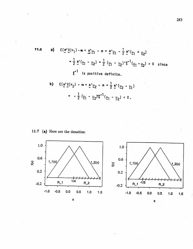
11.7 (a.) Here are the densities:

1.0 1.0

R_1 -1/3 R_2

0.6 0.6x-- ~0.2 0.2

-0.2 R_1 1/4R_2

-0.2

-1.0 -0.5 0.0 0.5 1.0 1.5 -1.0 -0.5 0.0 0.5 1.0 1.5

x x

284

(b) 'When Pi = P2 and c(112) = c(211), the classification regions are

R . hex) ~ 1i . hex) - !i(x)R2 : h (x) ~ 1

These regions are given by Ri : -1 ~ x ~ .25 and R2 : .25 ~ x ~ 1.5.

(c.) When Pi = .2, P2 = .8, and c(112) = c(211), the clasification regions are

Ri : fi(x) ;: P2 = .4hex) - Pi

fiex)R2 : h (x) ~ .4

These regions are given by Ri : -1 ~ x ~ -1/3 and R2 : -1/3 ~ x ~ 1.5.

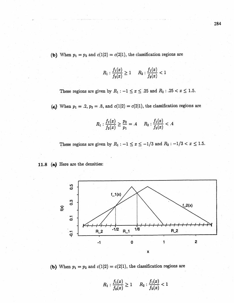
11.8 (al Here are the densities:

i.ci

C'ci-

~,.ci

,.ci

i

R_2 -1/2 R_1 1/6 R_2

-1 o 1 2

x

(b) When Pi = P2 and c(112) = c(2Il), the classification regions are

R . h(x) ;: 11 . h(x) - !i(x)R2 : hex) .( 1

11.9

285

These regions are given by

Ri : -1/2 =: x ~ 1/6 and R2 = -1.5 ~ x ~ -1/2, 1/6 ~ x ~2.5

a'B ,ua

a/La!'((~1-~)(~1-~)' + (~2-~)(~2-~),J~'=

a1ta- -

hI, + ) Thus "_1 - u-_ = l(2. ll_l - U_2) and 11_2 - ~ =w ere ~ = 2' ~1 ~2. ~

tt ~2 - ~l ) so

a'B ,ua =

a/La! ~I (~1-~2)(~1-~2) I ~

Iala- -

,

28~

11.10 (a) Hotellng's two-sample T2-statistic is

T2 - (:Vi - X2)' f (~i + n~) Spooled J -i (Xi - X2)

- (-3 - 2j ((I~ + 112) l-::: -::: If L ~: I = 14.52

Under Ho : l.i = 1J2,.. ..

T2", (ni + n2- 2)p F. . .+ 1 p,nl+n2-p-lni n2 - P -

Since T2 = 14.52 ~ ~i~i~~-;~~ F2,2o(.1) = 5.44, we reject the null hypothesis

Ho : J.i = J.2 at the Q' = 0.1 level of significance.

(b) Fisher's linear discriminant function is

Yo = â'xo = -.49Xi - .53x2

(c) Here, m, = -.25. Assign x~ to '1i if -A9xi - .53x2 + .25 ~ O. Otherwise. iassign Xo to '12.

For x~ = (0 1), Yo = -.53(1) = -.53 and Yo - m = -.28 ~ o. Thus, assign

Xo to '12.

287

11.11 Assuming equal prior probabiliti€s Pi = P2 = l, and equal misclasification costs

c(2Il) = c(112) ~ $10:

Expectedc P(BlIA2) P(B2IAl) P(A2 and Bl) peAl and B2) P( error) cost9 .006 .691 .346 .D03 .349 3.4910 .023 .500 .250 .011 .261 2.6111 .067 .309 .154 .033 .188 1.8812 .159 .159 .079 .079 .159 1.59!13 .309 .067 .033 .154 .188 1.8814 .500 .023 .011 .250 .261 2.61

Using (11- 5) ) the expected cost is minimized for c = 12 and the minimum expected

cost is $1.59.

1i.~2 Assuming equal prior probabiltiesPi = P2 = l, and misclassificationcosts c(2Il) =

$5 and c(112) = $10,

expected cost = $5P(A1 and B2) + $15P(A2 and B1).

Expectedc P(BlIA2) P(B2/A1) P(A2 and Bl) P(AI and B2) P(error) cost9 0.006 0.691 0.346 0.003 0.349 1.7810 0.023 0.500 0.250 0.011 0.261 1.4211 0.067 0.309 0.154 0.033 0.188 1.2712 0.159 0.159 0.079 0.079 0.159 1.5913 0.309 0.067 0.033 0.154 0.188 2.4814 0.500 0.023 0.011 0.250 0.261 3.81 .

Using (11- 5) , the expected cost is minimized for c = 10.90 and the minimum

expected cost is $1.27.

11.13 Assuming prior probabilties peAl) = 0.25 and P(A2) = 0.715, and misoassIÍca-

tion costs c(2Il) = $5 and c(lj2) = $10,

expecte cost = $5P~B2jAl)(.2'5) + $15P(BIIA2)(.75).

288

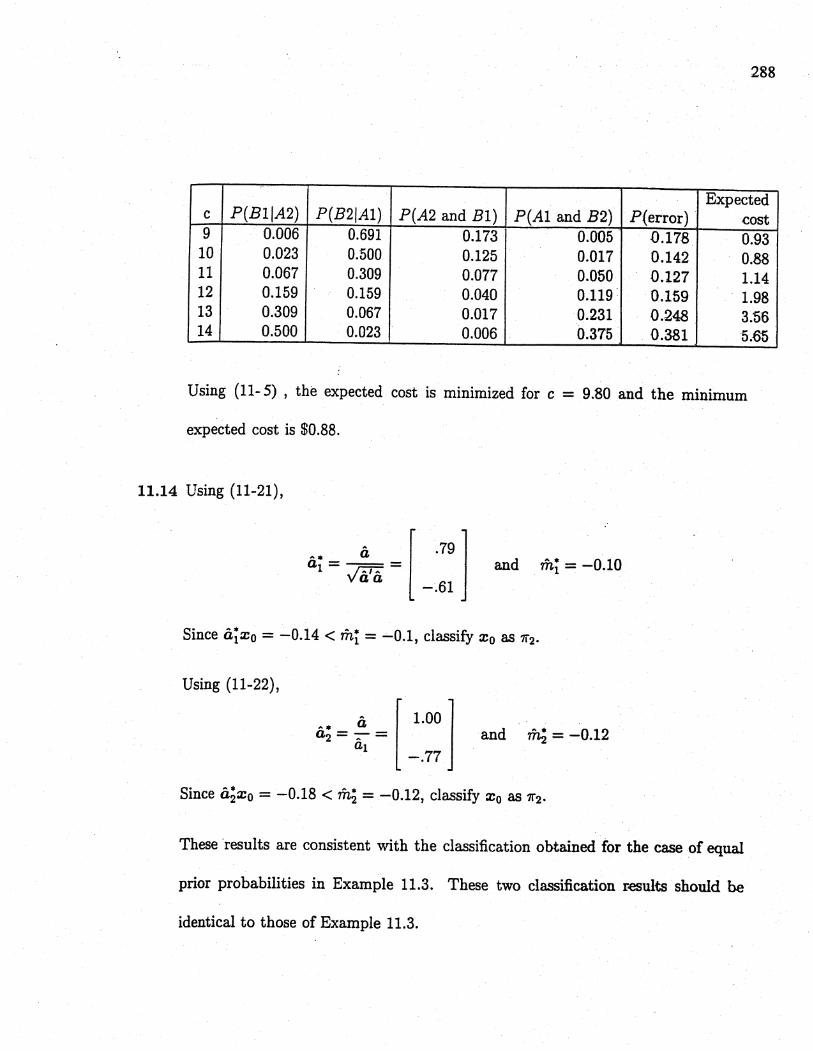
Expectedc P(Bl/A2) P(B2/A1) P(A2 and Bl) P(A1 and B2) P(error) cost9 0.006 0.691 0.173 0.005 0.178 0.93

10 0.023 0.500 0.125 0.017 0.142 0.8811 0.067 0.309 0.077 0.050 0.127 1.1412 0.159 0.159 0.040 0.119 0.159 1.9813 0.309 0.067 0.017 0.231 0.248 3.5614 0.500 0.023 0.006 0.375 0.381 5.65

Using (11- 5) , the expected cost is minimized for c = 9.80 and the minimum

expected cost is $0.88.

11.14 Using (11-21),

â (. 79 1ai - - and m*i = -0.10A* - v'â'â - -.61

Since â~xo = -0.14 ~ rñi = -0.1, classify Xo as 7i2'

Using (11-22),

aA 2* -- a~ --( 1.00 i~ and m; = -0.121 -.77

Since â;xo = -0.18 ~ m; = -0.12, classify Xo as '12.

These 'results are consistent with the classification obtained for the case of equal

prior probabilties in Example 11.3. These two clasification r.eults should be

identical to those of Example 11.3.

11.15

289

f1 (xl (C(lIZl P2JfZ(~) l eT Pi defines the same region as

rc(1IZ) PzJ1n fi(~) -In f2(~) l 1n Le-pi . For a multivariate

normal distribution

1n f.(x) = _12 ln It.1 _.22 ln 2rr - 21(x-ii,.)'r'(x-ii.), i=1,2, - 1 - - , --1so

1 n f1 (~) - , n f 2 (:) = - ~ (:-~1)' ~i 1 (:-~, )

1 ( ) ,+- , 1 ( I t i I)+ 2' ~-!:2 +2 (~-~Z) - '2 1n M

_ 1 ( ,.,-1 '+ -1 , +-1- - i : "'1 : - 2~rl'1 : + ~1 "'1 ~1

, t - , 1 +- 1 ,- 1 1 ( U i/ )- ~ '2 ~ + 2!:2'12~ - !:2+2 !:2) - '21n iW

1 1(+-1 +-1) (,+-1 ,+-1)= - 2 ~ ~1 - '12 ~ + ~1+1 - ~2"'2 ~ - k

where 1k='21n(iii/) 1 i -1 , -1iW + I'!!i+1 ~1 - ~2i2 ~2) .

290

11.16

(f ¡(X)J

Q = In ..fi(x) = - i lnl+il - i(:-~l) 'ti1 (~-~1)

1 l' -1+ '2 In!t21 + 2'(~-~2) t, (~-~2)

1 , (..-1 t- 1 ) i +-, 1+- i= - -2 x +i -+2 X + X t II - _X 1'2 ll_Z - k.. .. - 1..1

where k 1 (1 (I t ii ) 1..-' 't-1 ' J= 2' n ii + ~, 1'1 ~i - ~2T2 ~2 .

When ti = h = t,

Q i -i- 1 1+-1 1 ( i t- 1 1+-1)= ~ l' ~1 -: +~2 - 2' ~i T ~1 - !:21' ~Z

It-'()'( 1+-1 '= ~ l ~1 - LZ - 2' l:i - e2) l (~1 +!:Z)

11.17 Assuming equal prior probabilties and misclassification costs c~2Ii) = $W and

c(1/2) = $73.89. In the table below ,

1Q __ i ("(-i "(-i) (i "(-i i -i)- 2 Xo LJi - ~2 Xo + J.i ~i - 112:E2 :to

-~l (IEil) _ ~( i~-l i -1 )2 n 1~21 2 1-1 i 1-1 - 1-2~2 1-2

291

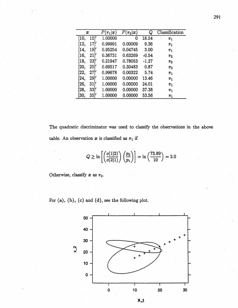
x P('1ilx) P ('12 I x) Q Clasification

(10, 15)' 1. 00000 0 18.54 '1i

(12, 17)' 0.99991 0.00009 9.36 '1i

(14, 19)' 0.95254 0.04745 3.00 '11

(16, 21)' 0.36731 0.63269 -0.54 ii2

(18, 23)' 0.21947 0.78053 -1.27 '12

(20, 25)' 0.69517 0.30483 0.87 1l2

(22, 27)' 0.99678 0.00322 5.74 '1i

(24, 291' 1. 00000 0.00000 13.46 '1i

(26, 31)' 1. 00000 0.00000 24.01 '1i

(28, 331' 1. 00000 0.00000 37.38 '11

(30, 35)' 1.00000 0.00000 53.56 '1i

The quadratic discriminator was used to classify the observations in the above

table. An observation x is classified as '11 íf

Q ~ In r(C(112)) (P2)J = In (73.89) = 2.0L c(211) Pi 10

Otherwise, classify x as '12.

For (a), (b), (c) and (d), see the following plot.

50

400

030 0

00

C\x' 20

10

0

o 10 20 30

)L1

292

11.18 The vector: is an (unsealed) eigen'l.ector of ;-1B since

t-l t-l 1B: = t c(~1-~2)(~1-~2)IC+- (~1-~2)

= c2t-l (~1-~2) (~1-~2) i t-1 (~1-~2)

where

= A t-1 (~1-~2) = A :

A = e2 (~1-~2) 't-l (!:1-~2) .

11.19 (a) The calculated values agree with those in Example 11.7.

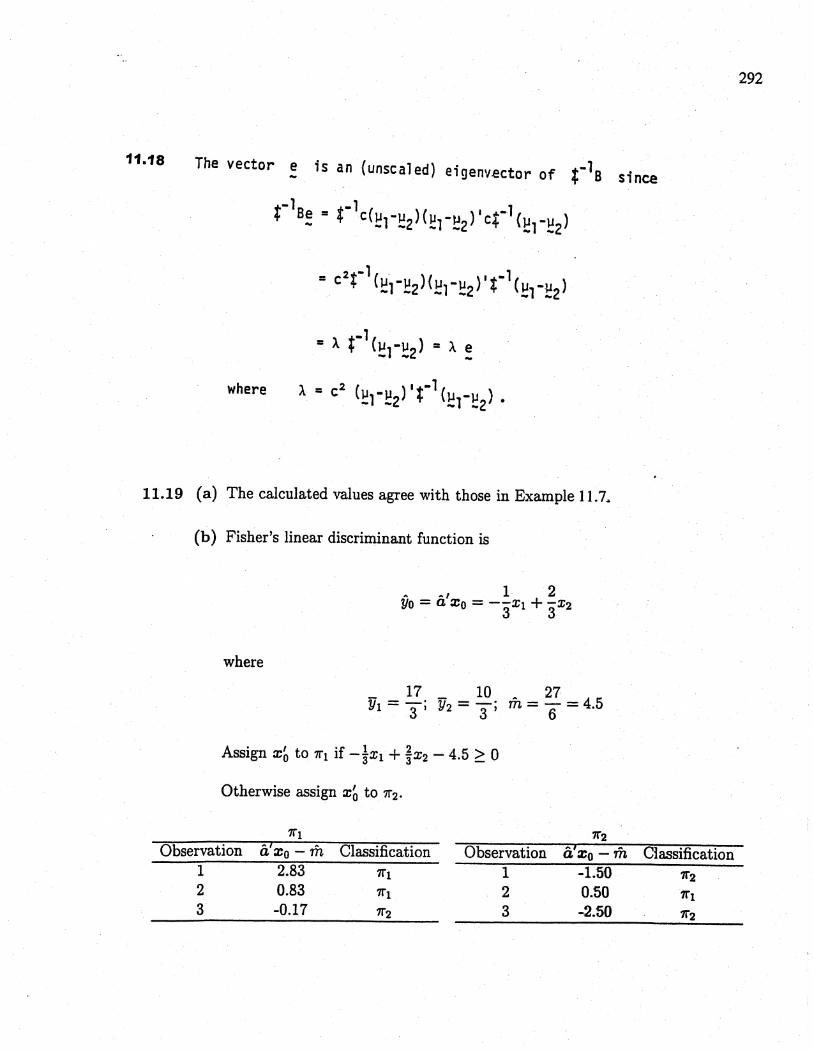
(b) Fisher's linear discriminant function is

A AI 1 2Yo = a Xo = --Xl + -X23 3

where

17 10 27Yl = -; Y2 = -; rñ = - = 4.53 3 6

Assign x~ to '1i if -lxi + ~X2 - 4.5 ~ 0

Otherwise assign x~ to '12.

'1i '12

Observation "'i .. Classification Observation -I .. Classificationa Xo - m a Xo - m1 2.83 '11 1 -1.50 112

2 0.83 '1i 2 0.50 7(1

3 -0.17 '12 3 -2.50 7í2

293

The results from this table verify the confusion matrix given in Example 11.7.

(c) This is the table of squared distances ÎJt( x) for the observations, where

D;(x) = (x - xd8~;oied(X - Xi)

'11 '12

Obs. ,ÎJI(x) ÎJ~ (x) Classification Obs. ÎJ~ (x) ÎJH x ) Clasification

1 i 21'1i 1 13 i 7f23 3 3 3

2 i J! '1i 2 l i 7fi3 3 3 3

3 4 3'12 3 19 4

7f23 3 3 3

The classification results are identical to those obtained in (b)

11.20 The result obtained from this matrix identity is identical to the result of Example

11.7.

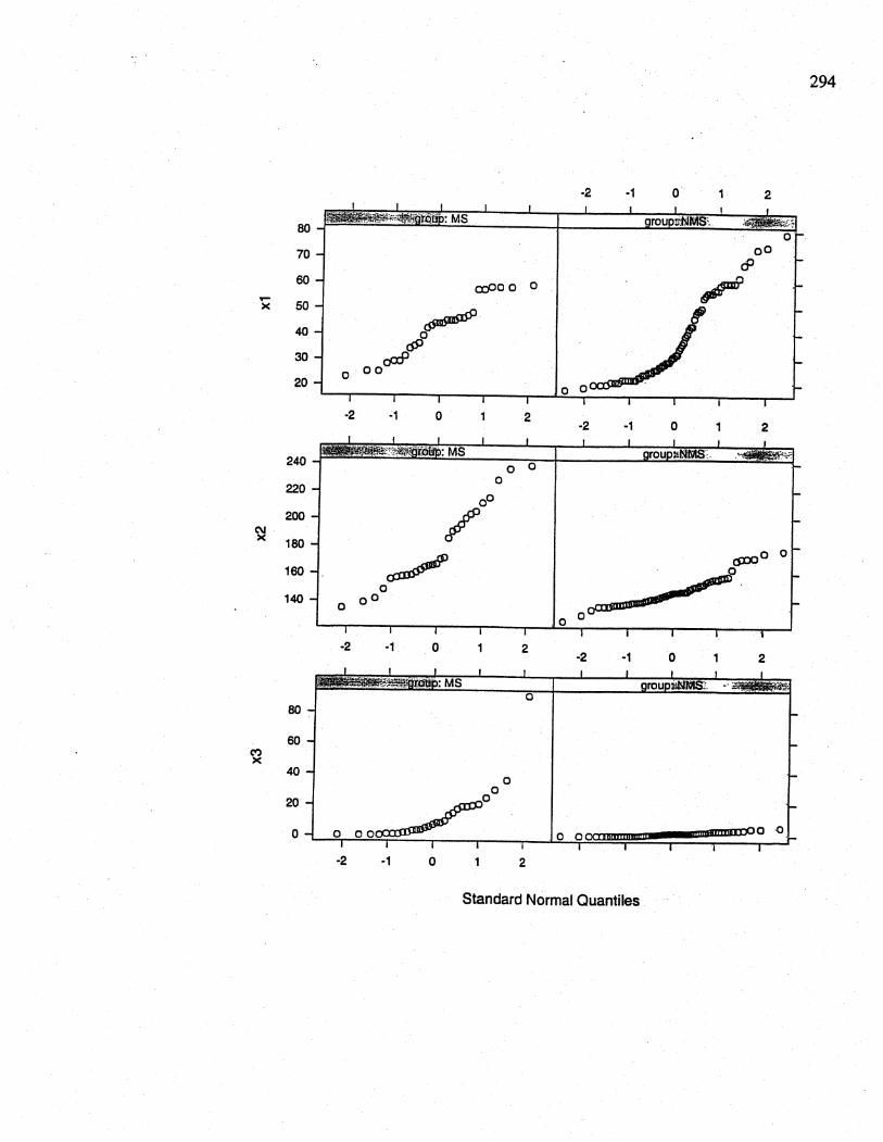
11.23 (a) Here ar the normal probabiHty plot'S for each of the vaables Xi,X'2,Xa, X4,XS

294

-2 .1 o 2

295

-2 -1 0 2

....~a_~

300 00

~ ocPx 250 ~200 00/

0 0

.2 -1 0 2 .2 -1 0 2

80 0

60IIx 40

20

,i.III.ID.ooO 00

.2 -1 0 1 2

Standard Normal Quantiles

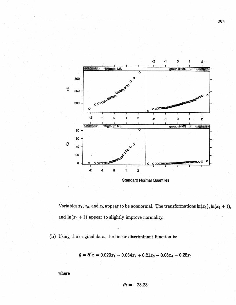
Variables Xi, xa, and Xs appear to be nonnormaL. The transformations In\xi) , In,(x3 + 1),

and In(xs + 1) appear to slightly improve normality.

(b) Using the original data, the linear discriminant function is:

y = â' x = 0.023xi - O.034x2 + O.2lx3 - 0.08X4 - 0.25xs

where

ri = -23.23

Thus, we allocate Xo to Í1i (NMS group) if

296

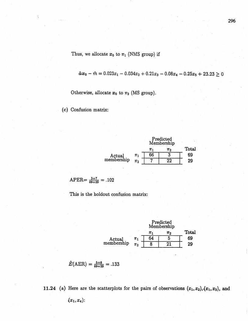
âxo - rñ = 0.023xi - 0.034x2 + 0.2lx3 - 0.08X4 - 0.25xs + 23.23 ;: 0

Otherwise, allocate Xo to '12 (MS group).

( c) Confusion matrix:

Actualmembership

APER= 6~~~9 = .102

;~ j

PredictedMembership'1i '1266 37 22

This is the holdout confusion matrix:

Actualmembership

Ê(AER) = 6~~~9 = .133

;~ j

PredictedMembership,'1i '1264 58 21

Total

t ~~

Total

t ~:

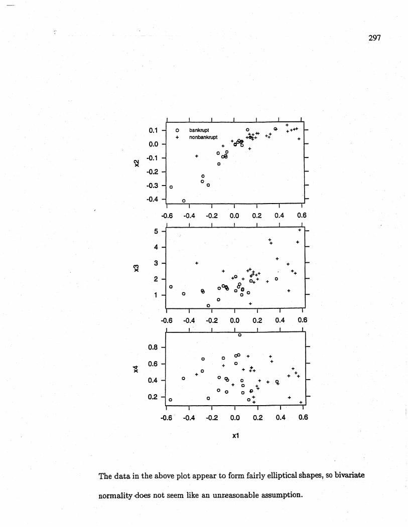
11.24 (a) Here are the scatterplots for the pairs of observations (xi, X2),tXi, X3), and

~Xl' X4):

297

+0.1 0 bankrupt 0 Q. ++++++* +:+ nonbankrupt +it+ +0.0 + +lt

+o 0

.0.1 + ceC\)( 0

-0.20

-0.30

0 0

-0.4

-0.6 -0.4 -0.2 0.0 0.2 0.4 0.6

5 +

+ +4

+

3+

+ +C")( + +; ++

++2 +0 + + 00+ +

0 oOi 8(31 0 ~ 000 +

0+

-0.6 -0.4 -0.2 0.0 0.2 0.4 0.6

0.8

0 0 óJ + +

0.6 0 ++-a + + +)( 0 ++

+ +

0.4 0 o Cò + +0 + + q.+ 0 \0 0 0 Ll

0.2 0 0 0+ ++

-0.6 -0.4 -0.2 0.0 0.2 0.4 0.6

x1

The data in the above plot appear to form fairly ellptical shapes, so bivaate

norma1ìty -does not seem like an unreasonable asumption.

298

(b) '11 = bankrupt firms, '12 = nonbankrupt firms. For (Xi,X2):

( -0,0688 i ' ( 0,0442 0.02847 J

Xi - 8i --0.0819 0.02847 0.02092

X2 -( 0.2354 i '

82 -lO'M735 0.Oæ37 J0.0551 0.00837 0.00231

(c), (d), (e) See the tables of part (g)

(f)

( 0.04594

8 pooled =

0.01751

0.01751 J

0.01077

Fisher's linear discriminant function is

y = â'x = -4.67xi - 5.l2x2

where

rñ = -.32

Thus, we allocate Xo to '1i (Bankrupt group) if

âxo - rñ = -4.67xi - 5.12x2 + .32 ~ 0

Otherwise, allocate Xo to '12 (Nonbankrupt group).

APER= :6 = .196.

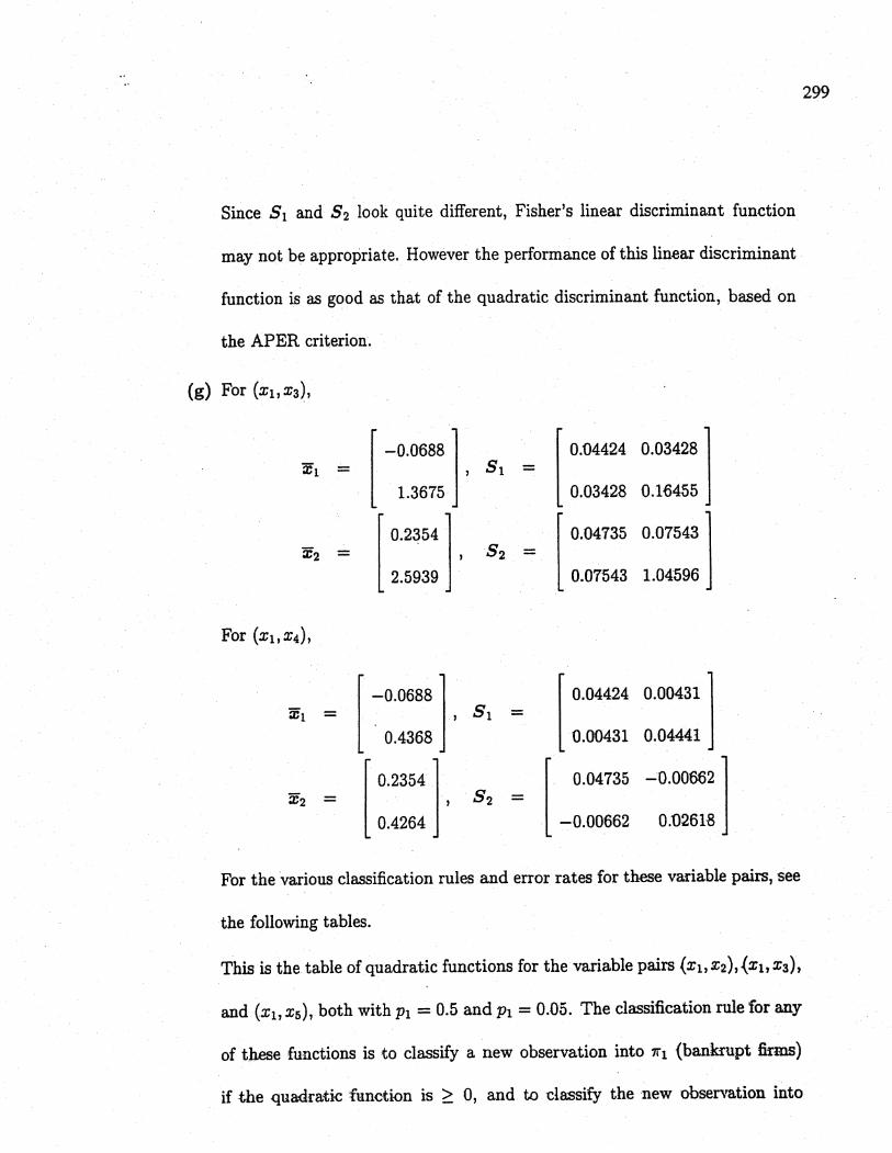
299

Since 8i and 82 look quite different, Fisher's linear discriminant function

For the various classification rules and error rates for these variable pairs, see

the following tables.

This is the table of quadratic functions for the variable pairs .(Xb X2),~Xb X3),

and (Xb xs), both with Pi = 0.5 and Pi = 0.05. The classification rule for any

of thee functions is to classify a new observation into 1ii (bankrupt firms)

if the quadratic function is ~ 0, and to classify the new observation into

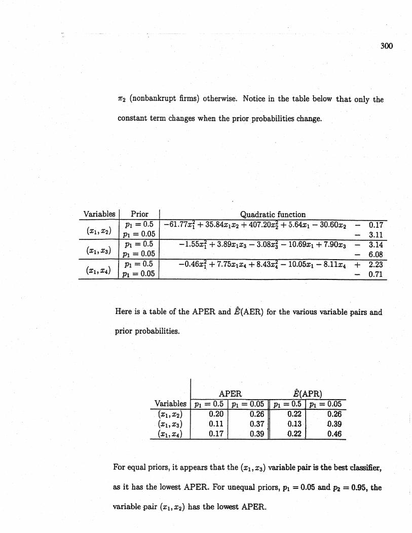
300

'12 (nonbankrupt firms) otherwise. Notice in the table below that only the

constant term changes when the prior probabilties ~hange.

Variables Prior Quadratic functionPi = 0.5 -61.77xi + 35.84xiX2 + 407.20x~ + .s.64xi - 30.60X2 - 0.17

(Xi,X2) Pi = 0.05 - 3.11Pi = 0.5 -i.55x~ + 3.S9xiXa - 3.08x3 - 10.69xi + 7.9ûxa - 3.14

(xi, Xa) Pi = 0.05 - 6.08

(Xl, X4)

Pi = 0.5 -0.46xf. + 7.75xiX4 + 8.43x¡ - 10.05xi - 8.11x4 + 2.23Pi = 0.05 - 0.71

Here is a table of the APER and Ê(AER) for the various variable pairs and

prior probabilties.

APER Ê(APR)Variables Pi = 0.5 Pi = 0.05 Pi = 0.5 Pi = 0.05

(Xi, X2) 0.20 0.26 0.22 0.26

(Xi, xa) 0.11 0.37 0.13 0.39(Xi, X4) 0.17 0.39 0.22 o ,4t)

For equal priors, it appears that the (Xl, Xa) vaiable pair is the best clasifer,

as it has the lowest APER. For unequal priors, Pi = 0.05 and P2 = 0.95, the

variable pair (xi, X2) has the lowet APER.

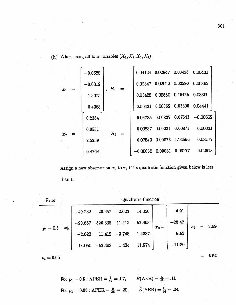
301

(h) When using all four variables (Xb X2l X3, X4),

-0.0688 0.04424 0.02847 0.03428 0.00431

-0.0819 0.02847 0.02092 0.0258D () .00362

Xi - , 8i -1.3675 0.03428 0.02580 0.1'6455 iJ.0330u

0.4368 0.00431 0.00362 0.03300 0.04441

0.2354 0.04735 0.00837 0.07543 -u.00662

0.0551 0.00837 0.u023l 0.00873 D.0003lX2 - , 82 -

2.5939 0.07543 0.00873 1 :04596 0.03177

0.4264 -0.00662 0.00031 0.03177 0.02618

Assign a new observation Xo to '1i if its quadratic function .given below is less

than 0:

Prior Quadratic function

-49.232 -20.657 -2.623 14.050 4.91

-20.657 526.336 11.412 -52.493 -28.42Pi = 0.5 x' xo+ Xo - 2.69

0

-2.623 11.412 -3.748 1.4337 8.65

14.050 -52.493 1.434 11.974 -11.80

Pi = 0.05- 5.64

For Pi = 0.5 : APER = ;6 = .07, Ê(AER) = ;6 = .11

For Pi = D.n5 : APER = :6 = .20, Ê(AER) = ¡~= .24

302

11.25 (a) Fisher's linear discriminant function is

Yo = a' Xo - rñ = -4.80xi - 1.48xg + 3.33

Classify Xo to '1i (bankrupt firms) if

a' Xo - rñ ;: 0

Otherwise classify Xo to '12 (nonbankrupt firms).

The APER is 2:l4 = .13.

, This is the scatterplot of the data in the (xi, Xg) coordinate system, along

with the discriminant line.

5

4

3C'x

2

1

-0.6 -0.4 -0.2 0.0 0.2 0.4 0.6

x1

(b) With data point 16 for the bankrupt firms delete, Fisher's linear discrimit

303

function is given by

Yo = a'a;O - m = -5.93xi - 1.46x3 + 3.31

Classify Xo to'1i (bankrupt firms) if

a'xo - m, 2: 0

Otherwise classify Xo to '12 (nonbankrupt firms).

The APER is 1;;4 = .11.

With data point 13 for the nonbankrupt firms deleted, Fisher's linear dis-

criminant function is given by

Yo = a'xo - m = -4.35xi - i.97x3 + 4.36

Classify Xo to '1i (bankrupt firms) if

a/:.o - m ;: 0

Otherwise classify Xo to '12 (nonbankrupt firms).

The APER is 1;;3 = .089.

This is the scatterplot of the observations in the (Xl, X3), coordinate system

with the discriminant lines for the three linear discriminant functions given

abov.e. Als laheUed are observation 16 for bankrupt firms and obrvtion

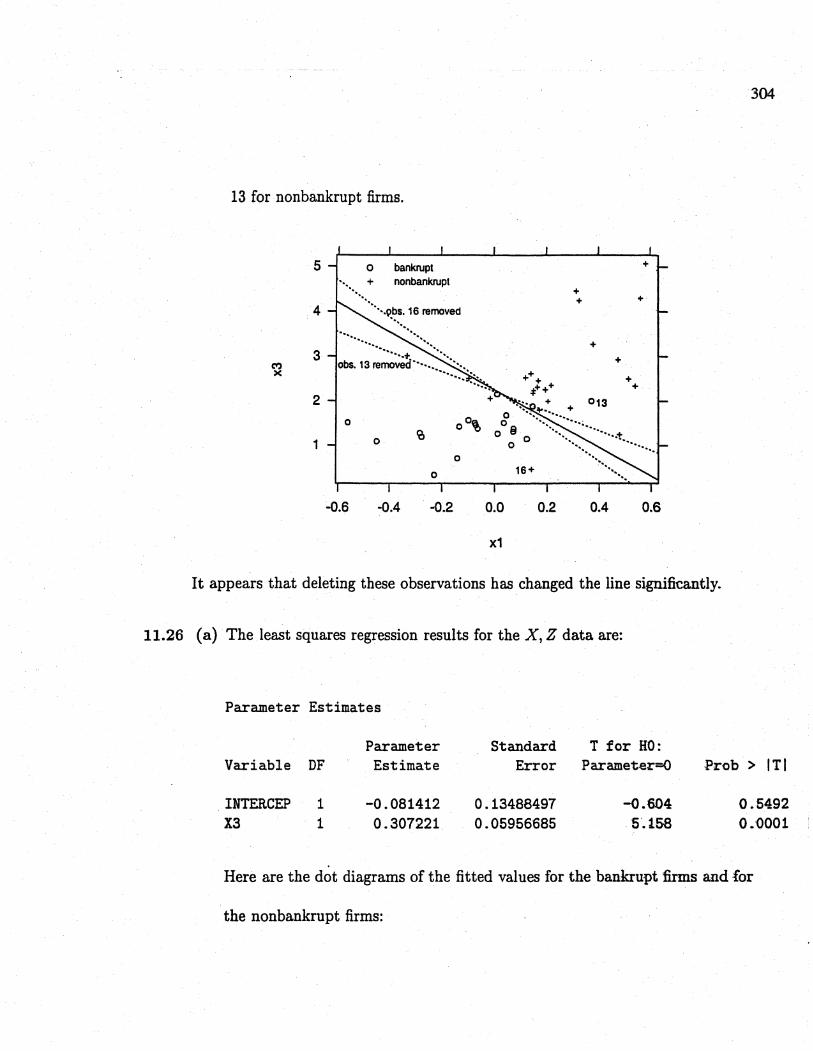
304

13 for nonbankrupt firms.

It appears that deleting these observations has changed the line signficantly.

11.26 (a) The least squares regression results for the X, Z data are:

Parameter Estimates

Parameter Standard T for HO:

Variable DF Estimate Error Paramet-er=O Prob ;) ITI

INTERCEP 1 -0.081412 o . 13488497 -0.604 o .5492X3 1 0.307221 o .05956685 5.158 0.0001

Here are the dot diagrams of the fitted values for the bankrupt fims and for

the nonbankrupt firms:

305

. . . .. .. . . . . ..+~--------+---------+---------+---------+---------+----- --Banupt

. . .. .. . .....+---------+---------+--- ---- --+---------+---------+----- - - N onbanrupto . 00 0 . 30 O. 60 0 .90 1. 20 1.50

This table summarizes the classification results using the fitted values:

OBS GROUP FITTED CLASSIFICATION---------------------------------------------131631343841

banruptbanruptnonbankrnonbanrnonbanrnonbanr

o . 57896

0.531220.47076O. 06025o .48329o . 30089

misclassifymisclassifymisclassifymisclassifymisclassifymisclassify

The confusion matrix is:

Actualmembership

PredictedMembership'11 '12

'11 =1 19 2'12 J 4 21

Total

t ;;

Thus, the APER is 2:t4 = .13.

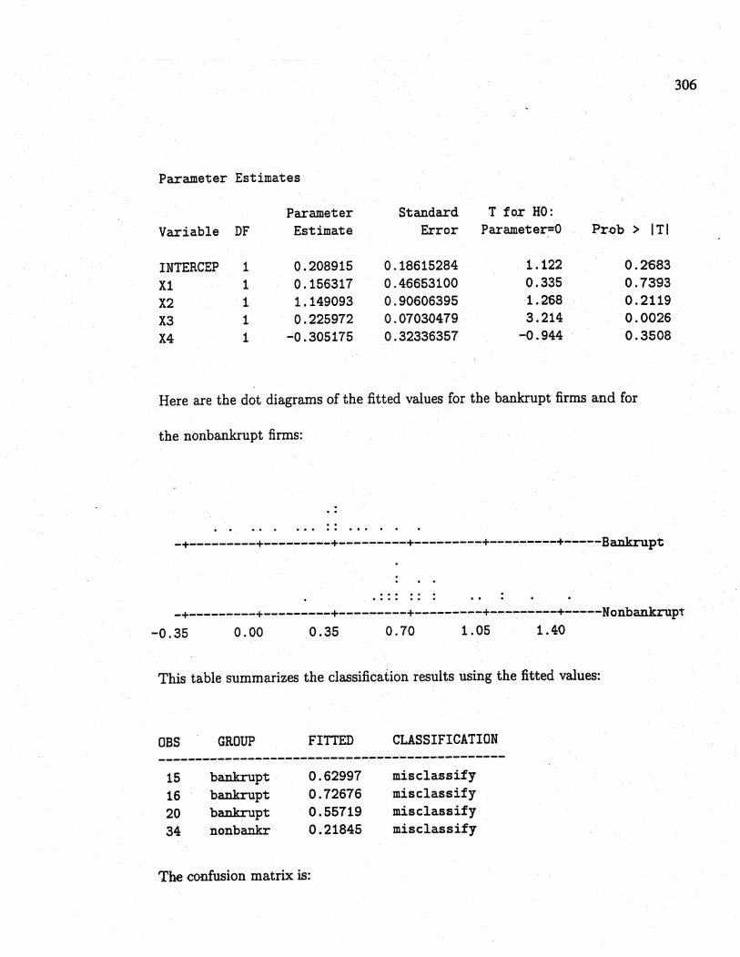
(b) The least squares regression results using all four variables Xi, X2, X3, X4 are:

306

Parameter Estimates

Parameter Standard T fo.r HO:

Variable DF Estimate Error Parameter=O Pr.ob ;) ITI

INTERCEP 1 0.208915 0.18615284 1.122 O. 2ô83

Xl 1 o . 156317 0.46653100 0.335 o .7393

X2 1 1. 149093 o . 90606395 1.268 0.2119X3 1 o . 225972 0.07030479 3.214 o . 0026

X4 1 -0.305175 0.32336357 -0 .944 O. 3508

Here are the dot diagrams of the fitted values for the bankrupt firms a:nd for

the nonbankrupt firms:

_+_________+_________+_________+_________+_________+__---Banrupt

_+_________+_________+_________+_________+_________+__---N onbankrupt

-0.35 0 . 00 0 .35 0 . 70 1 .05 1.40

This table summarizes the classification results using the fitted values:

OBS GROUP FITTD CLASSIFICATION----------------------------------------------

15 banrupt o . 62997 misclassify16 banrupt o . 72676 misclassify20 banrupt 0.55719 misclassify34 nonbanr 0.21845 misclassify

The confusion matrix is:

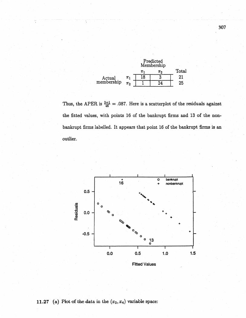
307

Actualmembership :~ j

PredictedMembership'1i '1218 31 24

Total

F ;~

Thus, the APER is 3::1 = .087. Here is a scatterplot of the residuals against

the fitted values, with points 16 of the bankrupt firms and 13 of the non-

bankrupt firms labelled. It appears that point 16 of the bankrupt firms is an

outlier.

+ 0 bankrupt16 + nonbankrupt

0.5 +."-

~In 0 "'~-e °:i"C 0.0 Cò +'ëi 0 +(I .c: ~ +,

°eo +-0.5 °

° 130

0.0 0.5 1.0 1.5

Fitted Values

11.27 ~a) Plot'Üfthe4ata in the (Xi,X4) variabte space:

308

:2~

,'§Ii-Q)i:-

'VX

2.5 :;:; :; :;

:; :; :; :; :;:; :; :;:; :; :; :;

2.0 :; :; :; :; :;:; :; :;:; :; :; :; :; :; .:; +

+ :; + +1.5 Jo + .++++:;++++++

+ + + + + ++ + + +

1.0 ++ ++++ ++ o

+~

SetosaVersiclorVirginic

0.5o

o

o o 000 0o 00 00000000000 0 000 0 02.0 2.5 3.0 3.5 4.0

X2 (sepal width)

The points from all three groups appear to form an ellptical 'Shape. However,

it appears that the points of '11 (Iris setosa) form an ellpæ with a different

orientation than those of '12 (Iris versicolor) and 113 (Iri virginica). This

indicates that the observations from '1i may have a different covariance matrix

from the observations from '12 and '13.

(b) Here are the results of a test of the null hypothesis Ho : Pi = 1L2 = ¡.3 vel'US

Hi : at least one of the ¡.¡'s is different from the others at the a = 0.05 level

of significance:

Statistic Value F Num DF Den DF Pr)J F

WiJ.x'S' Lambda o .~2343B63 199.145 8 288 Q.0001

309

Thus, the null hypothesis Ho : J11 = J12 = J13 is æjected at the Q = 0.05

level of significance. As discussed earlier, the plots give us reason to doubt

the assumption of equal covariance matrices for the three groups.

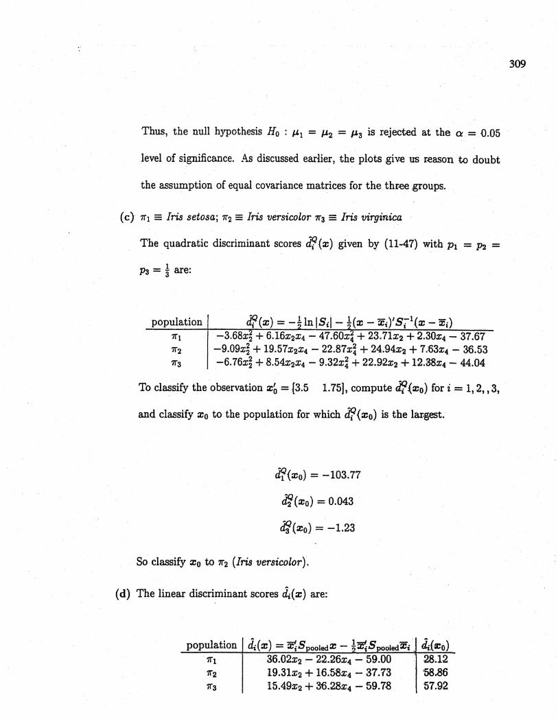
(c) '11= Iris setosa; '12 = Iris versicolor '13 = Iris virginica

The quadratic discriminant scores d~(x) given by (11-47) with Pi = P2 =

P3 = l are:

population'11

'12

'13

~(x) = _1 In ISil- l(x - Xi)' Sii(x - Xi)-3.68X2 + 6.16x2x4 - 47.60x4 + 23;71x2 + 2.30X4 - 37.67

-9.09x~ + 19.57x2x4 - 22.87x~ + 24.94x2 + 7..ß3x4 - 36.53-6. 76x~ + 8.54x2X4 - 9.32x~ + 22.92x2 + 12.38x4 - 44.04

To classify the observation x~ - 13.5 1.75), compute Jftxo) for i = 1,2,,3,

and classify Xo to the population for which ~(xo) is the la¡;g.et.

AQ

di (xo) = -103.77AQ

d2 (xo) = 0.043

cf(xo) = -1.23

So classify Xo to '12 (Iris versicolor).

(d) The linear discriminant scores di(x) are:

population I di(x) = ~SpooledX - l~Spooledæi J dïÍ2;O)

1li . 36.02x2 - 22.26x4 - 59.00 .28.12'12 i9.3lx2 + 1£.58x4 - 37.73 '58..6'13 15A9X2 + 3'6.28x4 -59.78 57.92

310

Since d¡(xo) is the largest for í = 2, we classify the new observation x~ =

i3.5 1.75) to'1i according to (11-52). The results are the same for (c) and

(d).

(e) To use rule (11-56), construct dki(X) = dk(x) - di(æ) for all i "It. Then

classify x to'1k if dki(X) ;: 0 for all i = 1,2,3. Here is a table of dn(%o) for

i, k = 1,2,3:

1i2 3

1

J 2i

0 -30.74 -29.8030.74 0 0.9429.80 -0.94 0

Since dki(XO) .;: 0 for all i =l 2, we allocate Xo to '12, using (11-52)

Here is the scatterplot of the data in the (X2' X4) variable space, with the

classification regions Ri, R2, and Rg delineated.

2.5 :; ;.:; ;. :;

:; :; ;. :; :;;. :; ;.:; ;. ;. :;

2.0 :; :; :; :; ;.;. ;. :;- :; ;. :; ;. ;. ;. ;i.i :;-U + ;. + +.~

1.5 . + ;i++++eØ

;.+++++++ + + + + +

ã5 + + + +Co- 1.0 +'"X

::0

0.5 00 000 0

0 00 00000000000 0 000 0 0

2.0 2.5 3.0 3.5 4.0

X2 ~sepal width)

311

36 CHAPTER 11. DISCRIMINATION A.ND CLASSIFIC.4.TIOH

(f) The APER = ii~ = .033. Ê(AER) = itg = .04

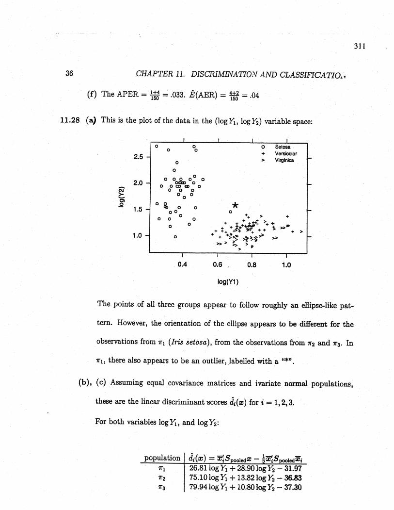
11.28 (a) This is the plot of the data in the (lOgYi, 10gY2) variable space:

0 00 02.5

00

2.00 o 0 00 0Oll 0- 0 OCDai 0

~ 0 0 0- 00 0Cl 0

!b.Q1.5 0 0

00 00 0 00 0

1.0 0

o Setosa+ Versiclor~ Virginic

*o ++;. ++ +;.

+ t +.t;t + + :P+:t + J: V + + t ;. + ;.+ +~ +;.+ +;.~ ;.'l~~ ;.;.;.;. ;.;.;. ;.;. ;')l;.

0.4 0.6 , 0.8 1.0

log(Y1 )

The points of all three groups appear to follow roughly an eliipse-like pat-

tern. However, the orientation of the ellpse appears to be different for the

observations from '11 (Iris setósa), from the observations from '12 and '13. In

'1i, there also appears to be an outlier, labelled with a "*".

(b), (c) Assuming equal covariance matri.ces and ivariate normal populations,

these are the linear discriminant -scores dit x) for i = 1, 2, 3.

For both variables log Yi, and log 1':

population J df(X) = ä;SpooledX - lä;SpooledZi

'11 . 26.81 log Yi + 28.90 log 1' - 31.97

7r2 75.10 log Yí + 13.82 log 1' - 36.83

7r3 79.94 log Yi + 10.80 IQg Y2 - 37.30

312

For variable log Yi only:

population'1i

'12

'13

¿¡(x) = ~SpooledX - læ~Spooleåæi

40.90 log Yi - 7.82

81.84 log Yi - 31.3085.20 log Yi - 33.93

For variable 10gY2 only:

population ¿¡(x) = ~SpooiedX - l~Spooledæi

'11 30.93 log Y2 - 28.73'12 19.52 log Y2 - 11.44'13 16.87 log Y2 + 8.54

Variables APER E(AER)

log Yl, log Y226 - 17 27 - 18150 - . 150 - .

log Yl 49 - 33 49 - 33iš -. 150 - .

log Y2,34 - 23 34 - 23i50 - . i50 - .

The preceeding misclassification rates are not nearly as good as those in Ex:-

ample 11.12. Using "shape" is effective in discriminating'1i (iris versicolor)

from '12 and '13. It is not as good at discriminating 7í2 from 1i3, because of

the overlap of '11 and '12 in both shape variables. Therefore, shape is not an

effective discriminator of all three species of iris.

(d) Given the bivarate normal-like scatter and the relatively largesamples, we do not expect the error rates in pars (b) and,(c) to differ.much.

313

11.29 (a) The calculated values of Xl, Xi, X3, X, and Spooled agree with the results for

these quantities given in Example 11.11

(b)

w-i _

( 0.348899 0.000193) _

, B -0.000193 .000003

( 12.'501518.74

1518.74 J

258471.12

The eigenvalues and scaled eigenvectors of W-l Bare

).i 5.646,A'

( 5.009 J

- ai -0.009

).2 0.191,A i

( 0'2071

- a2 --0.014

To classify x~ = (3.21 497), use (11-67) and compute

EJ=i(âj(x - Xi))2 i = 1,2,3

Allocate x~ to '1k if

EJ=i(âj(x - Xk))2 ::E;=i (âj(æ - Xi))2 for alli i= Ie

For :.o,

k L~_l(â'.(X - Xk)J2

1 2.632 16.993 2.43

Thus, classify Xo to '13 This result agrees with thedasifiation given in

Example 11.11. Any time there are three populations with only two discrim-

314

inants, classification results using Fisher's Discriminants wil be identical to

those using the sample distance method of Example 11.11.

11.30 (a) Assuming normality and equal covariance matrices for the three populations

'1i, '12, and '13, the minimum TPM rule is given by:

Allocate xto '1k if the linear discriminant score dk (x) = the largest of di (:.), d2 \ æ ), d3\~

where di(x) is given in the following table for i = 1,2,3.

population'11

'12

'13

di(x) = ~SpooledX - lX~SpooledXi

0.70xi + 0.58x2 - l3.52x3 + 6.93x4 + 1.44xs - 44.78

1.85xi + 0.32x2 - 12.78x3 + 8.33x4 - 0.14xs - 35.20

2.64xi + 0.20X2 - 2.l6x3 + 5.39x4 - 0.08xs - 23.61

(b) Confusion matrix is:

PredictedMembership

'1i '12 '13 Total711

38

Actual '11membership '12

7í3

7 0 0

1 10 0

0 3 35

And the APER O+5~+3 = .071

The holdout confusion matrix is:

PredictedMembership

'1i '12 '13 Total

me~~~~hiP :: J ~ I ~ 1 :5 ( ~

E(AER)= 2+5~+3 = .125

315

(c) One choice of transformations, Xl, log X2, y', log X4,.. appears to improve the

normality of the data but the classification rule from these data has slightly higher

error rates than the rule derived from the original data. The error rates (APER,

Ê(AER)) for the linear discriminants in Example 11.14 are also slightly higher

than those for the original data.

11.31 (a) The data look fairly normaL.

50000

0 00 0

0 c6 0 0

450 0 Q)- 0 0 0 0 +Q) 00 0 00

õJ°i: 0 0 0 0+"t +cø 0 00 +:: 400 0000 0 + + +- 0 °õJ + 't0 + + +C\ +

Gl+ + + +

X + .¡+ +0 +0 +

+ +

350 1+ 0+ + ++++ ~it + +

+ + +ta Alaskan

300 + Canadian + +

60 80 100 120 140 160 180

X1 (Freshwater)

Although the covariances have different signs for the two groups, the corr.ela-

tions are smalL. Thus the assumption of bivariate normal distributions with

.equal -covariance matrioes does not seem unreasnable.

316

(b) The linear discriminant function is

â'x - rñ = -0.13xi + 0.052x2 - 5.54

Classify an observation Xo to'1i (Alaskan salmon) if â'xo-m ;: 0 and clasify

Xo to '12 (Canadian salmon) otherwise.

Dot diagrams of the discriminant scores:

. .. .

... I... .

-------+---------+---------+---------+---------+--------- Alaskan

. . . .. .. ... . ... . " ........... " . .. .. . . . . .

-------+---------+---------+---------+---------+---------Canadian-8.0 -4.0 0.0 4.0 8.,Q 12.0

It does appear that growth ring diameters separate the two groups reasonably

well, as APER= ~t~ = .07 and E(AER)= ~t~ = .07

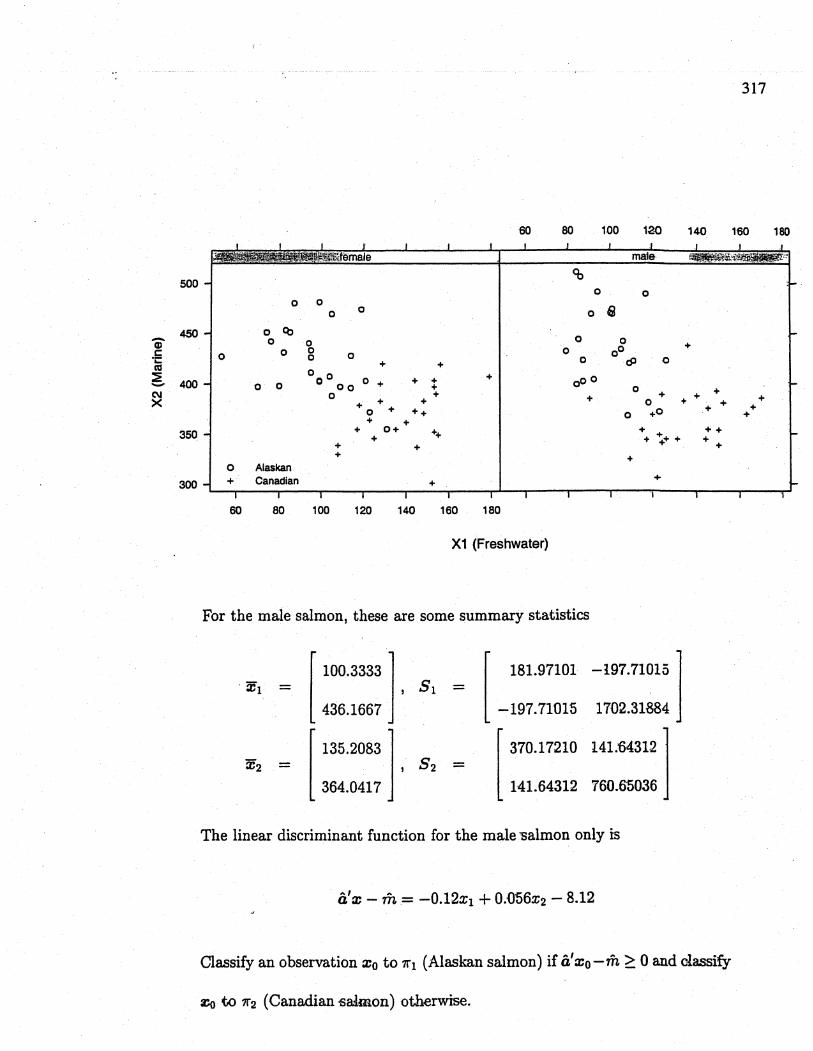
( c) Here are the bivariate plots of the data for male and female salmon separately.

- 45CIi: 0.¡:cte 400C\X

350

500

300

eo 80 100 12.0i

mae ¡~:~:%~~;.~"E~"

160 180

% o 00 0

0 0

0 Cb0 0

0 0 00

o il

140

+

o+ + o

000+

o + + +o + ++0 +

:c to '12 (Canadian -salmon) oth.erwIse.

+

317

++

++ ++

+

Classify an observation Xo to 1ii (Alaskan salmon) if â'xo-m;: 0 and clasify

o o00

óJo

o 0o 0o 000+

o + + +o + +++ +0+ ++ +

+ :.+ +

++ +++

o

++

140 160 180

X1 (Freshwater)

For the male salmon, these are some summary statistics

. xi

( 100.3333 i, Si436.1667

( ::::::: l' S2

( 181.97101 -ì97.71015 J-197.71015 1702.31884

( 370.17210 141:643121141.64312 760.65036

X2

The linear discriminant function for the male 'Salmon only Is

â'x - m= -0.12xi + 0.D56x2 - 8.12

318

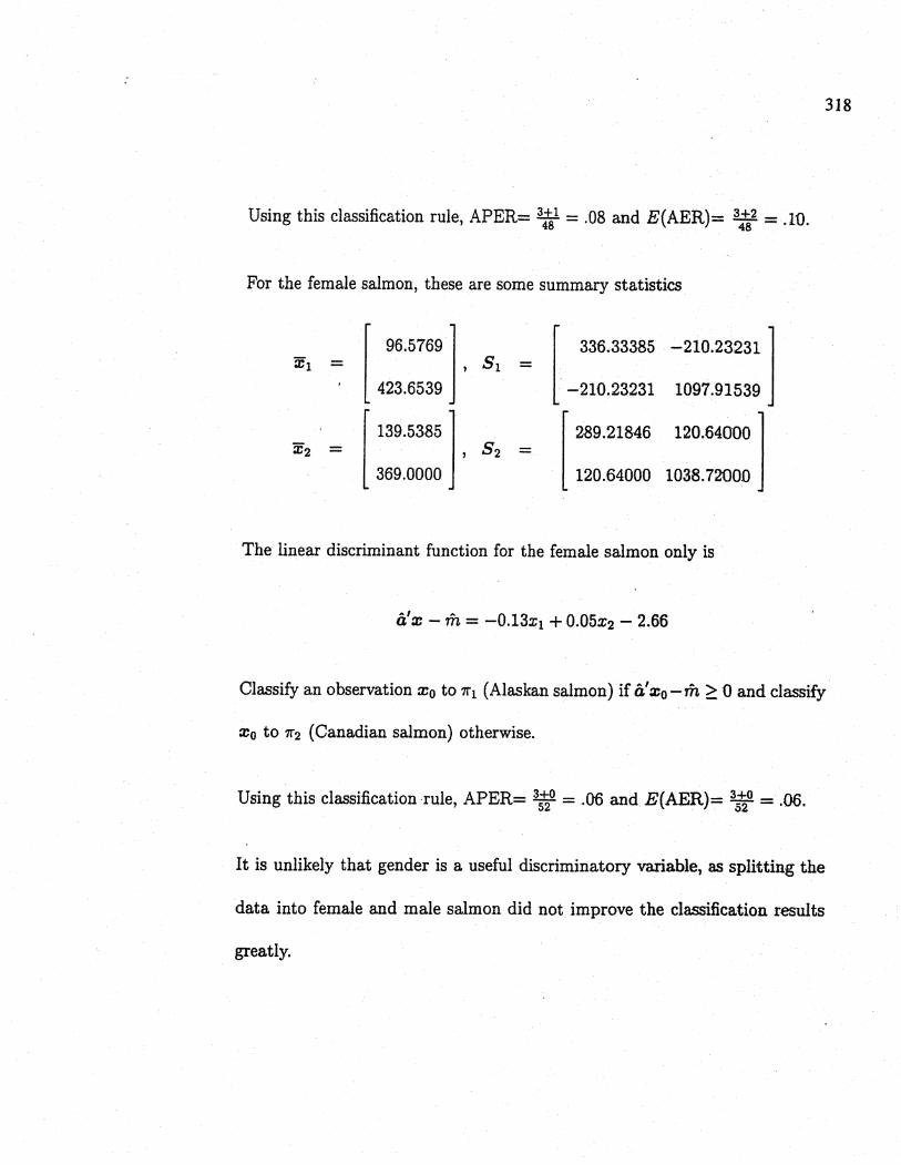
Using this classification rule, APER= 3tal = .08 and E(AER)= 3:ä2 = .w.

For the female salmon, these are some summary statistics

Z¡ - (4::::::: J' s, -

Z2 - (:::::::: J' S2 -

( 336.33385 -210.23231 i-210.23231 1097.91539

( 289.21846 120.64000 J120.64000 1038.72ûOO

The linear discriminant function for the female salmon only is

â' X - rñ = -O.13xi + O.05X2 - 2.66

Classify an observation xo to'1i (Alaskan salmon) if â'xo-m ~ 0 and classify

xo to '12 (Canadian salmon) otherwise.

Using this classification rule, APER= 3i;0 = .06 and E(AER)= 3;;0 = .06.

It is unlikely that gender is a useful discriminatory varable, as splitting the

data into female and male salmon did not improve the classification results

greatly.

319

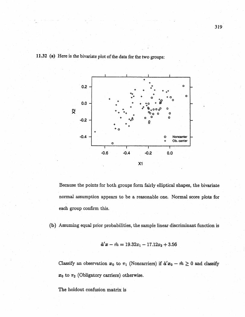
11.32 (a) Here is the bivarate plot of the data for the two groups:

0.2

++

+ 0++ + + + ++

++ +++ + 0 + 0 0

+

+ ã'0+ + + +0+

+ +++ + %+ooo' 0

++ ++ ll 0 0 0+

+++õ 0 0 0

+ + e+

+ 0

0.0

C\X

-0.2

+

-0.4 o Noncrrer+ Ob. airrier

o

-0.6 -0.4 -0.2 0.0

X1

Because the points for both groups form fairly ellptical shapes, the bivariate

normal assumption appears to be a reasonable one. Normal -score plot-s fDr

each group confirm this.

(b) Assuming equal prior probabilties, the sample linear discriminant function is

â'x - ri = i9.32xi - l7.l2x2 + 3.56

Classify an observation Xo to '1i (Noncarriers) if â'xo - rñ ;: .0 and classify

Xo to '12 (Obligatory carriers) otherwise.

The holdout confusion matrix is

Ê(AER)= 4is8 = .16

Actualmembership

'11 j

'12

320

PredictedMembership'1i '1226 48 37

Total

t ~~

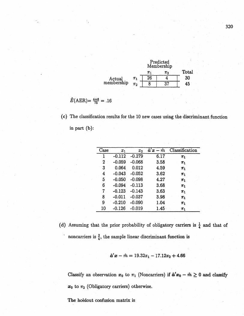
(c) The classification results for the 10 new cases using the discriminant function

in part (b):

Case1

2

3

4

5

6

78

9

10

Xl

-0.112-0.0'590.064

-0.043-0.050-0.094-0.123-0.011-0.210-0.126

X2

-0.279-0.0680.012

-0.052-0.098-0.113-0.143-0.037-0.090-0.019

â' x - rñ Classification

6.17 '1i3.58 '1i4.59 1113.62 lii4.27 '113.68 '1i3.63 lii3.98 '111.04 7íi1.45 '11

(d) Assuming that the prior probabilty of obligatory carriers is ~ and that of

, noncarriers is i, the sample linear discriminant function is

â':. - rñ = 19.32xi - 17.12x2 + 4.66

Classify an observation Xo to lii (Noncarriers) if â':.o - rñ :; 0 and classify

::o to '12 (Obligatory carriers) otherwise.

The hold.ut confusion matrix is

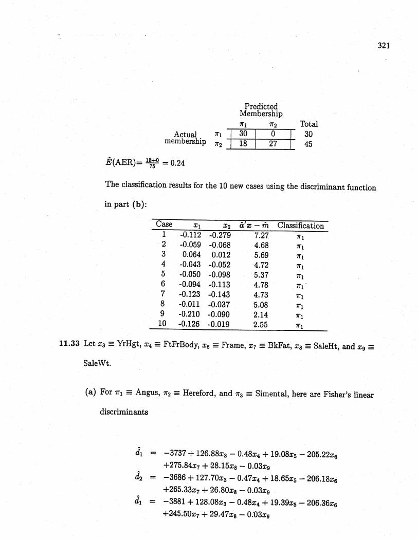
Actualmembership

Ê(AER)= l~tO = 0.24

321

PredictedMembership'11 '12

:: j ~~ I 2°7

Total

t ~~

The classification results for the 10 new cases using the discriminant function

in part (b):

Case1

2

3

45

6789

10

Xi

-0.112-0.0590.064

-0.043-0.050-0.094-0.123-0.011-0.210-0.126

X2

-0.279-0.0680.012

-0.052-0.098-0.113-0.143-0.037-0.090-0.019

â'x - ri

7.274.685.694.725.374.784.735.082.142.55

Classification7ri

'1i

'11

'11

7ri

'1i

'11

'1i

'11

'11

11.33 Let X3 = YrHgt, X4 = FtFrBody, X6 = Frame, X7 = BkFat, Xa = SaleHt, and Xg =

SaleWt.

(a) For '11 = Angus, '12 = Hereford, and '13 = Simental, here are Fisher's linear

discriminants

di -

d2 -

cÎi -

-3737 + l26.88X3 - 0.48X4 + 19.08x5 - 205.22x6

+275.84x7 + 28.l5xa - 0.03xg

-3686 + l27.70x3 - 0.47X4 + l8.65x5 - 206.18x6

+265.33x7 + 26.80xa - 0.03xg

-3881 + l28.08x3 - 0.48x4 + 19.59xs - 206.36x6

+245.50X7 + 29.47xa - 0:03xg

322

When x~ = (50,1000,73,7, .17,54, 1525J we obtain di = 3596.31, d2 = 3593.32,

and d3 = 3594.13, so assign the new observation to '12, Hereford.

This is the plot of the discriminant scores in the two-dimensional discriminant

space:

00 0

20

0 ~00 0

8000 ~00 :.

0 ~- + 0 + i. :.~ct.r 0 ++ + % 0 eO ?:. :.

i :.C\ + :. :.:. :.;: 0+ .p ~

+ + :. :."b ~

-1~ ~

+0 0 :.00 +

+ 0 +:. 0 Angus

.2 + + Hereford+ :. Simental

-2 0 2 4

y1-hat

(b) Here is the APER and Ê(AER) for different subsets of the variable:

Subset I APER Ê(AER)X3, X4, XS, X6, X7, Xai Xg .13 .25

X4, Xs, X7, Xa .14 .20XS, X7, Xa .21 .24

X4,XS .43 .46X4,X7 .36 .39X4,Xa .32 .36X7,XS .22 .22XS,X7 .25 .29Xs,XS .28 .32

11.34 For '11 = General Mils, '12 = Kellogg, and '13 = Quaker and assuming multivariate

flmai data with a 'Cmmon covariance matdx,eaual costs, and equal pri,thes

323

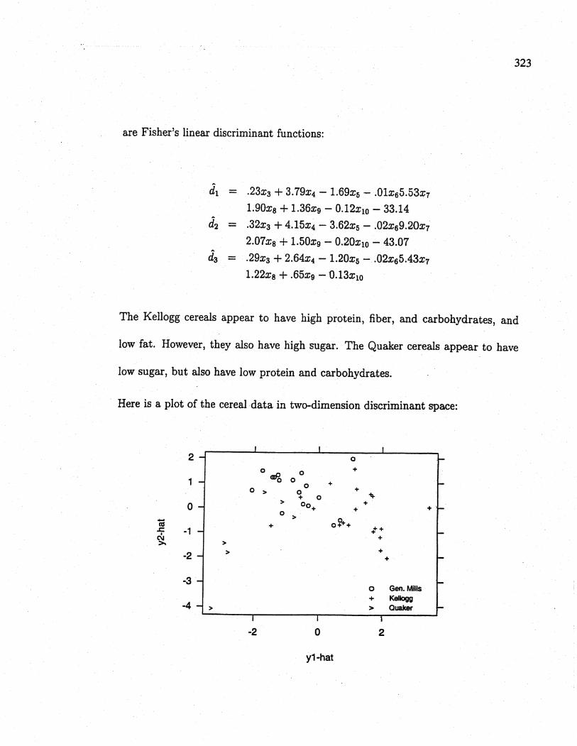
are Fisher's linear discriminant functions:

di

d2 -

d3 -

.23x3 + 3.79x4 - 1.69xs - .Olx65.53x7

1.90XB + 1.36xg - O.12xio - 33.14

.32x3 + 4.l5x4 - 3.62xs - .02X69.20X7

2.07xB + 1.50xg - 0.20xio - 43.07

.29x3 + 2.64x4 - 1.20xs - .02x65.43x7

1.22xB + .65xg - ü.13xio

The Kellogg cereals appear to have high protein, fiber, and carbohydrates, and

low fat. However, they also have high sugar. The Quaker cereals appear to have

low sugar, but also have low protein and carbohydrates.

Here is a plot of the cereal data in two-dimension discriminant space:

2 0o ar +0

1 0 0 +00 0 +;: ~+ 00

;: 00+ ++ +

0 ;:o~++

-lU +

.t +.c -1i+C\;: ;:

;: +-2 +

-3Gen. Mils0

+ Kellog-4 ;: ;: auar

-2 0 2

y1-hat

324

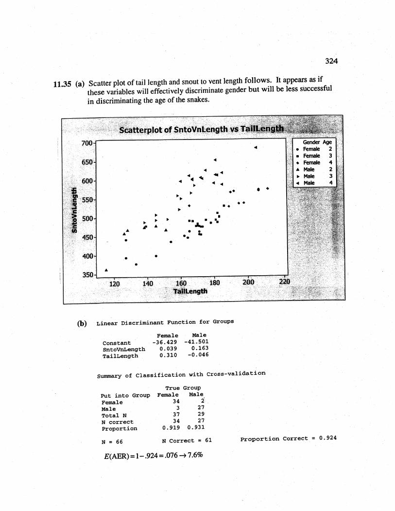
11.35 (a) Scatter plot of tail length and snout to vent length follows. It appears as ifthese variables wil effectively discriminate gender but wil be less successfulin discriminating the age of the snakes.

,:':___::.....-.-' _ _." ..-...-----...----...--...-.. _ _.d:-'..d..d."--"

. Sêatterplotof SntoVnLength.vs Ta.

..

.

..

.... .... .... ..

~.. ..

~ ..~

~

.

. . .. .

~~

.~

.~ .. . .

~ .a . .il . . . ... ..

.

...

140160 180liàjlLength

OD) Linear Discriminant Function for Groups

ConstantSntoVnLengthTailLength

Female-36.429

0.0390.310

Male-41.501

0.163-0.046

..

. .

sumary of Classification with Cross-validation

Put into GroupFemaleMaleTotal NN correctProportion

N = 66

TrueFemale

343

3734

0.919

GroupMale

i272927

0.931

N Correct = 61

E(AER) = 1 - .924 = .076 ~ 7.6%

Proportion Correct 0.924

325

(e) Linear Discriminant Function for Groups

ConstantSntoVnLengthTai lLength

2-112.44

0.330.53

3

-145.760.380.60

4-193.14

0.450.65

sumary of Classification with Cross-validationTrue Group

Put into Group 2 3 4

2 13 2 0

3 4 21 2

4 0 3 21Total N 17 26 23N correct 13 21 21proportion 0.765 0.808 0.913

N = 66 N Correct = 55 Proportion Correct 0.833

E(AER)= 1-.833= .167 ~ 16.7%

(d) Linear Discriminant Function for Groups

2

Constant -79.11SntoVnLength 0.36

3-102.76

0.41

4-141. 94

0.48

sumry of Classification with Cross-validationTrue Group

Put into Group 2 3 42 14 1 0

3 3 21 4

4 0 4 19Total N 17 26 23N correct 14 21 19Proportion 0.824 0.808 0.826

N = 66 N Correct = 54 Proportion Correct o. a18

E(AER) = 1-.818 = .182 ~ 18.2%

Using only snout to vent length to discriminate the ages of the snakes isabout as effective as using both tail length and snout to vent length.Although in both cases, there is a reasonably high proportion ofmisclassifications.

326

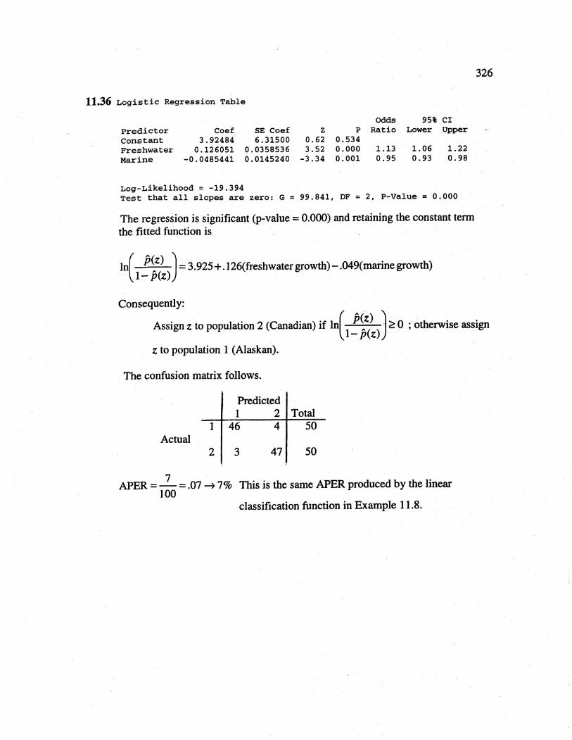
11.36 Logistic Regression Table

Odds 95% CIPredictor Coef SE Coef Z P Ratio Lower UpperConstant 3.92484 6.31500 0.62 0.534Freshwater 0.126051 0.0358536 3.52 0.000 1.13 1. 06 1.22Marine -0.0485441 0.0145240 -3.34 0.001 0.95 0.93 0.98

Log-Likelihood = -19.394Test that all slopes are zero: G = 99.841, OF = 2, P-Value = 0.000

The regression is significant (p-value = 0.000) and retaining the constant termthe fitted function is

In( p~z) ) = 3.925+.126(freshwater growth)-.049(marinegrowth)1- p(z)

Consequently:

Assign z to population 2 (Canadian) if in( p~z) ). ~ 0 ; otherwise assign1- p(z)

z to population 1 (Alaskan).

The confusion matrix follows.

Predicted1 2 Total

1 46 4 50Actual

2 3 47 50

7APER = - = .07 ~ 7% This is the same APER produced by the linear

100classification function in Example 11.8.