m MÜVmmT 01 WATMI in PLANTS

by

Hugh Robert Rovee

A thesis presented for the degree of Doctor of Philosophy

in theEacnlty of Science of the Ihiversity of London

Eebruary 1971

Physics Department Rothamsted Experimental Station

Harpenden Herts

ProQuest Number: 10107286

All rights reserved

INF0RMATION TO ALL USERS The quality of this reproduction is dependent upon the quality of the copy submitted.

In the unlikely event that the author did not send a complete manuscript and there are missing pages, these will be noted. Also, if material had to be removed

a note will indicate the deletion.

uest.

ProQuest 10107286

Published by ProQuest LLC(2016). Copyright of the Dissertation is held by the Author.

All rights reserved.This work is protected against unauthorized copying under Title 17, United States Code

Microform Edition © ProQuest LLC.

ProQuest LLC 789 East Eisenhower Parkway

P.Q. Box 1346 Ann Arbor, MI 48106-1346

ABSTRACT

Sections 2 and 3 of this thesis describe respectively the con­struction and testing of a 30 channel automatic Peltier psychrometer yHiieh records on a printed paper roll. It was shown that with the Peltier type of psychrometer errors caused either by a sample geometry other than that used during the calibration, or by the diffusive re­sistance of the sample can be eliminated by reducing the Peltier cooling time, and the reading time below a critical value. There was reasonable agreement between the theoretically and the practically determined estimates of the critical cooling time. When short cooling times are used however contamination of the thermocouple junction by osmotica is liable to cause a more serious error than when longer times are used. The size of these errors was not sufficient to account for the finding of other workers that leaf water potential measurements are almost constant over large range of transpiration rates.

Equipment for the simultaneous measurement of water uptake, trans­piration and plant turgidity of plants growing in nutrient solution was constructed (section 4) and used (section 3) to examine the movement of water through bean plants exhibiting cyclic variations in transpiration.The hypothesis that such variations in transpiration were caused by a delay in the response of the stomata to a change in the leaf water pot­ential was examined with the aid of a simple mathematical model. Ihe behaviour of the model was similar to that of the plants. The implications of the differences between the two are discussed.

3ACKNÜWLEDGmmrS

Sincere thaniis are extended to the following:-Dr. il.L. Penman for the opportunity to study in the

Physics Department, and for his help and encouragement.To all members of the Riysics Department foi a variety

of reasons, particularly Brian Legg for his assistance with computer programming.

The Director and Mr. Winter of the National Vegetable Research Station for the use of station facilities.

)irs Lyn ilobbs, Mrs Mary Crowther and my father for typing the script.

The Ministry of Agriculture for the I*ostgraduate Student­ship which supported this research.

4

CONTENTS

Section 1 OENEBAL INTRODUCTION1.1 Water potential - the concept1.2 Water transport in plants as a

catenary process

Section 2 A TïïTY-CUANNEL DIGITAL BECCiRDEa JTOB THEBMOCOÜPLE PSYCHROMETEBS

2.1 Introduction2.2 Description of equipment2.3 Aspects of performance

Section 3 SOME ASPECTS OP THE DESIGN AND USB OF SPANNED THERMOCOUPLE PSYCHROMETEBS

3.1 Introduction3#2 Theoretical estimate of critical

cooling time3.3 Experiments using short cooling times3.4 A method of determining the amount of

water condensed by the thermocouple junction

3.3 Contamination of the thermocouple junction3.6 Vapour equilibration3.7 Experimental technique

Page

14

16

202230

3643

46

53657376

Section 4 TUE SIMULTANEOUS MEASUREMENT OF TBANSPIEATION AND WATER UPTAiiE BY A PLANT GROWING IN NUTRIENT SOLUTION

4.1 Introduction4.2 The oxygen requirements of the root system4.3 The aerated po tome ter4.4 The transpiration balance

5Page

77798388

95

Section 5 CYCLIC VARIATIONS IN THE TRANSPIRATIONTURGIDITY AND WATER UPTAEE Ui FIELD BEANS

5.1 Materials and Methods5.2 Estimation of leaf water potential5.3 Induction of cycling5.4 Leaf temperature and the calculation

of diffusive resistances5.5 The relationship between plant turgidity,

transpiration and water uptake5.6 The calculation of plant resistance5.7 The calculation of plant capacitance

106108114

5.8 Discussion

Section 6 C.S.M.P. MODEL OF CYCLIC VARIATIONS IN TRANSPIRATION

1186.1 Introduction6.2 The model - a fundamental hypothesis

7LIST OF FIGURES

Figure Page2.1 Block diagram of fifty-channel digital recorder 232.2 Optical grids used in galvanometer digitizer 252.3 Galvanometer digitizer circuit 252.4 Diagram showing setting of cams on programme timer 312.5 Calibration of galvanometer digitizer 312.6 Decline in output of thermocouples for samples of

various water potentials 34

2.7 Water release curves for two soils 34

3.1 Calibration curves of a prototype thermocouple unitfor two sanyple geometries 38

3.2 Saoule geometries used in the eaq eriment shown infig. 3.1 38

3.3 Effect of sample geometry on the thermocouple output at various cooling times. Sample 0.05molal NaCl. 51

3.4 Effect of sample geometry on thermocouple outputat various cooling times. Sample 0.25 molal NaCl 51

3.5 Integrated output of thermocouple for variouscooling times 54

3.6 Circuit used to introduce an A.C. component intothe Peltier 'cooling' current 56

3.7 Initial output of thermocouple for various coolingcurrents 58

6-

Page

6.3 The plant6.4 Estimation of diffusive resistances6.5 The relationship between guard cell

water potential and stomatal resistance 6*6 Transpiration and the energy balance at

the leaf surface 1^76.7 The C.S.M.P. method of calculation 1^96.8 Results and discussion

Page3.8 Integrated output of thermocouple for various cooling

currents 583*9 Calculated thenDOCoiq>le teaqxerature for various cooling

currents 643.10 Outputs from two thermocouples for various cooling

times 663.11 Integrated output for normal (No 12) and contaminated

(No 7) thermoootq>les for various cooling currents 683.12 Graphs showing negative outputs from thermocoiqples,

after passing 20 mA A.C. for 30 seconds. 683.13 Graphs of initial thermocouple output against amount of

water condensed on junction for normal (No 12) and contaminated (No 7) junctions 72

3.14 Effect of various treatments on equilibration time 744.1 IVinciple of the method for the simultaneous measurement

of transpiration and water uptake 784.2 The effect on transpiration of stopping aeration 804.3 The apparent change in nutrient solution oxygen con­

centration on stopping aeration of the nutrientsolution 82

4.4 Change in nutrient solution oxygen concentrationcaused by the substitution of oxygen free nitrogen for air 82

4.3 Change in oxygen concentration in nutrient solutionafter stopping aeration 84

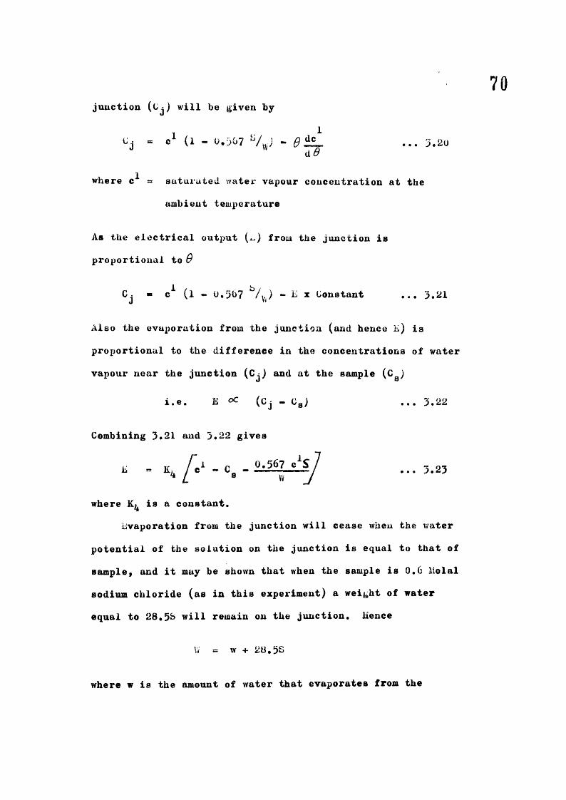
Page4*6 Diagram of aerated potometer 854.7 Diagram of the transpiration balance 904.8 Diagram of the ball bearing dropper 945.1 Graph showing the increase in the average %/eight

of 10 bean leaflets due to water uptake 995.2 Graph showing the relationship between leaf water

potential and relative turgidity for bean leaflets 995.5 Graphs illustrating the progressive increase in

the tendency towards a cyclic mode of tmas- piration 101

5«4 Variation in leaflet temperature on each of thesix leaves of a bean plant during cyclic variations in transpiration 103

5.5 Graph of leaf temperature against transpirationrate for a single transpiration 104

5.6 Graphs showing simultaneous measurements of cyclicvariations in average leaf temperature, transpiration, water uptake rate and plant weight. 107

5.7 Graphs showing the relationship between plant weightand transpiration rate, for various plants exhibiting cyclic variations in transpiration. H I

6.1 Diagramatic representation of the plant used in themodel

6.2 The relationship between estimated leaf water potentialand stmaatal resistance. 1^^

10Page

6*3 Equations of model program 1306,4 Comparison of e3q>erimentally determined trans­

piration, water uptake and leaf temperature waveforms with those produced by the model 133

A1 Diagram of automatic potometer 132A2 Diagram of detector used in automatic potometer 133

LIST 01' TABLES

Table

3.1 Table showing the effect of the Beltier coolingtime on the measurement of leaf water potential 49

3.1 Table showing the range of values of measuredplant resistances 113

6.1 List of parameters used in the model 132

12LIST OF PLATES

Plate Page

3.1 Typical examples of thermo Junctions made from50 s.w.g. (0.001* dia.) wire 42

4.1 Aerated potometer4.2 %krt of aerated potometer showing syringe motor,

commutator, syringe and circulating pimp 874.3 Photograph of recorder chart showing response

of the balance to adding and removing a 200 mg weight 92

4.4 General view of transpiration balance &9A1 Simple micro-manipul at or made frœn disposable

hypodermic syringes 137

ti

LIST OF API hMDICBS

Appendix Page

3.1 The manufacture of fine wire thermocouple junctions 1^63.2 The effect of cooling time on the measurement of

leaf water potential 1393.3 The effect of sample geometry on thermocouple out­

put ^^74.1 A simple automatic potometer ^313.1 Calculation of the phase relationship between

transpiration and leaf toaperatwe 154

14SECTION 1

GINEBAL INTRODUCTION

1.1 Water Potential - the Concept

Plant-water relationships have interested botanists and others from at least the time of Aristotle, who considered that the nutrition of a plant was controlled by its soul. A brief account of the history of the science is given by lùramer (1949). In the present century the work of Ursprung, Thoday and Blackman on cell-water relationships lead to the realisation that water movement was not necessarily along gradients of osmotic pressure but rather along gradients of 'absorbing power'. This 'absorbing power' has been given a variety of different names (e.g. suction pressure, suction tension, effective osmotic pressure, turgor deficit and diffusion pressure deficit). Many of these terms were derived from the theory of osmosis.

The introduction of thermodynamics into the study of water relations has led to the use of the tern 'water potential'. Different workers have used different definitions of water potential, one of which may be expressed as the difference between the chemical potential (partial molar Gibbs free energy) of the water in the system under consideration, and that of pure free water at the s«ne temperature. Defined in this way the dimensions are those of energy per mol, which in practice are seldom used. Frequently the dimensions are converted to those of energy per unit volume by dividing by the partial molar volume of water in the system. Noy-Meir and Ginzburg (196?) point out that this quantity is often unknown and instead they use the molar volume of

15water, (at the reference state) in their definition of water pot­ential. The dimensions of energy per unit volume are convenient because they are equivalent to those of a pressure, and water potentials are often quoted in atmospheres, bars, and hydraulic head units (e.g. metres). Alternatively the water potential of water in a system may be defined as the difference between the partial specific Gibbs free energy of the water in the system and that of water at the reference state, with the dimensions of energy per unit mass (Bri^s 196?). Accurate conversions between energy and pressure units are only possible if the specific volume of water, the t«iq>erature and the pressure are accurately known but for many practical purposes the approximate numerical conversions (calculated for standard con­ditions) given by Barrs and Slatyer (1965) are sufficiently precise.In this thesis the dimensions of energy per unit mass (J hg"" and ergs g"^) have been used as recommended by Slatyer and Taylor (I960), and Taylor and Slatyer (1962).

The total water potential of a tissue has sometimes been divided into the components of matric potential (associated with the capillary and absorbtive forces holding water in a porous medium), the osmotic potential, (associated with the presence of solutes) mud the turgor or pressure potential (associated with the bulk hydrostatic pressure of the water). Noy-Meir and Ginzburg (1967) point out that ambiguity may arise if such a division is made because of solute-matrix interactions. For exaoq»le the total water potential of a systwn consisting of an aqueous solution in a porous medium is not necessarily equal to the sum of the osmotic potential of the solution by itself, and the matric

16potential of an equal amount of pure water held in the porous medium. Warr&n-Wilson (196?) in his analysis acknowledges the problm, and arbitrarily assigns the discrepancy to the matric potential.

The many techniques that have been devised to measure water pot­entials and their associated errors are reviewed by Barrs (1968).Some errors specifically associated with the thermocouple psychrometer are considered in section 3 of this thesis.

2.1 Water transport in plants as a catenary process

In a publication with this title, van den Honert (1948) drew attention to the idea of Gradman, that an Ohm's law analogue may be applied to the movement of water from the soil, through the plant to the atmosphere. Thus, (it was suggested), that the value of any component resistance in the water pathway may be measured by dividing the potential difference between the ends of the resistance, by the rate of water flow through the resistance. This analogy has been used by many workers (Tinklin and Weatherley 1966), and is used in this thesis. The assumptions implicit in its use require comment.

firstly it is assumed that there is no 'active * transport of water. Slatyer (196?) concludes that there is little evidence of active water transport in the sense that water is moved against a gradient of water potential. However, active transport of water in the sense that water movement is associated with the movement of ions is known to occur in plants but according to Slatyer such trans­port is unlikely to be of any great importance due to the short- circuiting effect of the normally high permeability pathways along

17which water moves passively. Both forms of active transport are similar in as much as they are both brought about by a source of energy other than that causing the evaporation, and as such would invalidate the Ohm's law analogue.

Secondly it is assumed that the system is isothermal and that the measurements of water potential are carried out at the same tei^erature as the system (Taylor I968). Without isothermal con­ditions water movement in response to temperature gradients may occur. Cowan (1963) concludes that an analysis using the methods of irreversible thermodynamics indicates that the 'active' transport of water due to the coupling of heat or solute movement is unlikely to play an important part in the transpiring plant.

Thirdly the flow of water through the various parts of the soil- plant-atmosphere system may not be proportional to the difference in the total water potential across each part. In the soil for example water flow %/ill be more proportional to the gradients of matric pot­ential rather than gradients of the total water potential (which may include an osmotic component). Similarly the movement of watervapour from the leaf to the atmosphere occurs in response to gr^ients of vapour concentration, rather than water potential. It is therefore not possible to compare directly the relative magnetudes of the re­sistances to the movement of water in the liquid and the vapour phases. What is required is a comparison of the effect on flow of the same relative change in each of these resistances. When this is done (Cowan and Milthorpe 196?) it is apparent that the resistance to liquid flow is unimportant compared with the resistance to vapour flow.

18This fact, together with the large energy requirement for evaporation, enables reliable estimates of the transpiration from well—watered crops to be calculated from meteorological data without any knowledge of the resistance to liquid flow (Penman 1948, 1949 and 1956). lYhen water is not freely available however, the resistance to liquid flow can affect transpiration indirectly via its effect on leaf water pot­ential and stomatal resistance.

The sites of the major components of the resistance to liquid flow depend partly on the environment of the plant. Even %)lants with their roots growing in wet soil have been observed to wilt under conditions of rapid transpiration. This has generally been attributed to the resistance of the roots but there is some evidence to indicate that the resistance of the stem and the leaves may comprise a significant proportion of the total plant resistance (Cowan and Milthorpe 1968).

The contribution to the total resistance to liquid flow made by the soil is uncertain. The models of Gardner (1960) and Cowan (I965) indicate that under many circumstances t ere is a zone of dry soil around each root which presents a high resistance, (the rhizosphere resistance), to the movement of water. This resistance is a consequence of the radial flow of water towards the roots and of the fact that the hydraulic conductivity of the soil decreases rapidly as it dries. The effect is likely to be most important in dry soils when the rate of water uptake per unit length of root is large. However Newman (1969a and b) and Andrews and Newman (1969 ) have pointed out that root densities are typically larger than those used by Cowan and Gardner (i.e. the rate of water uptake per unit length of root is smaller) and consequently

19the rhizosphere resistance may well be smaller than the plant resistance even in soils near the permanent wilting point. The models from which these conclusions are drawn are necessarily simplifications of the real situation. They do not take account of poorly understood factors such as the nature of the contact between the soil particles and the roots, or the transfer of water vapour to tlie root.

Section 2 of this thesis describes the building of an automatic 30 channel t ermocougple psychrmwter, and section 3 describes ex­periments to examine possible sources of error in the measurement of leaf water potential. Equipment for the simultaneous measurement of water uptake and transpiration, which is described in section 4, was used to make the measurements reported in section 3» In section 6 a sinq>le model is described which was used to examine a hypothesis concerning the nature of the cyclic variations in transpiration.

20SECTION 2

A Eim-CilANNEL DIGITAL RECORDM FOR TiiEBMOCQUPLE PSYCiïRÜMETERS

»1 Introduction

Any closed system containing water and air at constant ten^eratore will achieve a state of equilibrium in which the concentration of water in the vapour phase is determined by the free energy of the liquid water. In particular when the water is held in a porous nwdium by capillary forces, or when ions are present in solution, the equilibrium relative humidity is less than unity, and is a measure of the difference in the specific chemical potential of the water, and tliat of pure water at the same tesq erature. This difference is often termed water potential (Spanner 1964). The range of water potential in living plants of agricultural inqxortance is from zero to about -2000 J Eg~^, equivalent to a range of relative humidity of 1.000 - 0.986.

The design of a thermocouple psychrometer to measure these very high humidities was first described by Spanner (1931) who exploited the Peltier effect to cool a small thermo junction below the dew point of the and>ient air in the chamber containing leaf tissue. The junction then formed a wet bulb wWse depression of temperature below the ambient tesqierature, measured with a galvanometer was directly proportional to leaf water potential. The instrument was first calibrated by using various solutions of sodium chloride with known water potei^tials (Rob­inson and Stokes 1939)

Many variants of this system were subsequently developed. Richards and Ogata (1958) used a droplet psychrometer in which the junction was wetted manually before being sealed into the psychrometer chamber, so

21dispensing with the need for Peltier cooling of the junction* Conq arisons between the Richards and Ogata, and the Spanner types of psychrometer have been made by Barrs (1965), Zollinger et al (1963), and Campbell et al (1966)* The isopiestic technique (Boyer and Ibiipling 1965, Boyer 1966) is a variation of the droplet psychrometer in which salt solutions of known water potential are used on the junction instead of pure water, uater either evaporates from the junction (producing a positive output), or condenses on to the junction (producing a negative output), depending on the difference in water potential between the junction solution and the sample. The water potential of the junction solution that would be in equilibrium with the sanq)le (i.e. produce zero output), can be deter­mined by interpolation. The advantage claimed for this null-point method is that it eliminates any error that would be caused by the diffusive resistance of the sample. IMfortunately the technique is more time consianing, and does not as readily lend itself to automatic control, as does the Spanner method.

Slightly modified forms of the Spanner psychrometer have been used by Monteith and Owen (1958) to measure the water potential of soil sanq}les, and Waister (I965 and 1965) to measure the water potential of leaf samples. Various attenqits have been made to measure leaf water potentials in situ (Lambert and van Schilfgaarde 1964, Lang and Barrs 1965# Boyer 1968, Hoffman and Splinter 1968, Rawlins et al I968), but the need for precise tmoperature contool may limit the usefulness of this techniqw. In situ measurements of soil water potential however are probably easier to make and such methods have been described by Rawlins and Balton (I967),Hoffman and Splinter (1968), Lang (1968), and Rawlins et al (1968).

22The variability of soil and plant material make it difficult to

obtain a representative mean value of water potential without replication.In some systems ten or twelve chambers are selected manually with a thermocouple switch; handling a large number of samples, however, becwnes very tedious. Lang and Trickett (1965) described an automatic system recording the output from four chambers on a peak voltmeter but many more channels are often needed. The apparatus to be described here has been reported elsewhere (Bowse and Monteith 1969)# It accept» the input from 50 Spanner type thermocouples and prints the output from channels selected at will. Similar equipment has been described by Cox (1970 a and b) and Barrs (1969) has described an automatic 25 channel system for use with droplet psychrometer s.

The accuracy with which the water potential of a sample can be measured depends both on the performance of the thermocoiq>le chamber, and on the electrical measuring and recording system. The theory of the design of thermocouple chambers has been considered by other workers (Bowlins 1966, Dalton and Bawl ins 1968, Peek 1968 and I969) and is also considered in section 3# Practical details on their manufacture are given by Merrill I968. Only the performance of the measuring and re­cording system will be examined in this section.

2.2 Description of equipment(a) General description

Tig. 2.1 is a block diagram of the whole system. In brief, voltages from each thermocouple are fed in sequence to a mirror galvanometer.Movement of the galvanometer spot is arranged to produce intermittent illumination of a bank of photoresistive cells, the changes in cell resistance being converted into elecin ic pulses. After amplification

23

Galvanometer

tThermocouplesignal

1Galvanometerrelay

Peltiercoolingcurrent

MotorThermocouple

Programme timer

I (Digitizer and llcounter drive M c ircu it

PulsedsignalSignal

;P r i n t ^ Printing

counterSpace ^

Channel selector

S

Thermocoupleinputs

Channel identification

Fig, 2,1 Block diagram of fifty-channel digital recorder

and shaping, the pulses are counted for a fixed interval of time and the number accumulated, proportional to the galvanometer deflection during the interval, is printed on a paper roll. Two numbers are printed for each channel — a 'zero* reading before passing current to cool the thermocouple and a 'signal* proportional to the wet-bulb de­pression after the cooling current is switched off. Timing of the cooling current, commands to the printer and other sequential operations are controlled by a prograamie timer which conq>letes one cycle for each channel in 72 s. Other times between 60 and 120 s can be selected if needed. At the end of each cycle, a signal from the timer advances the fifty-channel thermocouple switch either to the next position on the switch, or to the next position previously chosen by the setting of a channel selector.

(b) Digitizer

The galvanometer (Tinsley type 4300 A) has a mirror of approximately1 m focal length, a resistance of $41, and a sensitivity of 83 mm A*^ at1 m. It is mounted in a light-tight wooden box along with a lanqp (4 v,8 w) and a set of cadmiim sulphide photoresistive cells replacing the conventional scale.

Two grids (fig. 2.2) produced by the reduction of a large patternon to photographic film, are arranged to give flashes of light as thespot traverses the line of photocells. One grid (fig. 2.2(a)) is placed in contact with a lens in the lamphouse, and a second grid (fig. 2.2(b)) with identical spacing is mounted immediately in front of the photocells. Several sizes of grid have been used, ranging from 10 to 40 lines per cm. The cells (type 38P3—2, Photain Controls Ltd.)

(a)

Pig. 2.2 Optical grids used in galvanometer digitizer

LDROlgF IOmf

J R l 2 N3709

LDR f

I2v

ACYI7

Pig. 2.3 Galvanometer digitizer circuit

26are 6.2 mm in diameter and are mounted at intervals of 1.3 cm in two rows behind the upper and lower sections of the grid, so that when one row of cells is shaded the other is fully illuminated. Each row has twenty cells in parallel, giving a resistance of more than 200 M ji in total darimess, decreasing to about 200 kjx in the shadow position of the grid and to about 10 kji when fully lit. To minimize differences in their characteristics cells were matched to give an approximately uniform sinusoidal change of resistance as the spot scans the whole length of the grid, about 30 cm. Correct focusing of the spot and alignment of the grids is critical, but is readily achieved by observing the moiré fringes that form when adjustment is needed. In principle, it would be more elegant to use a spherical mirror or some other type of light-gathering device to focus the light passing through the grid on to a single cell, but in practice it was found sing)ler to produce a train of pulses from an array of cells without additional optics.

The two sets of cells in opposition act as a potential divider across the input of a two-stage transistor amplifier (fig. 2.3), an arrangement minimizing the dependence of signal an^litude on the intensity of light reflected froa the galvanœaeter. The amplifier produces a train of square pulses from a reed relay ( l i l A ) which is fed to the counter drive circuit. The pull-in current of this type of relay is about twice the drop-out current, so that the circuit does not generate spurious counts Tdien the galvanmaeter spot is disturbed by ordinary vibration. (A con­ventional Schmitt trigger circuit was abandoned because it suffered from this defect.) As the frequency of noise from vibration is higher than

27the maximum signal frequency of about 30 Hz, further protection against spurious counts was achieved by selecting the condenser in parallel with the reed coil (fig. 2.3), to prevent the reed operating above this limit. This condenser also prevents the reed from operating above 30 Hz when the galvanometer spot returns to zero.

c) Counter and drive circuit

Pulses from the reed relay are counted on a printing electrical impulse counter (English Numbering Machines, Series 481) modified by the makers to count 24 v d.c. pulses. The drive circuit for the counter is a modification of that given by the manufacturers for the series 482 counter. The reed relay KLA is coupled to the circuit by condensers which limit the pulse length, and so prevent accidental over-dissipation in the counter coil. A simple divide-by-two device is incorporated in the drive circuit, which enables the galvanometer current to be doubled without exceeding the maximum counting rate of the counter.

d) Zero bias and standard signal circuits

When the psychrometer is used to measure the water potential of leaves, respiration of the tissue can release enough heat to give a small voltage of opposite sign to the output after cooling (Barrs 1965). As the digitizer does not discriminate between positive and negative signals, a small bias of about 0.1^ A is injected into the galvanometer circuit, to ensure that the light spot always moves in the same direction.

At the start of each cycle the galvanometer is connected across a thermocouple in series with a biasing resistance of about 0.5-0. and the

§s

light spot moves about 0.8 cm, producing about 8 (or 16) pulses that are counted and printed. This is the zero reading. The thermocouple is then disconnected from the galvanometer by a double—pole relay with gold-flashed contacts (Siemens type 1^3154/D0720/C412) which is immersed in paraffin oil to minimize thermal voltages. The Peltier cooling current from a Zener stabilized source, is passed through the thermocouple junction for a fixed interval of time, by the closure of no. 6 contacts on the programme timer, cooling it below the dew point of the air in the chamber. Acting now as a non-ventilated wet bulb, the junction is reconnected to the galvanometer and after a further interval, the counter prints a mmber of pulses proportional to the subsequent displacement of the spot. The sequence is then repeated for the next channel selected.

e) Main thermocouple switch and prograiume timer

The main thermocouple switch (CROPICO type SF2/P/ IB) has three poles with fifty positions and is driven by a synchronous electric motor. Two poles switch the thermocouples and the third is wired to a peg board to provide access to selected channels, as described later. When the motor runs continuously, the switch rests on each set of poles for about 3 s, held by a detent mechanism, while a spring in the drive to the switch rotor is wound up. When the spring is fully would the switch begins to inch forward for about 1 s, before jumping to the next position. Bower is supplied to the motor of the thermocouple switch either (i) by closure of the no. 1 contacts on the programme timer or (ii) by closure of a para­llel auxiliary switch fitted to the detent maehanism. The motor is started by a pulse about 2 s long through the programme timer (i), which moves the switch to its next position, thereby closing the contacts of

29the auxiliary switch (ii). This closure maintains power to the motor which winds the spring of the drive mechanism. The switch then begins slowly to move forward towards the next position, but this movement opens the auxiliary contacts and stops the motor, thus ensuring that rotation of the thermocouple switch is always in phase with the programme timer. second auxiliary switch closes briefly after the output from channel 30 hms been printed and causes the printer to produce a row of zeros identi­fying channel 1.

The programme timer (Londex Botaset Adjustable Can Timer) has twelve adjustable cams on a motorised cam shaft lAich, depending on the drive gear assembly, completes one revolution in either 60, 72, 90 or 120 s.The synchronous motor of the timer is supplied with power through the normally closed contacts of a relay. The coil of this relay is in series with the appropriate contacts of the pegboard. Which are selected by the third pole of the thermocouple switch.

Suppose the main switch is about to move from channel 3 to channel 6, and that channels 6, 7 and 8 have pegs inserted in the appropriate holes of the pegboard, to prevent them from being read. As the thermocouple switch begins to inch forward, the third pole completes a circuit pulling in the rei«y which stops the programme timer. With the timer stopped in this position, no. 1 contacts are closed and, because the thermocouple switch contacts are make-before-break, the relay remains energized between successive blank channels. The switch rotates until channel 9 is reached, when the pegboard circuit is broken, releasing the relay and allowing the timer to start a new cycle.

30A typical prograime can be followed on fig. 2.4, where one revolution

of the camshaft corresponds to sixty graduation marks on a setting wheel at the end of the camshaft. In this example, the camshaft revolves once in 72 s, so each graduation corresponds to 1.2 s. Starting from graduation 9*5* no. 4 contacts connect the counter to the digitizer, and graduation later no. 2 contacts operate the galvanometer relay which connects the galvanometer to the thermocouple for the zero reading. Counting is stopped at graduation 26, and the galvanometer disconnected graduation later. The number of counts recorded is printed (contact no. 8) during the passing of the cooling current (graduations 27-43), which is switched by contacts no. 6. The second signal is recorded in a similar manner to the zero signal using contacts no. 3 to switch the pulses and no. 3 to operate the galvanometer relay. The accumulated total is printed (contact no. 7) immediately above the zero count. At the same time the main switch is driven forward by the closure of contacts no. 1. If the next channel is to be read, the switch will dwell on the next position, while the cycle described above repeats itself. Conversely, if the next channel is to be omitted, a pin is placed in the pegboard so that the programme timer stops just before graduation 2. The main switch then moves forward to the next selected channel, as previously described.

To improve legibility, the closure of contacts no. 9 produces a space on the paper ribbon between the pair of figures for each channel.

.3 Aspects of performance i) Sensitivity and linearity

The resistance of the thermocouples is much smaller than the critical damping resistance of the galvanometer, which consequently has a very slow

31

Cam no.Graduations on setting wheel

0 10 20 30 40 50 60T r 1 r

A4_

5_

7

10

Thermocouple switch

Galvanometer relay RLB

Switching of pulsed signal into counterCooling current

Print command

Spacing of figures on roll Standard signal________

Fig. 2,4 Diagram showing setting of cams on programmetimer

200

Ï 100-

200 5Current in galvanometer (#1* )

Fig. 2.5 Calibration of galvanometer digitizer

32respcmse tinae. Ftdl deflection of the galvanometer spot is obtained about one minute after switching into a steady signal. Mg. 2.5 is a plot of the number of counts produced by the full deflection of the galvanometer spot for various known currents. However, the deflection is normally measured after a fixed period of less than 1 min. lor a measuring time of 20 s (as shown in the example in fig. 2.4) 90^ of the full deflection is obtained, without affecting the linearity of the calibration.

The experimental points in fig. 2.5 are all within count of the fitted line. Thermocouple outputs are measured as the difference between a "zero* and a * final* reading and hence might be expected to have an error of jd count, and in fact the calibration curves of the better thermocouple chambers pass within 1 count of the experimental points.The stability of the galvanometer was such that the standard signal was always within hkI count of its average value of 150 over a period of several months.

The internal resistance of the galvanometer is 5^» and the average external resistance is about 2jl, giving a total circuit resistance of

ÂQ accuracy to count (i.e. +0.013 A) will thus be equivalentto +90 nv, or 5 uv on the x2 range. The precision of the system (equivalent to one digit) is thus approximately .0007 degC or 0.007^ in relative humidity at 25*0 or 10 J kg“ (l metre) in water potential.

») Mequency of cyclingA major advantage of automatic recording is the ability to read

selected channels at regular fixed intervals. By oonyaring the printed outputs for successive cycles it is possible to see at a glance when

03equilibrium is reached. If the chambers are read too frequently, however, an error will occur because water condensed on the thermocouples does not have time to evaporate between successive readings. Water remaining on the junction produces a spurious "zero* reading but the subsequent * signal * stays constant.

The maximum frequency of cycling for any type of thermocouplechamber must be determined experimentally, as it will depend on variousfactors. Mg. 2.6 shows that the output from the cooled couples decreasesafter stopping the cooling, at a rate depending on water potential. For

—1example, at -2743 J. kg the wet bulb dries conq>letely in 100 s, but is still slightly wet after 400 s at -461 J. kg** .

) Experimental results

Water release curves were determined for two soils supplied by Dr Lovett of the Uiiversity College of North Wales. The soils were prepared by filling glass columns with 1-2 cm crumbs and then slowly wetting the soil over a period of several imeks. % e columns were allotred to drain and samples of wet soil were placed in the psychrometer chambers. !Rie different soil water contents were obtained by leaving the chambers exposed to the air for various times (0-7 days) before they were put on to the psychrometer.

Mg. 2.7 shows the relation between potential and water content determined with the psychrometer system. Equilibration of the soil in the chambers took about one week. During this time, the system needed no attention; it was connected to a tin» clock so that the chambers were read automatically once every 24 h. Despite scatter attributable to small differences in the conçosition of samples, enough points were

34

>*

CL. 912'

Q.

100Time Cs) a fte r stopping

200 300cooling current

400 500H—after

Fig. 2,6 Decline in output of thermocouples for samples of various water potentials

-30'O'cn~3-

-20

« -10 g

LowlandFridd

• •■ • I

10V • • .-I— I— lb— Wm"-

20 30 40Soil water C 7o dry weight)

Fig. 2.7 Water release curves for two soils

35obtained to enable one to distinguish clearly between the characteristic curves from the two soil types» particularly in the range from -1000 to -2000 J. which is critical for plant gro%vth.

When the system was originally designed, the ability to handle large numbers of samples was considered more important than great pre­cision. In practice, the development of a fully automatic multichannel system has been achieved without sacrificing precision. The system could readily be extended to record output on punched tape.

36

bi CTION 3

SüllF ASPbCTS OF TUF ùLolüN ViND UJi. OF Sl*ilNNFiC ïliiîihMOCüüPLL ■PSYCmiOilLTil .S

3.1 IntroductionSome sources of error in the measurement of leaf water

potential were considered in section 1. In this section only those sources of error specifically associated with the Spanner psychrometer will be examined. Although reference is made to the work of A. J. Peck, the experiments described here were carried out before the publication of his two excellent papers (Peck I968 and 1969}. There is good agreement between his calculations and the empirical experiments described below.

Thermocouple psychrometer measurements have been shown to be affected by air pressure, heat of respiration of the sample (Barrs 1964), slicing of the leaf tissue (Manohar 1966b, Barrs and Kramer 1969), secretion of salts by the leaf (Klepper and Barrs 1969), and contamination of the thermocouple chamber by salts (Manohar 1966a). The effect of pressure can be shown to be small, and as the Spanner psychrometer is normally used, a correction is made for the heat of respiration. The effect of slicing the leaf tissue is probably small provided the amount of cut surface is small compared with the area of the sample. The effect

37(ji; secretion may be important, but at the moment it isonly known to ocaxr with the leaves of cotton. Contamination of the thermocouple chumber can ,te minimised by a careful experimental technique.

Other factors which affect psychrometer measurements are the vapour permeability of the sample (ilawlins 1964), variation in the geometry and placement of the sample within the chamber (Lambert and van bchiffgaarde 1969, Manohar 1966a), and the absorption of water vapour on the walls of the chamber (Lambert and van Schiffgaarde 1969). The importance of these three factors is considered in this section. In addition evidence is presented which suggests that the contamination of the thermocouple junction by minute amoujnts < nult. cau produce a spuriously higi> measurement of leaf water potential.

As an example of the size of the error that can occur due to a change in the geometry of the sample, the results of two calibrations of a prototype thermocouple chamber using different sample geometries, are shown in fig. 3.1 *

To explain these results we must consider the sequence of events that occur during the cooling period of the thermocouple junction, after the instant when the Peltier

* Th<h Ktiïnpie geometries used in this experiment are shown in fig. 9.%

200

Without (liter paper'

With filter paperlOO

o O'! 0-4 0-60-2 0-3 05

Molality of Calibrating Solution

Fig. 3»1 Calibration curves of a prototype thermocouple unit for two sample geometries

38

RubberBungs

4 2 thermocouple

Glass Specimen Tubes

cm

Sample

BA

Fig. 3.2 Sample geometries used in the experiment shown in fig. 3.1

39current starts to flow. The junction temperature at first falls rapidly until it reaches the dewpoint temperature of the surrounding atmosphere. Water is initially removed from a small volume of the atmosphere surrounding the junction. As time proceeds the volume of the atmosphere from which water is removed expands, until, after a fixed period of time (to be called the critical cooling time), the edges of this volume reach a source of water vapour (which is usually the sample;.

If the cooling current is continued, a quasi-steady- state is soon established when water moves out of the sample at the same rate at which it is condensed on to the thermocouple junction. A three dimensional gradient of humidity is thus established between the junction and the sample, which is influenced by :-

(a) The equilibrium humidity of the atmosphere before the passage of the cooling current.

(b) The rate of condensation of water on to the junction.

(c) The distance between the junction and the sample (sample geometry).

(d) The resistance (if any) to the movement of water from the sample.

If the cooling period is less than the critical cooling time, the gradient will depend only on factors (a) and (b).

When the cooling current is switched off, there follows a short period (the "critical reading time"), during which the output from the thermocouple may be considered to be entirely dependent on the gradient established during the cooling period. As evaporation from the junction proceeds, the three dimensional gradient of humidity is reversed, and another quasi-steady-state condition is established. The fact that factors (c) and (d) are operative during both the condensing and the evaporating periods, leads to the observation made by Peck (I968), that it should be possible to take readings of water potential that are independent of sample geometry and resistance effects, by measuring the junction temperature during both the evaporating and the condensing periods. Alternatively, readings of water potential that are independent of these effects can be made by using cooling and reading times that are shorter than their critical values.

The term * quasi-steady-state* has been used above because true steady state conditions are never achieved due to the changes in the effective junction size. For some purposes, however, it is permissable to regard these processes as true steady states. Strictly the change in the water potential of the sample due to the change in its water content should also be considered, but this effect can be shown to be negligible (Peek I968).

iireturning to fig. 3.1 ; the thenaocouple outputs shown

represent the deflection of a slowly responding galvanometer 20 seconds after stopping the cooling current. The reading thus obtained depends not only on the initial output, but also on the form of the output decay, and on the damping of the galvanometer. For this reason very little information can be obtained from these results. Further, although a period of 2k hours was allowed for equilibration, it is probable that the absorption of water on the sides of the chamber prevented equilibration and hence contributed to the discrepancy between the curves. Suffice to show that there is a very significant effect of a change in the geometry of the sample, which may be caused partly by the effect of water absorption by the chamber walls as explained below.

From the arguments outlined above it follows that the direct effect of sample resistance and geometry can be reduced by using a smaller thermocouple junction, and thereby decreasing the rate of condensation.

A technique for making thermocouples from 30 s.w.g. (O.OOl inch diameter) wires was devised and is described in Appendix 3.1. Typical examples of the type of junction obtained with this technique are shown in plate 3.1.

4}i

Plate 3»! Typical examples of thermojunctions made

from 50 s.w.g. ( 0.001" dia. ) wire.

ù

3.2 Theoretical estimate of critical coolinn time

During the steady state condensation period, the gradient of water vapour concentration between the junction and the sample means that there is a deficit of water vapour inside the chamber, compared with the amount in the chamber before the cooling was started. If the steady state rate of condensation is known (and assumed to be equal to that during the non-steady state) an estimate of the critical cooling time can be obtained by determining the time it would take for this deficit to be achieved.

Consider the steady state diffusion between two concentric spheres of radii rj and r^ (where rj = radius of junction and r^ = radius of the chamber).

Let the total flow » N g sec~l inwards

hence flux = - ^ g cm** sec"^krrr"

“ - D dcdr

where c is the concentration at r

hence - ÎL •dr 4 TT D r^

N4 ttD

+ const. .... 3.1

For concentration Cq at r » r.

Iq = — / / + const.4 rr ' '

c „ - c . _ Îl/I ^k7T\> r r

'cTotal content « / c 4rTr^ dr

rDeficit *» (c^ - c) 4 dr

r . J

kTTÏ)2L . 4M !L ^ r" dr

N / r 2 _ r ^ 7D /2 3r /

3.2

For r oJ2 _ 2xr /Deficit « N K _ l i

ÏÏ / 2 3N r "6d *

/ai estimate of the critical cooling time can be obtained by calculating the time required for the deficit to be achieved (asBurning the non-steady state flow towards the junction is equal to the steady state flow towards the junction)

I.e. critical deficitflow towards junction

I N , 2 — • — • *cN 6D. o

ÔD. 3.3

as j) « 0*25 cm" sec“ the critical cooling time is 2/ y ^/3 c

45

strictly this method of estimating the critical cooling time will give an answer that is too large because the value of N is likely to be higher during the initial non-steady state condensation period. From considerations of the energy balance of the junction the error involved can be shown to be a function of

8^

where dg « depression of junction temperature below the ambient during the steady state condensation

Qp m dew point temperature of the atmosphere inside the chamber.

46The method is therefore likely to be more accurate for small values of N (i.e. small cooling currents). However, because the sample is a cylinder and not a sphere of the same radius (as has been assumed in the calculation) it is probable that the critical cooling time can be somewhat exceeded without introducing an intolerably large error. Peck (I968) has calculated that when r^ ** 1 cm and rj « 5 x 10“ ©m for two spherical samples of zero and infinite resistance, the difference in the fluxes of water vapour towards the junction would only be Ifj when the cooling time is 3«b seconds. The critical cooling time as calculated above however is 0.66 seconds.

The time taken for the junction temperature to fall from the ambient to dewpoint temperature is not included in the above treatment. It is readily shown by simple calculation that this time is negligible (Peck 1968, Melvin 1969).

3.3 bxperiments usina short cooling timesIn order to test the possibility that sample resistance

(vapour permeability) and geometry effects can be eliminated by using short cooling times, it was necessary to make the following modifications to the automatic psychrometer.(a; The interval between stopping the cooling current, and

switching in the galvanometer was minimised by arranging for the cooling current to be switched off by a reed relay operated by the same cam as the galvanometer relay. The fast response of the reed relay compared

4?

with the galvanometer relay ensured that the cooling current did not pass through the galvanometer.

(b) The 1 r.p.m, programme timer motor was replaced by a 5 r.p.m. motor, and a four position selector switch was added which enabled one of four pre-set cooling times of 0.75» 1.5, 5.0 and 6,0 seconds to be selected. Longer cooling times could be obtained by manually switching off the programme timer for the appropriate interval during the cooling period.

(c) The reading time was reduced to 2 seconds, and because the maximum speed of the counter was about 30 counts per second, the 'full scale' reading of the instrument was consequently reduced to about 60 counts. A further shortening of the reading time would have been advisable, but it would have resulted in too great a loss of precision. The size of the optical grid in the galvanometer digitiser was reduced so that the 'full scale' reading was about 1500 J Kg~i (i.e. about permanent wilting point).Barrs ( 1 9 0 5 has argued that if a psychometer is

calibrated for two cooling times, and if the vapour permeability of the leaf does not affect the measurement of leaf water potential, then separate estimates of leaf water potential made on the same sample by using the different cooling times should not be significantly different. If however the measurement is affected by the leaf vapour permeability, then

the longer cooling time will result in a larger deficit of water vapour inside the chamber, and hence provide a lower (more negative) estimate of leaf water potential.

This argument is not valid if both cooling times are of sufficient duration to produce steady state condensation, as was probable in his experiment. In a series of experiments in which four species were tested at four levels of leaf water potential, Barrs could not detect any significant difference between readings obtained by cooling for 10 and 60 seconds. (Further evidence presented by Barrs in the same publication, however, is not subject to this criticism and supports his view that the vapour permeability of the leaf is not important.)

In the four experiments described below, the psychrometer was first calibrated for cooling times of 0.75» 1.5 and 6.0 seconds, and then used to measure the apparent leaf water potential of leaf samples using these cooling times.

In experiment 3.2 the leaves were removed directly from plants in the greenhouse, while in experiments 3.3» 3.4 and 3.5, the plants were left overnight in the dark with their roots in half-strength nutrient solution containing u, 100 and 200 g 1“ of polyethylene glycol 4000 respectively.Large polythene bags were placed over the plants. Apparently this treatment did not bring the plants into equilibrium with the water potential of their root environment. The results of these experiments are shown in brief in table 3.1 and in more detail in appendix 5.2 In every case there was a

iùpt.Apparent LWP (j Kg~^)

% L.8.D.0.75s 1.5# 6.0s

3.2 -323.4 -318.4 -353.1 15.83.3 -258.0 -267.3 -336.7 23.23.4 -371.7 -379.3 -429.3 23.23.5 —698.8 -733.0 -764.0 21.6

Table 3*1 Table eummariaing the results of four experiments to determine the effect of the Peltier cooling time of the measurement of apparent leaf water potential

49

5(jsignificantiy lower value ol the leaf water potential when measured with a cooling time of 6 seconds compared with that measured with a cooling time of 0.75 seconds.

The results of these experiments were originally interpreted as showing that there is a significant effect of leaf resistance on the measurement of leaf water potential, however subsequent experiments (see later; showed that similar findings could have occurred if the thermocouple junctions became contaminated with salt after they had been calibrated, which would have the effect of reducing the sensitivity of the junction by a larger amount for the shorter cooling times.

As indicated above, for cooling and reading times less than their critical value, the thermocouple outputs should be independent of sample geometry, further, the cooling times at which the outputs start to differ should indicate the critical cooling time. An experiment was carried out in which cooling times of Ü.75, 1.5, 5.0, 6,0, 12,0 and 24 seconds were used with two sample geometries (similar to those shown in fig. 5.2) and at two humidities (figs. 5.5 and 5.4 and appendix 5.5/• When the sample solution was 0.05 Molal sodium chloride, the results were very much as predicted by the theory, Extrapolation of the lines in fig. 5.5 suggest a critical cooling time of about 0.55 seconds, somewhat longer than the calculated value of 0.2 seconds. Further, these results cannot have occurred because of contamination of the junction by salt, as this would have tended to make the lines in fig. 5.5 converge at longer cooling times.

51

14

< Il

X Discs • Cylinders

O O SM olal NaCl

0 75 1-5 3 6 12 24

Cooling lime (secs. log. scale I

Fig. 3.3 Effect of sample geometry on thermocouple output at various cooling times. Sample 0.05 molal NaCl

5 0

5 45

4 0

35

X Discs • C y linde rs

0 25 M olal NaCl

0 7 5 1-5 3 6 12 24

C ooling t im e (secs. log. scale

Fig. 3.4 Effect of sample geometry on thermocouple output at various cooling times. Sample 0.25 molal NaCl

52thou the sample was 0,25 Molal sodium chloride, the

difference between the two geometries was only just significant, and the interaction between the cooling times and the geometries was not significant (fig. 5.4 and appendix 5,3). ihe failure to detect any marked effect of geometry at this humidity may be due to tne fact that the reading time was too long. For example, there will be a reading time, longer than the critical reading time, for which little or no difference can be detected between the two geometries, because the effects of geometry in the condensing and the evaporating periods will cancel each other.

The findings reported above indicate a need for further information about the effects of sample resistance and geometry, however, rather more sophisticated equipment such as a peak voltmeter (hang and fricket 19^5) would be needed to measure the transient output from the thermocouples shortly after the stopping of the cooling current.

In all subsequent measurements of leaf water potential, chambers of 1 cm radius were used in conjunction with a cooling time of 0.75 seconds and a reading time of 2 seconds. The critical cooling time for these chambers calculated as described above was 0.67 seconds. Ihe maximum cooling and reading tiues for this size of chamber according to the criteria suggested by Peck (I9h8) are each 3.6 seconds. It is likely that any error caused by the vapour permeability of the sample was negligible.

533.4 A method of determining the amount of water condensed bv

the thermocouple junction

The aim of these experiments was to estimate the amount of water condensed by the thermocouple {ii) under any ^iven conditions. It was hoped that a discontinuity in the t reiph of IJ against cooling time would provide an estimate of the critical cooling time. Although this aim was not achieved, the results of the experiments are reported here as they throw some light on the behaviour of the thermocouple, particularly as regards the effect of its contamination.

The straight line calibration* of the thermocouple units at high humidities confirm that the electrical output from the thermocouples is proportional to the evaporation rate from the junction. It follows that the integrated output from the thermocouples will be proportional to the amount of water condensed on the junction. This relationship has been noted by other workers (Barrs 1965 X 1 awl ins 1965), and its validity is supported by the finding that the integrated output from the thermocouple is proportional to the duration of the cooling current (fig. 3.5). This proportionality extends up to 30 seconds, lienee we can

* The curvilinear calibrations reported by some workers (Monteith & Owen 1958) arc a consequence of the slow responding galvanometers used to measure the thermocouple output.

54

>3 -

J- lOO3o

TJDcn

c

3

CD

1 o

O

o 1 2 3 4Cooling time ( secs)

Fig. 3.5 Integrated output of thermocouple for various cooling times.Cooling current 5 m.A. D.C.

55write

.... 3.4where = weight of condensed water (g)

A = integrated üutput 4 voi t sec)

A = a constant (g voif"^ sec”^

ihe output from tne thermocouples was amplified (Comark Type 122 microvoltmeter), and recorded on a Kent 0-10 mV chart recorder, ihe integrated output (n) was found by measuring the area under the curve on the recorder chart.

To calculate it was necessary to be able to vary the current causing the Joule heating in the thermocouple wire (ij) independently of the current causing the Peltier cooling (ip). The circuit used to ao this (fig. allowedeither A.C. or A.t. or combinations of ^ .C. and i).C. to be used for the "cooling* current. The equivalent il.C. heating effect of any combination of A.t. and D.Ü. was measured with an indirectly heated thermistor (o.T.C. iype D54), This component consists of a very small wire coil wound around an electrically insulated thermistor bead; the whole being mounted in an evacuated and gettered glass envelope. As a fui'ther precaution against spurious temperature effects the component was placed inside the constant temperature bath.

Calibration was carried out by passing known direct currents through the coil and measuring the resistance of ike thermistor bead. The D.C. component of the 'cooling* current

56

(DXi■P

Opfl•H

Pfl0)ooO haOO P

ao 0)uaa

g Ü

0) bflü ao •H

TS f—(o Ou O

p üa

•Hu

O 0)P •HP"Tj rHd) QJto PL,0

p•H0ü

■HO

VO

,hD

•H

57was measured with a conventional moving coil meter, it having, first been established that the meter reading, of a direct current was unaffected by a superimposed alternating current.

With one exception the results from all the units used in this experiment were very similar. Only the results from unit No.12 are shown here, as being typical of the majority.

The initial outputs as measured by the maximum deflection of the recorder pen, for various cooling currents, and a constant cooling time of 30 seconds, are shown in fig. 3.7.The points on the steep part of the curves are not accurate because the transient nature of the output under these conditions means that the response time of the recorder prevented the true maximum from being recorded. For larger cooling currents the change in the junction temperature while the recorder pen was moving was small.

Fig. 3.8 shows the integrated output plotted against for the same thermocouple. It can be seen that more D.C. is required to produce the same amount of condensation when the heating effect of the * cooling* current is maintained at a value equivalent to 5 mA D.C. This extra amount of D.C. is a direct consequence of the Joule heating in the wires.

For the direct-current only curve, an increase in the cooling current above 3 mA causes considerably more water to condense on to the thermocouple, but does not increase the initial output appreciably. This is not the case for the constant Joule heating curve, when an increase in the D.C.

lO

I . - 5mA

Sample 0 -6 M NaCl

Cooling Time 3 0 seconds

0 1 2 3 4

DC ( 'nponent of Cooling Current (mA'

Fig. 3.7 Initial output of thermocouple for various cooling currents

1,000Sample 0 -6 M NaCl

C o o lin g time 3 0 seconds

I - = SmA

542 3O

58

D.C. Component of Cooling Current (mA)

Fig. 3.8 Integrated output of thermocouple for various cooling currents

component beyond 3 mul raises the initial output considerably. This difference may be explained if the maximum initial output is obtained only when condensation occurs on a small length of the thermocouple wires supporting the junction (peck I9C8). The extra Joule heating may depress this condensation and hence the initial output.

An estimate of the value of K (and hence can befound by considering the various components of the energy balance of the junction.

hate of Peltier cooling

Latent heat flow

Sensible heat flow (excluding that from the thermocouple wires)

Pip watts

wattst

U6 watts

Sensible heat flow through wires F Ij^) watts

HencePip

where P

Lt

KALt

lie 5.5

» Peltier coefficient appropriate to the junction m 1,74 + I0"2 volts for chromel-constanton.= Latent heat of vaporisation of water (2448 joules g-1) m duration of steady state cooling period (sec)

H w sensible heat exchange coefficient of junction (watts

0 - depression of junction temperature below ambient (**C)

lor small depressions of temperature of the thermocouple junction ( 6 ) below the ambient temperature it may readily be shown that the flow of sensible heat (excluding that from the ires) is almost directly proportional to 6 ,

Spanner (1951) has shown that provided

j = jjgûC 2 • • • 3.6the temperature at any point on one of the themocouple wires is given by

g , Al sin h0((L -JC) _ ^ cos htXTx J . . . 3 . 7

Ea cos h OC L La A / cos h Of L/

w

wherehaKA

\ m fraction of total heat flow from thermocouplewires coming from appropriate wire

L m length of thermocouple wires (cm)X m distance from junction at which temperature

is 0 (cm)y m appropriate specific electrical resistance (ohm cm)

61E = emissivity of surface of appropriate wire

(watt cm“^a o perimeter of wire (cm)K. = thermal conductivity of the wire material

(watt cm”^A = cross sectional area of wire (cm^)

Equation 3.6 requires that for a chromel constantan thermocouple made from wires of the same thickness the lengths of the chromel and constantan wires should be in the ratio0.953 : 1. The ratio of about 1 : 1 for the thermocouples used in these experiments was considered to be sufficiently near to the theoretical value to enable equation 3.7 to be used.

Putting X » 0 in equation 3.7 (when d will be equal to the junction temperature) gives

AF = + ///KA ha~ ... 3.8ha a/ / tan hO( L

or Xf = 0 Constant + Ij^ Constant ... 3.9

A similar equation for (l - A)F may be obtained for the heat flowing towards the junction from the other wire. Adding these two equations gives

F ■ Kj 0+ ••• 3.10

where and Kg are constants.

62Substituting for F in equation 3*5 gives

Pip . + 11 + Kj0 + Kglj^ ...3.11t

or Pip « -1- + Kylj" ... 3.12

where is a constant.ly and Kg "lay be calculated from equation 3.12 and the results shown in fig. 3.8 by putting » 0 and 9 = the appropriate dewpoint temperature (i.e. incipient condensation) when it was found that ly » 37.4 x 10“ and Kg « 1.18 .

The relationship between and Q for a given humidity may be calculated from the equation for diffusion between concentric spheres (Kawlins I963)

H - l l Z f (C3 - c p ... 3.13t dt r^ - rj "

where c-j » c^ - 0 ... 3.14J dû

c = c^a* ... 3.158when c . and c are the vapour concentrations near the J ®

junction and the sample respectively (g cm"^)

c = saturated vapour concentration at 23*C (g cm”-)a^ = activity of solution (relative lowering of v.p.)rj = radius of junction (cm)r^ = radius of chamber (cm)D = diffusion coefficient of water vapour in

air (cm^ sec~\)

63Although this treatment is approximate because the sample

is a cylinder and not a sphere, it can be seen that provided^ the precise magnitude of r^ is unimportant. When

the sample was U,6 Molal NaCl (as in the experiment) we find that

8 - 0.952 H X 10® + 0.553 ... 3.16t

Substituting for & in equation 5.12 yields

. . i .../C / L + Ü.952 % 10® J

and dA ^ 3 ^ ft 3.18dl,P k (L + Kj 0.952 X lo9

Equation 5.17 can only be differentiated when Ij is constant.S is the slope of the line Ij * 5 mA in fig. 3.8. With S - 0.345, K was calculated to be 2.52 x 10"^ from equation 3.18 .

The evaluation of K enables the quantity of water condensed on the junction to be calculated from equation 3.4 . Similarly the junction temperature (fig. 3.9) may be calculated from equation 3.12 by measuring the integrated output.

A surprising feature of fig. 3.9 is the lack of a very distinct change of slope of the curve at the dewpoint temperature when O.C. is used as the cooling current.

64

û.eCl)

X)&)4->oZ3uou

5 mA+ 0 -5

cDC component of cooling current (mA

Eoo Dew point temperature

- 0 5

Fig. 3.9 Calculated thermocouple temperature for various cooling currents. Sample 0.6 molal NaCl

65However this is coiisistojut with the fiauing of A. J. Peck (personal communication), that the dewpoint is difficult to detect when a second thermocouple is attached to the Peltier cooled junction to measure its temperature. Fig.3.9 also suggests that a possible remedy might be to use a mixed A.O. and D.U. cooling current.

3.5 Contamination of the thermocouple .junction

Of the eleven thermocouple units used in these experiments, one (No.7) behaved in a very different manner from the other ten. It was suggested that the anomalous results were caused by a deposit of salt on the thermocouple junction. If this were so one might expect the following symptoms.(a) The initial output from the junction will be depressed,

because the evaporation rate of water from a salt solution on the junction will be less than the evaporation rate of pure water from the junction. Further the depression will be larger when the solution on the junction is more concentrated (i.e. for short cooling times) as is shown in fig. 3.10 .

(b) The output from the junction might be expected to approximate to an exponential decrease, because as evaporation proceeds, the increasing concentration of the salt solution reduces the difference of water

see. 2 sec. 3 sec.

6 0 seconds

4 s e c .

SALT CONTAMINATED THERMOCOUPLE

lO V

r 3 sec

6 0 seco nds

4 sec. 5 sec c o o lin g tim e

NORMAL THERMOCOUPLE No. 12

Fig. 3.10 Outputs from two thermocouples for various cooling times. (Traced from recorder chart)

67potential between the sample anü the junction solution (see fig. 3.10).

(c) if a saturated solution of the salt contaminating the junction has an equilibrium vapour pressure that is lower than ambient vapour pressure in the chamber, then, when the chamber is in equilibrium, the water potential of the junction solution will be the same as that of the sample, A small decrease in the junction temperature will cause condensation to occur before the dew point temperature of the air is reached. That this effect may be occurring with thermocouple No.7 is indicated by the fact that the direct current required to produce an electrical output (i.e. condensation) from junction No,7 was far smaller than for any of the normal thermocouples (see fig. 3.11).

(d) If instead of being cooled, the contaminated junction is heated, water will evaporate from the solution on the junction. This heating may be carried out either by reversing the polarity of the D.C. 'cooling* current, or by using an A.C, 'cooling* current. In either case, when the current is stopped water will be re-absorbed by the solution on the junction and raise its temperature, producing an output of opposite polarity to the normal output. Fig. 3.12 shows the negative outputs obtained from the contaminated and a normal junction after

1,000

500

O 2 4 53

o 7

D.C. Cooling C urrent I mA)

Fig. 3.11 Integrated output for normal (No. 12) and contaminated (No. 7) thermocouples for

various cooling cuirents

68

O ff S ca le

S a lt Contaminated Therm ocouple

No 7

6 0 secsO

q5//Normal Thermocouple

No 12

6 0 secs

Graphs showing negative ou tpu ts fro m thermocouples

a f te r passing 2 0 mA. A.C. fo r 3 0 sacs.(Traced from re co rd e r c h a r t )

Fig. 3.12 Graphs showing negative outputs from thermocouples after passing 20 mA. A.C. for 30 seconds. (Traced from recorder chart)

69puBBing 2Ü uni for 50 seconde. The presence of thesolution on the junction will increase its thermal capacity and this also would have the effect of producing a transient negative output. It is possible that this technique could provide a useful test for contamination of the thermocouples.An approximate figure for the weight of salt (assuming

it to be sodium chloride) on junction No,7 can be obtained from the treatment shown below. The figure is approximate because of a number of assumptions; in particular it is necessary that the electrical output from the contaminated junction (for a given geometry) is a function only of the difference between the concentrations of water vapour at the sample and around the junction, and therefore neglects any effects due to the change in the geometry of the film of condensed water. This assumption is probably less valid for the short cooling times necessary for this experiment, than for longer cooling times.

For a dilute solution of sodium chloride, the lowering of the relative activity is almost directly proportional to the salt concentration and it may readily be shown that

Relative activity = (l - U.567 ... 5.19

where S and W are the weights of salt and water respectively. For a salt solution on a thermocouple junction 6 below the ambient temperature, the vapour concentration near the

junction (Cj) will be given by

üj = c M l - 0.307 ... 5.2Ud 6

where c = saturated water vapour concentration at the ambient temperature

As the electrical output (x.) from the junction is proportional to B

Gj = c^ (l - 0,567 ^I\) “ R X Constant ... 5.21

Also the evaporation from the junction (and hence E) is proportional to the difference in the concentrations of water vapour near the junction (Cj) and at the sample (C^)

i.e. E OC (Cj - Cg) ... 5.22

Combining 5.21 and 5.22 gives

Kt / - C. - - ••• 5-23

where is a constant.Evaporation from the junction will cease when the water

potential of the solution on the junction is equal to that of sample, and it may be shown that when the sample is 0.6 Molalsodium chloride (as in this experiment) a weight of waterequal to 28.5S will remain on the junction. Hence

W = w + 28.5S

where w is the amount of water that evaporates from the

71junction which can be estimated by measuring the integrated output from the thermocouples as described above. Equation 3.23 then becomes

IS - 1 - - K.L ... j.2kw + 28.5Ü ®

which may be solved for E from the data presented in fig.3.13 when the amount of salt (if it were all sodium chloride; contaminating junction No,7 is found to be 4,9 x 1Ü g.The points on fig. 3.13 represent cooling times of 1, 2, 3,4 and 5 seconds, and the line is for equation 3.24 with ü equal to 4,9 x lü"* g. It has been assumed that the relationship between evaporation rate and electrical output is the same for junction No.7 and junction No.12. (This figure was fairly constant for the other thermocouples;.The corresponding points for junction No.12 are shown for comparison. The depression of the initial output (and hence the error associated with the contamination) will obviously be less when the solution on the junction is dilute (i.e. for long cooling times). Thus for junction No.7, for a 1 second cooling time, the initial output will be depressed by about 63^, whereas for the more usual cooling time of 30 seconds, the initial output will be depressed by only about 6ÿ.

Junction No.7 is undoubtedly a very extreme example, but it demonstrates that if short cooling times are used, contamination of the junction is liable to cause much

72

lO

J u n c tio n N o.75

O O 32W e ig h t o f c o n d e n s e d w a te r o n j u n c t io n ( g x IO®

Fig. 3*13 Graph of initial thermocouple output against amount of water condensed on junction for normal (No. 12) and contaminated (No, 7)

junctions

73larger errera than if longer times are used.

5.6 Vapour Louilibration

It is obviously desirable that the necessary vapour equilibration period is made as short as possible in order to minimise the opportunity for a change in the water potential of the sample after it is enclosed in the chamber. Lambert and van bchifigaarde (1965) calculated that neither the rate of heat flow to the sample, nor the diffusion process in the chamber could account for the observed length of the equilibration period, ana concluded that equilibration times were being increased by the absorption of water vapour on to the chamber walls.

fig. 5.14 shows the results of an experiment in which chambers treated with *Kepelcote' (a v/v solution of dimethyldichlorosilane in carbon tetrachloride) were compared with untreated chambers (lines B and A respectively). The points in fig. 5.14 are the averages of ten thermocouples; the same thermocouples being used for both the treated and the untreated chambers. Ulepelcote* apparently reduced the amount of water absorbed b the chamber walls, since the curve levels off more quickly. However it still takes longer than when the sample occupies all the wall space, bimilar experiments using prototype thermocouple chambers constructed

74

jjCLWŒOZ

Oubl6"ΠXI o

o 2

Ol

CL O

— 5 ^ ï

001

o

•H-P

d0•HcSd•HrH•Hg.(U

gcod1cdo>

mdo•Hg>«MO-Pü

cSm

-f

tobD

i_Oo

OOun

O Om 001 O O(siunoD) indjno a|dnoDOUjjaq_L

763.7 Lxuerimentai ïecfaiiiqae

A b a result ol‘ the findings described in this section

(i) New (larger) chambers were constructed.

(ii) Cooling and readin;: times were reduced to Ü.75 and2,0 seconds respectively, h. cooling current of 2,4 niA. was used because it was the smallest current that could be used without too great a loss of sensitivity.

(iii) Chambers were treated with ’Lepelcote* and leafsamples were arranged to cover as much as possible of the chamber walls. It was usually possible to use an entire leaflet and hence avoid any error that might occur through cutting the leaf.

(iv) Chambers were recalibrated immediately before use.

77SECTION 4

TUE SIWUETANEUUS UnASÜlUjMLNT ÜE TilANSfliuiTIüN

AND V>ATEH UrTAlü. Bï A TEaNÏ OUUwINO IN NUTKlENT SOLUTION

4,1 Introduction

The principle of the method used to measure transpiration and water uptake simultaneously is shown in fig. 4,1. If the connection between the root vessel and the potometer is made in such a way that it does not interfere with the operation of the transpiration balance, the transpiration balance then measures the change in the weight of the plant (turgidity), and the transpiration rate over a period of T mine is given by

Trans. Hate (g min“^) - Uptake Hate (g min*“ ) - 2T

where vV is the gain in weight of the plant in grams (which may be negative) over the period of T mine. This arrangement was preferred to the alternative method of mounting the potometer on the balance because it gave a direct measurement of the changes in turgidity of the plant.

The continuous measurement of one minute average values of water uptake for periods lasting many hours using a capillary tube potometer is very tedious. The measurement can readily be automated by the device described in appendix 4,1. However the use of a conventional potometer (manual or

78

p o t o m e t e r

ROOT VESSEL

T R A N S P I R A T I O N

BALANCE

Fig. 4.1 Principle of the method for the simultaneous measurement of transpiration and water uptake

79automatic) necessarily prevents aeration of the nutrient solution, which may affect the water relations of the plant (Uuck, 1967, Slatyer lyhu).

4.2 The oxvaen requirements of the root system

The plants used in these experiments were field beans Vicia faba similar to those described in section 5.

Two series of simple experiments were performed. The first series involved measuring the transpiration of the plants before and after the stopping of aeration. The roots were hermetically sealed into a vessel (?00 cra ) which had a bleed hole at the top to allow air to escape during the aeration period. When aeration was stopped the small air space above the liquid was filled with nutrient solution, and the air bleed hole was sealed. In some experiments there was little or no change in the transpiration rate following the stopping of aeration. Other experiments however (fig. 4.2) indicated that there may have been an increase in the resistance to the movement of water into the root. It is possible that such an increase was responsible for the onset of the cyclic variations in transpiration shown in fig. 4.2a (Barrs and Klepper I968). In another experiment (data not shown) when oxygen-free nitrogen was used to * aerate* the solution, the plant showed marked fluctuations in transpiration and after 2 hours was severely wilted.

2.0co

Ai r o f f( a )

O 62 4 3T i m e ( h r )

80

2 . 0 r

o

S'L. 1.0

oo

(b) A i r o f f

10

Time (hr)

Fig. 4.2 The effect on transpiration of stoppingaeration

81In the second series of experiments an oxygen electrode

was used to measure the fall in the concentration of dissolved oxygen in the nutrient solution following the stopping of aeration. The electrode (Protech type S,M,28/l) consumed a small amount of oxygen and its reading was therefore affected by the ease with which oxygen could diffuse towards the electrode, and hence the degree of stirring of the solution caused by the rising bubbles. This accounts for the apparent sudden fall in oxygen concentration on the stopping of aeration, and its apparent sudden rise on its resumption (fig. 4.3)* A similar effect must occur around the roots of the plant, and stopping aeration may be expected te affect the plant both by allowing a fall in the oxygen concentration in the solution, and increasing the resistance to the movement of oxygen towards the root. This effect does not occur if the air is replaced by oxygen-free nitrogen (fig. 4.4), but if this is done oxygen diffuses from the solution into the nitrogen gas, and is lost from the root vessel. The method cannot therefore be used to measure the amount of oxygen removed by the plant.

In an attempt to eliminate this effect a variable speed magnetic stirrer was used to agitate the solution. Immediately after stopping aeration, the magnetic stirrer was switched on and its speed adjusted so that the reading of the oxygen electrode returned to its original value. The results shown

82

lO O

i j| iO c °

# III

50

A ir o f f

I20 30

T im e (m in»)

80 90 OO 120

Fig. 4.3 The apparent change in nutrient solution oxygen concentration on stopping aeration

lO O

A ir o f fN , on

50N ^ o f f

A ir on

•••

80704 0 50 60302010OTim e (m in»)

Fig. 4.4 Change in nutrient solution oxygen concentration caused by the substitution of

oxygen free nitrogen for air

83in fig. 4,5 were obtained in this v/ay. The rate of depletion of oxygen from the solution increased with the time for which the solution had been in contact with the roots.Oxygen was absorbed by used nutrient solution even when the roots of the plant were removed (fig, 4,5d) whereas fresh nutrient solution apparently absorbed only a small amount of oxygen (fig, 4,5c). This apparent absorption of oxygen may have been caused by a slight change in the speed of the magnetic stirrer. These results suggest that much of the oxygen is removed by micro-organisms in the solution which were found to be present in large numbers.

Some of these experiments showed an apparently enhanced rate of oxygen consumption during periods of rapid transpiration (fig, 4,5 a & b). No attempt was made to confirm this finding. A similar situation has been reported by Hackett and Thiman (1952 and 1953) working with potato tissue. It appears that the concentration of dissolved oxygen was severely depleted within a matter of hours after aeration was stopped and that this depletion is likely to affect the water relations of the plant. It was therefore necessary to make a potometer that would allow aeration of the nutrient solution.

4,3 The Aerated Potometer

A diagram of the aerated potometer is shown in fig.4,6. When a small amount of water was removed from the

84

ücouV?o

O

l O O

o8 0

î Slow tron»pi rat ion

o6 0

IIIèroo O 2 0 4 0

Time (min)

6 0

lO O

Rapid t ra n s p ira t io n

8 0

6 0

2 0 4 0

T im e (m in )

6 0

100

8 0

6 0

T

Fresh n u tr ie n t

s o lu t io n only

(c)

O 20 40Time (min)

60

100

8 0Used nutrient

solution only

6 0

O 20 40Time (min)

60

Fig. 4.5 Change in oxygen concentration in nutrient solution after stopping aeration

y 5

PU M P

ROOTVESSEL

////

//

S Y R I N G E

RESERVOIR

M O T O R

POTOMETERBALANCET R ANSP IR ATIO N

BALALACEI_____

TO RECORDERS

Fig. 4.6 Diagram of aerated potometer

8t)root vessel by the plant, the same quantity of water must be withdrawn from the reservoir. The resulting change in weight of the reservoir was detected by the potometer balance which caused the syringe motor to operate and inject water into the system until the deficit was restored. The amount of water added to the system was recorded by using a printing counter to count the number of pulses produced by a commutator arrangement attached to the syringe drive.One count was equivalent to about 1,8 mg of water.

The nutrient solution in the reservoir was aerated by air saturated with water vapour in order to minimise losses due to evaporation, and the reservoir was covered to prevent water being splashed out by the bubbles. The nutrient solution was circulated by a small pump, which delivered

*5about 130 cm per minute, equivalent to one change of the nutrient solution in the root vessel every 5 minutes. The flexible pipes connecting the root vessel to the potometer passed through the fulcrum of the transpiration balance so that the operation of the transpiration balance was not affected.

The aerated potometer is shown in plate 4.1. A photoelectric shutter attached to the balance pointer was used to switch the syringe motor. The syringe motor, syringe, circulating pump, and commutator are shown in more detail in plate 4.2.

Plate 4.1 Aerated potometer

Plate 4.2 Part of aerated potometer showing syringe motor,

commutator, syringe and circulating pump.

4,4 The Transpiration Balance

A general view of the transpiration balance is shown in plate 4.4. The suspension of this balance was that used by Jennings and Monteith (1954) and was capable of taking loads of up to 20 Kg. The counter-weight and recording mechanisms were re-designed so that the instrument could record losses of weight of up to 100 g. with a precision (depending on the mode of use) of 1-5 mg. The object was to be able to record 24 hours of transpiration from a single plant with sufficient detail to calculate 1 minute averages for selected periods.

Changes in weight occurring on the balance pan (fig. 4.7) were counter-balanced by a chain wheel, driven by a reversible electric motor. The distance between the balance fulcrum and the point of attachment ox the chain to the beam, could be adjusted by a lead screw, so that the effective weight of the chain could be varied between 0 and 2 g. A potentiometer attached to the chainwheel and connected to a chart recorder was used to follow the changes in weight. The direction of rotation of the chainwheel motor was controlled by a shutter on the balance beam, which interrupted a beam of light falling on to a photocell. The photocell was connected, through an amplifier, trigger circuit and relay to the motor, so that depending on the position of the balance beam, the motor always rotated in such a direction as to bring the beam back to its balance position.

89

M

Plate 4.4 Greneral view of transpiration balance

90

JCZ

JZ

o

- c

CL

w£Ox:a

. & i;

L

O 1 O

2

rHC3O•H

-PcS•Hftm

0)«HO

S3Ar

bDip

Ô1The balance beam was allowed to swing freely (its

movement was not limited by stops), with a period which varied between 4 and 6 seconds depending on the loading.The resulting oscillation of the recorder pen produced a narrow band on the chart (plate 4.5)» the centre of which was used when reading the chart.

The arrangement had several advantages, A small stepwise change in weight (less than about 5 mg.) caused the balance to oscillate about a new position, and hence increased the proportion of time spent by the motor rotating in the direction necessary to restore the balance. Larger stepwise changes in weight moved the beaia by an nmount larger than the amplitude of oscillation, so tnat the motor ran continuously in one direction for some time, before starting to reverse direction a ain. The instrument therefore had a proportionating band, the width oT which was a function of the amplitude of oscillation. To obtain a fast response it was necessary to restrict the width of the proportionating band (i.e. restrict the amplitude of oscillation). By using a very sensitive shutter and trigger circuit it was possible to damp the movement of the beam with magnetic damping, sothat it was impossible to detect any visible movement. Inthis condition the balance had a very fast response time which was limited mainly by the speed of the chain wheel motor. Plate 4.5 ia a photograph of a recorder chartshowing the response of the balance to adding and removing

92

03

<D

-P

«HO

<DmÜ -po P3A bOM •HOJ 0)U >

bD bOd a

•HIS oo o

(M02

cd-PP bDc6 d

P3 •Ho >

Od a0) 02

xJ ÎHUo TdÜ02d

bDcS d

•H4-i T lO Td

cdSSA ocd -pUbD 02o O

-po §I—1pLn CdrO

bn

02-Pcd

1—1Pw

a 200 mg, weight.The following arrangement waa used to extend the range

of the balance ao that it could follow losses of weight of up to 100 g. A small peg in the chainwheel actuated a microswitch when the chain was fully wound on to the chain­wheel .

Actuation of this switch (i) Operated a device on the balance beam which dropped

a ball bearing.(ii) Operated an electromagnetic counter.

(iii) Latched the motor relay so that the chain was letdown again irrespective of the position of the balance beam.

Th« motor relay was unlatched by the operation of a second microswitch when the chain was fully let down. The automatic balancing then took over again and a new balance position was obtained. The points of attachment of the ball bearing dropper, and the chain, to the balance beam could be adjusted so that the effective weight of a ball bearing, and the effective weight of the chain was equivalent to either 1 or 0.5 g. The ball bearing dropper (fig. 4.8) held 100 balls so that the range of the balance was extended to either 100 or 50 g.

Iflenc

94

C l

TJ enL.Û L

enC l

gâo

a•HOJ

mQ

dSrO

0)-P

«HO

•Hn00

bC(5

LU

95SECTION 5

CYCLIC VAiaATIONS IN TÜL TK/lNSPIiLLTION. TUmii)ITYUirTAKi, OT Flhh). JiljANti

5,1 Alateriv Ia aud I.;ethods

Field beaus (Vicia faba var. iiaris bead) were grown in nutrient solution in a heated glasshouse. The seeds were surface sterilised by washing for one minute in absolute alcohol, aid then allowed to germinate on moist 'Kimwipe' tissue in the dark at a temperature of 20'L. It was found that running water was essential to produce uniform germination. when the radicles were about 3 cm long, the seeds were Individually supported on foam plastic pads, and transferred to a plastic bowl containing aerated tap water. The tap water was changed for half strength Hoaglands nutrient solution when the first leaves expanded. The nutrient solution was changed every week. Each bowl measured 14” X 14" X 6" and contained nine plants. To avoid damage to the roots when the plants were removed for an experiment, they were later transferred to individual 400 cm^ containers. Artificial lighting (l6 hour day) was supplied during the winter months. When used in an experiment the plants, which were 3 - 5 weeks old with 5 - 8 expanded leaves were transferred to the equipment described in section 4.

96The experiments were carried out in a constant

temperature room at 20'^C.There was no humidity control hut measurements of the

ambient humidity showed that it did not vary greatly during the period of an experiment. Illumination waa obtained from a 1000 watt mercury vapour lamp, and an infra-red filter (4 inches of running water) was used to reduce the heat load on the plant. Metal screens placed between the lamp and the plant were used to reduce the light intensity when required. The maximum light Intensity (between 0,3 and0.7yL/ ) obtainable with this arrangement was 0.25 cals, cm"^ mat a distance of 40 cms from the lamp. No measurements were made of the air circulation around the plant. \Vith noshelter the air currents in the constant temperature roomwere sufficient to cause leaf flutter. To improve the performance of the balance a muslin screen was placed around the plant which reduced the air circulation so that leaf flutter waa just prevented. The air in the constant temperature room was recirculated and hence there was a possibility that the presence of somebody in the room might have caused concentrations of carbon dioxide which were sufficiently high to affect stomatal movements. (Heath 1959, Meidner and Mansfield 1965-) No measurements of carbon dioxide concentrations were made. However because the balance and the aerated potometer recorded automatically it was not usually necessary to spend long periods in the room.

97It was also possible to obtain some air exchange with fresh air from outside.

1efore an experiment the plant was always left overnight in the equipment to ensure satisfactory temperature equilibration of the nutrient solution.

5.2 Estimation of leaf water potential

As explained in section 4, the transpiration balance, when used in conjunction with the aerated potometer, measures changes in the turgidity of the aerial parts of the plant.A change in the water content of the root will only affect this measurement if, when the root absorbs or loses water, its change in volume is not equal to the volume of the water absorbed or lost, although it is probable that this occurs, its effect is almost certainly negligible.

If the relationship between plant turgidity and leaf water potential is determined, it is possible to use the changes in plant turgidity to obtain an estimate of leaf water potential. Ine relationship between leaf water potential and relative turgidity was not determined for an entire plant but only for individual leaves. If, as seems probable, most of tne loss of weight in wilting plants occurs in the leaves, then it is possible to estimate leaf water potential from measurements of plant turgidity (weight). However because no account is taken of any change in the water content of the stem, such measurements' are likely to

98overestimate the deficit (and hence the stress) in the leaves.

.V!uch has been written about the concept of relative turgiuity (jlatyer uud Barrs 1965), and the problems of its measurement. Une of the main difficulties is that leaves (or leaf discs), when placed in contact with water, do not show any definite water saturation weight, lor this reason the uptake of water by wiltou leaves was followed in order to determine a standard procedure for measuring relative turgidity. Figure 5.1 shows the average weight of 10 bean leaflets following the insertion of their bases into slits in water saturated foam rubber. To minimise errors due to infiltration of the intercellular spaces, entire leaflets (as opposed to leaf discs) were used, and only the basal3 - 4 mm were inserted into the rubber. A standard drying procedure was used which involved placing the leaves between4 thicknesses of 'lliuiwipe* tissue and compressing with a 500 g, weight for pO seconds. From figure 5.1 it appears that the majority of the initial uptake was completed by 4 hours (this time was used in subsequent experiments), although a slow uptake continued for some time afterwards.

The relationship between relative turgidity and leaf water potential (measured as described in section 3), is shown in figure 5.2. The wilting was induced by removing the plants from the nutrient solution. Most of the leaves of these plants consisted of only two leaflets ; one leaflet

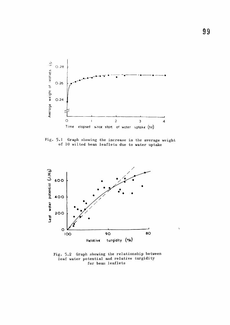
cn0 . 2 8

I/)Vocv

0 .2 6o

icO’ty$ 0 . 2 4

wcnO%<

0 1 2 3T im e elapsed since start of w a te r uptake (h r )

Fig. 5.1 Graph showing the increase in the average weight of 10 wilted bean leaflets due to water uptake

/C7»

V%9B3

too

400

200

O 8090lO O

99

R ela tive tu rg id ity (°A>)

Fig. 5.2 Graph showing the relationship between leaf water potential and relative turgidity

for bean leaflets

100was used for the measurement of relative turgidity, the other for the determination of leaf water potential. The dashed line in figure 5.2 was used to estimate leaf waterputouvi ds from measurements of relative turgidity.

5.3 Induction of cvclinu

Some plants started showing cyclic variations in transpiration spontaneously for no apparent reason; others could be induced to cycle by giving a short (20 minutes) dark break in the middle of a light period. Such induced oscillations were sometimes sustained, but frequently died away after one or two cycles. As has been found by other workers (Skidmore and Stone 1964, Shrler et al 19^5» Barrs and Klepper 1968), oscillations were found to occur in the late afternoon and evening. Plants wnich showed little tendency to oscillate could often be induced to oscillate after being subjected to several hours of bright light.Figure 5.3 a b c show the transpiration and uptake immediately following a dark period of 20 minutes which ended at the times shown. It can be seen that the oscillating tendency increased during the day. Figure 5.3 d shows a portion of the sustained oscillations which occurred spontaneously on the following day, after an 8 hour night. These oscillations continued undamped for at least 6 hours. Reasons why a plant should change from a non oscillating to an oscillating mode of transpiration are considered later.

2 I 30 pm

X X x _ % _ X - X X - x - x - X — X I Q \

X U p ta k e

OmO

Tu O ^ 2 0 3 0 4 0 5 0 7 0 W in u k ^% 2■ 5 . 3 0 p m

(b)# T r a n s p ir a t io n

IQ 2 0 3 0 4 0 SO 6 0 7 0 M inutes

9 . 5 0 p m xX

• X

X Uptake

• T r a n s p i r a t io n

O 7 0 M in u te slO 20 6 03 0 5 04 0o 2

X Uptake « T r a n s p i r a t i o n

O lO 2 0 3 0 4 0 5 0 6 0 7 0 M in u te s

Fig. 5.3 Graphs illustrating the progressive increase in the tendency towards a cyclic mode of transpiration

101

1025.4 Leaf temperature and the calculation of diffusive resistances

Measurements of leaf temperature were ruade to determine whether all the leaves were showing cyclic variations in

transpiration, and if so, whether they were in phase with

each other. The 42 s.w.g. chrouiel-constantan thermocouples

were threaded into the midribs of the leaflets from the

abaxial side. To minimise the effect of conduction along

the wires, the thermocoupleg were threaded so that there was

about 3 mm between the junction and the points at which the wires emerged from the leaf. The reference junction was

placed in the air about 10 cm from the -plant, and shielded

from radiation from the lamp. Tue outputs from the

thermocouples were recorded on a ment 0-1 mV multipoint

recorder.

Fig. 5.4 shows the measured temperatures of one

leaflet on each of the six leaves on a plant. All the

leaves showed cyclic variations in leaf temperature (and

hence transpiration) which were in phase with each other.

The higher mean temperature of the upper leaves (No. 6, 5»

4 and 3j compared with leaves No.l and 2 is probably due to

their greater radiation load.

It may be shown (appendix 5.1) that in this experiment

the heat capacity of the loaf is sufficient to cause the

oscillations in leaf temperature to lag behind the oscillations

in transpiration. Such a lag was demonstrated (fig. 5.5) and

4-2

103

-2

.u" 4-2

c

Ü -2JQÊo +2 o

-2

+ 2

+ 2

-2

4 -2

-2 ©«.* ' .* •.* " »

O lO 2 0 3 0 4 0

T im e (m in )

50 6 0 70

Fig. 5.4 Variation in leaflet temperature of each of the six leaves of a bean plant during cyclic variations

in transpiration

104

r +

T r a n s p i r a t i o nCl

c

£o0.2 0.6 oa

ot r a n s p i r a t i o n V increasing? >

o

transpirationdecliningL -3

Fig. 5.5 Graph of leaf temperature against transpiration rate for a single transpiration cycle.Note that the leaf temperature lags

the transpiration rate

105this f i n d i n g provides further confirmation that the response

time of the transpiration balance was sufficiently fast for

these experiment3,

The measurement of leaf temperature also enables

diffusion resistances to be calculated as shown below. The

total diffusion resistanuu so obtained is the sum of a leaf

diffusion resistance, (stomata! ana cuticular resistances

in parallel), and an aerodynamic or boundary layer resistance.

Total diffusion resistance r^ - " Xa. 5.1

‘..here X and X a the absolute humidities of the water

vapour inside the leaf and in the air (g cm“^), and m is the

transpiration rate sec~^ cm"^,, X can be obtained from

vapour pressure data by

X - X lO"^ g cm*" 5.2'!

where T = temperature ("K,

e vapeur pressure (millibars;

Ihe vapour pressure inside the leaf is taken as the saturated

vapour pressure at leaf temperature.The leaf temperature data were also used to provide a

reliable estimate of the ajiiount of radiation absorbed by the

plant by equating the absorbed radiation with the latent heat

associated with the transpiration rate when the average leaf

106temperature is equal to the ambient temperature,

5.5 The relationships between plant turbidity, transpiration

and water uptake

The changes in plant weight, transpiration, and water

uptake shown in fig. 5.6 were measured on a single plant,

but these data are typical of the majority of the plants

used in this equipment. ihere was usually a steady increase

in the weight of the plant in addition to the oscillations

in plant weight, (in this example it was as much as

50 mg hr~i/. It is probable that this was caused by growth.

This increase has been deducted from the balance reading to

give the "corrected balance reading" shown in fig. 5.6.

Fig. 5.6 shows several important points. Firstly, as

has been noted by Lang et al (1969) the plant weight

(turgidity) is out of phase with its normal (non-cycling)

relationship with transpiration rate, (i.e., when the plant

is turgid the transpiration is slow and vice versa).

Secondly, although the uptake rate lags behind the

transpiration rate as might be expected, the amplitude of

the variations in the uptake are apparently as large as the

amplitude in the variation of transpiration rate. This

might be expected if the transpiration balance was too slow

in responding to the changes in weight of the plant. This

explanation however appears unlikely (see plate 4.5,

section 4), and as no other explanation as to why this

107

II

- Z o °I q| JUiiquiO OJ »AIJC>1»J B);»! *Bw»AV »>1oidn / uonojidsuoji

«3a 'do•H-Pd 03•H -pk dd U> 03ü•H -3r-t P>ü Phdü bJD

u d<P 0) •HO P3ndd dw 03-p d03 d 03a o 03eu •Hp Pd d r4en d dd •H P0) Pha en 'd03en pd d 03o P 0303 dd03 OP> d 03r—1 dd pa d P•H d Pen 03 bJ3P h•HbD a 03fl 03 !5-H P:& po PÆ den 03i—i1—4 PhenÆ oA bod dd dO 03SVO 03m 5

bD dg:•H

O O O( 5 1 6uipo»j wuD|oq P»J3»JJ03

108result might be spurious coulu bo found, it must be accepted

as genuine, Tho finding may be of some significance as it

might be expected that the capacitance of the plant would

damp the uptake amplitude so that it was less than the

transpiration amplitude. This damping is illustrated by

the model described in section 6. No explanation is given

for the similarity in amplitude observed in the experiments.

The transpiration rate and uptake rate will of course

oscillate about the same mean.

5.6 The calculation of plant resistances

Tinklin and beathcrioy (ly6d) define a plant resistance

using the Ohm's lav; analogue

liant resistance £ * VlI - Ya ...... 5.3f

or if y ~ 0 £ = - jgb .... 5.4K f

where y and are the water potentials at the root

surface, and in the leaves, and f is the flow of water

through the resistance. It is necessary to stipulate that

the plant is in equilibrium with a steady transpiration

rate, (when f will be equal to eitner the uptake rate or

the transpiration rate), in order that f has a precise

meaning, equation 5.4 also requires that the leaf may be

considered to be at a single water potential If a

1U9Biguific.nit proportion of tho total plant resistance to the

üiovoment of water is in the leaf, there will be a gradient

of water potential in the leaf, and it is not possible to

apeak of a single leaf water potential. Little is known

about the relative magnitudes of root and leaf resistances

(uowan and diithorpe ijuü;, but it is possible that the

resistance to tue iioveuaent of water in the leaf is not

negligible (Lospisilova 19&9).

riant resistances have been expressed in a variety of

units. For the purposes of the model (sec cion 6), it is

convenient to express in ergs and f in g sec*l, soOthat the units of R are cm" g” sec“ . The units of

atm sec cm“^, used by box (l9bw), and bar h dm", used

by Larrs and hlepper (ipod), are uerived by expressing y

as atm and bars, and f as ciu- sec"” and mg h*" dm""

respectively.

ijsinp the relationships

h, » (from eq. 5.4) 5.5df

y = 0.462 (100 - y) X 10^ ergs gm“^(fig. 5.2; 5.6

y = 100 - lüOD 5.7* f -

dD = - dW 5.8F

110where y

i)

W,,

I

relative turgidity (p;

plant water deficit (g)

turgid weight of leaves (g)

dry weight of leaves (g;

fresh weight of leaves (g;

It may he shown tuat

46,2 X 1Ü 5.9

If most oi resistance to water movement is in the roots

of the plant, \anu most of tne capacitance in the aerial

parts oi t'ac plant;, f will be very nearly equal to the

rate of water uptake b by the roots,

equation 5.V then becomes

du”46,2 X 10

%D

The reason for calculating the plant resistance in

this way is tint the equipment described in section 4

cannot measure directly the water deficit of the plant;

it can only measure changes in the deficit i or fresh

weight).Graphs of W, (the corrected balance reading) against

uptake rate are shown in fig. 5.7. Some of the results

(plants A and D) show a linear relationship between bj, and

5.10

Ill

XPlant A

•\

0 5 0 5

Plan t

0 .30.2 0 . 4 0 . 4 0 . 5 0-6Flocid Turg d Flacid Turgid

0 5 0 . 5Plant D

Plant F

0 . 5 0.6 0 .7

0 . 5P la n t E

P la n t E

0 .70 50 .4 0 6 0 .5 0.6 0.7

C o r r e c t e d balance reading (g .)

Fig. 5.7 Graphs showing the relationship between plant weight (corrected balance reading) and transpiration rate for various plants exhibiting cyclic variations

in transpiration

112uptake rate. With other plants however the rate of water uptake was not directly proportional to Wp, hut showed hysteresis. Several alternative explanations may he put forward to account for this finding, hut there is little evidence to suggest which (if any) is correct. For example it is possible that there was a significant proportion of the plant resistance in the leaves which consequently developed gradients of water potential. The potential difference across the root would therefore he smaller during the drying part of the cycle, and larger during the ahsorhing part of the cycle than was estimated from the measurements of plant weight.This factor in itself should not cause a large error in the measurement of the plant resistance, because if a complete cycle is taken, the errors in each direction will cancel.A second possibility is that relationship between relative turgidity and leaf water potential exhibits hysteresis.(Slatyer I967, Kelsey 1957).

Experiments were carried out on two plants (plants D and £ table 5.1), when half of the leaf area (one leaflet of each pair) had been removed. The object of removing the leaves was to determine if this treatment affected the period of oscillation (which it did not). However the resistance of these plants, as calculated by equation 5.10, was apparently greater than when the entire leaf area was present. Cowan and Milthorpe (l96s) report an experiment of Cox with sunflower in which one of each pair of opposite leaves was removed from

CM lA o 0% (S. ?rH CM r^ tAü

fH lA lA •HCM

.y* o\ 00 C-J rH O * t CM

H

00 ml r»% a e ^

iH V£> 00 o oCMCl

113

i

M

ICM

S R S a ? os OS tAt !» oô o r4 o l l tÀ

i-ilM

R 8 OfH

CM <DrH

V»

CM m rR 2 R

VM3 O iH Ooocô

0000 r \

i VO

o

CM

CM

5 S o»H Co 2 R

Jî cîM vÔ â iH O

S « 3 a §t l o m4 O

S 5 » & aCM ri o o o

U W) lafi ta bfi b6

a

1 1

t tna 3b&

a-P ao ao fek a A« a• iH -pt • •fO taa t>>>« SsS A

m-MoS

K\

00

m

iH

!<a «^ : 1=^0

r \

00

m

iH

CW

g.2 'gaa I

A

| 5

O

m

ÜCM

m

"%

® CM_

« -= « T

1 aa •“

ÎA

E4

114the plant. Cox calculated that the resistance of the leaf was about twice that of the roots plus stem. Unfortunately the interpretation of this type of experiment is difficult because the results may depend on the arrangement of the xylem vessels.

Table 5.1 shows the range of values of the measuredplant resistances. The average resistance of these plants was60 X 10^ atm sec cm"- . Cox (reported by Cowan and Milthorpe1968) found a value of 17.6 x 10^ atm sec cm”^ for sunflowerplants, and Jenson et al (196I) found a value of 14.7 x 10^also for sunflower plants. Some of the difference betweenthese figures and those calculated for the bean plants may beaccounted for by the smaller average size of the bean plants(1.66 g dry weight). The sunflower plants of Cox had anaverage dry weight of 4.0 g (Cox personal communication).If the plant resistances are converted into the units used byBarrs and Klepper (1968), the average value for the resistanceof the bean plants is 0.00307 bar mg” h dm^ which is slightlylower than the values quoted by these workers (0.0041 to0.0053 bar mg“ h dm^j for their low resistance (non cycling)pepper plants. Pepper plants that showed cyclic variations in

—1 2transpiration had resistances from 0.0090 to 0.0161 bar mg h dm .

5.7 The calculation of plant capacitance

The total plant capacitance (assuming it all to reside in the leaves) can be estimated from the turgid weight of the leaves and the relationship between relative turgidity and

115leaf water potential, by analogy with an electrical capacitor, where charge is analogous to the water deficit of the leaf, and electrical potential is analogous to water potential,

i.e. For a Capacitor,Capacitance = Charge_______ ... 5.11

Electrical Potential

and for a plantPlant Capacitance = Water Deficit (i>) ... 5.12

Leaf Water Potential

From equations 5.12, 5.6 and 5.7

% T pPlant Capacitance « _________

0.462 X 10^

The above treatment assumes that there is a linear relationship between relative turgidity and leaf water potential. This assumption can probably be justified at least for small deficits of water (Weatherley and Slatyer 1957» Jarvis and Jarvis 1963, Bhlig and Gardner 1964).

5.8 Discussion

It may be shown by simple calculation that the changes in the transpiration rate must be caused by changes in a water vapour diffusive resistance. The site of such a variable resistance is almost certainly the stomata although it has recently been suggested (Jarvis and Slatyer 1970) that the

116mesophyl ceil walls may provide such a resistance.

The various hypotheses that can be put forward to explain the variations in stomated resistance may be divided into two groups.

(a) The variations in stomated resistance are caused by some factor not directly concerned with the water relations of the plant (e.g. carbon dioxide induced stomata! movements), and the variations in transpiration rate, turgidity and uptake rate are merely a consequence of this. This may be called "water independent" cycling.

(b) The changes in transpiration, turgidity and uptake rate are an integral part of the oscillating mechanism. This may be called "water dependent" cycling.

There is insufficient evidence to state categorically which of the two hypotheses is correct, but such evidence as there is points to a "water dependent" oscillatory mechanism.Most of this evidence is reviewed by Barrs and Klepper (1968) and Lang et al (1969) end will not be repeated here. While it is believed that the oscillations described here are "water dependent" it is not suggested that this applies to all oscillations, liaschke (I965) demonstrated that cyclic variations in stomatal aperture may be attributed solely to fluctuations in the internal carbon dioxide concentration.Barra and Klepper (1968) suggest a possible criterion for

117distinguishing between the two types of cycling is that the period is less than ten minutes when only the internal carbon dioxide concentrations are concerned. Cox (1968) suggests that the oscillations in sunflower are brought about by hydropassive stomatal movements causing the stomata to overshoot. Barrs and Klepper (1968) however consider that hydropassive stomatal movements do not occur in sunflower and 80 in this species at least it may be necessary to look for some other explanation. Â simple model, which does not include hydropassive stomatal movements, and yet produces oscillations similar to those found in the plant, is described in the next section. However it seems certain that where hydropassive stomatal movements do occur they must tend to accentuate the oscillations, and they could be the sole cause of oscillation in some species.

118SECTION 6

C.8.M.P. MODEL OF CYCLIC VARIATIONS IN TRANSPIMTION

6.1 Introduction

An essay on the value of mathematical models is inappropriate here (see de Wit 1969), but a fev remarks are necessary in order to avoid confusion about the objectives of this investigation. Any explanation put forward to account for cyclic variations in transpiration must eventually be judged by two criteria!-

(i) The explanation must be physically realistic(ii) The eaq>lanation must enable the production of sustained

oscillations similar to those found in nature, but it must not make the oscillations inevitable.

We have insufficient information to satisfy completely the first of these criteria; nevertheless the feasibility of various hypotheses can be examined by using a model to see if they satisfy the second.It is not suggested that the system to be described would be accurate for all the deductions that could be made from it.

Electrical analogues have been used by several workers (Meleshchenko and Karmanov 1966, Lang el 1969) to simulate cyclic variations in transpiration. Such analogues suffer from disadvantages. Firstly, it may be shown that while it is possible to use the Ohm's law analogue for either the flow of water in the plant, or the diffusion of water vapour through the stomata, the dimensions of the potentials and resistances in each case are not the same, and a system with both

119liquid and vapour flow cannot be adequately represented by a simple electrical analogue (Philip 1966). lor example, if in our electrical analogue electrical potential is chosen to represent vapour pressure (real or virtual), we find that

(i) Diffusion through the stomata is directly proportional to a difference in vapour pressure

(ii) Passive isothermal movmnent of liquid water is proportional to a difference in water potential which is a non-linear function of vapour pressure.

Another disadvantage of the simple electrical analogue is that it fails to represent the energy balance at the leaf surface and does not, for example, take account of such factors as changes in leaf tmnperature. The model to be described avoids these two problems.

Yet a further disadvantage of the simple electrical analogue (which is shared also by the present model ) is that the sites of resistance and capacitance are separated spatially because they are represented by discrete components. Such a separation may be justifiable when considering the water exchange of a cell vacuole (capacitance) through the cytoplasm and plasmolemma (resistance).Water movement in the cell wall however, should probably be represented by a pathway with continuous resistance and capacitance* It should be possible to modify the model to include such pathways, but the lack of quantitative information does not allow this refinement at the present

time.

120In building the model an attempt has been made to follow two

principles. Firstly, lAenever possible measured values of parameters were used which were based on the results from a single plant. The use of arithmetic mean values was not thought desirable.Secondly, when deciding between two alternative forms of the model, the alternative which involved the least number of assumptions was chosen. Fbr exanqile, it is probably justifiable to divide the total plant resistance into its component parts of root, stem and leaves. Such a division was not made because there was little information on the probable resistances of the ccssponent parts, whereas there ims a good estimate of the total plant resistance. The operation of this principle resulted in a crWe but singple model.

6.2 The model - a fundamental hypothesis

A diagrasmatic representation of part of the model is shown in fig. 6.1. Electrical symbols have been used for convenience and in this example the analogy with electrical exponents is conplete.

It was shown in section 5 that the stcmiatal resistance was out of phase with its normal relationship with the leaf water content.The fundamental hypothesis which is tested by this m>del is that this phase difference is caused by the pathway taken by water vhen it moves between the sites of evaporation inside the leaf and the stomatal guard cells. It is supposed that this pathway (which is closed at the guard cell end) presents a resistance to the move­ment of water and also has the capacity to absorb water, such that if there is a step-wise change in the water potential at the sites

121

Stomata

Trans R2 R2 R2V2 V3 V4 Guard

" cell'

C2 C2 C2 -

Uptake U • Stomatal Pathway

V = water potential I = water flow R= Resistance

d V I / d t - - 1 2 / C l

d V 2 /d t - ( I 3 - I 4 ) / C 2

dV3/dt = ( I 4 - I 5 ) / C 2

d V 4 / d t = I 5 / C 2

Uptake (U) = 11 + 1 3 - 1 2

Change in plant weight (Q) = ( C l x v i ) + C 2 ( V 2 + V3 + V4)

12 = V I /R I + 1 3 + 11

13 =(V I - V 2 ) / R 2

14 = ( V 2 - V 3 ) / R 2

15 = (V3 - V4) /R2

Fig, 6.1 Diagramatic representation of the plant used in the model

122of evaporation (V1 fig. 6.1), an interval of time elapses before the full effect of this change is seen on the guard cell water potential (V4). This pathway is represented by the three capacitances 02 shown in fig. 6.1. The components of the pathway have no individual significance. For convenience only three resistance/capacitance units were used, as this was the smallest number that would produce the necessary phase lag required by the hypothesis. No measurements of the capacitance of this pathway could be made. However, provided the capacitance is small (a value of 0.1 x 10"^g imT^sec^ per unit was used) compared with the capacitance of the plant 8.0 X 10~®g cm ' sec ) it will be seen that its precise value is of little importance.

Early experiments with the model showed that the period of oscillation was dependent on the product of the resistance and the capacitance in the pathway. It therefore follows as a corollary of the hypothesis that if the period of oscillation is to be correct the fixing of the capacitance of the pathway automatically fixes the resistance of the pathway.

6.3 The plant

The total plant resistance and capacitance were estimated as described in section 3 and are represented in fig. 6.1 by fil and Cl respectively. The configuration in fig. 6.1 represents the situation when water flows through a pure resistance (say the roots) to a site of pure capacitance (say the leaves). This is certainly not the true situation in the plant, but it may represent a

123reasonable approximation. For example, the capacitance of the plant must include both the capacitance of the cell vacuole and that of the cell wall (Weatherley I963). There will be a resistance to the movement of water between these two sites, hence the total plant capacitance cannot strictly be represented by a single capacitance unit. However, Cowan and Milthorpe (1968) calculated from the work of Philip (1958 a,bckc 1966) that half-times of the order of seconds are to be expected for the equilibration of water potential between cell walls and the cell protoplasm. If this is true, little error will result from representing the sum of these capacitances by a single component.

6.4 Estimation of diffusive resistances

The total diffusive resistance, r^, was calculated as described in section 3, and is the sum of a leaf diffusion resistance r^ (stomatal resistance r^ and cuticular resistance r^ in parallel) and an aerodynamic resistance r^.

The cutiular resistance, which was not measured, is unlikelyto be important in these circumstances because it only affects thetranspiration rate Wien the stomatal resistance is high. For

—1ecmq)leteness a typical value of 33 sec cm was included.The aerodynamic resistance was estimated by assuming it to be

equal to the aerodynamic resistance to the transfer of sensible heat between the leaf and the environment. The sensible heat transfer is given by the equations

124H - t(,T' ...6.1

and y? G T*II- . . . 6.2

awhere

oCs • sensible heat transfer coefficient (cal cm sec""T* - difference in temperature between the leaf and the

environment (®C)- density of air (g cm"" )

Cp ■ specific heat of air at constant pressure (cal g**0(3 may be calculated from

" 0((sensible) « K(total) - o((l.w. radiant) ••• 6.3oC(total) is estimated as described below (equation 6.12), and

OC (l.w. radiant) can be estimated from the Stefen-Boltsanan equation if it is assumed that the leaf acts as a black body to long-wave radiation.

6.5 The relationship between guard cell water potential and stomatal resistance

This relationship is not easy to measure directly because of the difficulty of measuring the water potential of the guard cells. It might have been possible to determine the relationship from steady state (non-cycling) wwwements of stomatal resistance and leaf water potential by assuming that in the steady state the guard cell water potential was equal to the leaf water potential.

125However, this approach assumes that the relationship is the same in both the steady state and the cycling type of transpiration* %

assuming the existence of the hypothetical stomatal pathway a 'relation­ship* can be obtained. However although this method was used it is not entirely satisfactory and is discussed later.

If, for a stomatal pathway similar to that shown in fig. 6.1, the variation in the leaf water potential (Vl) follows a sine wave, then it is known that the variations in the guard cell water potential (V4) wills-

(i) be a sine wave also(ii) oscillate about the same mean as the leaf water

potential(iii) lag behind the variations in leaf water potential (iv) have a smaller amplitude than the variations of

leaf water potential The variations in leaf water potential were calculated from the

turgidity measurements and plotted against the calculated stomatal resistance with the appropriate phase lag (fig. 6.2). (The appropriate phase lag was the phase lag which showed the minimum hysteresis.) It was found that above the mean value of leaf water potential (Pl) the stomatal resistance was approximately constant (r min), and below the mean value, the stomatal resistance was approximately proportional to the difference between the actual and the mean value of the leaf water potential. From points (i) - (iv) above it follows that we can write (rwaembering that potentials are negative)

126

O- O-2- 4 -3

oEOc/)

Estimated leaf w a t e r potential ( e rg s gm'*xlO^)

Fig, 6,2 The relationship between estimated leaf water potential and stomatal resistance.The points are derived from experiment, the line is the relationship used in the model.

127when V4 >P1 min ... 6.4

when V4 < PI r* * r* min + (V - V4) x K x M ... 6.5

where K is a proportionally constant, and M is variable amplification which was included so that the stomatal relationship could be altered.

6.6 Transpiration and the energy balance at the leaf surface

Only the basic equations will be given here; the equations shownin the eoBq>uter program were obtained from these by simple manipulation as indicated on the program.

If the flow of water vapour through the stomata is directly pro­portional to the difference in water vapour concentration between the inside of the leaf and the external environment, and inversely pro­portional to the sum of the aerodynamic and leaf diffusion resistances, then provided that the water vapour concentration inside the leaf is effectively the saturation water vapour concentration, we have

li - 2.1,7. /«, + AT. _ >. / ... 6.6X 10 /«s +A 'd / T« - I, I.

where r^ is thh total diffusion resistance defined by

" V r c + V r . ^

where r, « stomatal diffusion resistance (see cmr^ m aerodynamic diffusion resistance (see cmTç ■ cuticular diffusion resistance (sec cmTg • ambient temperature • (**C)

128eg - S.V.P. at ambient temperature (mb)e^ « V.F. of external environment (mb)A m slope of S.V.P./temperature curve at Tg (mb °C"* )A m leaf area1% ■ transpiration rate (g sec~^)Tg » temperature of leaf surface relative to

ambient (®C)The measured leaf temperature lagged slightly behind the trans­

piration rate due (it is assumed) to the thermal capacity of the leaf. This effect is probably not important but it has been included by an approximate treatment which defines two leaf temperatures, Tg, the difference in temperature between the leaf surface and the environment, and Tp, which is the difference in temperature between the underside ofthe leaf and the environment. We can then write

dTp ilp■ TT” ••• 6.8«t GinhBTe lip m flux of heat between the leaf surface and the underside

of the leaf (cal cm“^ sec”^)G » the heat capacity of the leaf (cal cm ^)

which was estimated by assuming it to be equal to the heat capacity of an equal weight of water. Hp was calculated from

Hp - /3(Tg - Tp) ... 6.9

where is a plant conductivity given by3 m ®/ l ... 6.10

where t^ is the time lag between transpiration and leaf temperature.

130

IT (og — e&)*(K +/s) + (x6— eg/To)*(S +/^*Tp) ll*om equations 6.6, 6.9, 6.11IB rd*To*(X +/?)/(0.00217#A) + (A- eg/l'o)*L/A

11 IT/IBTs (S - L*I1/A +/j*Tp)/(X +/S) ] Prom eq. 6.9, 6.11Hp /3 *(Tg - Tp) ] Prom eq. 6.9

nfpDT Hp/G ] Prom eq. 6.8Tp IOTGBL(0,BTpDT)H BEADSf(Pl,P2,V4) Prom eq. 6.4, 6.5r# ramin - iMf»Rrd 1.0/(l.0/rc + 1.0/r,) + r» : eq. 6.712 vi/m + 15 + 1113 (VI - V2)/»2 Simple electrical14 (V2 - V5)/H2 theory (fig. 6.1)15 (V3 - V4)/B2

DVIDT - 12/ClBV2DT (13 - 14)/02 Simple electricalDV3BT (14 - 15)/C2 theory (fig. 6.1)I)V4l)T 15/C2

VI 1NTGRL(VIN,DVIDT)V2 1NTGRL(VIM,DV2DT) Simple electricalV3 lNTGlil.(VlN,DV3DT) theoryV4 1WT(11J,(VXN,DV4DT)Ü 11 + 13 - 12 1 fig. 6.1Q (C1*V1) + C2*(V2 + V3 + V4) J

fig. 6.3 Equations of model program

131a small increment of time. The calculation is then repeated for a second increment; the new values of the variables being inserted in place of the starting values. This operation is repeated many times 80 that the large number of small steps approximates to a continuous process.

6.8 Results and Discussion

When the model was run with the values shown in table 6.1 idiich were taken from an experiment, cyclic variations in plant weight, transpiration, water uptake, and leaf temperature were predicted (fig. 6.4) %diich were similar in many ways to those obtained in the experiment. This similarity in no way confirms the assumptions that have been made about the plant.

Barrs and Klepper (1968) have suggested that the cycling mode of transpiration is induced by an increase in the plant resistance, and have demonstrated that plants exhibiting cyclic variations in transpiration typically have a resistance two to four times as great than those that do not. As might be expected this was predicted bythe model. A decrease in the plant resistance from 6.0 x 10^ to

Q 2 o»! —I2.2 X 10 cm sec g stopped the oscillations.Plants showing cyclic variations in transpiration are generally

in conditions of potentially high transpiration. Barrs and Klepper (1968) showed that the cyclic variations in transpiration of a single leaf were stopped by either removing all of the remaining leaves on the plant, or by coating them with vaseline. (A similar result was obtained with the bean plants in the experiments described above.)

1320P P P p p P p 4 PA A A A A A P AM M X X H M X a X 0 P* 4 4 4 4 4 4 4 p 4 4 a4 03 00

a 0 03 a4 4 a 4 a a 9 a a 4 a CO pu P 1-4 P o rH P o o c o o o fp o 4 340 d * 0 A k rO A 34 34 34 34 34 34 a p 0 0O X cd X a « «P CM «M P Cm «H 4 (M bO ACA 4 p 4 p 4 a

8 »pa a a 2 vD i r \ m tn ■o OÎ 0 0 oi -S* mo o o o o pu 34 34 !fS 34 34 'O 0 VO 0 0 0 0 0 0 0 o«H «H 44 P «P %

fHI

m

'Ms03

g 'I 03

I eS3 p-< »Q }

'Îo <4 0) O M « I04

bfi

«0fH0>

o

CO

oo03

0 o < 09 4 0 O I OI 1 4 0a a o 0 0 tn 4 1 1 8 4 44 0 03 o)_ 4 4 0 m a 8 4 49 1 8 03 00 4 4 4 OI

f-4 a 0 ® OI P 1 OIa 4 a bD W a 8 a0 4 0 4 0#Pa PCl a

0r \ 0 0 00 0 o

1 O 1 ON 1 1 1 po rp O o O O o ooa fp 0 <30 Ip p P P OI p pCN in o \ X ON m o

X 0 tn 0 X X X X X Xrp o \ o o o of-4 0 rp oa o o o o m4 r - ON<1* tn OIrp 0 00 o prP 1

1CÎ

00 40 9 'J1

+»

§+»COaoo

<6O•4

e?

-P09

04>

CO

k0ca03»

a,

0or§•H

=(?

03

sOo

mm

o

04

m

I

8 'b «L g a I

ao•H

•H0 O 4 64

4

54 U 9 0)A ^

aQ)•HO

• i4

«M440»oo

•04

€OCO§

4»4

s00

0

§+»

a4

s4M4

4*440

4Q

0bD44•r44»•H#4O

4O

§■¥»00•Hm4U

4

14300

40

143DO•i400434Cl•H

IOk4<

1-Peaaou

Xp

1•p

ϧ,224

4Cl

3PCO•Hto4 h

I

44a4 P •H

aS'Clp5

P•rt

41P•P4

I4

§•IA

IPCA

•P•PP4

5* s•p a4 O a 4 Aa rP4 apa40

4

5W «Ma a410

40

PP

44sp00•p004U

It

§PCA

44

3P00•H004 h

304•PP0O

hoP4atp

a•pp3P

ft@4I

3 I•p ap fpa A4•P (-4p a•p »p M P

î â

03 P4

O20

40•P93a•p04Pa4•P0a•p§•pp44CO0COa•pa4>•PbO

3•PPa

S'4

M4

3aCM4PO%

9

133

■0-8 TRANSPIRATION

0 6

0 4 • ••-02

200 lO 3 0 4 0 5 0 mins

■O-B

- 0 6 UPTAKE

-cg.Û

• - 2 w

t - 3 . ^

•A /■ A• \ / • ’ * . \• V U' LEAF TEMPERATURE « \

/ • Y #

/ #/ #

Mode! # # # Experiment

Fig. 6.4 Comparison of experimentally determined transpiration, water nptake, and leaf temperature

waveforms with those produced by the model

134Increasing the ambient vaponr pressure (and hence reducing the transpiration rate) prevented the oscillations in the model.

The values of the plant resistance and capacitance used in the model were determined eaqperimentally# Any appreciable change in these values reduces the accuracy of fit of the model results to the experimental results.

There are several unsatisfactory aspects of the model, lirstly, it predicts oscillations in water uptake that are only about two thirds of the amplitude of the transpiration oscillations, whereas the eiqperimental results showed the two to be almost equal.It is probable that in the plant, resistances to water movement are not constant but vary with either (or both) the flow rate and the degree of hydration of the tissue. Similarly the relationship between turgidity and water potential may vary in different parts of the plant, and may be non-linear in certain places. These factors may account for the discrepancy between the predicted and the actual models of water iq take.

A second (and more inqiortant) unsatisfactory aspect of the model is that in order to produce these results the amplification factor M must be not less than about 40. When it is less than this figure dmqped oscillations occur. If the relationship between the guard cell water potential (V4) and the stomatal resistance is the same in the non cycling state as it is in the cycling state, an angilification factor of 40 implies that during the non-cycling mode of transpiration, any small decrease in the guard cell water potential below its critical

135value (h ) will virtually close the stomata completely. It may be argued that in the non cycling condition the guard cell water potential - stomatal resistance relationship is changed (the amplification factor is smaller) and this unsatisfactory con^ sequence does not arise. This however is perhaps begging the question. Nevertheless it does suggest that one of the factors idiich determines the mode of transpiration (cycling or noncycling) may possibly be the relationship between the guard cell water potential and the stomatal resistance.

It would appear that if the hypothetical stomatal pathway does exist, then it must be capable of producing the required phase lag without the degree of attenuation caused by the pathway in this model. The model could undoubtedly be modified to include such a pathway but there is little point in carrying out the modifi­cation without further data on the nature of the pathway.

If, as is suggested by Barrs and Klepper (1968) hydropassive stomatal movements are not the cause of cyclic variations in trans­piration in Sunflower, then a search for such a pathway in this species could be fruitful. However, at the present moment, for the majority of species hydropassive stomatal movements would appear to be the most probable explanation of cyclic variations in trans­

piration.

136Aüuendix 3.1

The manufacture of fine wire thermocouple junctions

The desirable properties oi the thermocouple junction are considered in detail by Peck (1968). The junction should be of small size, good mechanical strengtn and its surface should be free from irregularities. Methods of making thermocouples have been described by Waister (1963; and (jrleb ^ (1964). The method described here is similar to that of (jrleb ejb but does not require such careful preparation oi the wires.

The wires to be joined were held in pin clips which had been hand worked with fine emery paper so as to provide a good electrical contact. The wires were trimmed so that about 3 mm. protruded from each clip. For 30 s.w.g. wires a 3 p F condenser, charged to 43 volts was connected to the clips, and the wires approached so that the condenser discharged between the ends of the wires, producing a small sphere of metal on the end of each wire. The spheres were then fused to produce the junction by repeating this operation.

The welding was performed under a high power binocular microscope, one wire being held still while the other was manipulated using the micromanipulator shown in plate A.i. This instrument, made from 1 ml and 10 ml disposable hypodermic syringes had a reduction ratio of about 10.

13?

4

Plate A 1 Simple micro-manipulator made from disposable

hypodermic syringes, used to make 50 s.w.g.

thermojunctions.

13Mounting the controls on a separate stand prevents inter­

ference caused by vibration of the operator’s hand.

No problems were encountered due to oxidation at the

weld, but should this present problems, the operation could

easily be performed in a stream of inert gas.

Appendix 3.2

iXperiment 3.2

The effect of cooiina time on the measurement of

leaf water potential

lluutB taken direct from glasshouse

139

Chamber No.

Apparent u.U.r. (J

0.75 sec. 1.5 sec. 6.0 sec. Mean

49 -347 -393 -462 -400.744 -462 -439 -462 -454.343 -347 -323 -370 -346.741 -300 -323 -347 -323.339 -462 -462 -462 -462.038 -416 -393 -439 -416.037 -208 -185 -208 -200.336 -208 -231 -254 -231.033 -208 -185 — 77 -223.332 -277 -300 -323 -300.031 -323 -323 -347 -331.030 -323 -300 -323 -315.328 -370 -370 -370 -370.026 -277 -231 -300 -269.3

Mean -323. 4 -318.4 (1) -353.1

(1) b.A. 1 7.68 J Kg-^ for 26 d.f. % L.b.D. = 15.8 J Kg"^

Kxueriiuent 3.2 continued

Analysis of Variance

Appendix 3.2

140

Chambers

Cooling times

( rror

Total

d.f.

1522641

S.S. M.S.

269834

9860.7

10718.5

290413.3

207564930

412.3

F.

50.34 ***

11.96

Appendix 3.2

Experiment 3.3

The effect of coolina time on the measurement of

leaf water potential

Plante stood overnight in half strength

nutrient solution

141

Apparent L.W.P, (J K g - g

Chamber No. 0.75 sec. 1.5 sec. 6.0 sec. Mean

20 -102 -185 -254 -200.328 -139 -115 —208 -154.030 -324 -323 -369 -338.733 -208 -300 -392 -300.036 -300 -300 -340 -315.738 -370 -323 -370 -354.339 -300 -277 -370 -315.740 -254 -231 -300 -261.741 -300 -300 -392 -530,643 -208 -254 -324 -262.044 -323 -323 -370 -338.749 -208 -277 -346 -277.0

Mean -258.0 -267.3 (1) -336.7

(1) S.E. « 1 11.23 J Kg'l for 22 d.f. 5^ h.S.D. = 23.2 J.Kg'

Experiment 3.3 continued

Analvaia of Variance

142Appendix 3.2

ChamberB

Cooling times

Error

Total

d.f.

11

22235

12041544430

16632181477

I'.

10946 14.49 ***

22215 29.58 ***

756

Appendix 3.2

Experiment 3.4

The effect of cooling time on the measurement of

leaf water potential

Plants stood overnight in 100 gl"^

polyethylene glycol 4000

143

Apparent h.w.P. (J Kg-l,

Chamber No. u,V5 sec. 1.5 sec. 6.Ü sec. Mean

26 -393 -370 —462 -408.328 -277 -277 -323 -292.330 -347 -416 -462 -408.333 -393 -416 -439 -416.036 -347 -347 -416 -370.038 -416 -593 -439 -416.039 -462 -485 -485 -477.340 -370 -393 -393 -385.341 -370 -393 -439 -400.743 -277 -323 -393 -331.044 -554 -508 -531 -531.049 -254 -231 -370 -285.0

Mean -371. 7 -579.3 (1) -429.5

(1) S.t. = Î 11.2 J Kg" for 22 d.f. 5iu L . S . J ) . = 25.2 J Kg-

Appendiy. 5,2

Experiment 3,3

145

The effect of cooiin^ time on the measurement of

leaf water potential

Plants stood overnight in 200 g.

polyethylene glycol 4000

1-1

Apparent L.w.P. (j

Caamber No. 0.73 80C, 1,5 sec. 6.0 sec. Mean

26 -716 -762 -809 -762.328 -531 -601 -578 -570.030 -739 -785 -809 -777.733 -670 -762 -809 -754.736 -693 -693 -762 -716.038 -832 -332 -832 -832.039 -693 -716 -716 -708.340 -693 -716 -762 -723.741 -693 -739 -762 -731.343 -670 -693 -739 -70c .744 -855 -855 -855 -855.049 -601 -647 -739 -562.3

Mean -698.8 -733.0 (1) -764.0

(1) S.E. . ± 10.46 J Eg-^ for 22 d.f. L.S.D. » 21.63 J Ki

Experiment 3.5 continued

Analysis of Variance

Appendix 3.2

146

Chambers Cooling times rror

Total

d.f.

11

22235

s.S.

1839732576914438

224180

M.S.

1672512884

656

F.

19.6******

147Appendix 3.3

Experiment 3.6

The effect of sample geometry (cylinders * or discs +) on thermocouple output (counts)

* Cylinder of filter paper lining walls of the chamber + Disc of filter paper in the bottom of the chamber

Radius of chamber 0.5 cm. Solution 0.25 Molal NaCl.

Table of MeansCooling Time (secs)

0.75 1.5 3.0 6.0 12.0 24.0 Mean

Cylinders 38.5 42.4 44.60^46.1 47.3 47.9 44.47w

Discs 38.9 42.7 45.1 46.5 47.4 48.5 44.85

Mean 38.70 42.55 44.856)46.30 47.35 48.20

(1) S.E. + 0.539 for 45 d.f.

(2) S.E. + 0.152 for 54 d.f.

(3) S.E. •* 1 0.372 for 54 d.f.

(4) S.E. +a _ 0.600 for 66 d.f.

Lxperiment 3.6 continued

AnalvBis of Variance

Appendix 3.3

148

d.f. 8.8. M.S; F.

Chambers 9 130.58 14.51 4.99 ***Cooling times (t) 5 1249.35 249.87 85.87 ***Error (a) 45 131.07 2.91Cooling time total 59 1468.50 24.89Sub plot (geometry g) 1 4.42 4.42 6.41 *

t X g 5 0.73 0.146 0.21 NS

Error (b) 54 37.35 0.69Total 119 1511.00

149Appendix 3.3

Experiment 3.7

The effect of sample geometry (cylinders * or discs +) on thermocouple output (counts)

* Cylinder of filter paper lining the walls of the chamber + Disc of filter paper in the bottom of the chamber Radius of chamber 0.3 cm. Solution 0.23 Molal NaCi.

Table of Means

Cooling Time (secs;

0.75 1.5 3.0 6,0 12.0 24.0 Mean

Cylinders 11.3 11.8 11.7 12.1(4)12.4 12.4 11.95(3) w

Discs 11.9 12.6 11.7 13.5 14.1 14.6 13.12

Mean 11.60 12.20 11.7(012.8 13.25 13.50 12.51

(1) S.] = ± 0.534 for 45 d.f.(2) S.lÏ. = ± 0.106 for 54 d.f.(3) B.l = 1 0.355 for 54 d.f.(4) S.l 0.590 for 64 d.f.

Experiment 3.7 continued

Analyaifl of Variance

150

d.f. 8 .8 . ;.s. F.

Chambers 9 106.25 11.81 4.15 ***Cooling times (t) 5 63.85 12.77 4.49 ***Error (a) 45 111.9 2.847Cooling times total 59 194.5 3.297Sub plot (geometry g) 1 37.4 37.4 59.27 ***t X g 5 16.05 3.21 5.09 ***Error (b) 54 , 34.05 0.63Total 119 282.0

51Appendix 4.1

A simple automatic potometer

A diagram of this potometer is shown in fig. A.i. V'hen water was removed from the root vessel the water level in the detector fell causing the syringe motor to be switched on and water to be • uuiped into the system until the deficit was restored. A commutator arrangement attached to the syringe drive produced a series of pulses which were counted on a printing counter and used to record the amount of water added.

Details of the detector are shown in fig. A.2, When the fine capillary \U.D. 0,05 cm.) was full of water itacted as a lens, focussing light from the bulb on to the photocell. Emptying the capillary destroyed the lens effect and consequently only about one third as much light reached the photocell. The photocell was connected into a bridge circuit and amplifier so that it operated the relay which switched the syringe motor. For slow uptake rates the motor switched on and off again in about 0.2 sec. The resolution of the detector was less than 0.1 mg. and the resolution of the recording system (equivalent to one count) was 0.5 mg.

152

C o m m u ta to r

M o to r -Tc co u rte r

Detector

Root vessel

Pig. Al Diagram of automatic potometer

153

UCP

o5.

X I

X)

ex.

q;-PI-p0 Au•H

-P

1 1 •H'r!(Duo

•poop0)po

Q

b J D(4

154Appendix, .1,„1

Culculation of the phase relutiouahip between transpiration and leaf temperature

experiment showed that the leaf temperature waveform lagged behind the transpiration waveform by about one minute.An estimate of the lag that might be expected from theoretical calculation is shown below, the treatment is approximate because it ignores the effect of temperature gradients across the leaf, and considers the leaf to be at a single temperature.The difference between the measured lag of about one minute, and the calculated lag of about 30 seconds is probably due to the fact that the measured leaf temperature was effectively the temperature of the underside of the leaf which would show a larger lag than the ’average* leaf temperature.

QThe instantaneous energy balance of 1 cm" of leaf surface may be written

R = L i + U +eo( (1)—2 —1where R = absorbed radiation cals cm sec

L = heat of vapourisation of water cal g"^i = instantaneous transpiration rate g sec~^Q = flux of heat into leaf cals cm~^ sec”^6 = leaf temperature relative to ambient OC = a sensible heat exchange

coefficient cals cm"^ sec“ ^ 0“^

155It is assumed that the transpiration rate varies according to the equation

i « 1(1 + sin 2 TTft) .... (2)

where I = moan transpiration rate g sec""f = frequency of oscillation aec“^t = time sec

Also Q = 0 M (3;(Itd9(it

where C = heat capacity of 1 cm^ leaf cals cm*"

Prom equations 1,2 and 3

C + 9o(. = J1 - Il(1 + sin 2rrft) .... (4;dt

The solution oi equation 4 for large values of t (i.e. when the oscillations have reached a steady condition, independent of the starting conditions) can be shown to be

LIC sin 2 TTft - 2 TTft cos 2zrftJ

If the phase lag between transpiration and leaf temperature is 1) seconds

sin 2 t t f(t - l ) * Q sin 2rrft - 2rrf cos 2%rft

Hence tan 2 rrfH «OC

156and i) o tan | ^

2/r f 1 OC

The heat capacity of unit area of leaf (C) was assumed to be the same as that of an equal mass of water.

OC was estimated as described in section 6. With C . 0.02 cals cm“‘ o( - 0.7 x lO"^ cals ca"^ *ec“ ®C"^,and f » 0.5 % lO"" eec"’ » the lag in leaf temperature was found to be 29 seconds.

157BEiimmcEs

ANDREWS, Rosalie E* and NEl/MAN, E.l. (1969)* Resistance to water flow in soil and plant. 111. Evidence from experiments with wheat. New Hiytol., to, 1051-1058.

DAldtS, 11.D . , (1964). Heat of respiration as a possible cause oferror in the estimation by psychrometric methods of water potential in plant tissue. Nature, Lend., 203, 1136-1137.

... ' (1965a). Comparison of water potentials in leaves asmeasured by two types of thermocouple psychrometer. Âust.J. Bio. Sci., 18, 36-52.

■■ " (1965b). Psychrometric measurement of leaf water potentialslack of error attributable to leaf permeability. Science,N.Y.,14^, 63-65.— (1968). Determination of water deficits in plant tissues.In 'Water Deficits and Plant Growth' Vol. 1. Development, Control and Measurement. Ed. T.T. i ozlowski, Academic Press. — (1969)* Simple automatic scanning and recording systemfor the measurement of water potentials with droplet thermo­couple psychrcHaeters. New Phytol., 68, 1041-1046.— and KLEPPEB, B. (1968). Cyclic variations in plant propertiesunder constant environmental conditions. Physiologie Pl.,

21, 711-730.— and KRAMER, P.J. (1969). Water potential increase in slicedleaf tissue as a cause of error in vapour phase determinations of water potential. PI. Hiysiol., Lancaster, 44, 959-964.

i5y' SLATlffiR, R.O. (1965). Experience with three vapour methods for measuring water potential in plants. Methodology of plant eco-physiologyi Proceedings of the Montpellier Symposium. Unesco, 369-384.

J.S. (1966). Isopiestic Technique 1 Measurement of accurate leaf water potentials. Science, N.Y., 154, 1459-1469.

' (1968). Relationship of water potential to growth ofleaves. PI. Physiol., Lancaster, IO56-IO62.

- and IvNlPLlNG, E.D. (1965). Isopiestic technique formeasuring leaf water potentials with a thermocouple psychro­meter. Proc. Natn. Acad. Sci., 1044-1051.

BRIGGS, G.E. (1967). Movement of water in plants. Blackwell Sci­entific Publications, Oxford.

CAMPBELL, G.S., ZOLLINGER, W.I). and TAYLOR, S.A. (I966). A sample changer for use with thermocouple psychrometers. Agron.

315-318.COWAN, I.R. (1965) « Transport of water in the soil-plant-atmosphere

systwu. J. appl. Ecol.,^, 221-239....... . and MILTHORPE, 1 .L. (1967). Resistance to water transport

in plants - a misconception misconceived. Nature, Lond.,

213. 740-741... .... ■ (1968). Plant factors influencing the

water status of plant tissues. In 'Water Deficits and Plant Growth'. Vol. I. Development, Control and Measur^ent. Ed. T.T. Kozlowskl, Academic Aress.

159COX, E.P. (1968). Cyclic changes in transpiration of sunflower leaves

in a steady environment* J. exp. Bot., 12, 167-175. (1970a). An ineaq ensive digital system for recording mirror

galvanometer deflections. Lab. Aract., J2» 77-78. ' ' ' " (1970b). Modification of multi-channel thermocouple switches

for automatic control of sensitive psychrometers. Lab. Pract., 12, 79-80.

MLTÛN, F.N. and RAWLINS, S.L. (1968). Design criteria for Peltier effect thermocouple psychrometers. Soil Sci., 105, 12-17.

DE WIT, C.T. (1969). Dynamic concepts in biology. IBP/PP Technical Meeting. Aroduetivity of photo synthetic systems models and methods. TPeboh.

ERLIG, C.F. and GARDNER, W.R. (1964). Relationship between trans­piration and the internal water relations of plants. Agron.J., 26, 127.

EHBLER, W.L., NALAYAMA, F.S. and VAN BAVEL, C.H.M. (I965). Cyclicchanges in water balance and transpiration of cotton leaves in a steady environment. Physiologia Pl., 18, 766-775-

GARDNER, W.R. (I96O). Dynamic aspects of water availability to plants. Soil Soi., @2» ^3-73*

GLEB, G.H., MARCUS, B.D. and DROPiJN, D. (1964). Manufacture of fine wire thermocouple probes. Rev. scient. Instrum., 55, 80-81.

HACIlETT, D.P. and TRIMAN, h.V. (1952). % e nature of the auxinr-induced water uptake by potato tissue. Am. J. Bot., 553-560.

160(l953)* The nature of the auxin-

induced water uptake by potato tissue. Ill The relation between respiration and water absorbtion. Am. J. Bot.,W , 183-188,

lIEATll, Ü.V.S. (1959). The water relations of stomatal cells andthe mechanism of stomatal movement. In 'Plant Hiysiology' Vol. 2 (ed. F.C. Steward)^ 193-250. Academic Press.

HOFFMAN, G.J. and SPLINTER, ¥.£. (1968). Water potential measurements of an intact plant-soil system. Agron. J., 60, 408-413.'

HUCii, M.G. (1967)* Metabolic changes in oxygen deficient tomato roots. Biss. Abstr.^ 28, No. 10, 3967.

JARVIS, P.G. and JARVIS, M.S. (1963). The water relations of treeseedlings. IV Some aspects of tissue water relations and drought resistance. Physiologie Pl., 16, 301-5)6

JARVIS, P.G. and SLAYTER, R.O. (1970). The role of the Mesophyll cell wall in leaf transpiration. Planta, 90» 303-322.

JÏNNINGS, E.G. and MONTEITH, J.L. (1954). A sensitive recording dew^balance. Q. J1 R. met. Soo., 80, 222-226.

JINSON, E.B., TAYLOR, S.A. and WIEBE, H.H. (196I). Negative transport and resistance to water flow through plants. PI. Physiol. Lancaster, 633-

kELSEY, K.E. (1957). The sorption of water vapour by wood. Aust.J. appl. Sci., 8f 42-54.

KLEPPEtt, Betty and BARES, H.B. (I968). Effects of salt secretion on psychrometric determ^natione of water potential of cotton leaves. PI. Physiol., Lancaster, 4^, 1138-1140.

161Ï31ANMER, P.J. (1949). Plant and Soil Water Belationships. McGraw-

Hill Book Co. Inc., New York, Toronto, London.LAMBERT, J..Ü. and VAN SCiULlGAARBE, J. (1965). A method of determining

the water potential of intact plants. Soil Sci., 100, 1-9. LAtTG, A.R.G, (1968). Psychrometric measurement of soil water potential

in situ under cotton plants. Soil Soi,, IO6, 460-464.and BABBS, B.D. (1963). An apparatus for measuring

water potentials in the xylem of intact plants. Aust. J. hiol. Sci., 18, 487-497.— , KLEPPEB, Betty and CLMMING, Malcolm J. (1969). Leafwater balance during oscillation of stmoatal aperture. PI. Physiol., Lancaster, 44, 826-830.— , and TRICkETT, E.S. (I965). Automatic scanning ofspanner and droplet psychrometers having outputs of up to 30 uV. J. scient. Instrum., 42, 777**828.

MANOilAB, M.S. (1966a). Measurement of the water potmitial of intact plant tissues. II Factors affecting the precision of the thermocouple psychrometer technique. J. exp, Bot., 17,51-56.

....... . (1966b). Effect of excision of leaf tissue on themeasurement of their water potential with thermocouple psychrometer. Eaqperimentia, 22, 386-387#

MEIDNEB, H. and MANSFIELD, T.A. (1965). Stomatal responses to illumination. Biol. Bev., 40, 483-509#

MELESBQIENED, S.N. and KARMANOV, V.G. (I966). Mathematical model of the water metabolism of the plant with reference to the mechaniem of positive feedbwk. Biofizika, 11, 731—733#

162MELVIN, A. (1969)- The transient behaviour of small thermocouples

in static gas environments. Br. J. appl. Fhys.^2, 1339-1343.

MEIlRIUi, S.D, (1968). Details of construction of multipurpose thermo­couple psychrometer. Research Report No. 113. United States Salinity Laboratory, Soil and Water Conservation Research Division, Riverside, California, U.S.A.

MONTEITH, J.L. and OWEN, P.O. (1938). A thermocouple method formeasuriiig relative humidity in the range 93-100^. J. scient. Instrum., 443-446.

NEWMAN, E.I. (1969a). Resistance to water flow in soil and plant.I. Soil resistance in relation to the amounts of root s theoretical estimates. J. appl. Ecol., 6, 1-12.

— ... ■" (1969b), Resistance to water flow in soil and plant.II. A review of experimental evidence on the rhizosphere resistance. J. appl, Ecol., 6, 261-272.

NOY-MEIR, I. and GINZBURG, B.Z. (1967). An analysis of the waterpotential isotherm in plant tissue. I. The theory. Aust.J. biol. Sci., 20, 695-721.

PECK, A.J. (1968). Theory of the Spanner Psychrometer. I. The thermocouple. Agric. Met., 433-447*

■.... *'■ — (1969). Theory of the Spanner Psychrometer. 2. Sampleeffects and equilibration. Agric. Met., 6, 111-124.

PENMAN, H.L. (1948). Natural evaporation from open water, bare soil and grass. Proc. R. Soc., A193» 120-145.

163(1949). The dependence of transpiration on weather

and soil conditions. J. Soil Sci., JL, 74-89.— (1956). Evaporation: An introductory survey. Neth.J. agric. Sci., 4, 9-29.

OTLIP, O.ll. (1958a). The osmotic cell, solute diffusibility, end the plant water economy. Plant Physiol., 264.

(1958b). Propagation of turgor and other properties through cell aggregates. PI. Physiol., Lancaster, 33.271.

... (l958c). Osmosis and diffusion in tissue: half timesand internal gradients. Physiol., Lancaster, 275.— (1966). Plant water relations - some physical aspects.A. Bev. PI. Physiol., 17, 245-268.

POSPISILOVA, Jana (1969). Water balance in leaf tissue. Biologie

Pl.; 11, 119-129.HASCIBÆ, K. (1965). Die Stomata ale Glieder eines scfawingungsffthigen

COg - Begel systems experimenteller Nachweisan Zea mays L.]Z. Naturforschg., 206. 126/-1270.

RAWLINS, S.L. (1964). Systematic error in leaf water potential measure­ments with a thermocouple psychrometer. Science, N.Y., 146, 644-646.

.......... (1966). Theory for thermocouple psychrometers used tomeasure water potential in soil and plant samples. Agric. Met., 2, 293-310.

— and DALTON, F.N. (1967). Psychrometric measurement ofsoil water potential without precise temperature control. Broc. Soil Sci. Soc. Am., 31* 297-301.

164GAKDNETi, W.R. and DALTON, F.N. (I968). In situf

measurement of soil and plant leaf water potential.Proc. Soil Sci. Am., 22, 468-470.

RICHARDS, L.Â., IDW, P.F. and DECKER, D.L. (1964). Pressure dependence of the relative vapour pressure of water in soil. Proc. Soil Soi. Soc. Am., 5-8.

..., and OGATA, G. (1958). Thermocouple for vapour pressuremeasurement in biological and soil systems at high humidity. Science N.Y., IRS, 1089-1090.

ROBINSON, U.A. and STOKES, H.H. (1959). Electrolyte Solutions.Bntterworths Scientific Publications.

BOWSE, H.B. and MONTEITH, J.L, (I969). A fifty-channel digital recorder for thexmocouple psychrometers. J. soient.Instrum., Series 2, Vol. 2, 397-400.

SLATYER, R.O. (196O). Absorption of water by plants. Bot. Rev.,26, 331-392.

..... .... . (1967). Plant-water relationships. Academic Press,London and New York.

.......... — and BARRS, H.D. (1965). Modifications to the relativeturgidity technique with notes on its significance as an index of the internal water status of leaves. In Proceedings of the Montpellier Symposium 'Methodology of Plant Eco- physiology'. Unesco, 331-342.— — and TAYLOR, S.A, (I960). Terminology in soil-plant-irater relations. Nature, Lond., 187, 922.

165SKimOHE, E.L., and STONE, J.F. (1964). Physiological role in

regulating transpiration rate of the cotton plant. Agron.J , , 26, 405-410.

SPANNER, D.C. (1951). The Peltier effect and its use in the measure­ment of suction pressure. J. exp. Bot., 2, 145-167.

— ...----"""""" (1964). Introduction to Thermodynamics. Academic Press,London and New York.

TAYIDE, S.A. (1968). Terminology in plant and soil water relations.In 'Water deficits and plant growth*. Vol. I. Development Control and Measurement, ed. T.T. ikizlowski.) Academic Press.

- ...... and SLATYER, R.O. (1962), Proposals for a unified termin­ology in studies of plant-soil-water relations. Unesco,Arid Zone Res.,16, 339-349.

TimOilN, R. and ivRATHERLEY, P.£. (1966). On the relationship between transpiration rate and leaf water potential. New Phytol.,

509-517. ...................— (1968). The effect of transpiration

rate on the leaf water potential of sand and soil rooted plants. New Phytol., 67, 605-615.

VAN DEN HONERT, T.fl. (1948). Water transport in plants as a catenary process. Discuss. Faraday Soc.,2# 146-153.

WAISTER, P.D. (1963). Equipment for measuring water stress in leaves. Univ. Nottingham Dep. Hort. Misc. Pubn., 15.

(1965). Precision of thermocouple psychrometers formeasuring leaf water potential. Nature^ lend., 205, 922—

923.

i)6

V/ARREKF-VyiLSON, J. (196?)• The components of leaf water potential.I. Osmotic and metric potentials. Aust. J. biol. Sci.,20, 329-347.

WEABjMiLEY, P.E. (1963). The pathway of water movement ^ross the root cortex and leaf mesophyll of transpiring plants. In 'The water relations of plants*. (eds.Â.J. Butter and F.H. hhitebead.) Ihrit. ^ol. Soc. Synç.;85. Blackwells.

..... . and SLATYiR, E.O. (1957) • Relationship betweenrelative turgidity and diffusion pressure deficit in leaves. Nature. Lond., 179. 1085-1086.

ZOLLINGEB, W.D., CAMPBELL, G.S. and TA.YLOB, S.A. (I965). A comparison of water-potential measurements made using two types of thermocouple psychrometer. Soil Sci., 102, 231-239.