Available online at www.sciencedirect.com

Journal of Ocean Engineering and Science 5 (2020) 164–172 www.elsevier.com/locate/joes

Comparison of computational fluid dynamics and fluid structure

interaction models for the performance prediction of tidal current turbines

Mujahid Badshah

∗, Saeed Badshah , Sakhi Jan

Department of Mechanical Engineering, International Islamic University, Islamabad, Pakistan

Received 24 June 2019; received in revised form 8 October 2019; accepted 8 October 2019 Available online 14 October 2019

Abstract

CFD models perform rigid body simulations and ignore the hydroelastic behavior of turbine blades. In reality, the tidal turbine blades deform due to the onset flow. Deformation of the turbine blade alters the angle of attack and pressure difference across the low pressure and high pressure surface of the blade. Therefore, the performance of a Tidal Current Turbine (TCT) is modelled in this study using Computational Fluid Dynamic (CFD) and coupled Fluid Structure Interaction (FSI) simulations to compare the predictions of both models. Results of the performance parameters predicted from both the models are also compared with experimental data. The difference between experimental value of C P and predicted value from the rigid blade CFD and FSI models is less than 10%. The FSI model accounted for the blade deformation and a maximum blade tip deflection of 0.12 mm is observed representing a case of small deformation. The extent of deformation is not enough to alter the angle of attack and flow separation behavior at the blade. The variation in predicted pressure difference across the blade surfaces between the two models resulted in different C P prediction. Almost similar wake predictions are obtained from both the models. © 2019 Shanghai Jiaotong University. Published by Elsevier B.V. This is an open access article under the CC BY-NC-ND license. ( http://creativecommons.org/licenses/by-nc-nd/4.0/ )

Keywords: Tidal turbine; Coupled FSI; CFD; Performance; ANSYS Wokbench; ANSYS CFX.

d

t

m

n

fl

v

o

m

a

r

D

S

t

fl

1. Introduction

Tidal current energy has the potential to provide a new re-newable energy source to the world. Tidal energy technologyhas successfully gone through various development phases,with demonstration systems currently operating in relevantenvironments at pre-commercial and commercial scales [1 , 2] .Tidal Current Turbines (TCTs) often derive their design prin-cipals from wind turbine design [3] . However, there are cer-tain key differences that needs careful consideration. Thesedifferences include that TCTs operate in different ReynoldsNumber R e regimes, exhibit different stall characteristics andare subjected to harsh marine environment [4] . The properunderstanding of device behavior is necessary to make thistechnology cost effective and reliable.

∗ Corresponding author. E-mail address: mujahidbadshah@yahoo.com (M. Badshah).

p

e

https://doi.org/10.1016/j.joes.2019.10.001 2468-0133/© 2019 Shanghai Jiaotong University. Published by Elsevier B.V. This( http://creativecommons.org/licenses/by-nc-nd/4.0/ )

Numerical methods can be utilized to investigate the hy-rodynamic performance of TCTs. Blade Element Momen-um (BEM) is the most computationally efficient numericalethod for computing the performance of TCTs, but it does

ot account for chord wise loading, variation in free streamow and influence of rotor on the surrounding flow [5] . 3D in-iscid methods like vortex lattice, lifting line and panel meth-ds [6 , 7] can model the physics of turbine hydrodynamics inore detail than BEM method. However, these models do not

ccount for the viscous effects that are essential for the accu-ate prediction of turbine performance. Computational Fluidynamics (CFD) models fluid flow by solving the Navier-tokes equations and can capture viscous effects. Computa-

ional fluid dynamics (CFD) is the science of predicting fluidow, heat and mass transfer, chemical reactions, and relatedhenomena by solving numerically the set of governing math-matical equations representing the conservation of mass, mo-

is an open access article under the CC BY-NC-ND license.

M. Badshah, S. Badshah and S. Jan / Journal of Ocean Engineering and Science 5 (2020) 164–172 165

m

p

e

c

b

n

s

[

a

C

r

e

T

s

p

n

b

r

b

b

C

f

d

b

M

m

p

i

m

t

h

c

p

p

s

fl

t

d

d

t

r

a

i

o

a

[

i

d

n

o

F

a

p

K

a

s

t

t

C

b

B

l

p

b

f

m

b

m

e

u

a

w

s

n

l

m

M

s

f

d

t

t

t

t

s

s

t

m

e

i

c

i

c

Nomenclature

TSR tip Speed Ratio

ω blade Tip Angular Velocity, rad/s R turbine Radius, m

U ∞

mean upstream flow velocity, m/s U vector of velocity U x, y, z , m/s C P turbine Power Coefficient C T turbine Thrust Coefficient ρ density of Water, Kg/m

3

AOA angle of attack

Y

+ dimensionless wall distance S M

momentum source τ stress tensor

μ dynamic viscosity

entum, energy, species mass, etc. The fluid region is decom-osed into a finite set of control volumes and the governingquations (continuous partial differential equations) are dis-retized into a system of linear algebraic equations that cane solved on a computer on this set of control volumes. Aumber of TCT turbine performance studies, based on CFDimulation, have been performed over the years. Tian et al.8] used Reynolds Averaged Navier Stokes (RANS) CFDnalysis to study the performance of a TCT. Their developedFD method provided a good match with the experimental

esults for the power and thrust prediction of the TCT. Liut al. [4] studied the effect of blade twist and nacelle shape onCT performance. Shives and Crawford [9] performed CFDimulations to study the viscous loss, flow separation and baseressure effects in a duct augmented TCT. RANS CFD basedumerical models have proved its capability to model the tur-ine hydrodynamics in more detail and with acceptable accu-acy. However, the CFD models assumes the turbine blades toe rigid and ignores the hydroelastic interaction between thelades and flowing water. The rigid body assumption in theFD models can have serious implications for the TCT per-

ormance assessment. A deflected turbine blade would presentifferent angle of attack and pressure difference across thelade surfaces when compared to a rigid un-deflected blade.ost of the turbine CFD performance studies including thoseentioned above have provided an acceptable accuracy com-

ared to the experimental data because the turbine designsnvolved are of model scale and the blade deflections areinimal. Numerical methods that can model interaction between

he fluid and structure as well as taking into account theydroelastic behavior of the structure called FSI methodsan more closely assess the turbine performance. An FSIroblem can be solved either through a monolithic or aartitioned approach. In the monolithic approach a singleystem of equation represents the structural mechanics anduid dynamics systems that are solved simultaneously. In

he partitioned approach the structure and fluid computational

omains are treated separately and solved in their respectiveomains. Both the systems are represented by their respec-ive systems of equations and are solved separately in theirespective domains. A general classification of FSI methodspplicable to all the related fields is very difficult. However,n the context of work presented in this paper the FSI meth-ds can be classified into uncoupled, coupled and integratedpproach. Interested readers may consult literature reported in10–12] for more details. A loosely coupled modular approachs utilized in this paper, which is a partitioned/independentomain approach. The structural mechanics and fluid dy-amics are solved in separate domains independent of eachther. A coupling scheme is introduced to make the CFD andEA codes communicate with each other. This approach haschieved great success in other related fields like marine pro-ellers [13] but its use in the field of TCT is so far limited.im et al. [14] and Jo et al. [15] used the uncoupled FSI

pproach where the data transfer is executed after obtainingolution from a steady state CFD model with one way dataransfer to investigate the structural integrity of turbine andower respectively. Habib et al. [16] also used a similar postFD mapping 1-way data transfer approach to model the vi-ration and fatigue response of TCT using FSI simulations.ut this approach is only useful for modelling minimal non-

inearity. Nicholls-Lee et al. [17] although focused on theerformance prediction and used a loosely coupled approachut a 2D panel code flow model is used. Suzuki and Mah-uz [18] also investigated the blade performance but their FSIodel is based on an integrated approach by combining the

eam element theory based structural solver and Blade Ele-ent Momentum Model for the hydrodynamics solver. Tatum

t al. [19] performed the loosely coupled modular FSI sim-lations with two way data transfer. Similarly, we also used loosely coupled modular independent domain FSI modelith 2-way data transfer in our previous studies to model the

tructural mechanics and hydrodynamics of TCT [12 , 20] . Butone of these studies provide an in depth analysis to estab-ish the reason for difference in performance between a CFDodel and FSI model representing a small deformation case.ore such studies are required to further develop the under-

tanding of these methods and suggest further improvementsor the development of FSI models for the performance pre-iction of TCT.

In this paper coupled FSI simulations with two way dataransfer are performed to model the performance of a horizon-al axis TCT. The ANSYS system coupling is used to couplehe CFD solver ANSYS CFX with structural solver ANSYSransient structural in the ANSYS Workbench to setup a tran-ient coupled FSI simulation. Performance of the turbine isimulated at the optimum TSR with uncoupled rigid bodyransient CFD and coupled transient FSI simulations. Perfor-ance of the turbine predicted with both the numerical mod-

ls is compared with the experimental data [21] . The papers structured into 4 sections. Section 2 presents the numeri-al method with mesh setup in Section 2.1 and model setupn Section 2.2 . Results are discussed in Section 3 and theonclusions are outlined in Section 4 .

166 M. Badshah, S. Badshah and S. Jan / Journal of Ocean Engineering and Science 5 (2020) 164–172

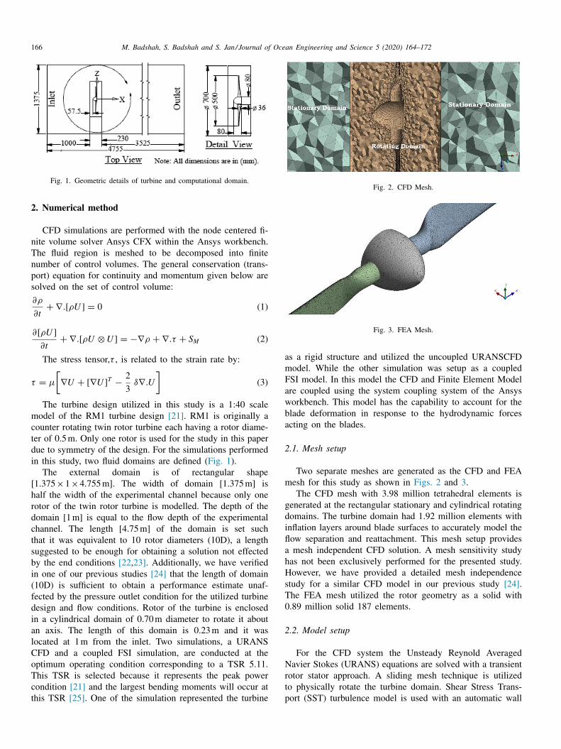
Fig. 1. Geometric details of turbine and computational domain.

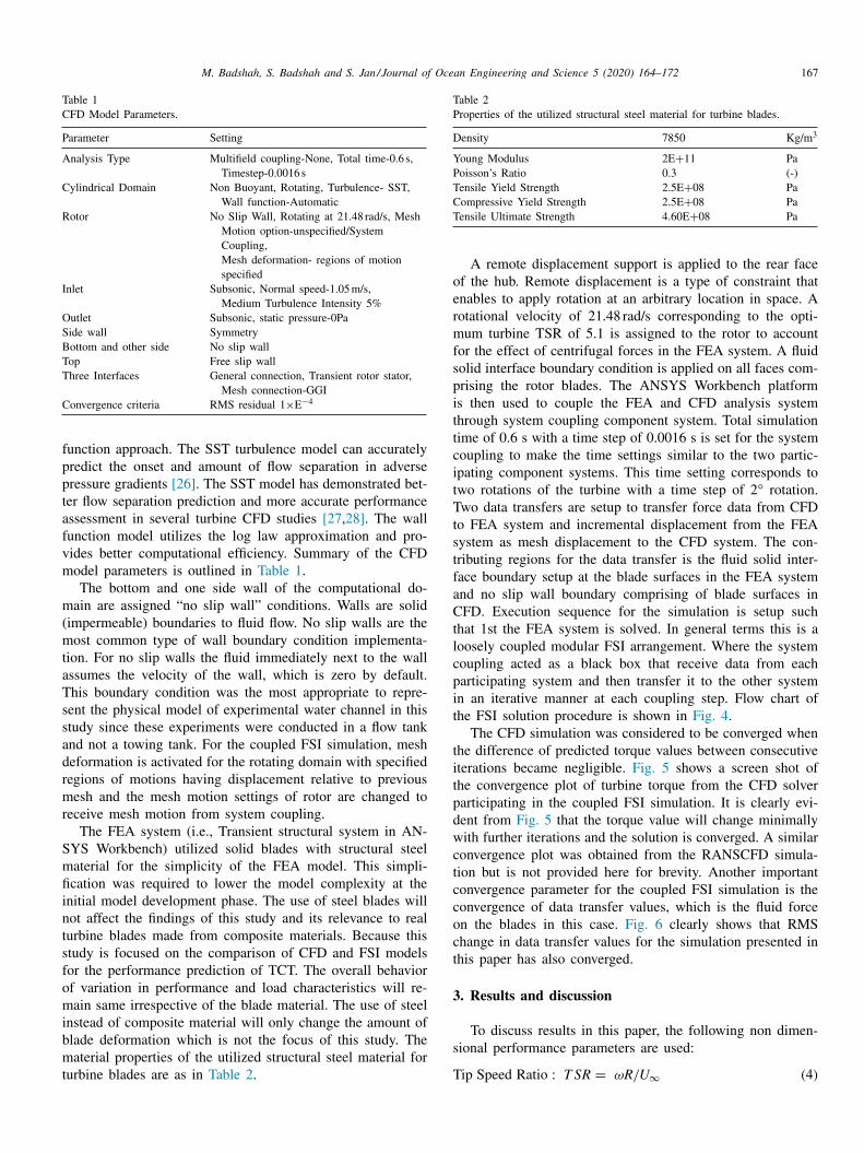
Fig. 2. CFD Mesh.

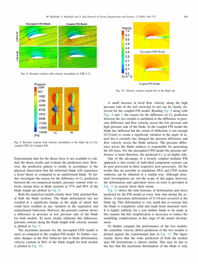
Fig. 3. FEA Mesh.

a

m

F

a

w

b

a

2

m

g

d

i

fl

a

h

H

s

T

0

2

N

r

t

p

2. Numerical method

CFD simulations are performed with the node centered fi-nite volume solver Ansys CFX within the Ansys workbench.The fluid region is meshed to be decomposed into finitenumber of control volumes. The general conservation (trans-port) equation for continuity and momentum given below aresolved on the set of control volume:

∂ρ

∂t + ∇. [ ρU ] = 0 (1)

∂ [ ρU ]

∂t + ∇. [ ρU � U ] = −∇ρ + ∇.τ + S M

(2)

The stress tensor, τ , is related to the strain rate by:

τ = μ

[∇ U + [ ∇ U ] T − 2

3

δ∇ .U

](3)

The turbine design utilized in this study is a 1:40 scalemodel of the RM1 turbine design [21] . RM1 is originally acounter rotating twin rotor turbine each having a rotor diame-ter of 0.5 m. Only one rotor is used for the study in this paperdue to symmetry of the design. For the simulations performedin this study, two fluid domains are defined ( Fig. 1 ).

The external domain is of rectangular shape[1.375 ×1 ×4.755 m]. The width of domain [1.375 m] ishalf the width of the experimental channel because only onerotor of the twin rotor turbine is modelled. The depth of thedomain [1 m] is equal to the flow depth of the experimentalchannel. The length [4.75 m] of the domain is set suchthat it was equivalent to 10 rotor diameters (10D), a lengthsuggested to be enough for obtaining a solution not effectedby the end conditions [22 , 23] . Additionally, we have verifiedin one of our previous studies [24] that the length of domain(10D) is sufficient to obtain a performance estimate unaf-fected by the pressure outlet condition for the utilized turbinedesign and flow conditions. Rotor of the turbine is enclosedin a cylindrical domain of 0.70 m diameter to rotate it aboutan axis. The length of this domain is 0.23 m and it waslocated at 1 m from the inlet. Two simulations, a URANSCFD and a coupled FSI simulation, are conducted at theoptimum operating condition corresponding to a TSR 5.11.This TSR is selected because it represents the peak powercondition [21] and the largest bending moments will occur atthis TSR [25] . One of the simulation represented the turbine

s a rigid structure and utilized the uncoupled URANSCFDodel. While the other simulation was setup as a coupledSI model. In this model the CFD and Finite Element Modelre coupled using the system coupling system of the Ansysorkbench. This model has the capability to account for thelade deformation in response to the hydrodynamic forcescting on the blades.

.1. Mesh setup

Two separate meshes are generated as the CFD and FEAesh for this study as shown in Figs. 2 and 3 . The CFD mesh with 3.98 million tetrahedral elements is

enerated at the rectangular stationary and cylindrical rotatingomains. The turbine domain had 1.92 million elements withnflation layers around blade surfaces to accurately model theow separation and reattachment. This mesh setup provides mesh independent CFD solution. A mesh sensitivity studyas not been exclusively performed for the presented study.owever, we have provided a detailed mesh independence

tudy for a similar CFD model in our previous study [24] .he FEA mesh utilized the rotor geometry as a solid with.89 million solid 187 elements.

.2. Model setup

For the CFD system the Unsteady Reynold Averagedavier Stokes (URANS) equations are solved with a transient

otor stator approach. A sliding mesh technique is utilizedo physically rotate the turbine domain. Shear Stress Trans-ort (SST) turbulence model is used with an automatic wall

M. Badshah, S. Badshah and S. Jan / Journal of Ocean Engineering and Science 5 (2020) 164–172 167

Table 1 CFD Model Parameters.

Parameter Setting

Analysis Type Multifield coupling-None, Total time-0.6 s, Timestep-0.0016 s

Cylindrical Domain Non Buoyant, Rotating, Turbulence- SST, Wall function-Automatic

Rotor No Slip Wall, Rotating at 21.48 rad/s, Mesh Motion option-unspecified/System

Coupling, Mesh deformation- regions of motion specified

Inlet Subsonic, Normal speed-1.05 m/s, Medium Turbulence Intensity 5%

Outlet Subsonic, static pressure-0Pa Side wall Symmetry Bottom and other side No slip wall Top Free slip wall Three Interfaces General connection, Transient rotor stator,

Mesh connection-GGI Convergence criteria RMS residual 1 ×E

−4

f

p

p

t

a

f

v

m

m

(

m

t

a

T

s

s

a

d

r

m

r

S

m

fi

i

n

t

s

f

o

m

i

b

m

t

Table 2 Properties of the utilized structural steel material for turbine blades.

Density 7850 Kg/m

3

Young Modulus 2E + 11 Pa Poisson’s Ratio 0.3 (-) Tensile Yield Strength 2.5E + 08 Pa Compressive Yield Strength 2.5E + 08 Pa Tensile Ultimate Strength 4.60E + 08 Pa

o

e

r

m

f

s

p

i

t

t

c

i

t

T

t

s

t

f

a

C

t

l

c

p

i

t

t

i

t

p

d

w

c

t

c

c

o

c

t

3

s

T

unction approach. The SST turbulence model can accuratelyredict the onset and amount of flow separation in adverseressure gradients [26] . The SST model has demonstrated bet-er flow separation prediction and more accurate performancessessment in several turbine CFD studies [27 , 28] . The wallunction model utilizes the log law approximation and pro-ides better computational efficiency. Summary of the CFDodel parameters is outlined in Table 1 . The bottom and one side wall of the computational do-

ain are assigned “no slip wall” conditions. Walls are solidimpermeable) boundaries to fluid flow. No slip walls are theost common type of wall boundary condition implementa-

ion. For no slip walls the fluid immediately next to the wallssumes the velocity of the wall, which is zero by default.his boundary condition was the most appropriate to repre-ent the physical model of experimental water channel in thistudy since these experiments were conducted in a flow tanknd not a towing tank. For the coupled FSI simulation, mesheformation is activated for the rotating domain with specifiedegions of motions having displacement relative to previousesh and the mesh motion settings of rotor are changed to

eceive mesh motion from system coupling. The FEA system (i.e., Transient structural system in AN-

YS Workbench) utilized solid blades with structural steelaterial for the simplicity of the FEA model. This simpli-cation was required to lower the model complexity at the

nitial model development phase. The use of steel blades willot affect the findings of this study and its relevance to realurbine blades made from composite materials. Because thistudy is focused on the comparison of CFD and FSI modelsor the performance prediction of TCT. The overall behaviorf variation in performance and load characteristics will re-ain same irrespective of the blade material. The use of steel

nstead of composite material will only change the amount oflade deformation which is not the focus of this study. Theaterial properties of the utilized structural steel material for

urbine blades are as in Table 2 .

A remote displacement support is applied to the rear facef the hub. Remote displacement is a type of constraint thatnables to apply rotation at an arbitrary location in space. Aotational velocity of 21.48 rad/s corresponding to the opti-um turbine TSR of 5.1 is assigned to the rotor to account

or the effect of centrifugal forces in the FEA system. A fluidolid interface boundary condition is applied on all faces com-rising the rotor blades. The ANSYS Workbench platforms then used to couple the FEA and CFD analysis systemhrough system coupling component system. Total simulationime of 0.6 s with a time step of 0.0016 s is set for the systemoupling to make the time settings similar to the two partic-pating component systems. This time setting corresponds towo rotations of the turbine with a time step of 2 ° rotation.wo data transfers are setup to transfer force data from CFD

o FEA system and incremental displacement from the FEAystem as mesh displacement to the CFD system. The con-ributing regions for the data transfer is the fluid solid inter-ace boundary setup at the blade surfaces in the FEA systemnd no slip wall boundary comprising of blade surfaces inFD. Execution sequence for the simulation is setup such

hat 1st the FEA system is solved. In general terms this is aoosely coupled modular FSI arrangement. Where the systemoupling acted as a black box that receive data from eacharticipating system and then transfer it to the other systemn an iterative manner at each coupling step. Flow chart ofhe FSI solution procedure is shown in Fig. 4 .

The CFD simulation was considered to be converged whenhe difference of predicted torque values between consecutiveterations became negligible. Fig. 5 shows a screen shot ofhe convergence plot of turbine torque from the CFD solverarticipating in the coupled FSI simulation. It is clearly evi-ent from Fig. 5 that the torque value will change minimallyith further iterations and the solution is converged. A similar

onvergence plot was obtained from the RANSCFD simula-ion but is not provided here for brevity. Another importantonvergence parameter for the coupled FSI simulation is theonvergence of data transfer values, which is the fluid forcen the blades in this case. Fig. 6 clearly shows that RMShange in data transfer values for the simulation presented inhis paper has also converged.

. Results and discussion

To discuss results in this paper, the following non dimen-ional performance parameters are used:

ip Speed Ratio : T SR = ωR/ U ∞

(4)

168 M. Badshah, S. Badshah and S. Jan / Journal of Ocean Engineering and Science 5 (2020) 164–172

Fig. 4. Loosely coupled modular FSI solution procedure.

Fig. 5. Convergence plot of turbine torque from the CFD solver participating in coupled FSI simulation.

Fig. 6. Convergence plot of data transfers from the coupled FSI simulation.

Fig. 7. Comparison of experimental and simulated performance coefficient.

Table 3 Quantitative comparison of Numerical and Experimental predictions.

Torque C P Thrust C P Error (N.m) (-) (N) (%)

Experiment 2.08 0.4337 – –Uncoupled CFD Model 2.28 0.4761 100.22 9.78 Coupled FSI Model 2.18 0.4545 99.29 4.80

n

t

C

d

d

l

v

p

i

p

m

f

m

d

Power Coefficient : C P = P/ 0. 5 ρAU

3 ∞

(5)

Thrust Coefficient : C T = T / 0. 5 ρAU

2 ∞

(6)

In these equations U ∞

(m/s) represent the free stream ve-locity, ω (rad/s) the angular speed of the blade tip (assumedconstant for the simulations conducted in this paper), R (m)the radius of the rotor, A (m

2 ) the swept area of the rotor, P(watts) the total power available in the flow stream and T (N)is the force acting along the flow direction.

To compare the accuracy of the utilized modelling tech-iques the simulated results are plotted against the experimen-al data [21] . Fig. 7 shows the comparison of power coefficient P obtained from the CFD simulations and experiments.

The quantitative comparison of experimental data and pre-ictions of the numerical models are as in Table 3 .

The difference between experimental value of C P and pre-icted value from the rigid blade CFD and FSI models wasess than 10%. The coupled FSI model predicted a loweralue of turbine C P (0.45) compared to a C P value of 0.48redicted by the uncoupled rigid blade CFD model. Thiss in contrast to Tatum et al. [19] where the FSI modelredicted a greater value of C P than the uncoupled CFDodel. Tatum et al. [19] attributed this discrepancy to the

act that initially blades of their turbine were not in its opti-um position. A thrust force of 100.22 N and 99.29 N is pre-

icted by the uncoupled CFD and FSI models respectively.

M. Badshah, S. Badshah and S. Jan / Journal of Ocean Engineering and Science 5 (2020) 164–172 169

Fig. 8. Pressure contour with velocity streamlines at TSR 5.11.

Fig. 9. Pressure contour with velocity streamlines at the blade tip (a) Un- coupled CFD (b) Coupled FSI.

E

d

e

p

a

t

b

l

b

a

r

c

r

a

f

p

i

m

a

v

i

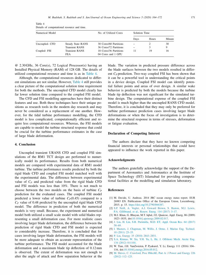
Fig. 10. Velocity contour around foil at the blade tip.

p

s

F

b

s

h

b

(

t

fl

e

t

f

a

b

r

s

t

t

F

p

l

b

t

I

t

m

m

t

p

c

u

t

xperimental data for the thrust force is not available to vali-ate the thrust results and evaluate the prediction error. How-ver, the prediction pattern is totally in accordance to thehysical observation that the deformed blade will experience lesser thrust as compared to an undeformed blade. To fur-her investigate the reason for the difference in C P predictionetween the two numerical models, pressure contour with ve-ocity stream lines at blade sections at 37% and 96% of thelade length are plotted in Fig. 8 .

Both the numerical models clearly show fully attached flowt both the blade sections. The blade deformation has notesulted in a significant change in the angle of attack thatould have resulted in any variation in the separation andeattachment behaviour. However, the pressure contour shows difference in pressure at low pressure side of the bladeor both models. To more clearly elaborate this difference,ressure contour along the blade length with velocity streamss plotted in Fig. 9 .

The maximum pressure for the uncoupled CFD model isore as compared to the coupled FSI model. To further visu-

lize changes in the flow behavior due to blade deformation,elocity contour at 96% of the blade length for both modelss plotted in Fig. 10 .

A small increase in local flow velocity along the highressure side of the foil encircled in red can be clearly ob-erved for the coupled FSI model. Reading Fig. 5 along withigs. 6 and 7 , the reason for the difference in C P predictionetween the two models is attributed to the difference in pres-ure difference and flow velocity across the low pressure andigh pressure side of the blade. In the coupled FSI model thelade has deflected but the extent of deflection is not enough0.12 mm) to create a significant variation in the angle of at-ack but it certainly has changed the pressure difference andow velocity across the blade surfaces. The pressure differ-nce across the blade surfaces is responsible for generatinghe lift force. For the uncoupled CFD model the pressure dif-erence is more therefore, the predicted C P is on higher side.

One of the advantage of a loosely coupled modular FSIpproach is that results of individual component systems cane post processed in their respective post processors. All theesults that are possible in standalone FEA and CFD systemolutions can be obtained in a similar way. Although struc-ural investigations are not the scope of this paper, however,he deformation and equivalent stress on rotor is provided inig. 11 to exactly know their extent.

Fig. 12 shows the time histories of deformation and stressredicted by the FSI model at every time step during the so-ution. A maximum deformation of 0.116 mm occurred at thelade tip. This deformation is very small due to reasons thathe blade is completely solid and made from structural steel.t is highly unlikely for a real turbine blade to be made inhis manner but this simplification is necessary to reduce theodelling complications at this stage of the model develop-ent. To further compare the performance of the two models,

he centerline velocity deficit prediction of the two models islotted against the experimental data in Fig. 13 . The figurelearly shows that the wake prediction of both the modelspto 6D downstream is almost similar. This may be due tohe fact that the maximum deformation of the blade is only

170 M. Badshah, S. Badshah and S. Jan / Journal of Ocean Engineering and Science 5 (2020) 164–172

Fig. 11. Stress and deformation contour at the rotor.

Fig. 12. Stress and deformation at the rotor at every time step during the FSI solution process.

Fig. 13. Comparison of rotor hub height velocity deficit prediction.

Fig. 14. Velocity vectors plotted on a vertical plan along the rotor center line (a) Uncoupled CFD model (b) Coupled FSI Model.

u

o

t

a

t

d

s

m

t

m

s

s

d

w

o

u

i

f

i

a

p

r

v

u

Z

0.12 mm which is not expected to make a huge difference inthe wake prediction. The other important aspect of the wakeresults is that the prediction of both models does not conformto the experimental data. This could be due to the effect ofcross arms, tower and left side rotor. These effects are notincluded in the numerical model for simplicity. Additionally,the simulations presented in this paper utilized CFD based onReynolds Averaged Navier Stokes (RANS) models. In this ap-proach the time averaged Navier–Stokes equation are solvedthrough turbulence model to solve all the turbulent lengthscales. An SST turbulence model belonging to the group ofeddy viscosity model based on the Boussinesq hypothesis is

sed. The Boussinesq hypothesis is based on the assumptionf isotropic turbulence, which is only valid for small scaleurbulence. On the contrary, turbulence in the wake region of TCT is strongly anisotropic in nature [29] and the size ofurbulence structure is of the same order of magnitude as theiameter of turbine [30] . The accurate modelling of down-tream wake would require Large Eddy Simulations (LES)odels that solves the spatially averaged Navier-Stokes equa-

ions and directly resolve large turbulence structures. Further-ore, the experimental wake data is upto 25D whereas the

imulated wake data is upto 7D. To obtain a clear compari-on between the experimental and numerical velocity deficitata, a farther velocity deficit plot from the numerical modelill be required. Since far wake study is not the objectivef this work, therefore, a shorter domain length of 10D issed to achieve a better computational efficiency. To gain annsight of the flow passing through the turbine, the stationaryrame velocity vectors are plotted along a vertical plane pass-ng through the centerline of the rotor (see Fig. 14 ). Almost similar flow behavior has been captured by both models.

Although both the numerical models predict the turbineerformance and wake with almost similar accuracy but theequirement of computational resource and solution time areery different. Both the uncoupled CFD and coupled FSI sim-lations presented in this paper are performed on the HP840 Workstation with Intel(R) Xeon(R) CPU E5-2699 v3

M. Badshah, S. Badshah and S. Jan / Journal of Ocean Engineering and Science 5 (2020) 164–172 171

Table 4 Details of computational resource and time.

Numerical Model No. of Utilized Cores Solution Time

Days Hours Minute

Uncoupled- CFD Steady State RANS 30 Cores/60 Partitions – 2 30 Transient RANS 36 Cores/72 Partitions – 3 9

Coupled- FSI Transient RANS 18 Cores/36 Partitions 11 19 16 FEA 04 Cores and 1 GPU

@

I

u

e

a

f

f

f

s

n

e

m

q

a

b

o

4

u

i

m

t

r

t

v

a

cp

p

C

m

m

m

r

i

p

t

c

b

t

d

i

a

b

t

e

i

i

t

b

b

b

m

T

t

d

m

o

D

fi

a

A

p

S

t

R

2.30 GHz, 36 Core(s), 72 Logical Processor(s) having annstalled Physical Memory (RAM) of 128 GB. The details oftilized computational resource and time is as in Table 4 .

Although, the computational resources dedicated to differ-nt simulations are not similar. However, Table 4 still provides clear picture of the computational solution time requirementor both the methods. The uncoupled CFD model clearly hasar lower solution time compared to the coupled FSI model.

The CFD and FSI modelling approaches have their distincteatures and use. Both these techniques have their unique po-itions as research tools in the modern day research and mayever be considered as a replacement of one another. How-ver, for the tidal turbine performance modelling, the CFDodel is less complicated, computationally efficient and re-

uire less computational resources. Whereas, the FSI modelsre capable to model the turbine structural response that coulde crucial for the turbine performance estimates in the casef large blade deformation.

. Conclusion

Uncoupled transient URANS CFD and coupled FSI sim-lations of the RM1 TCT design are performed to numer-cally model its performance. Results from both numericalodels are compared with experimental data of RM1 model

urbine. The turbine performance results predicted by both theigid blade CFD and coupled FSI model matched well withhe experimental data. The difference between experimentalalue of C P and predicted value from the rigid blade CFDnd FSI models was less than 10%. There is not much tohoose between the two models on the basis of turbine C P

rediction for the evaluated cases. The coupled FSI modelredicted a lower value of turbine C P (0.45) compared to a P value of 0.48 predicted by the uncoupled rigid blade CFDodel. The difference in prediction of both the numericalodels is very small. Because, the experiment and numericalodel both utilized a small scale model with solid blades rep-

esenting a small deformation case. For more realistic casesnvolving larger blade deformation, the difference between therediction of rigid blade CFD and FSI model is expectedo considerably increase. Therefore, it is concluded that forases involving larger blade deformation, the FSI models wille more adequate to obtain an accurate representation of theurbine performance. The FSI model accounted for the bladeeformation and a maximum blade tip deflection of 0.12 mms observed. The extent of deformation was not enough tolter the angle of attack and flow separation behavior at the

lade. The variation in predicted pressure difference acrosshe blade surfaces between the two models resulted in differ-nt C P prediction. Two-way coupled FSI has been shown thatt can be a powerful tool in understanding the critical pointsn a device design. Coupled FSI model can identify poten-ial failure points and areas of over design. A similar wakeehavior is predicted by both the models because the turbinelade tip deflection was not significant for the simulated tur-ine design. The computational expense of the coupled FSIodel is much higher than the uncoupled RANS CFD model.herefore, it is concluded that they may only be preferred for

urbine performance prediction cases involving larger bladeeformations or when the focus of investigation is to deter-ine the structural response in terms of stresses, deformation

r fatigue evaluation.

eclaration of Competing Interest

The authors declare that they have no known competingnancial interests or personal relationships that could haveppeared to influence the work reported in this paper.

cknowledgments

The authors gratefully acknowledge the support of the De-artment of Aeronautics and Astronautics at the Institute ofpace Technology (IST) Islamabad for providing computa-

ional facilities at the modelling and simulation laboratory.

eferences

[1] M. Davide, U. Andreas. 2014 JRC ocean energy status report. EUR26983 EN. Publications Office of the European Union, Luxembourg,2015. p. 15. https:// doi.org/ 10.2790/ 866387 .

[2] S.P. Neill , A. Vogler , A.J. Goward Brown , S. Baston , M.J. Lewis ,P.A. Gillibrand , et al. , Renew. Energ. 114 (2017) 3–17 .

[3] M.J. Khan, G. Bhuyan, M.T. Iqbal, J.E. Quaicoe, Appl. Energ. 86 (2009)1823–1835, doi: 10.1016/j.apenergy.2009.02.017 .

[4] J. Liu , H. Lin , S.R. Purimitla , M.D. ET , Appl. Ocean Res. 64 (2017)58–69 .

[5] I. Masters , J. Chapman , M. Willis , J. Orme , J. Marine Eng. Technol.10 (2011) 25–35 .

[6] P. Liu , Energy 35 (2010) 2843–2851 . [7] S.A. Kinnas , W. Xu , Y.H. Yu , L. He , J. Offshore Mech. Arctic Eng.

134 (2012) 011101 . [8] W. Tian, J.H. VanZwieten, P. Pyakurel, Y. Li, Energy 111 (2016) 104–

116, doi: 10.1016/j.energy.2016.05.012. [9] M. Shives , C. Crawford , Proc IMechE, Part A: J Power and Energy 226

(2012) 112–125 .

172 M. Badshah, S. Badshah and S. Jan / Journal of Ocean Engineering and Science 5 (2020) 164–172

[

[

[

[

[

[

[

[[[

[10] R.F. Nicholls-Lee , S.R. Turnock , S.W. Boyd , in: Proceedings of the7th International Conference on Computer and IT Applications in theMaritime Industries (COMPIT’08), 2008, pp. 314–328 .

[11] G. Hou , J. Wang , A. Layton , Commun. Comput. Phys. 12 (2012)337–377 .

[12] M. Badshah , S. Badshah , K. Kadir , Energies 11 (2018) 1–13 . [13] S. Turnock, A. Wright, Mar. Struct. 13 (2000) 53–72, doi: 10.1016/

S0951- 8339(00)00009- 5 . [14] B. Kim, S. Bae, W. Kim, S. Lee, M. Kim, in: IOP Conf. Series:

Earth and Environmental Science, 2012, doi: 10.1088/ 1755-1315/ 15/ 4/042037042037 .

[15] C.-.H. Jo , D.-.Y. Kim , Y.-.H. Rho , K.-.H. Lee , C. Johnstone , Renew.Energy 54 (2013) 248–252 .

[16] U. Habib , M. Hussain , N. Abbas , H. Ahmad , M. Amer , M. Noman , J.Ocean Eng. Sci. (2019) .

[17] R. Nicholls-Lee , S. Turnock , S. Boyd , Renew. Energy 50 (2013)541–550 .

[18] T. Suzuki , H. Mahfuz , Ships Off Shore Struct. 13 (2018) 451–458 . [19] S.C. Tatum, C.H. Frost, M. Allmark, D.M. O’Doherty, A. Mason-Jones,

P.W. Prickett, et al., Int. J. Mar. Energy 14 (2016) 161–179, doi: 10.1016/j.ijome.2015.09.002.

[20] M. Badshah , S. Badshah , J. VanZwieten , S. Jan , M. Amir , S.A. Malik ,Energies 12 (2019) 2217 .

21] H. Craig, S.N. Vincent, G. Budi, G. Michele, S. Fotis, U.S. De-partment of Energy Reference Model Program RM1: ExperimentalResults. Technical Report; 2014. Available online: https://www.osti.gov/ biblio/ 1172793- department- energy- reference- model- program- rm1- experimental-results , doi: 10.2172/1172793 , (accessed on 19 th October2019).

22] H.J. Chul, Y.Y. Jin, H.L. Kang, H.R. Yu, Renew. Energ. 42 (2011)195–206, doi: 10.1016/j.renene.2011.08.017 .

23] K. Nitin, B. Arindam, Appl. Energ. 148 (2015) 121–133, doi: 10.1016/j.apenergy.2015.03.052.

24] M. Badshah, J. VanZwieten, S. Badshah, S. Jan, IET Renew. PowerGen. (2019), doi: 10.1049/iet-rpg.2018.5134.

25] P. Ouro , M. Harrold , T. Stoesser , P. Bromley , J. Fluids Struct. 71 (2017)78–95 .

26] ANSYS Inc., ANSYS CFX-Solver Modelling Guide, ANSYS Inc.,Canonsburg, PA, USA, 2016, p. 146 .

27] S.F. Sufian, M. Li, B.A. O’Connor, Renew. Energ. 114 (2017) 308–322,doi: 10.1016/j.renene.2017.04.030.

28] A. Elhanafi, J. Ocean Eng. Sci. 1 (2016) 268–283 . 29] S. Tedds , I. Owen , R. Poole , Renew. Energ. 63 (2014) 222–235 . 30] I.A. Milne , R.N. Sharma , R.G. Flay , S. Bickerton , Philos. Trans. R.

Soc. A 371 (2013) 20120196 .