Embed Size (px)
Citation preview

6.02 Fall 2012 Lecture #11
• Eye diagrams • Alternative ways to look at convolution
6.02 Fall 2012 Lecture 11, Slide #1

Eye Diagrams
000 100 010 110 001 101 011 111
These are overlaidEye diagrams make it easy to find two-bit-slot segmentsthe worst-case signaling conditions of step responses, plottedat the receiving end. without the ‘stems’ of the stem plot on the left6.02 Fall 2012 Lecture 11, Slide #2

“Width” of Eye Worst-case “1”
Worst-case “0” “width” of eye (as in “eye wide open”)
To maximize noise margins: Pick the best sample point � widest point in the eye
Pick the best digitization threshold � half-way across width
6.02 Fall 2012 Lecture 11, Slide #3

Choosing Samples/Bit
Oops, no eye!ye!
Given h[n], you can use the eye diagram to pick the number of samples transmitted for each bit (N):
Reduce N until you reach the noise margin you feel is the minimum acceptable value.
6.02 Fall 2012 Lecture 11, Slide #4

Example: “ringing” channel
6.02 Fall 2012 Lecture 11, Slide #5

Constructing the Eye Diagram (no need to wade through all this unless you
really want to!)
1. Generate an input bit sequence pattern that contains all possible combinations of B bits (e.g., B=3 or 4), so a sequence of 2BB bits. (Otherwise, a random sequence of comparable length is fine.)
2. Transmit the corresponding x[n] over the channel (2BBN samples, if there are N samples/bit)
3. Instead of one long plot of y[n], plot the response as an eye diagram: a. break the plot up into short segments, each containing
KN samples, starting at sample 0, KN, 2KN, 3KN, … (e.g., K=2 or 3)
b. plot all the short segments on top of each other
6.02 Fall 2012 Lecture 11, Slide #6

Back To Convolution From last lecture: If system S is both linear and time-invariant (LTI), then we can use the unit sample response h[n] to predict the response to any input waveform x[n]:
Sum of shifted, scaled unit sample Sum of shifted, scaled unit sample functions responses, with the same scale factors
∞
S ∞
x[n] = ∑ x[k]δ[n − k] y[n] = ∑ x[k]h[n − k] k=−∞ k=−∞
CONVOLUTION SUM
Indeed, the unit sample response h[n] completely characterizes the LTI system S, so you often see
h[.]x[n] y[n]
6.02 Fall 2012 Lecture 11, Slide #7

�
Sx[n]
Unit Sample Response of a Scale-&-Delay System
y[n]=Ax[n-D]
If S is a system that scales the input by A and delays it by D time steps (negative ‘delay’ D = advance), is the system
time-invariant? Yes!
linear? Yes!
Unit sample response is h[n]=Aδ[n-D]
General unit sample response
h[n]=… + h[-1] δ[n+1] + h[0]δ[n] + h[1]δ[n�1]+… �
for an LTI system can be thought of as resulting from 6.02 Fall 2012 many scale-&-delays in parallel Lecture 11, Slide #8

A Complementary View of Convolution So instead of the picture:
∞ ∞
x[n] = ∑ x[k]δ[n − k] y[n] = ∑ x[k]h[n − k] k=−∞ k=−∞
we can consider the picture:
h[.]
h[.]=…+h[-1]δ[n+1]+h[0]δ[n]+h[1]δ[n-1]+…x[n] y[n]
∞
from which we get y[n] = ∑ h[m]x[n − m] m=−∞
(To those who have an eye for these things, my apologies 6.02 Fall 2012 for the varied math font --- too hard to keep uniform!) Lecture 11, Slide #9

(side by side) y[n] =
∞ ∞
(x ∗ h)[n] = ∑ x[k]h[n − k] = ∑ h[m]x[n − m] = (h ∗ x)[n ] k=−∞ m=−∞
Input term x[0] at Unit sample response time 0 launches term h[0] at time 0 scaled unit sample contributes scaled input response x[0]h[n] at h[0]x[n] to output output
Input term x[k] at Unit sample response time k launches term h[m] at time m scaled shifted unit contributes scaled shifted sample response input h[m]x[n-m] x[k]h[n-k] at output to output
6.02 Fall 2012 Lecture 11, Slide #10

To Convolve (but not to “Convolute”!) ∞ ∞
∑ x[k]h[n − k] = ∑ h[m]x[n − m] k=−∞ m=−∞
A simple graphical implementation:
Plot x[.] and h[.] as a function of the dummy index (k or m above)
Flip (i.e., reverse) one signal in time, slide it right by n (slide left if n is –ve), take the dot.product with the other.
This yields the value of the convolution at the single time n.
‘flip one & slide by n …. dot.product with the other’
6.02 Fall 2012 Lecture 11, Slide #11

Example • From the unit sample response h[n] to the unit step response
s[n] = (h *u)[n]
• Flip u[k] to get u[-k] • Slide u[-k] n steps to right (i.e., delay u[-k]) to get u[n-k]),
place over h[k] • Dot product of h[k] and u[n-k] wrt k:
n
s[n] = ∑ h[k] k=−∞
6.02 Fall 2012 Lecture 11, Slide #12

Channels as LTI Systems
Many transmission channels can be effectively modeled as LTI systems. When modeling transmissions, there are few simplifications we can make:
• We’ll call the time transmissions start t=0; the signal before the start is 0. So x[m] = 0 for m < 0.
• Real-word channels are causal: the output at any time depends on values of the input at only the present and past times. So h[m] = 0 for m < 0.
These two observations allow us to rework the convolution sum when it’s used to describe transmission channels:
∞ ∞ n n
y[n] = ∑ x[k]h[n − k] = ∑x[k]h[n − k ∑] = x[k]h[n − k] = ∑x[n − j]h[ j] k=−∞ k=0 k=0 j=0
6.02 Fall 2012 start at t=0 causal j=n-k Lecture 11, Slide #13
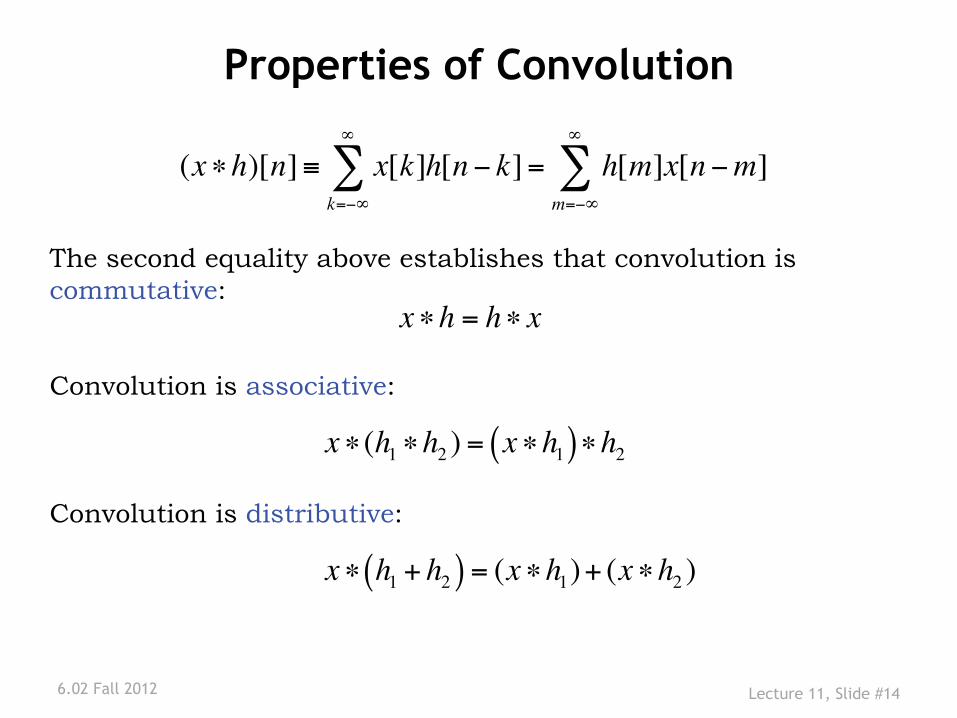
Properties of Convolution ∞ ∞
(x ∗ h)[n] ≡ ∑ x[k]h[n − k] = ∑ h[m]x[n − m] k=−∞ m=−∞
The second equality above establishes that convolution is commutative:
x ∗ h = h ∗ x
Convolution is associative:
x ∗ (h1 ∗ h2 ) = (x ∗ h1 )∗ h2
Convolution is distributive:
x ∗(h1 + h2 ) = (x ∗ h1) + (x ∗ h2 )
6.02 Fall 2012 Lecture 11, Slide #14

Series Interconnection of LTI Systems
x[n] h1[.] h2[.] w[n]
y[n]
y = h2 ∗ w = h2 ∗(h1 ∗ x) = (h2 ∗ h1 )∗ x
(h2 *h1)[.]x[n] y[n]
(h1 *h2)[.]x[n] y[n]
h2[.]x[n] h1[.] y[n]
6.02 Fall 2012 Lecture 11, Slide #15

“Deconvolving” Output of Echo Channel
Channel, h1[.]
Receiver filter, h2[.]
x[n] y[n] z[n]
Suppose channel is LTI with
h 1[n]=δ[n]+0.8δ[n-1]
Find h2[n] such that z[n]=x[n]
(h2*h1)[n]=δ[n]
Good exercise in applying Flip/Slide/Dot.Product
6.02 Fall 2012 Lecture 11, Slide #16

“Deconvolving” Output of Channel with Echo
Channel, h1[.]
Receiver filter, h2[.]
x[n] y[n] +
z[n]+v[n]
w[n]
Even if channel was well modeled as LTI and h1[n] was known, noise on the channel can greatly degrade the result, so this is usually not practical.
6.02 Fall 2012 Lecture 11, Slide #17
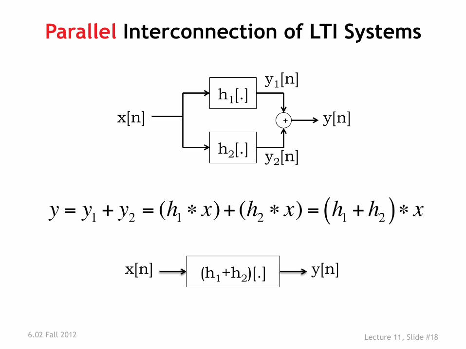
Parallel Interconnection of LTI Systems
h1[.]
x[n]
y1[n]
h2[.]
+
y2[n]
y[n]
y = y1 + y2 = (h1 ∗ x) + (h2 ∗ x) = (h1 + h2 )∗ x
(h1+h2)[.]x[n] y[n]
6.02 Fall 2012 Lecture 11, Slide #18

MIT OpenCourseWarehttp://ocw.mit.edu
6.02 Introduction to EECS II: Digital Communication SystemsFall 2012
For information about citing these materials or our Terms of Use, visit: http://ocw.mit.edu/terms.


![A Class of LTI Distributed Observers for LTI Plants ...1401.0926v1 [cs.SY] 5 Jan 2014 1 A Class of LTI Distributed Observers for LTI Plants: Necessary and Sufficient Conditions for](https://img.dokumen.tips/doc/110x75/5afedcd17f8b9a256b8da98c/a-class-of-lti-distributed-observers-for-lti-plants-14010926v1-cssy-5-jan.jpg)