Embed Size (px)
Citation preview

Contents
3 Equalization 1493.1 Intersymbol Interference and Receivers for Successive Message Transmission . . . . . . . . 151
3.1.1 Transmission of Successive Messages . . . . . . . . . . . . . . . . . . . . . . . . . . 1513.1.2 Bandlimited Channels . . . . . . . . . . . . . . . . . . . . . . . . . . . . . . . . . . 1523.1.3 The ISI-Channel Model . . . . . . . . . . . . . . . . . . . . . . . . . . . . . . . . . 157
3.2 Basics of the Receiver-generated Equivalent AWGN . . . . . . . . . . . . . . . . . . . . . 1643.2.1 Receiver Signal-to-Noise Ratio . . . . . . . . . . . . . . . . . . . . . . . . . . . . . 1643.2.2 Receiver Biases . . . . . . . . . . . . . . . . . . . . . . . . . . . . . . . . . . . . . . 1653.2.3 The Matched-Filter Bound . . . . . . . . . . . . . . . . . . . . . . . . . . . . . . . 167
3.3 Nyquist’s Criterion . . . . . . . . . . . . . . . . . . . . . . . . . . . . . . . . . . . . . . . . 1703.3.1 Vestigial Symmetry . . . . . . . . . . . . . . . . . . . . . . . . . . . . . . . . . . . 1713.3.2 Raised Cosine Pulses . . . . . . . . . . . . . . . . . . . . . . . . . . . . . . . . . . . 1723.3.3 Square-Root Splitting of the Nyquist Pulse . . . . . . . . . . . . . . . . . . . . . . 174
3.4 Linear Zero-Forcing Equalization . . . . . . . . . . . . . . . . . . . . . . . . . . . . . . . . 1763.4.1 Performance Analysis of the ZFE . . . . . . . . . . . . . . . . . . . . . . . . . . . . 1763.4.2 Noise Enhancement . . . . . . . . . . . . . . . . . . . . . . . . . . . . . . . . . . . 178
3.5 Minimum Mean-Square Error Linear Equalization . . . . . . . . . . . . . . . . . . . . . . 1863.5.1 Optimization of the Linear Equalizer . . . . . . . . . . . . . . . . . . . . . . . . . . 1863.5.2 Performance of the MMSE-LE . . . . . . . . . . . . . . . . . . . . . . . . . . . . . 1873.5.3 Examples Revisited . . . . . . . . . . . . . . . . . . . . . . . . . . . . . . . . . . . 1893.5.4 Fractionally Spaced Equalization . . . . . . . . . . . . . . . . . . . . . . . . . . . . 193
3.6 Decision Feedback Equalization . . . . . . . . . . . . . . . . . . . . . . . . . . . . . . . . 1983.6.1 Minimum-Mean-Square-Error Decision Feedback Equalizer (MMSE-DFE) . . . . . 1983.6.2 Performance Analysis of the MMSE-DFE . . . . . . . . . . . . . . . . . . . . . . . 2003.6.3 Zero-Forcing DFE . . . . . . . . . . . . . . . . . . . . . . . . . . . . . . . . . . . . 2023.6.4 Examples Revisited . . . . . . . . . . . . . . . . . . . . . . . . . . . . . . . . . . . 203
3.7 Finite Length Equalizers . . . . . . . . . . . . . . . . . . . . . . . . . . . . . . . . . . . . 2073.7.1 FIR MMSE-LE . . . . . . . . . . . . . . . . . . . . . . . . . . . . . . . . . . . . . . 2073.7.2 FIR ZFE . . . . . . . . . . . . . . . . . . . . . . . . . . . . . . . . . . . . . . . . . 2103.7.3 example . . . . . . . . . . . . . . . . . . . . . . . . . . . . . . . . . . . . . . . . . . 2113.7.4 FIR MMSE-DFE . . . . . . . . . . . . . . . . . . . . . . . . . . . . . . . . . . . . . 2133.7.5 An Alternative Approach to the DFE . . . . . . . . . . . . . . . . . . . . . . . . . 2183.7.6 The Stanford DFE Program . . . . . . . . . . . . . . . . . . . . . . . . . . . . . . . 2223.7.7 Error Propagation in the DFE . . . . . . . . . . . . . . . . . . . . . . . . . . . . . 2243.7.8 Look-Ahead . . . . . . . . . . . . . . . . . . . . . . . . . . . . . . . . . . . . . . . . 227
3.8 Precoding . . . . . . . . . . . . . . . . . . . . . . . . . . . . . . . . . . . . . . . . . . . . . 2283.8.1 The Tomlinson Precoder . . . . . . . . . . . . . . . . . . . . . . . . . . . . . . . . . 2283.8.2 Partial Response Channel Models . . . . . . . . . . . . . . . . . . . . . . . . . . . 2343.8.3 Classes of Partial Response . . . . . . . . . . . . . . . . . . . . . . . . . . . . . . . 2363.8.4 Simple Precoding . . . . . . . . . . . . . . . . . . . . . . . . . . . . . . . . . . . . . 2393.8.5 General Precoding . . . . . . . . . . . . . . . . . . . . . . . . . . . . . . . . . . . . 2433.8.6 Quadrature PR . . . . . . . . . . . . . . . . . . . . . . . . . . . . . . . . . . . . . . 244
147
3.9 Diversity Equalization . . . . . . . . . . . . . . . . . . . . . . . . . . . . . . . . . . . . . . 2473.9.1 Multiple Received Signals and the RAKE . . . . . . . . . . . . . . . . . . . . . . . 2473.9.2 Infinite-length MMSE Equalization Structures . . . . . . . . . . . . . . . . . . . . 2493.9.3 Finite-length Multidimensional Equalizers . . . . . . . . . . . . . . . . . . . . . . . 2513.9.4 DFE RAKE Program . . . . . . . . . . . . . . . . . . . . . . . . . . . . . . . . . . 2523.9.5 Multichannel Transmission . . . . . . . . . . . . . . . . . . . . . . . . . . . . . . . 254
Exercises - Chapter 3 . . . . . . . . . . . . . . . . . . . . . . . . . . . . . . . . . . . . . . . . . 256
A Useful Results in Linear Minimum Mean-Square Estimation 279A.1 The Orthogonality Principle . . . . . . . . . . . . . . . . . . . . . . . . . . . . . . . . . . . 279A.2 Spectral Factorization . . . . . . . . . . . . . . . . . . . . . . . . . . . . . . . . . . . . . . 280
A.2.1 Cholesky Factorization . . . . . . . . . . . . . . . . . . . . . . . . . . . . . . . . . . 281
B Equalization for Partial Response 286B.1 Controlled ISI with the DFE . . . . . . . . . . . . . . . . . . . . . . . . . . . . . . . . . . 286
B.1.1 ZF-DFE and the Optimum Sequence Detector . . . . . . . . . . . . . . . . . . . . 286B.1.2 MMSE-DFE and sequence detection . . . . . . . . . . . . . . . . . . . . . . . . . . 288
B.2 Equalization with Fixed Partial Response B(D) . . . . . . . . . . . . . . . . . . . . . . . . 288B.2.1 The Partial Response Linear Equalization Case . . . . . . . . . . . . . . . . . . . . 288B.2.2 The Partial-Response Decision Feedback Equalizer . . . . . . . . . . . . . . . . . . 289
C The Matrix Inversion Lemma: 291
148

Chapter 3
Equalization
The main focus of Chapter 1 was a single use of the channel, signal set, and detector to transmit oneof M messages, commonly referred to as “one-shot” transmission. In practice, the transmission systemsends a sequence of messages, one after another, in which case the analysis of Chapter 1 applies onlyif the channel is memoryless: that is, for one-shot analysis to apply, these successive transmissionsmust not interfere with one another. In practice, successive transmissions do often interfere with oneanother, especially as they are spaced more closely together to increase the data transmission rate.The interference between successive transmissions is called intersymbol interference (ISI). ISI canseverely complicate the implementation of an optimum detector.
Figure 3.1 illustrates a receiver for detection of a succession of messages. The matched filter outputsare processed by the receiver, which outputs samples, zk, that estimate the symbol transmitted at timek, xk. Each receiver output sample is the input to the same one-shot detector that would be used on anAWGN channel without ISI. This symbol-by-symbol (SBS) detector, while optimum for the AWGNchannel, will not be a maximum-likelihood estimator for the sequence of messages. Nonetheless, if thereceiver is well-designed, the combination of receiver and detector may work nearly as well as an optimumdetector with far less complexity. The objective of the receiver will be to improve the performance ofthis simple SBS detector. More sophisticated and complex sequence detectors are the topics of Chapters4, 5 and 9.
Equalization methods are used by communication engineers to mitigate the effects of the intersym-bol interference. An equalizer is essentially the content of Figure 3.1’s receiver box. This chapter studiesboth intersymbol interference and several equalization methods, which amount to different structuresfor the receiver box. The methods presented in this chapter are not optimal for detection, but rather arewidely used sub-optimal cost-effective methods that reduce the ISI. These equalization methods try toconvert a bandlimited channel with ISI into one that appears memoryless, hopefully synthesizing a newAWGN-like channel at the receiver output. The designer can then analyze the resulting memoryless,equalized channel using the methods of Chapter 1. With an appropriate choice of transmit signals,one of the methods in this chapter - the Decision Feedback Equalizer of Section 3.6 can be generalizedinto a canonical receiver (effectively achieves the highest possible transmission rate even though not anoptimum receiver), which is discussed further in Chapter 5 and occurs only when special conditions aremet.
Section 3.1 models linear intersymbol interference between successive transmissions, thereby bothillustrating and measuring the problem. In practice, as shown by a simple example, distortion fromoverlapping symbols can be unacceptable, suggesting that some corrective action must be taken. Section3.1 also refines the concept of signal-to-noise ratio, which is the method used in this text to quantifyreceiver performance. The SNR concept will be used consistently throughout the remainder of this textas a quick and accurate means of quantifying transmission performance, as opposed to probability oferror, which can be more difficult to compute, especially for suboptimum designs. As Figure 3.1 shows,the objective of the receiver will be to convert the channel into an equivalent AWGN at each time k,independent of all other times k. An AWGN detector may then be applied to the derived channel, andperformance computed readily using the gap approximation or other known formulae of Chapters 1 and
149

Figure 3.1: The band-limited channel with receiver and SBS detector.
2 with the SNR of the derived AWGN channel. There may be loss of optimality in creating such anequivalent AWGN, which will be measured by the SNR of the equivalent AWGN with respect to the bestvalue that might be expected otherwise for an optimum detector. Section 3.3 discusses some desiredtypes of channel responses that exhibit no intersymbol interference, specifically introducing the NyquistCriterion for a linear channel (equalized or otherwise) to be free of intersymbol interference. Section 3.4illustrates the basic concept of equalization through the zero-forcing equalizer (ZFE), which is simple tounderstand but often of limited effectiveness. The more widely used and higher performance, minimummean square error linear (MMSE-LE) and decision-feedback equalizers (MMSE-DFE) are discussed inSections 3.5 and 3.6. Section 3.7 discusses the design of finite-length equalizers. Section 3.8 discussesprecoding, a method for eliminating error propagation in decision feedback equalizers and the relatedconcept of partial-response channels and precoding. Section 3.9 generalizes the equalization concepts tosystems that have one input, but several outputs, such as wireless transmission systems with multiplereceive antennas called “diversity.”
The area of transmit optimization for scalar equalization, is yet a higher performance form of equal-ization for any channel with linear ISI, as discussed in Chapters 4 and 5.
150

3.1 Intersymbol Interference and Receivers for Successive Mes-
sage Transmission
Intersymbol interference is a common practical impairment found in many transmission and storagesystems, including voiceband modems, digital subscriber loop data transmission, storage disks, digitalmobile radio channels, digital microwave channels, and even fiber-optic (where dispersion-limited) cables.This section introduces a model for intersymbol interference. This section then continues and revisitsthe equivalent AWGN of Figure 3.1 in view of various receiver corrective actions for ISI.
3.1.1 Transmission of Successive Messages
Most communication systems re-use the channel to transmit several messages in succession. From Section1.1, the message transmissions are separated by T units in time, where T is called the symbol period,and 1/T is called the symbol rate.1 The data rate of Chapter 1 for a communication system thatsends one of M possible messages every T time units is
R∆=
log2(M )T
=b
T. (3.1)
To increase the data rate in a design, either b can be increased (which requires more signal energy tomaintain Pe) or T can be decreased. Decreasing T narrows the time between message transmissions andthus increases intersymbol interference on any band-limited channel.
The transmitted signal x(t) corresponding to K successive transmissions is
x(t) =K−1∑
k=0
xk(t − kT ) . (3.2)
Equation (3.2) slightly abuses previous notation in that the subscript k on xk(t−kT ) refers to the indexassociated with the kth successive transmission. The K successive transmissions could be considered anaggregate or “block” symbol, x(t), conveying one of MK possible messages. The receiver could attemptto implement MAP or ML detection for this new transmission system with MK messages. A Gram-Schmidt decomposition on the set of MK signals would then be performed and an optimum detectordesigned accordingly. Such an approach has complexity that grows exponentially (in proportion to MK)with the block message length K. That is, the optimal detector might need MK matched filters, one foreach possible transmitted block symbol. As K → ∞, the complexity can become too large for practicalimplementation. Chapter 9 addresses such “sequence detectors” in detail, and it may be possible tocompute the a posteriori probability function with less than exponentially growing complexity.
An alternative (suboptimal) receiver can detect each of the successive K messages independently.Such detection is called symbol-by-symbol (SBS) detection. Figure 3.2 contrasts the SBS detectorwith the block detector of Chapter 1. The bank of matched filters, presumably found by Gram-Schmittdecomposition of the set of (noiseless) channel output waveforms (of which it can be shown K dimen-sions are sufficient only if N = 1, complex or real), precedes a block detector that determines theK-dimensional vector symbol transmitted. The complexity would become large or infinite as K becomeslarge or infinite for the block detector. The lower system in Figure 3.2 has a single matched filter to thechannel, with output sampled K times, followed by a receiver and an SBS detector. The later systemhas fixed (and lower) complexity per symbol/sample, but may not be optimum. Interference betweensuccessive transmissions, or intersymbol interference (ISI), can degrade the performance of symbol-by-symbol detection. This performance degradation increases as T decreases (or the symbol rate increases)in most communication channels. The designer mathematically analyzes ISI by rewriting (3.2) as
x(t) =K−1∑
k=0
N∑
n=1
xknϕn(t − kT ) , (3.3)
1The symbol rate is sometimes also called the “baud rate,” although abuse of the term baud (by equating it with datarate even when M 6= 2) has rendered the term archaic among communication engineers, and the term “baud” usually nowonly appears in trade journals and advertisements.
151
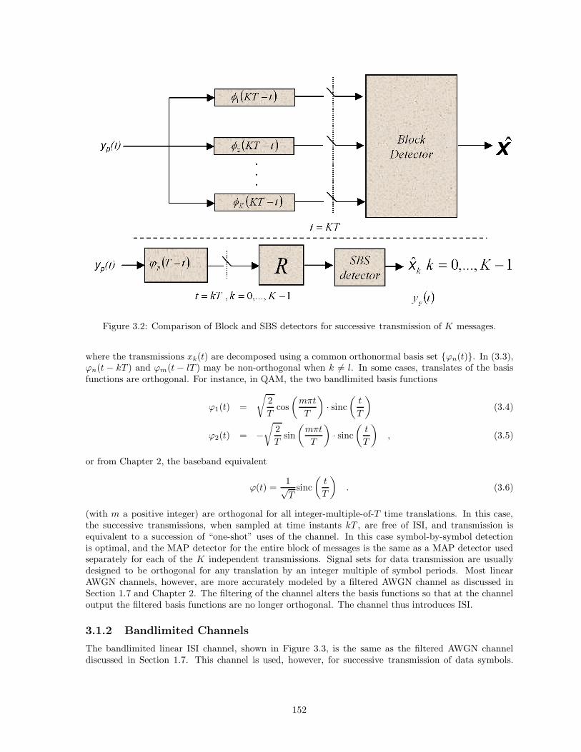
Figure 3.2: Comparison of Block and SBS detectors for successive transmission of K messages.
where the transmissions xk(t) are decomposed using a common orthonormal basis set {ϕn(t)}. In (3.3),ϕn(t − kT ) and ϕm(t − lT ) may be non-orthogonal when k 6= l. In some cases, translates of the basisfunctions are orthogonal. For instance, in QAM, the two bandlimited basis functions
ϕ1(t) =
√2T
cos(
mπt
T
)· sinc
(t
T
)(3.4)
ϕ2(t) = −√
2T
sin(
mπt
T
)· sinc
(t
T
), (3.5)
or from Chapter 2, the baseband equivalent
ϕ(t) =1√T
sinc(
t
T
). (3.6)
(with m a positive integer) are orthogonal for all integer-multiple-of-T time translations. In this case,the successive transmissions, when sampled at time instants kT , are free of ISI, and transmission isequivalent to a succession of “one-shot” uses of the channel. In this case symbol-by-symbol detectionis optimal, and the MAP detector for the entire block of messages is the same as a MAP detector usedseparately for each of the K independent transmissions. Signal sets for data transmission are usuallydesigned to be orthogonal for any translation by an integer multiple of symbol periods. Most linearAWGN channels, however, are more accurately modeled by a filtered AWGN channel as discussed inSection 1.7 and Chapter 2. The filtering of the channel alters the basis functions so that at the channeloutput the filtered basis functions are no longer orthogonal. The channel thus introduces ISI.
3.1.2 Bandlimited Channels
The bandlimited linear ISI channel, shown in Figure 3.3, is the same as the filtered AWGN channeldiscussed in Section 1.7. This channel is used, however, for successive transmission of data symbols.
152

Figure 3.3: The bandlimited channel, and equivalent forms with pulse response.
153

The (noise-free) channel output, xp(t), in Figure 3.3 is given by
xp(t) =K−1∑
k=0
N∑
n=1
xkn ·ϕn(t − kT ) ∗ h(t) (3.7)
=K−1∑
k=0
N∑
n=1
xkn · pn(t − kT ) (3.8)
where pn(t) ∆= ϕn(t) ∗ h(t). When h(t) 6= δ(t), the functions pn(t − kT ) do not necessarily form anorthonormal basis, nor are they even necessarily orthogonal. An optimum (MAP) detector would needto search a signal set of size MK , which is often too complex for implementation as K gets large. WhenN = 1 (or N = 2 with complex signals), there is only one pulse response p(t).
Equalization methods apply a processor, the “equalizer”, to the channel output to try to convert{pn(t − kT )} to an orthogonal set of functions. Symbol-by-symbol detection can then be used on theequalized channel output. Further discussion of such equalization filters is deferred to Section 3.4. Theremainder of this chapter also presumes that the channel-input symbol sequence xk is independent andidentically distributed at each point in time. This presumption will be relaxed in later Chapters.
While a very general theory of ISI could be undertaken for any N , such a theory would unnecessarilycomplicate the present development.2 This chapter handles the ISI-equalizer case for N = 1. Usingthe baseband-equivalent systems of Chapter 2, this chapter’s (Chapter 3’s) analysis will also apply toquadrature modulated systems modeled as complex (equivalent to two-dimensional real) channels. Inthis way, the developed theory of ISI and equalization will apply equally well to any one-dimensional(e.g. PAM) or two-dimensional (e.g. QAM or hexagonal) constellation. This was the main motivationfor the introduction of bandpass analysis in Chapter 2.
The pulse response for the transmitter/channel fundamentally quantifies ISI:
Definition 3.1.1 (Pulse Response) The pulse response of a bandlimited channel is de-fined by
p(t) = ϕ(t) ∗ h(t) . (3.9)
For the complex QAM case, p(t), ϕ(t), and h(t) can be complex time functions.
The one-dimensional noiseless channel output xp(t) is
xp(t) =K−1∑
k=0
xk · ϕ(t − kT ) ∗ h(t) (3.10)
=K−1∑
k=0
xk · p(t − kT ) . (3.11)
The signal in (3.11) is real for a one-dimensional system and complex for a baseband equivalent quadra-ture modulated system. The pulse response energy ‖p‖2 is not necessarily equal to 1, and this textintroduces the normalized pulse response:
ϕp(t)∆=
p(t)‖p‖
, (3.12)
where‖p‖2 =
∫ ∞
−∞p(t)p∗(t)dt = 〈p(t), p(t)〉 . (3.13)
The subscript p on ϕp(t) indicates that ϕp(t) is a normalized version of p(t). Using (3.12), Equation(3.11) becomes
xp(t) =K−1∑
k=0
xp,k · ϕp(t − kT ) , (3.14)
2Chapter 4 considers multidimensional signals and intersymbol interference, while Section 3.7 considers diversity re-ceivers that may have several observations a single or multiple channel output(s).
154

Figure 3.4: Illustration of intersymbol interference for p(t) = 11+t4 with T = 1.
wherexp,k
∆= xk · ‖p‖ . (3.15)
xp,k absorbs the channel gain/attenuation ‖p‖ into the definition of the input symbol, and thus hasenergy Ep = E
[|xp,k|2
]= Ex · ‖p‖2. While the functions ϕp(t − kT ) are normalized, they are not
necessarily orthogonal, so symbol-by-symbol detection is not necessarily optimal for the signal in (3.14).
EXAMPLE 3.1.1 (Intersymbol interference and the pulse response) As an exam-ple of intersymbol interference, consider the pulse response p(t) = 1
1+t4 and two successivetransmissions of opposite polarity (−1 followed by +1) through the corresponding channel.Figure 3.4 illustrates the two isolated pulses with correct polarity and also the waveformcorresponding to the two transmissions separated by 1 unit in time. Clearly the peaks of thepulses have been displaced in time and also significantly reduced in amplitude. Higher trans-mission rates would force successive transmissions to be closer and closer together. Figure3.5 illustrates the resultant sum of the two waveforms for spacings of 1 unit in time, .5 unitsin time, and .1 units in time. Clearly, ISI has the effect of severely reducing pulse strength,thereby reducing immunity to noise.
EXAMPLE 3.1.2 (Pulse Response Orthogonality - Modified Duobinary) A PAMmodulated signal using rectangular pulses is
ϕ(t) =1√T
(u(t) − u(t − T )) . (3.16)
The channel introduces ISI, for example, according to
h(t) = δ(t) + δ(t − T ). (3.17)
155

Figure 3.5: ISI with increasing symbol rate.
156

The resulting pulse response is
p(t) =1√T
(u(t) − u(t − 2T )) (3.18)
and the normalized pulse response is
ϕp(t) =1√2T
(u(t) − u(t − 2T )). (3.19)
The pulse-response translates ϕp(t) and ϕp(t− T ) are not orthogonal, even though ϕ(t) andϕ(t − T ) were originally orthonormal.
Noise Equivalent Pulse Response
Figure 3.6 models a channel with additive Gaussian noise that is not white, which often occurs in practice.The power spectral density of the noise is N0
2 · Sn(f). When Sn(f) 6= 0 (noise is never exactly zero atany frequency in practice), the noise psd has an invertible square root as in Section 1.7. The invertiblesquare-root can be realized as a filter in the beginning of a receiver. Since this filter is invertible, bythe reversibility theorem of Chapter 1, no information is lost. The designer can then construe this filteras being pushed back into, and thus a part of, the channel as shown in the lower part of Figure 3.6.The noise equivalent pulse response then has Fourier Transform P (f)/S
1/2n (f) for an equivalent filtered-
AWGN channel. The concept of noise equivalence allows an analysis for AWGN to be valid (using theequivalent pulse response instead of the original pulse response). Then also “colored noise” is equivalentin its effect to ISI, and furthermore the compensating equalizers that are developed later in this chaptercan also be very useful on channels that originally have no ISI, but that do have “colored noise.” AnAWGN channel with a notch in H(f) at some frequency is thus equivalent to a “flat channel” withH(f) = 1, but with narrow-band Gaussian noise at the same frequency as the notch.
3.1.3 The ISI-Channel Model
A model for linear ISI channels is shown in Figure 3.7. In this model, xk is scaled by ‖p‖ to form xp,k
so that Exp = Ex · ‖p‖2. The additive noise is white Gaussian, although correlated Gaussian noise canbe included by transforming the correlated-Gaussian-noise channel into an equivalent white Gaussiannoise channel using the methods in the previous subsection and illustrated in Figure 3.6. The channeloutput yp(t) is passed through a matched filter ϕ∗
p(−t) to generate y(t). Then, y(t) is sampled at thesymbol rate and subsequently processed by a discrete time receiver. The following theorem illustratesthat there is no loss in performance that is incurred via the matched-filter/sampler combination.
Theorem 3.1.1 (ISI-Channel Model Sufficiency) The discrete-time signal samples yk =y(kT ) in Figure 3.7 are sufficient to represent the continuous-time ISI-model channel outputy(t), if 0 < ‖p‖ < ∞. (i.e., a receiver with minimum Pe can be designed that uses only thesamples yk).
Sketch of Proof:Define
ϕp,k(t) ∆= ϕp(t − kT ) , (3.20)
where {ϕp,k(t)}k∈(−∞,∞) is a linearly independent set of functions. The set {ϕp,k(t)}k∈(−∞,∞)
is related to a set of orthogonal basis functions {φp,k(t)}k∈(−∞,∞) by an invertible transfor-mation Γ (use Gram-Schmidt an infinite number of times). The transformation and itsinverse are written
{φp,k(t)}k∈(−∞,∞) = Γ({ϕp,k(t)}k∈(−∞,∞)) (3.21)
{ϕp,k(t)}k∈(−∞,∞) = Γ−1({φp,k(t)}k∈(−∞,∞)) , (3.22)
where Γ is the invertible transformation. In Figure 3.8, the transformation outputs arethe filter samples y(kT ). The infinite set of filters {φ∗
p,k(−t)}k∈(−∞,∞) followed by Γ−1 is
157

Figure 3.6: White Noise Equivalent Channel.
Figure 3.7: The ISI-Channel model.
158

Figure 3.8: Equivalent diagram of ISI-channel model matched-filter/sampler
equivalent to an infinite set of matched filters to{
ϕ∗p,k(−t)
}k∈(−∞,∞)
. By (3.20) this last set
is equivalent to a single matched filter ϕ∗p(−t), whose output is sampled at t = kT to produce
y(kT ). Since the set {φp,k(t)}k∈(−∞,∞) is orthonormal, the set of sampled filter outputs inFigure 3.8 are sufficient to represent yp(t). Since Γ−1 is invertible (inverse is Γ), then by thetheorem of reversibility in Chapter 1, the sampled matched filter output y(kT ) is a sufficientrepresentation of the ISI-channel output yp(t). QED.
Referring to Figure 3.7,
y(t) =∑
k
‖p‖ · xkq(t − kT ) + np(t) ∗ ϕ∗p(−t) , (3.23)
whereq(t) ∆= ϕp(t) ∗ ϕ∗
p(−t) =p(t) ∗ p∗(−t)
‖p‖2. (3.24)
The deterministic autocorrelation function q(t) is Hermitian (q∗(−t) = q(t)). Also, q(0) = 1, so thesymbol xk passes at time kT to the output with amplitude scaling ‖p‖. The function q(t) can also exhibitISI, as illustrated in Figure 3.9. The plotted q(t) corresponds to qk = [−.1159 .2029 1 .2029 − .1159] or,
equivalently, to the channel p(t) =√
1T · (sinc(t/T ) + .25 · sinc((t − T )/T ) − .125 · sinc((t − 2T )/T )), or
159

Figure 3.9: ISI in q(t)
P (D) = 1√T· (1 + .5D)(1 − .25D) (the notation P (D) is defined in Appendix A.2). (The values for qk
can be confirmed by convolving p(t) with its time reverse, normalizing, and sampling.) For notationalbrevity, let yk
∆= y(kT ), qk∆= q(kT ), nk
∆= n(kT ) where n(t) ∆= np(t) ∗ ϕ∗p(−t). Thus
yk = ‖p‖ · xk︸ ︷︷ ︸scaled input (desired)
+ nk︸︷︷︸noise
+ ‖p‖ ·∑
m 6=k
xmqk−m
︸ ︷︷ ︸ISI
. (3.25)
The output yk consists of the scaled input, noise and ISI. The scaled input is the desired information-bearing signal. The ISI and noise are unwanted signals that act to distort the information being trans-mitted. The ISI represents a new distortion component not previously considered in the analysis ofChapters 1 and 2 for a suboptimum SBS detector. This SBS detector is the same detector as in Chap-ters 1 and 2, except used under the (false) assumption that the ISI is just additional AWGN. Such areceiver can be decidedly suboptimum when the ISI is nonzero.
Using D-transform notation, (3.25) becomes
Y (D) = X(D) · ‖p‖ · Q(D) + N (D) (3.26)
where Y (D) ∆=∑∞
k=−∞ yk ·Dk. If the receiver uses symbol-by-symbol detection on the sampled outputyk, then the noise sample nk of (one-dimensional) variance N0
2 at the matched-filter output combineswith ISI from the sample times mT (m 6= k) in corrupting ‖p‖ · xk.
There are two common measures of ISI distortion. The first is Peak Distortion, which only hasmeaning for real-valued q(t): 3
Definition 3.1.2 (Peak Distortion Criterion) If |xmax| is the maximum value for |xk|,then the peak distortion is:
Dp∆= |x|max · ‖p‖ ·
∑
m 6=0
|qm| . (3.27)
3In the real case, the magnitudes correspond to actual values. However, for complex-valued terms, the ISI is charac-terized by both its magnitude and phase. So, addition of the magnitudes of the symbols ignores the phase components,which may significantly change the ISI term.
160

For q(t) in Figure 3.9 with xmax = 3, Dp = 3·‖p‖(.1159+.2029+.2029+.1159) ≈ 3·√
1.078·.6376 ≈ 1.99.The peak distortion represents a worst-case loss in minimum distance between signal points in the
signal constellation for xk, or equivalently
Pe ≤ NeQ
‖p‖
dmin2 − Dp
σ
, (3.28)
for symbol-by-symbol detection. Consider two matched filter outputs yk and y′k that the receiver at-tempts to distinguish by suboptimally using symbol-by-symbol detection. These outputs are generatedby two different sequences {xk} and {x′
k}. Without loss of generality, assume yk > y′k, and consider thedifference
yk − y′k = ‖p‖
(xk − x′
k) +∑
m 6=k
(xm − x′m)qk−m
+ n (3.29)
The summation term inside the brackets in (3.29) represents the change in distance between yk and y′kcaused by ISI. Without ISI the distance is
yk − y′k ≥ ‖p‖ · dmin , (3.30)
while with ISI the distance can decrease to
yk − y′k ≥ ‖p‖
dmin − 2|x|max
∑
m 6=0
|qm|
. (3.31)
Implicitly, the distance interpretation in (3.31) assumes 2Dp ≤ ‖p‖dmin.4
While peak distortion represents the worst-case ISI, this worst case might not occur very often inpractice. For instance, with an input alphabet size M = 4 and a q(t) that spans 15 symbol periods,the probability of occurrence of the worst-case value (worst level occurring in all 14 ISI contributors) is4−14 = 3.7×10⁻⁹, well below typical channel Pe’s in data transmission. Nevertheless, there may be otherISI patterns of nearly just as bad interference that can also occur. Rather than separately compute eachpossible combination’s reduction of minimum distance, its probability of occurrence, and the resultingerror probability, data transmission engineers more often use a measure of ISI called Mean-SquareDistortion (valid for 1 or 2 dimensions):
Definition 3.1.3 (Mean-Square Distortion) The Mean-Square Distortion is definedby:
Dms∆= E
|∑
m 6=k
xp,m · qk−m|2 (3.32)
= Ex · ‖p‖2 ·∑
m 6=0
|qm|2 , (3.33)
where (3.33) is valid when the successive data symbols are independent and identically dis-tributed with zero mean.
In the example of Figure 3.9, the mean-square distortion (with Ex = 5) is Dms = 5‖p‖2(.11592+ .20292+.20292 + .11592) ≈ 5(1.078).109 ≈ .588. The fact
√.588 = .767 < 1.99 illustrates that Dms ≤ D2
p. (Theproof of this fact is left as an exercise to the reader.)
The mean-square distortion criterion assumes (erroneously5) that Dms is the variance of an uncor-related Gaussian noise that is added to nk. With this assumption, Pe is approximated by
Pe ≈ Ne ·Q
[‖p‖dmin
2√
σ2 + Dms
]. (3.34)
4On channels for which 2Dp ≥ ‖p‖dmin, the worst-case ISI occurs when |2Dp − ‖p‖dmin| is maximum.5This assumption is only true when xk is Gaussian. In very well-designeddata transmission systems, xk is approximately
i.i.d. and Gaussian, see Chapter 6, so that this approximation of Gaussian ISI becomes accurate.
161

One way to visualize ISI is through the “eye diagram”, some examples of which are shown in Figures3.10 and 3.11. The eye diagram is similar to what would be observed on an oscilloscope, when the triggeris synchronized to the symbol rate. The eye diagram is produced by overlaying several successive symbolintervals of the modulated and filtered continuous-time waveform (except Figures 3.10 and 3.11 do notinclude noise). The Lorentzian pulse response p(t) = 1/(1 + (3t/T )2) is used in both plots. For binarytransmission on this channel, there is a significant opening in the eye in the center of the plot in Figure3.10. With 4-level PAM transmission, the openings are much smaller, leading to less noise immunity.The ISI causes the spread among the path traces; more ISI results in a narrower eye opening. Clearlyincreasing M reduces the eye opening.
162

Figure 3.10: Binary eye diagram for a Lorentzian pulse response.
Figure 3.11: 4-Level eye diagram for a Lorentzian pulse response.
163

Figure 3.12: Use of possibly suboptimal receiver to approximate/create an equivalent AWGN.
3.2 Basics of the Receiver-generated Equivalent AWGN
Figure 3.12 focuses upon the receiver and specifically the device shown generally as R. When channelshave ISI, such a receiving device is inserted at the sampler output. The purpose of the receiver is toattempt to convert the channel into an equivalent AWGN that is also shown below the dashed line. Suchan AWGN is not always exactly achieved, but nonetheless any deviation between the receiver output zk
and the channel input symbol xk is viewed as additive white Gaussian noise. An SNR, as in Subsection3.2.1 can be used then to analyze the performance of the symbol-by-symbol detector that follows thereceiver R. Usually, smaller deviation from the transmitted symbol means better performance, althoughnot exactly so as Subsection 3.2.2 discusses. Subsection 3.2.3 finishes this section with a discussion ofthe highest possible SNR that a designer could expect for any filtered AWGN channel, the so-called“matched-filter-bound” SNR, SNRMFB. This section shall not be specific as to the content of the boxshown as R, but later sections will allow both linear and slightly nonlinear structures that may often begood choices because their performance can be close to SNRMFB .
3.2.1 Receiver Signal-to-Noise Ratio
Definition 3.2.1 (Receiver SNR) The receiver SNR, SNRR for any receiver R with(pre-decision) output zk, and decision regions based on xk (see Figure 3.12) is
SNRR∆=
ExE|ek|2
, (3.35)
where ek∆= xk − zk is the receiver error. The denominator of (3.35) is the mean-square
error MSE=E|ek|2. When E [zk|xk] = xk, the receiver is unbiased (otherwise biased) withrespect to the decision regions for xk.
The concept of a receiver SNR facilitates evaluation of the performance of data transmission systemswith various compensation methods (i.e. equalizers) for ISI. Use of SNR as a performance measurebuilds upon the simplifications of considering mean-square distortion, that is both noise and ISI arejointly considered in a single measure. The two right-most terms in (3.25) have normalized mean-squarevalue σ2 + Dms. The SNR for the matched filter output yk in Figure 3.12 is the ratio of channel outputsample energy Ex‖p‖2 to the mean-square distortion σ2 + Dms. This SNR is often directly related toprobability of error and is a function of both the receiver and the decision regions for the SBS detector.This text uses SNR consistently, replacing probability of error as a measure of comparative performance.SNR is easier to compute than Pe, independent of M at constant Ex, and a generally good measure
164

Figure 3.13: Receiver SNR concept.
of performance: higher SNR means lower probability of error. The probability of error is difficult tocompute exactly because the distribution of the ISI-plus-noise is not known or is difficult to compute.The SNR is easier to compute and this text assumes that the insertion of the appropriately scaled SNR(see Chapter 1 - Sections 1.4 - 1.6)) into the argument of the Q-function approximates the probability oferror for the suboptimum SBS detector. Even when this insertion into the Q-function is not sufficientlyaccurate, comparison of SNR’s for different receivers usually relates which receiver is better.
3.2.2 Receiver Biases
Figure 3.13 illustrates a receiver that somehow has tried to reduce the combination of ISI and noise.Any time-invariant receiver’s output samples, zk, satisfy
zk = α · (xk + uk) (3.36)
where α is some positive scale factor that may have been introduced by the receiver and uk is anuncorrelated distortion
uk =∑
m 6=0
rm · xk−m +∑
m
fm · nk−m . (3.37)
The coefficients for residual intersymbol interference rm and the coefficients of the filtered noise fk willdepend on the receiver and generally determine the level of mean-square distortion. The uncorrelateddistortion has no remnant of the current symbol being decided by the SBS detector, so that E [uk/xk] = 0.However, the receiver may have found that by scaling (reducing) the xk component in zk by α thatthe SNR improves (small signal loss in exchange for larger uncorrelated distortion reduction). WhenE [zk/xk] = α · xk 6= xk, the decision regions in the SBS detector are “biased.” Removal of the bias iseasily achieved by scaling by 1/α as also in Figure 3.13. If the distortion is assumed to be Gaussiannoise, as is the assumption with the SBS detector, then removal of bias by scaling by 1/α improves theprobability of error of such a detector as in Chapter 1. (Even when the noise is not Gaussian as is thecase with the ISI component, scaling the signal correctly improves the probability of error on the averageif the input constellation has zero mean.)
The following theorem relates the SNR’s of the unbiased and biased decision rules for any receiverR:
Theorem 3.2.1 (Unconstrained and Unbiased Receivers) Given an unbiased receiverR for a decision rule based on a signal constellation corresponding to xk, the maximumunconstrained SNR corresponding to that same receiver with any biased decision rule is
SNRR = SNRR,U + 1 , (3.38)
165

where SNRR,U is the SNR using the unbiased decision rule.
Proof: From Figure 3.13, the SNR after scaling is easily
SNRR,U =Exσ2
u
. (3.39)
The maximum SNR for the biased signal zk prior to the scaling occurs when α is chosen to maximizethe unconstrained SNR
SNRR =Ex
|α|2σ2u + |1− α|2Ex
. (3.40)
Allowing for complex α with phase θ and magnitude |α|, the SNR maximization over alpha is equivalentto minimizing
1 − 2|α|cos(θ) + |α|2(1 +1
SNRR,U) . (3.41)
Clearly θ = 0 for a minimum and differentiating with respect to |α| yields −2 + 2|α|(1 + 1SNRR,U
) = 0
or αopt = 1/(1 + (SNRR,U )−1). Substitution of this value into the expression for SNRR finds
SNRR = SNRR,U + 1 . (3.42)
Thus, a receiver R and a corresponding SBS detector that have zero bias will not correspond to a max-imum SNR – the SNR can be improved by scaling (reducing) the receiver output by αopt. Conversely,a receiver designed for maximum SNR can be altered slightly through simple output scaling by 1/αopt
to a related receiver that has no bias and has SNR thereby reduced to SNRR,U = SNRR − 1. QED.
To illustrate the relationship of unbiased and biased receiver SNRs, suppose an ISI-free AWGNchannel has an SNR=10 with Ex = 1 and σ2
u = N02
= .1. Then, a receiver could scale the channel outputby α = 10/11. The resultant new error signal is ek = xk(1 − 10
11) − 10
11nk, which has MSE=E[|ek|2] =
1121 + 100
121(.1) = 111 , and SNR=11. Clearly, the biased SNR is equal to the unbiased SNR plus 1. The
scaling has done nothing to improve the system, and the appearance of an improved SNR is an artifactof the SNR definition, which allows noise to be scaled down without taking into account the fact thatactual signal power after scaling has also been reduced. Removing the bias corresponds to using theactual signal power, and the corresponding performance-characterizing SNR can always be found bysubtracting 1 from the biased SNR. A natural question is then “Why compute the biased SNR?” Theanswer is that the biased receiver corresponds directly to minimizing the mean-square distortion, andthe SNR for the “MMSE” case will often be easier to compute. Figure 3.27 in Section 3.5 illustratesthe usual situation of removing a bias (and consequently reducing SNR, but not improving Pe since theSBS detector works best when there is no bias) from a receiver that minimizes mean-square distortion(or error) to get an unbiased decision. The bias from a receiver that maximizes SNR by equivalentlyminimizing mean-square error can then be removed by simple scaling and the resultant more accurateSNR is thus found for the unbiased receiver by subtracting 1 from the more easily computed biasedreceiver. This concept will be very useful in evaluating equalizer performance in later sections of thischapter, and is formalized in Theorem 3.2.2 below.
Theorem 3.2.2 (Unbiased MMSE Receiver Theorem) Let R be any allowed class ofreceivers R producing outputs zk, and let Ropt be the receiver that achieves the maximumsignal-to-noise ratio SNR(Ropt) over all R ∈ R with an unconstrained decision rule. Thenthe receiver that achieves the maximum SNR with an unbiased decision rule is also Ropt, and
maxR∈R
SNRR,U = SNR(Ropt) − 1. (3.43)
Proof. From Theorem 3.2.1, for any R ∈ R, the relation between the signal-to-noise ratios of unbiasedand unconstrained decision rules is SNRR,U = SNRR − 1, so
maxR∈R
[SNRR,U ] = maxR∈R
[SNRR]− 1 = SNRRopt − 1 . (3.44)
166

QED.This theorem implies that the optimum unbiased receiver and the optimum biased receiver settings
are identical except for any scaling to remove bias; only the SNR measures are different. For any SBSdetector, SNRR,U is the SNR that corresponds to best Pe. The quantity SNRR,U + 1 is artificially highbecause of the bias inherent in the general SNR definition.
3.2.3 The Matched-Filter Bound
The Matched-Filter Bound (MFB), also called the “one-shot” bound, specifies an upper SNR limiton the performance of data transmission systems with ISI.
Lemma 3.2.1 (Matched-Filter Bound SNR) The SNRMFB is the SNR that character-izes the best achievable performance for a given pulse response p(t) and signal constellation(on an AWGN channel) if the channel is used to transmit only one message. This SNR is
SNRMFB =Ex‖p‖2
N02
(3.45)
MFB denotes the square of the argument to the Q-function that arises in the equivalent“one-shot” analysis of the channel.
Proof: Given a channel with pulse response p(t) and isolated input x0, the maximum output sampleof the matched filter is ‖p‖ · x0. The normalized average energy of this sample is ‖p‖2Ex, while thecorresponding noise sample energy is N0
2, SNRMFB = Ex‖p‖2
N02
. QED.
The probability of error, measured after the matched filter and prior to the symbol-by-symbol detector,satisfies Pe ≥ Ne ·Q(
√MFB). When Ex equals (d2
min/4)/κ, then MFB equals SNRMFB ·κ. In effect theMFB forces no ISI by disallowing preceding or successive transmitted symbols. An optimum detector isused for this “one-shot” case. The performance is tacitly a function of the transmitter basis functions,implying performance is also a function of the symbol rate 1/T . No other (for the same input constel-lation) receiver for continuous transmission could have better performance, if xk is an i.i.d. sequence,since the sequence must incur some level of ISI. The possibility of correlating the input sequence {xk}to take advantage of the channel correlation will be considered in Chapters 4 and 5.
The following example illustrates computation of the MFB for several cases of practical interest:
EXAMPLE 3.2.1 (Binary PAM) For binary PAM,
xp(t) =∑
k
xk · p(t − kT ) , (3.46)
where xk = ±√Ex. The minimum distance at the matched-filter output is ‖p‖ · dmin =
‖p‖ · d = 2 · ‖p‖ ·√Ex, so Ex =
d2
min4
and κ = 1. Then,
MFB = SNRMFB . (3.47)
Thus for a binary PAM channel, the MFB (in dB) is just the “channel-output” SNR,SNRMFB. If the transmitter symbols xk are equal to ±1 (Ex = 1), then
MFB =‖p‖2
σ2, (3.48)
where, again, σ2 = N02 . The binary-PAM Pe is then bounded by
Pe ≥ Q(√
SNRMFB) . (3.49)
167

EXAMPLE 3.2.2 (M-ary PAM) For M-ary PAM, xk = ±d2 , ±3d
2 , ..., ± (M−1)d2 and
d
2=
√3Ex
M2 − 1, (3.50)
so κ = 3/(M2 − 1). Thus,
MFB =3
M2 − 1SNRMFB , (3.51)
for M ≥ 2. If the transmitter symbols xk are equal to ±1,±3, , ..., ±(M − 1), then
MFB =‖p‖2
σ2. (3.52)
Equation (3.52) is the same result as (3.48), which should be expected since the minimumdistance is the same at the transmitter, and thus also at the channel output, for both (3.48)and (3.52). The M’ary-PAM Pe is then bounded by
Pe ≥ 2(1 − 1/M ) · Q(
√3 · SNRMFB
M2 − 1) . (3.53)
EXAMPLE 3.2.3 (QPSK) For QPSK, xk = ±d2± d
2, and d = 2
√Ex, so κ = 1. Thus
MFB = SNRMFB . (3.54)
Thus, for a QPSK (or 4SQ QAM) channel, MFB (in dB) equals the channel output SNR. Ifthe transmitter symbols xk are ±1 ± , then
MFB =‖p‖2
σ2. (3.55)
The best QPSK Pe is then approximated by
Pe ≈ Q(√
SNRMFB) . (3.56)
EXAMPLE 3.2.4 (M-ary QAM Square) For M-ary QAM, <{xk} = ±d2, ±3d
2, ..., ± (
√M−1)d
2,
={xk} = ±d2, ±3d
2, ..., ± (
√M−1)d
2, (recall that < and = denote real and imaginary parts,
respectively) and
d
2=
√3Ex
M − 1, (3.57)
so κ = 3/(M − 1). Thus
MFB =3
M − 1SNRMFB , (3.58)
for M ≥ 4. If the real and imaginary components of the transmitter symbols xk equal±1,±3, , ..., ±(
√M − 1), then
MFB =‖p‖2
σ2. (3.59)
The best M’ary QAM Pe is then approximated by
Pe ≈ 2(1 − 1/√
M) · Q(
√3 · SNRMFB
M − 1) . (3.60)
168

In general for square QAM constellations,
MFB =3
4b − 1SNRMFB . (3.61)
For the QAM Cross constellations,
MFB =
2Ex‖p‖2
3148 M− 2
3
σ2=
9631 · 4b − 32
SNRMFB . (3.62)
For the suboptimum receivers to come in later sections, SNRU ≤ SNRMFB . As SNRU → SNRMFB,then the receiver is approaching the bound on performance. It is not always possible to design a receiverthat attains SNRMFB , even with infinite complexity, unless one allows co-design of the input symbolsxk in a channel-dependent way (see Chapters 4 and 5). The loss with respect to matched filter boundwill be determined for any receiver by SNRu/SNRMFB ≤ 1, in effect determining a loss in signal powerbecause successive transmissions interfere with one another – it may well be that the loss in signal poweris an acceptable exchange for a higher rate of transmission.
169

3.3 Nyquist’s Criterion
Nyquist’s Criterion specifies the conditions on q(t) = ϕp(t) ∗ ϕ∗p(−t) for an ISI-free channel on which a
symbol-by-symbol detector is optimal. This section first reviews some fundamental relationships betweenq(t) and its samples qk = q(kT ) in the frequency domain.
q(kT ) =12π
∫ ∞
−∞Q(ω)eωkT dω (3.63)
=12π
∞∑
n=−∞
∫ (2n+1)πT
(2n−1)πT
Q(ω)eωkT dω (3.64)
=12π
∞∑
n=−∞
∫ πT
− πT
Q(ω +2πn
T)e(ω+ 2πn
T )kTdω (3.65)
=12π
∫ πT
− πT
Qeq(ω)eωkT dω , (3.66)
where Qeq(ω), the equivalent frequency response becomes
Qeq(ω) ∆=∞∑
n=−∞Q(ω +
2πn
T) . (3.67)
The function Qeq(ω) is periodic in ω with period 2πT . This function is also known as the folded or aliased
spectrum of Q(ω) because the sampling process causes the frequency response outside of the fundamentalinterval (− π
T , πT ) to be added (i.e. “folded in”). Writing the Fourier Transform of the sequence qk as
Q(e−ωT ) =∑∞
k=−∞ qke−ωkT leads to
1T
·Qeq(ω) = Q(e−ωT ) ∆=∞∑
k=−∞
qke−ωkT , (3.68)
a well-known relation between the discrete-time and continuous-time representations of any waveformin digital signal processing.
It is now straightforward to specify Nyquist’s Criterion:
Theorem 3.3.1 (Nyquist’s Criterion) A channel specified by pulse response p(t) (andresulting in q(t) = p(t)∗p∗(−t)
‖p‖2 ) is ISI-free if and only if
Q(e−ωT ) =1T
∞∑
n=−∞Q(ω +
2πn
T) = 1 . (3.69)
Proof:By definition the channel is ISI-free if and only if qk = 0 for all k 6= 0 (recall q0 = 1 bydefinition). The proof follows directly by substitution of qk = δk into (3.68). QED.
Functions that satisfy (3.69) are called “Nyquist pulses.” One function that satisfies Nyquist’sCriterion is
q(t) = sinc(
t
T
), (3.70)
which corresponds to normalized pulse response
ϕp(t) =1√T
sinc(
t
T
). (3.71)
The function q(kT ) = sinc(k) = δk satisfies the ISI-free condition. One feature of sinc(t/T ) is that it hasminimum bandwidth for no ISI. No other function has this same minimum bandwidth and also satisfies
170

Figure 3.14: The sinc(t/T) function.
the Nyquist Criterion. (Proof is left as an exercise to the reader.) The sinc(t/T ) function is plotted inFigure 3.14 for −20T ≤ t ≤ 20T .
The frequency 12T
(1/2 the symbol rate) is often construed as the maximum frequency of a sampledsignal that can be represented by samples at the sampling rate. In terms of positive-frequencies, 1/2Trepresents a minimum bandwidth necessary to satisfy the Nyquist Criterion, and thus has a special namein data transmission:
Definition 3.3.1 (Nyquist Frequency) The frequency ω = πT or f = 1
2T is called theNyquist frequency.6
3.3.1 Vestigial Symmetry
In addition to the sinc(t/T ) Nyquist pulse, data-transmission engineers use responses with up to twicethe minimum bandwidth. For all these pulses, Q(ω) = 0 for |ω| > 2π
T. These wider bandwidth responses
will provide more immunity to timing errors in sampling as follows: The sinc(t/T ) function decays inamplitude only linearly with time. Thus, any sampling-phase error in the sampling process of Figure 3.7introduces residual ISI with amplitude that only decays linearly with time. In fact for q(t) = sinc(t/T ),the ISI term
∑k 6=0 q(τ +kT ) with a sampling timing error of τ 6= 0 is not absolutely summable, resulting
in infinite peak distortion. The envelope of the time domain response decays more rapidly if the frequencyresponse is smooth (i.e. continuously differentiable). To meet this smoothness condition and also satisfyNyquist’s Criterion, the response must occupy a larger than minimum bandwidth that is between 1/2Tand 1/T . A q(t) with higher bandwidth can exhibit significantly faster decay as |t| increases, thusreducing sensitivity to timing phase errors. Of course, any increase in bandwidth should be as small aspossible, while still meeting other system requirements. The percent excess bandwidth7, or percentroll-off, is a measure of the extra bandwidth.
Definition 3.3.2 (Percent Excess Bandwidth) The percent excess bandwidth α isdetermined from a strictly bandlimited Q(ω) by finding the highest frequency in Q(ω) for
6This text distinguishes the Nyquist Frequency from the Nyquist Rate in sampling theory, where the latter is twice thehighest frequency of a signal to be sampled and is not the same as the Nyquist Frequency here.
7The quantity alpha used here is not a bias factor, and similarly Q(·) is a measure of ISI and not the integral of aunit-variance Gaussian function – uses should be clear to reasonable readers who’ll understand that sometimes symbolsare re-used in obviously differenct contexts.
171

Figure 3.15: The sinc2(t/T ) Function – time-domain
which there is nonzero energy transfer. That is
Q(ω) ={
nonzero |ω| ≤ (1 + α) πT
0 |ω| > (1 + α) πT
.. (3.72)
Thus, if α = .15 (a typical value), the pulse q(t) is said to have “15% excess bandwidth.” Usually, datatransmission systems have 0 ≤ α ≤ 1. In this case in equation (3.69), only the terms n = −1, 0, +1contribute to the folded spectrum and the Nyquist Criterion becomes
1 = Q(e−ωT ) (3.73)
=1T
{Q
(ω +
2π
T
)+ Q (ω) + Q
(ω − 2π
T
)}− π
T≤ ω ≤ π
T. (3.74)
Further, recalling that q(t) = ϕp(t) ∗ ϕ∗p(−t) is Hermitian and has the properties of an autocorrelation
function, then Q(ω) is real and Q(ω) ≥ 0. For the region 0 ≤ ω ≤ πT (for real signals), (3.74) reduces to
1 = Q(e−ωT ) (3.75)
=1T
{Q (ω) + Q
(ω −
2π
T
)}. (3.76)
For complex signals, the negative frequency region (− πT≤ ω ≤ 0) should also have
1 = Q(e−ωT ) (3.77)
=1T
{Q (ω) + Q
(ω +
2π
T
)}. (3.78)
Any Q(ω) satisfying (3.76) (and (3.78) in the complex case) is said to be vestigially symmetricwith respect to the Nyquist Frequency. An example of a vestigially symmetric response with 100% excessbandwidth is q(t) = sinc2(t/T ), which is shown in Figures 3.15 and 3.16.
3.3.2 Raised Cosine Pulses
The most widely used set of functions that satisfy the Nyquist Criterion are the raised-cosine pulseshapes:
172

Figure 3.16: The sinc2(t/T ) function – frequency-domain
Figure 3.17: Raised cosine pulse shapes – time-domain
173

Figure 3.18: Raised Cosine Pulse Shapes – frequency-domain
Definition 3.3.3 (Raised-Cosine Pulse Shapes) The raised cosine family of pulse shapes(indexed by 0 ≤ α ≤ 1) is given by
q(t) = sinc(
t
T
)·
[cos(
απtT
)
1 −(
2αtT
)2
], (3.79)
and have Fourier Transforms
Q(ω) =
T |ω| ≤ πT (1 − α)
T2
[1 − sin
(T2α(|ω| − π
T ))]
πT (1 − α) ≤ |ω| ≤ π
T (1 + α)0 π
T (1 + α) ≤ |ω|. (3.80)
The raised cosine pulse shapes are shown in Figure 3.17 (time-domain) and Figure 3.18 (frequency-domain) for α = 0, .5, and 1. When α = 0, the raised cosine reduces to a sinc function, which decaysasymptotically as 1
t for t → ∞, while for α 6= 0, the function decays as 1t3 for t → ∞.
3.3.3 Square-Root Splitting of the Nyquist Pulse
The optimum ISI-free transmission system that this section has described has transmit-and-channelfiltering ϕp(t) and receiver matched filter ϕ∗
p(−t) such that q(t) = ϕp(t) ∗ϕ∗p(−t) or equivalently
Φp(ω) = Q1/2(ω) (3.81)
so that the matched filter and transmit/channel filters are “square-roots” of the Nyquist pulse. Whenh(t) = δ(t) or equivalently ϕp(t) = ϕ(t) , the transmit filter (and the receiver matched filters) are square-roots of a Nyquist pulse shape. Such square-root transmit filtering is often used even when ϕp(t) 6= ϕ(t)and the pulse response is the convolution of h(t) with the square-root filter.
The raised-cosine pulse shapes are then often used in square-root form, which is
√Q(ω) =
√T |ω| ≤ π
T (1 − α)√T2
[1 − sin
(T2α
(|ω| − πT
))]1/2 π
T(1 − α) ≤ |ω| ≤ π
T(1 + α)
0 πT (1 + α) ≤ |ω|
. (3.82)
174

This expression can be inverted to the time-domain via use of the identity sin2(θ) = .5(1− cos(2θ)), asin the exercises, to obtain
ϕp(t) =4α
π√
T·cos([1 + α]πt
T
)+
T ·sin([1−α] πtT )
4αt
1 −(
4αtT
)2 . (3.83)
175

3.4 Linear Zero-Forcing Equalization
This section examines the Zero-Forcing Equalizer (ZFE), which is the easiest type of equalizer toanalyze and understand, but has inferior performance to some other equalizers to be introduced in latersections. The ISI model in Figure 3.7 is used to describe the zero-forcing version of the discrete-timereceiver. The ZFE is often a first non-trivial attempt at a receiver R in Figure 3.12 of Section 3.2.
The ZFE sets R equal to a linear time-invariant filter with discrete impulse response wk that actson yk to produce zk, which is an estimate of xk. Ideally, for symbol-by-symbol detection to be optimal,qk = δk by Nyquist’s Criterion. The equalizer tries to restore this Nyquist Pulse character to thechannel. In so doing, the ZFE ignores the noise and shapes the signal yk so that it is free of ISI. Fromthe ISI-channel model of Section 3.1 and Figure 3.7,
yk = ‖p‖ · xk ∗ qk + nk . (3.84)
In the ZFE case, nk is initially viewed as being zero. The D-transform of yk is (See Appendix A.2)
Y (D) = ‖p‖ · X(D) ·Q(D) . (3.85)
The ZFE output, zk, has Transform
Z(D) = W (D) · Y (D) = W (D) ·Q(D) · ‖p‖ ·X(D) , (3.86)
and will be free of ISI if Z(D) = X(D), leaving the ZFE filter characteristic:
Definition 3.4.1 (Zero-Forcing Equalizer) The ZFE transfer characteristic is
W (D) =1
Q(D) · ‖p‖. (3.87)
This discrete-time filter processes the discrete-time sequence corresponding to the matched-filter output.The ZFE is so named because ISI is “forced to zero” at all sampling instants kT except k = 0. Thereceiver uses symbol-by-symbol detection, based on decision regions for the constellation defined by xk,on the output of the ZFE.
3.4.1 Performance Analysis of the ZFE
The variance of the noise, which is not zero in practice, at the output of the ZFE is important indetermining performance, even if ignored in the ZFE design of Equation (3.87). As this noise is producedby a linear filter acting on the discrete Gaussian noise process nk, it is also Gaussian. The designer cancompute the discrete autocorrelation function (the bar denotes normalized to one dimension, so N = 2for the complex QAM case) for the noise nk as
rnn,k = E[nln
∗l−k
]/N (3.88)
=∫ ∞
−∞
∫ ∞
−∞E[np(t)n∗
p(s)]ϕ∗
p(t − lT )ϕp(s − (l − k)T )dtds (3.89)
=∫ ∞
−∞
∫ ∞
−∞
N0
2δ(t − s)ϕ∗
p(t − lT )ϕp(s − (l − k)T )dtds (3.90)
=N0
2
∫ ∞
−∞ϕ∗
p(t − lT )ϕp(t − (l − k)T )dt (3.91)
=N0
2
∫ ∞
−∞ϕ∗
p(u)ϕp(u + kT )du (letting u = t − lT ) (3.92)
=N0
2q∗−k =
N0
2qk , (3.93)
or more simply
Rnn(D) =N0
2Q(D) , (3.94)
176

where the analysis uses the substitution u = t− lT in going from (3.91) to (3.92), and assumes basebandequivalent signals for the complex case. The complex baseband-equivalent noise, has (one-dimensional)sample variance N0
2 at the normalized matched filter output. The noise at the output of the ZFE,nZFE,k, has autocorrelation function
rZFE,k = rnn,k ∗ wk ∗ w∗−k . (3.95)
The D-Transform of rZFE,k is then
RZFE(D) =N0
2Q(D)
‖p‖2 · Q2(D)=
N02
‖p‖2 · Q(D). (3.96)
The power spectral density of the noise samples nZFE,k is then RZFE(e−ωT ). The (per-dimensional)variance of the noise samples at the output of the ZFE is the (per-dimensional) mean-square errorbetween the desired xk and the ZFE output zk. Since
zk = xk + nZFE,k , (3.97)
then σ2ZFE is computed as
σ2ZFE =
T
2π
∫ πT
− πT
RZFE(e−ωT )dω =T
2π
∫ πT
− πT
N02
‖p‖2 ·Q(e−ωT )dω =
N02
‖p‖2γZFE =
N02
‖p‖· w0 , (3.98)
where
γZFE =T
2π
∫ πT
− πT
1Q(e−ωT )
dω = w0 · ‖p‖ . (3.99)
The center tap of a linear equalizer is w0, or if the ZFE is explicity used, then wZFE,0. This tap iseasily shown to always have the largest magnitude for a ZFE and thus spotted readily when plotting theimpulse response of any linear equalizer. From (3.97) and the fact that E [nZFE,k] = 0, E [zk/xk] = xk,so that the ZFE is unbiased for a detection rule based on xk. The SNR at the output of the ZFE is
SNRZFE =Ex
σ2ZFE
= SNRMFB · 1γZFE
. (3.100)
Computation of dmin over the signal set corresponding to xk leads to a relation between Ex, dmin, andM , and the NNUB on error probability for a symbol-by-symbol detector at the ZFE output is (please,do not confuse the Q function with the channel autocorrelation Q(D))
PZFE,e ≈ Ne · Q(
dmin2σZFE
). (3.101)
Since symbol-by-symbol detection can never have performance that exceeds the MFB,
σ2 ≤ σ2ZFE‖p‖2 = σ2 T
2π
∫ πT
− πT
dω
Q(e−ωT )= σ2 · γZFE (3.102)
SNRMFB ≥ SNRZFE (3.103)γZFE ≥ 1 , (3.104)
with equality if and only if Q(D) = 1.Finally, the ZFE equalization loss, 1/γZFE , defines the SNR reduction from the MFB:
Definition 3.4.2 (ZFE Equalization Loss) The ZFE Equalization Loss, γZFE in deci-bels is
γZFE∆= 10 · log10
(SNRMFB
SNRZFE
)= 10 log10
‖p‖2 · σ2ZFE
σ2= 10 log10 ‖p‖ ·wZFE,0 , (3.105)
and is a measure of the loss (in dB) with respect to the MFB for the ZFE. The sign of theloss is often ignored since it is always a negative (or 0) number and only its magnitude is ofconcern.
Equation (3.105) always thus provides a non-negative number.
177

Figure 3.19: Noise Enhancement
3.4.2 Noise Enhancement
The design of W (D) for the ZFE ignored the effects of noise. This oversight can lead to noise enhance-ment, a σ2
ZFE that is unacceptably large, and the consequent poor performance.Figure 3.19 hypothetically illustrates an example of a lowpass channel with a notch at the Nyquist
Frequency, that is, Q(e−ωT ) is zero at ω = πT . Since W (e−ωT ) = 1/(‖p‖ · Q(e−ωT )), then any noise
energy near the Nyquist Frequency is enhanced (increased in power or energy), in this case so muchthat σ2
ZFE → ∞. Even when there is no channel notch at any frequency, σ2ZFE can be finite, but large,
leading to unacceptable performance degradation.In actual computation of examples, the author has found that the table in Table 3.1 is useful in
recalling basic digital signal processing equivalences related to scale factors between continuous timeconvolution and discrete-time convolution.
The following example clearly illustrates the noise-enhancement effect:
EXAMPLE 3.4.1 (1 + .9D−1 - ZFE) Suppose the pulse response of a (strictly bandlim-ited) channel used with binary PAM is
P (ω) ={ √
T(1 + .9eωT
)|ω| ≤ π
T0 |ω| > π
T
. (3.106)
Then ‖p‖2 is computed as
‖p‖2 =12π
∫ πT
− πT
|P (ω)|2dω (3.107)
=12π
∫ πT
− πT
T [1.81 + 1.8 cos(ωT )] dω (3.108)
=T
2π1.81
2π
T= 1.81 = 12 + .92 . (3.109)
The magnitude of the Fourier transform of the pulse response appears in Figure 3.20. Thus,with Φp(ω) as the Fourier transform of {ϕp(t)},
Φp(ω) =
{ √T
1.81
(1 + .9eωT
)|ω| ≤ π
T
0 |ω| > πT
. (3.110)
178

Table 3.1: Conversion factors of T .
179
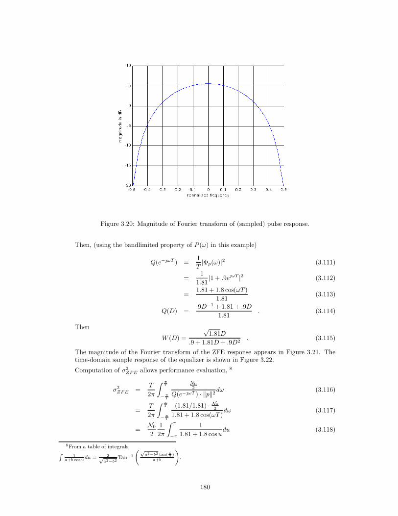
Figure 3.20: Magnitude of Fourier transform of (sampled) pulse response.
Then, (using the bandlimited property of P (ω) in this example)
Q(e−ωT ) =1T|Φp(ω)|2 (3.111)
=1
1.81|1 + .9eωT |2 (3.112)
=1.81 + 1.8 cos(ωT )
1.81(3.113)
Q(D) =.9D−1 + 1.81 + .9D
1.81. (3.114)
Then
W (D) =√
1.81D.9 + 1.81D + .9D2
. (3.115)
The magnitude of the Fourier transform of the ZFE response appears in Figure 3.21. Thetime-domain sample response of the equalizer is shown in Figure 3.22.
Computation of σ2ZFE allows performance evaluation, 8
σ2ZFE =
T
2π
∫ πT
− πT
N02
Q(e−ωT ) · ‖p‖2dω (3.116)
=T
2π
∫ πT
− πT
(1.81/1.81) · N02
1.81 + 1.8 cos(ωT )dω (3.117)
=N0
212π
∫ π
−π
11.81 + 1.8 cos u
du (3.118)
8From a table of integrals∫
1a+b cos u
du = 2√a2−b2
Tan−1
(√a2−b2 tan( u
2 )
a+b
).
180
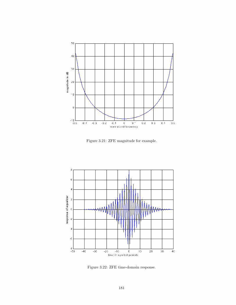
Figure 3.21: ZFE magnitude for example.
Figure 3.22: ZFE time-domain response.
181

= (N0
2)
22π
[2√
1.812 − 1.82Tan−1
√1.812 − 1.82 tan u
2
1.81 + 1.8
∣∣∣∣∣
π
0
(3.119)
= (N0
2)
42π
√1.812 − 1.82
·π
2(3.120)
= (N0
2)
1√1.812 − 1.82
(3.121)
=N0
2(5.26) . (3.122)
The ZFE-output SNR is
SNRZFE =Ex
5.26N02
. (3.123)
This SNRZFE is also the argument of the Q-function for a binary detector at the ZFE output.Assuming the two transmitted levels are xk = ±1, then we get
MFB =‖p‖2
σ2=
1.81σ2
, (3.124)
leavingγZFE = 10 log10(1.81 · 5.26) ≈ 9.8dB (3.125)
for any value of the noise variance. This is very poor performance on this channel. No matterwhat b is used, the loss is almost 10 dB from best performance. Thus, noise enhancementcan be a serious problem. Chapter 9 demonstrates a means by which to ensure that thereis no loss with respect to the matched filter bound for this channel. With alteration of thesignal constellation, Chapter 10 describes a means that ensures an error rate of 10−5 on thischannel, with no information rate loss, which is far below the error rate achievable even whenthe MFB is attained. thus, there are good solutions, but the simple concept of a ZFE is nota good solution.
Another example illustrates the generalization of the above procedure when the pulse response is complex(corresponding to a QAM channel):
EXAMPLE 3.4.2 (QAM: −.5D−1 + (1 + .25) − .5D Channel) Given a baseband equiv-alent channel
p(t) =1√T
{−
12sinc
(t + T
T
)+(1 +
4
)sinc
(t
T
)−
2sinc
(t − T
T
)}, (3.126)
the discrete-time channel samples are
pk =1√T
[−1
2,(1 +
4
), −
2
]. (3.127)
This channel has the transfer function of Figure 3.23. The pulse response norm (squared) is
‖p‖2 =T
T(.25 + 1 + .0625 + .25) = 1.5625 . (3.128)
Then qk is given by
qk = q(kT ) = T(ϕp,k ∗ ϕ∗
p,−k
)=
11.5625
[−
4,
58(−1 + ) , 1.5625 , −5
8(1 + ) ,
4
]
(3.129)or
Q(D) =1
1.5625
[−
4D−2 +
58(−1 + )D−1 + 1.5625− 5
8(1 + )D +
4D2
](3.130)
182

Figure 3.23: Fourier transform magnitude for pulse response for complex channel example.
Then, Q(D) factors into
Q(D) =1
1.5625{(1 − .5D)
(1 − .5D−1
) (1 + .5D−1
)(1 − .5D)
}, (3.131)
andWZFE(D) =
1Q(D)‖p‖
(3.132)
or
WZFE(D) =√
1.5625(−.25D−2 + .625(−1 + )D−1 + 1.5625− .625(1 + )D + .25D2)
. (3.133)
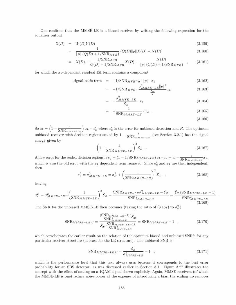
The Fourier transform of the ZFE is in Figure 3.24. The real and imaginary parts of theequalizer response in the time domain are shown in Figure 3.25 Then
σ2ZFE =
T
2π
∫ πT
− πT
N02
‖p‖2Q(e−ωT )dω , (3.134)
orσ2
ZFE =N0
2w0
‖p‖ , (3.135)
where w0 is the zero (center) coefficient of the ZFE. This coefficient can be extracted from
WZFE (D) =√
1.5625[
D2(−4){(D + 2) (D − 2) (D − .5) (D + .5)}
]
=√
1.5625[
A
D − 2+
B
D + 2+ terms not contributing to w0
],
where A and B are coefficients in the partial-fraction expansion (the residuez and residuecommands in Matlab can be very useful here):
A =4(−4)
(2 + 2)(2 + .5)(1.5)= −1.5686− .9412 = 1.82936 − 2.601 (3.136)
183
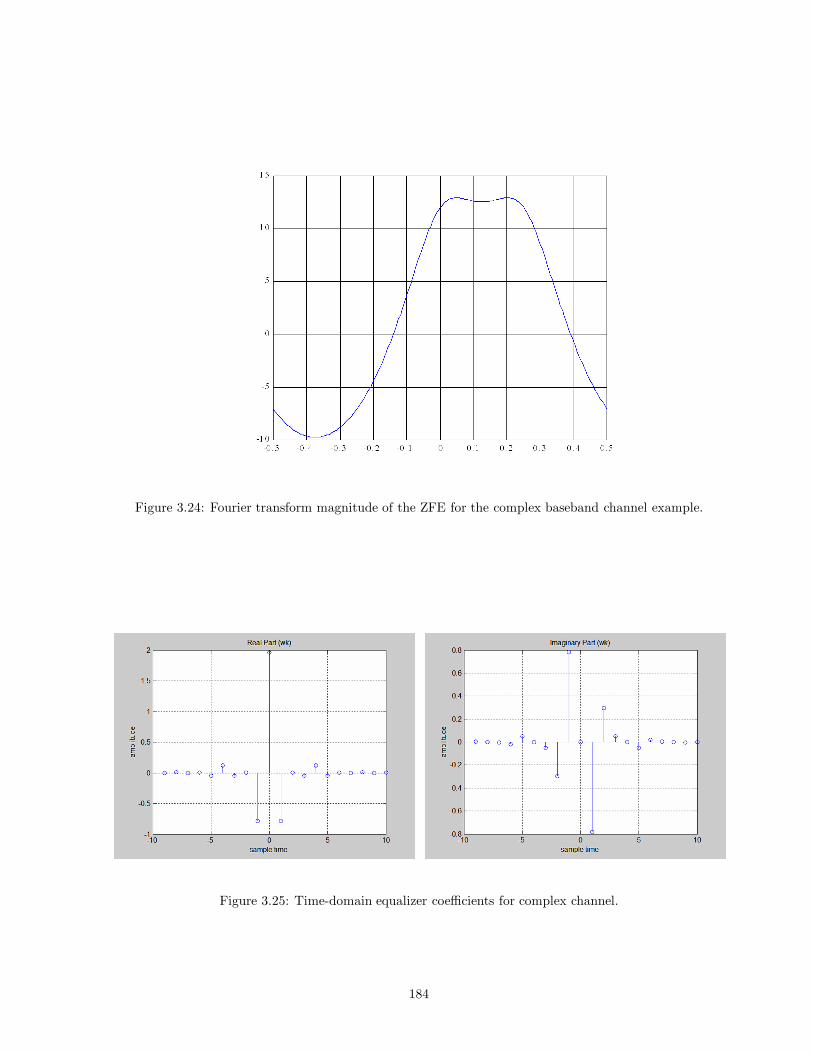
Figure 3.24: Fourier transform magnitude of the ZFE for the complex baseband channel example.
Figure 3.25: Time-domain equalizer coefficients for complex channel.
184

B =−4(−4)
(−2 − .5)(−2− 2)(−1.5)= .9412 + 1.5685 = 1.82936 1.030 . (3.137)
Finally
WZFE (D) =√
1.5625[
A(−.5)1 − .5D
+B(−.5)
(1 − .5D)+ terms
], (3.138)
and
w0 =√
1.5625 [(−.5)(−1.5686− .9412)− .5(.9412 + 1.5686)] (3.139)
=√
1.5625(1.57) = 1.96 (3.140)
The ZFE loss can be shown to be
γZFE = 10 · log10(w0 · ‖p‖) = 3.9 dB , (3.141)
which is better than the last channel because the frequency spectrum is not as near zeroin this complex example as it was earlier on the PAM example. Nevertheless, considerablybetter performance is also possible on this complex channel, but not with the ZFE.
To compute Pe for 4QAM, the designer calculates
Pe ≈ Q(√
SNRMFB − 3.9 dB)
. (3.142)
If SNRMFB = 10dB, then Pe ≈ 2.2× 10⁻². If SNRMFB = 17.4dB, then Pe ≈ 1.0× 10⁻⁶. IfSNRMFB = 23.4dB for 16QAM, then Pe ≈ 2.0× 10⁻⁵.
185

3.5 Minimum Mean-Square Error Linear Equalization
The Minimum Mean-Square Error Linear Equalizer (MMSE-LE) balances a reduction in ISIwith noise enhancement. The MMSE-LE always performs as well as, or better than, the ZFE and is ofthe same complexity of implementation. Nevertheless, it is slightly more complicated to describe andanalyze than is the ZFE. The MMSE-LE uses a linear time-invariant filter wk for R, but the choice offilter impulse response wk is different than the ZFE.
The MMSE-LE is a linear filter wk that acts on yk to form an output sequence zk that is the bestMMSE estimate of xk. That is, the filter wk minimizes the Mean Square Error (MSE):
Definition 3.5.1 (Mean Square Error (for the LE)) The LE error signal is given by
ek = xk − wk ∗ yk = xk − zk . (3.143)
The Minimum Mean Square Error (MMSE) for the linear equalizer is defined by
σ2MMSE−LE
∆= minwk
E[|xk − zk|2
]. (3.144)
The MSE criteria for filter design does not ignore noise enhancement because the optimization of thisfilter compromises between eliminating ISI and increasing noise power. Instead, the filter output is asclose as possible, in the Minimum MSE sense, to the data symbol xk.
3.5.1 Optimization of the Linear Equalizer
Using D-transforms,E(D) = X(D) − W (D)Y (D) (3.145)
By the orthogonality principle in Appendix A, at any time k, the error sample ek must be uncorrelatedwith any equalizer input signal ym. Succinctly,
E[E(D)Y ∗(D−∗)
]= 0 . (3.146)
Evaluating (3.146), using (3.145), yields
0 = Rxy(D) − W (D)Ryy(D) , (3.147)
where (N = 1 for PAM, N = 2 for Quadrature Modulation)9
Rxy(D) = E[X(D)Y ∗(D−∗)
]/N = ‖p‖Q(D)Ex
Ryy(D) = E[Y (D)Y ∗(D−∗)
]/N = ‖p‖2Q2(D)Ex +
N0
2Q(D) = Q(D)
(‖p‖2Q(D)Ex +
N0
2
).
Then the MMSE-LE becomes
W (D) =Rxy(D)Ryy(D)
=1
‖p‖ (Q(D) + 1/SNRMFB). (3.148)
The MMSE-LE differs from the ZFE only in the additive positive term in the denominator of (3.148).The transfer function for the equalizer W (e−ωT ) is also real and positive for all finite signal-to-noiseratios. This small positive term prevents the denominator from ever becoming zero, and thus makesthe MMSE-LE well defined even when the channel (or pulse response) is zero for some frequencies orfrequency bands. Also W (D) = W ∗(D−∗). Figure 3.26 repeats Figure 3.19 with addition of the MMSE-LE transfer characteristic. The MMSE-LE transfer function has magnitude Ex/σ2 at ω = π
T , while theZFE becomes infinite at this same frequency. This MMSE-LE leads to better performance, as the nextsubsection computes.
9The expression Rxx(D)∆= E
[X(D)X∗(D−∗)
]is used in a symbolic sense, since the terms of X(D)X∗(D−∗) are of
the form∑
kxkx∗
k−j, so that we are implying the additional operation limK→∞[1/(2K + 1)]∑
−K≤k≤Kon the sum in
such terms. This is permissable for stationary (and ergodic) discrete-time sequences.
186

Figure 3.26: Example of MMSE-LE versus ZFE.
3.5.2 Performance of the MMSE-LE
The MMSE is the time-0 coefficient of the error autocorrelation sequence
Ree(D) = E[E(D)E∗(D−∗)
]/N (3.149)
= Ex − W ∗(D−∗)Rxy(D) − W (D)R∗xy(D−∗) + W (D)Ryy(D)W ∗(D−∗) (3.150)
= Ex − W (D)Ryy(D)W ∗(D−∗) (3.151)
= Ex −Q(D)
(‖p‖2 · Q(D)Ex + N0
2
)
‖p‖2 (Q(D) + 1/SNRMFB)2(3.152)
= Ex − ExQ(D)(Q(D) + 1/SNRMFB)
(3.153)
=N02
‖p‖2 (Q(D) + 1/SNRMFB)(3.154)
The third equality follows from
W (D)Ryy(D)W ∗(D−∗) = W (D)Ryy(D)Ryy(D)−1R∗xy(D
−∗)
= W (D)R∗xy(D−∗) ,
and that(W (D)Ryy(D)W ∗(D−∗)
)∗ = W (D)Ryy(D)W ∗(D−∗). The MMSE then becomes
σ2MMSE−LE =
T
2π
∫ πT
− πT
Ree(e−ωT )dω =T
2π
∫ πT
− πT
N02 dω
‖p‖2 (Q(e−ωT ) + 1/SNRMFB). (3.155)
By recognizing that W (e−ωT ) is multiplied by the constant N02 /‖p‖ in (3.155), then
σ2MMSE−LE = w0
N02
‖p‖ . (3.156)
From comparison of (3.155) and (3.98), that
σ2MMSE−LE ≤ σ2
ZFE , (3.157)
with equality if and only if SNRMFB → ∞. Furthermore, since the ZFE is unbiased, and SNRMMSE−LE =SNRMMSE−LE,U +1 and SNRMMSE−LE,U are the maximum-SNR corresponding to unconstrained andunbiased linear equalizers, respectively,
SNRZFE ≤ SNRMMSE−LE,U =Ex
σ2MMSE−LE
− 1 ≤ SNRMFB . (3.158)
187
One confirms that the MMSE-LE is a biased receiver by writing the following expression for theequalizer output
Z(D) = W (D)Y (D) (3.159)
=1
‖p‖ (Q(D) + 1/SNRMFB)(Q(D)‖p‖X(D) + N (D)) (3.160)
= X(D) − 1/SNRMFB
Q(D) + 1/SNRMFBX(D) +
N (D)‖p‖ (Q(D) + 1/SNRMFB)
, (3.161)
for which the xk-dependent residual ISI term contains a component
signal-basis term = −1/SNRMFBw0 · ‖p‖ · xk (3.162)
= −1/SNRMFB ·σ2
MMSE−LE‖p‖2
N02
xk (3.163)
= −σ2
MMSE−LE
Ex· xk (3.164)
= −1
SNRMMSE−LE· xk . (3.165)
(3.166)
So zk =(1 − 1
SNRMMSE−LE
)xk − e′k where e′k is the error for unbiased detection and R. The optimum
unbiased receiver with decision regions scaled by 1 − 1
SNRMMSE−LE(see Section 3.2.1) has the signal
energy given by (1 − 1
SNRMMSE−LE
)2
Ex . (3.167)
A new error for the scaled decision regions is e′k = (1 − 1/SNRMMSE−LE) xk−zk = ek− 1
SNRMMSE−LExk,
which is also the old error with the xk dependent term removed. Since e′k and xk are then independent,then
σ2e = σ2
MMSE−LE = σ2e′ +
(1
SNRMMSE−LE
)2
Ex , (3.168)
leaving
σ2e′ = σ2
MMSE−LE−(
1SNRMMSE−LE
)2
Ex =SNR2
MMSE−LEσ2MMSE−LE − Ex
SNR2MMSE−LE
=Ex (SNRMMSE−LE − 1)
SNR2MMSE−LE
.
(3.169)The SNR for the unbiased MMSE-LE then becomes (taking the ratio of (3.167) to σ2
e′)
SNRMMSE−LE,U =
(SNRMMSE−LE−1)2
SNR2MMSE−LE
Ex
Ex (SNRMMSE−LE−1)
SNR2MMSE−LE
= SNRMMSE−LE − 1 , (3.170)
which corroborates the earlier result on the relation of the optimum biased and unbiased SNR’s for anyparticular receiver structure (at least for the LE structure). The unbiased SNR is
SNRMMSE−LE,U =Ex
σ2MMSE−LE
− 1 , (3.171)
which is the performance level that this text always uses because it corresponds to the best errorprobability for an SBS detector, as was discussed earlier in Section 3.1. Figure 3.27 illustrates theconcept with the effect of scaling on a 4QAM signal shown explicitly. Again, MMSE receivers (of whichthe MMSE-LE is one) reduce noise power at the expense of introducing a bias, the scaling up removes
188
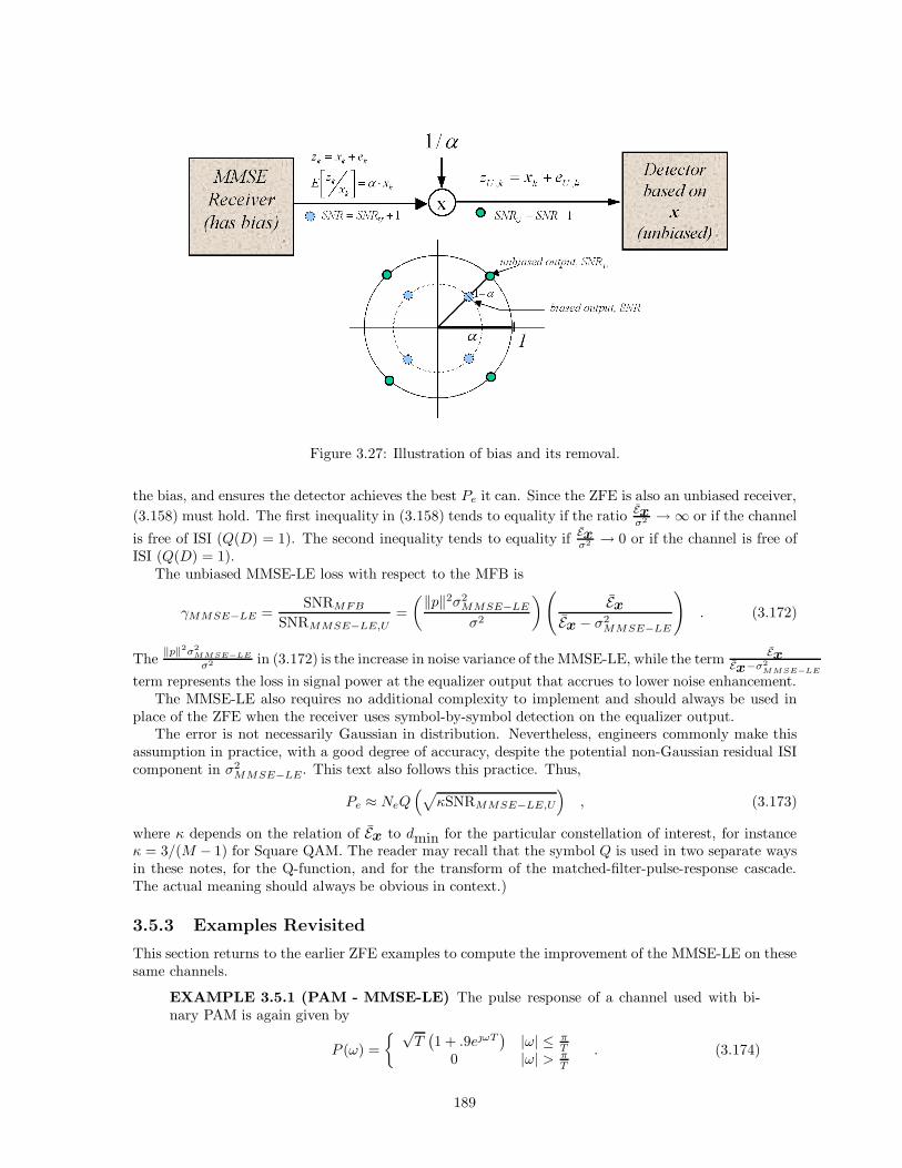
Figure 3.27: Illustration of bias and its removal.
the bias, and ensures the detector achieves the best Pe it can. Since the ZFE is also an unbiased receiver,(3.158) must hold. The first inequality in (3.158) tends to equality if the ratio Ex
σ2 → ∞ or if the channel
is free of ISI (Q(D) = 1). The second inequality tends to equality if Exσ2 → 0 or if the channel is free of
ISI (Q(D) = 1).The unbiased MMSE-LE loss with respect to the MFB is
γMMSE−LE =SNRMFB
SNRMMSE−LE,U=(‖p‖2σ2
MMSE−LE
σ2
)(Ex
Ex − σ2MMSE−LE
). (3.172)
The ‖p‖2σ2MMSE−LE
σ2 in (3.172) is the increase in noise variance of the MMSE-LE, while the term ExEx−σ2
MMSE−LE
term represents the loss in signal power at the equalizer output that accrues to lower noise enhancement.The MMSE-LE also requires no additional complexity to implement and should always be used in
place of the ZFE when the receiver uses symbol-by-symbol detection on the equalizer output.The error is not necessarily Gaussian in distribution. Nevertheless, engineers commonly make this
assumption in practice, with a good degree of accuracy, despite the potential non-Gaussian residual ISIcomponent in σ2
MMSE−LE. This text also follows this practice. Thus,
Pe ≈ NeQ(√
κSNRMMSE−LE,U
), (3.173)
where κ depends on the relation of Ex to dmin for the particular constellation of interest, for instanceκ = 3/(M − 1) for Square QAM. The reader may recall that the symbol Q is used in two separate waysin these notes, for the Q-function, and for the transform of the matched-filter-pulse-response cascade.The actual meaning should always be obvious in context.)
3.5.3 Examples Revisited
This section returns to the earlier ZFE examples to compute the improvement of the MMSE-LE on thesesame channels.
EXAMPLE 3.5.1 (PAM - MMSE-LE) The pulse response of a channel used with bi-nary PAM is again given by
P (ω) ={ √
T(1 + .9eωT
)|ω| ≤ π
T0 |ω| > π
T
. (3.174)
189

Figure 3.28: Comparison of equalizer frequency-domain responses for MMSE-LE and ZFE on basebandexample.
Let us suppose SNRMFB = 10dB (= Ex‖p‖2/N02 ) and that Ex = 1.
The equalizer is
W (D) =1
‖p‖ ·(
.91.81
D−1 + 1.1 + .91.81
D) . (3.175)
Figure 3.28 shows the frequency response of the equalizer for both the ZFE and MMSE-LE.Clearly the MMSE-LE has a lower magnitude in its response.
The σ2MMSE−LE is computed as
σ2MMSE−LE =
T
2π
∫ πT
− πT
N02
1.81 + 1.8 cos(ωT ) + 1.81/10dω (3.176)
=N0
21√
1.9912 − 1.82(3.177)
=N0
2(1.175) , (3.178)
which is considerably smaller than σ2ZFE. The SNR for the MMSE-LE is
SNRMMSE−LE,U =1 − 1.175(.181)
1.175(.181)= 3.7 (5.7dB) . (3.179)
The loss with respect to the MFB is 10dB - 5.7dB = 4.3dB. This is 5.5dB better than theZFE (9.8dB - 4.3dB = 5.5dB), but still not good for this channel.
Figure 3.29 compares the frequency-domain responses of the equalized channel. Figure 3.30compares the time-domain responses of the equalized channel. The MMSE-LE clearly doesnot have an ISI-free response, but mean-square error/distortion is minimized and the MMSE-LE has better performance than the ZFE.
The relatively small energy near the Nyquist Frequency in this example is the reason forthe poor performance of both linear equalizers (ZFE and MMSE-LE) in this example. To
190

Figure 3.29: Comparison of equalized frequency-domain responses for MMSE-LE and ZFE on basebandexample.
Figure 3.30: Comparison of equalized time-domain responses for MMSE-LE and ZFE on basebandexample.
191

Figure 3.31: Comparison of MMSE-LE and ZFE for complex channel example.
improve performance further, decision-assisted equalization is examined in Section 3.6 andin Chapter 5 (or codes combined with equalization, as discussed in Chapters 10 and 11).Another yet better method appears in Chapter 4.
The complex example also follows in a straightforward manner.
EXAMPLE 3.5.2 (QAM - MMSE-LE) Recall that the equivalent baseband pulse re-sponse samples were given by
pk =1√T
[−1
2,(1 +
4
), −
2
]. (3.180)
Again, SNRMFB = 10dB (= Ex‖p‖2/N02
), Ex = 1, and thus
σ2MMSE−LE = w0
N0
2‖p‖−1 . (3.181)
The equalizer is, noting that N02
= Ex‖p‖2
SNRMF B= 1.5625/10 = .15625,
W (D) =1
(Q(D) + 1/SNRMFB) ‖p‖ (3.182)
or
=√
1.5625−.25D−2 + .625(−1 + )D−1 + 1.5625(1 + .1) − .625(1 + )D1 + .25D2
. (3.183)
Figure 3.31 compares the MMSE-LE and ZFE equalizer responses for this same channel. TheMMSE-LE high response values are considerably more limited than the ZFE values. Theroots of Q(D) + 1/SNRMFB , or of the denominator in (3.183), are
D = 2.2176 −1.632 = −.1356− 2.213 (3.184)D = 2.2176 .0612 = 2.213 + .1356 (3.185)D = .4516 −1.632 = −.0276− .4502 (3.186)D = .4516 .0612 = .4502 + .0276 , (3.187)
192

and (3.183) becomes
W (D) =
[√1.5625D2/(.25)
]
(D − 2.226 −1.632)(D − 2.226 .0612)(D − .4516 −1.632)(D − .4516 .0612)(3.188)
orW (D) =
A
D − 2.226 −1.632 +B
D − 2.226 .0612 + ... , (3.189)
where the second expression (3.189) has ignored any terms in the partial fraction expansionthat will not contribute to w0. Then,
A =√
1.5625(−4)(2.226 −1.632)2
(2.226 −1.632 − 2.226 .0612)(2.226 −1.632 − .4516 −1.632)(2.226 −1.632 − .4516 .0612)
=√
1.5625(−.805 + 1.20) = 1.0079 + 1.5025 (3.190)
B =√
1.5625(−4)(2.226 .0612)2
(2.226 .0612 − 2.226 −1.632)(2.226 .0612 − .4516 −1.632)(2.226 .0612 − .4516 .0612)
=√
1.5625(1.20− .805) = −1.5025− 1.0079 . (3.191)
Then, from (3.189),
w0 = A(−.4516 1.632) + B(−.4516 −.0612) =√
1.5625(1.125) . (3.192)
Thenσ2
MMSE−LE = 1.125N0
2= 1.125(.15625) = .1758 , (3.193)
SNRMMSE−LE,U =[1 − 1.125(.15625)]
1.125(.15625)= 4.69 ( 6.7 dB ) , (3.194)
which is 3.3 dB below the matched filter bound SNR of 10dB, or equivalently,
γMMSE−LE = 10 log10(10/4.69) = 10 log10(2.13) = 3.3 dB , (3.195)
but .6 dB better than the ZFE. It is also possible to do considerably better on this channel,but structures not yet introduced will be required. Nevertheless, the MMSE-LE is one of themost commonly used equalization structures in practice.
Figure 3.31 compares the equalized channel responses for both the MMSE-LE and ZFE.While the MMSE-LE performs better, there is a significant deviation from the ideal flatresponse. This deviation is good and gains .6 dB improvement. Also, because of biasing,the MMSE-LE output is everywhere slightly lower than the ZFE output (which is unbiased).This bias can be removed by scaling by 5.69/4.69.
3.5.4 Fractionally Spaced Equalization
To this point in the study of the discrete time equalizer, a matched filter ϕ∗p(−t) precedes the sampler,
as was shown in Figure 3.7. While this may be simple from an analytical viewpoint, there are severalpractical problems with the use of the matched filter. First, ϕ∗
p(−t) is a continuous time filter andmay be much more difficult to design accurately than an equivalent digital filter. Secondly, the precisesampling frequency and especially its phase, must be known so that the signal can be sampled when it isat maximum strength. Third, the channel pulse response may not be accurately known at the receiver,and an adaptive equalizer (see Chapter 7), is instead used. It may be difficult to design an adaptive,analog, matched filter.
For these reasons, sophisticated data transmission systems often replace the matched-filter/sampler/equalizersystem of Figure 3.7 with the Fractionally Spaced Equalizer (FSE) of Figure 3.32. Basically, the samplerand the matched filter have been interchanged with respect to Figure 3.7. Also the sampling rate hasbeen increased by some rational number l (l > 1). The new sampling rate is chosen sufficiently high so
193
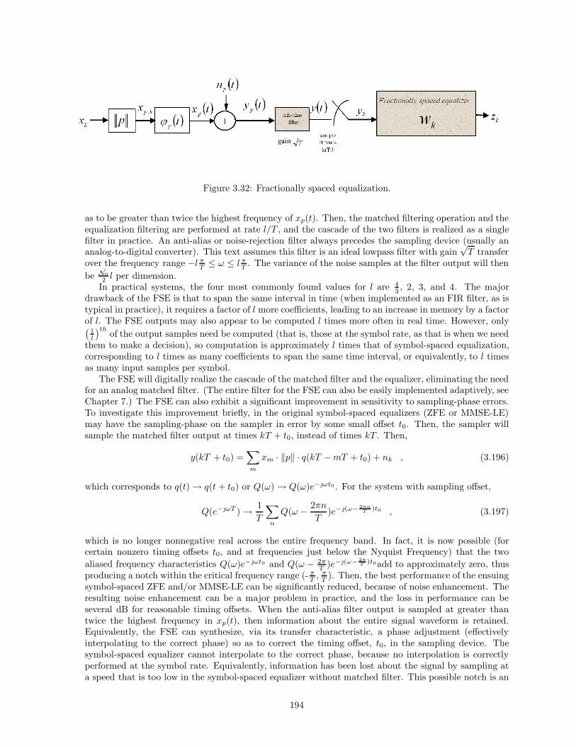
Figure 3.32: Fractionally spaced equalization.
as to be greater than twice the highest frequency of xp(t). Then, the matched filtering operation and theequalization filtering are performed at rate l/T , and the cascade of the two filters is realized as a singlefilter in practice. An anti-alias or noise-rejection filter always precedes the sampling device (usually ananalog-to-digital converter). This text assumes this filter is an ideal lowpass filter with gain
√T transfer
over the frequency range −l πT≤ ω ≤ l π
T. The variance of the noise samples at the filter output will then
be N02 l per dimension.In practical systems, the four most commonly found values for l are 4
3, 2, 3, and 4. The major
drawback of the FSE is that to span the same interval in time (when implemented as an FIR filter, as istypical in practice), it requires a factor of l more coefficients, leading to an increase in memory by a factorof l. The FSE outputs may also appear to be computed l times more often in real time. However, only(
1l
)th of the output samples need be computed (that is, those at the symbol rate, as that is when we needthem to make a decision), so computation is approximately l times that of symbol-spaced equalization,corresponding to l times as many coefficients to span the same time interval, or equivalently, to l timesas many input samples per symbol.
The FSE will digitally realize the cascade of the matched filter and the equalizer, eliminating the needfor an analog matched filter. (The entire filter for the FSE can also be easily implemented adaptively, seeChapter 7.) The FSE can also exhibit a significant improvement in sensitivity to sampling-phase errors.To investigate this improvement briefly, in the original symbol-spaced equalizers (ZFE or MMSE-LE)may have the sampling-phase on the sampler in error by some small offset t0. Then, the sampler willsample the matched filter output at times kT + t0, instead of times kT . Then,
y(kT + t0) =∑
m
xm · ‖p‖ · q(kT − mT + t0) + nk , (3.196)
which corresponds to q(t) → q(t + t0) or Q(ω) → Q(ω)e−ωt0 . For the system with sampling offset,
Q(e−ωT ) → 1T
∑
n
Q(ω − 2πn
T)e−(ω− 2πn
T )t0 , (3.197)
which is no longer nonnegative real across the entire frequency band. In fact, it is now possible (forcertain nonzero timing offsets t0, and at frequencies just below the Nyquist Frequency) that the twoaliased frequency characteristics Q(ω)e−ωt0 and Q(ω − 2π
T)e−(ω− 2π
T )t0add to approximately zero, thusproducing a notch within the critical frequency range (- π
T, π
T). Then, the best performance of the ensuing
symbol-spaced ZFE and/or MMSE-LE can be significantly reduced, because of noise enhancement. Theresulting noise enhancement can be a major problem in practice, and the loss in performance can beseveral dB for reasonable timing offsets. When the anti-alias filter output is sampled at greater thantwice the highest frequency in xp(t), then information about the entire signal waveform is retained.Equivalently, the FSE can synthesize, via its transfer characteristic, a phase adjustment (effectivelyinterpolating to the correct phase) so as to correct the timing offset, t0, in the sampling device. Thesymbol-spaced equalizer cannot interpolate to the correct phase, because no interpolation is correctlyperformed at the symbol rate. Equivalently, information has been lost about the signal by sampling ata speed that is too low in the symbol-spaced equalizer without matched filter. This possible notch is an
194

example of information loss at some frequency; this loss cannot be recovered in a symbol-spaced equalizerwithout a matched filter. In effect, the FSE equalizes before it aliases (aliasing does occur at the outputof the equalizer where it decimates by l for symbol-by-symbol detection), whereas the symbol-spacedequalizer aliases before it equalizes; the former alternative is often the one of choice in practical systemimplementation, if the extra memory and computation can be accommodated. Effectively, with an FSE,the sampling device need only be locked to the symbol rate, but can otherwise provide any samplingphase. The phase is tacitly corrected to the optimum phase inside the linear filter implementing theFSE.
The sensitivity to sampling phase is channel dependent: In particular, there is usually significantchannel energy near the Nyquist Frequency in applications that exhibit a significant improvement ofthe FSE with respect to the symbol-spaced equalizer. In channels with little energy near the NyquistFrequency, the FSE is avoided, because it provides little performance gain, and is significantly morecomplex to implement (more parameters and higher sampling rate).
Infinite-Length FSE Settings To derive the settings for the FSE, this section assumes that l, theoversampling factor, is an integer. The sampled output of the anti-alias filter can be decomposed into lsampled-at-rate-1/T interleaved sequences with D-transforms Y0(D), Y2(D), ..., Yl−1(D), where Yl(D)corresponds to the sample sequence y[kT − iT/l]. Then,
Yi(D) = Pi(D) · X(D) + Ni(D) (3.198)
where Pi(D) is the transform of the symbol-rate-spaced-ith-phase-of-p(t) sequence p[kT − (i − 1)T/l],and similarly Ni(D) is the transform of a symbol-rate sampled white noise sequence with autocorrelationfunction Rnn(D) = l · N0
2per dimension, and these noise sequences are also independent of one another.
A column vector transform is
Y (D) =
Y0(D)...
Yl−1(D)
= P (D)X(D) + N (D) . (3.199)
Also
P (D) ∆=
P0(D)...
Pl−1(D)
and N (D) =
N0(D)...
Nl−1(D)
. (3.200)
By considering the FSE output at sampling rate 1/T , the interleaved coefficients of the FSE can also bewritten in a row vector W (D) = [W1(D) , ..., Wl(D)]. Thus the FSE output is
Z(D) = W (D)Y (D) . (3.201)
Again, the orthogonality condition says that E(D) = X(D) − Z(D) should be orthogonal to Y (D),which can be written in vector form as
E[E(D)Y ∗(D−∗)
]= RxY (D) − W (D)RY Y (D) = 0 , (3.202)
where
RxY (D) ∆= E
[X(D)Y ∗(D−∗)
]= ExP ∗(D−∗) (3.203)
RY Y (D) ∆= E[Y (D)Y ∗(D−∗)
]= ExP (D)P ∗(D−∗) + l · N0
2I . (3.204)
MMSE-FSE filter setting is then
W (D) = RxY (D)R−1
Y Y(D) = P ∗(D−∗)
[P (D)P ∗(D−∗) + l/SNR
]−1. (3.205)
The corresponding error sequence has autocorrelation function
Ree(D) = Ex − RxY (D)R−1
Y Y(D)RY x
(D) =l · N0
2
P ∗(D−∗)P (D) + l/SNR. (3.206)
195

Figure 3.33: Passband equalization, direct synthesis of analytic-equivalent equalizer.
The MMSE is then computed as
MMSEMMSE−FSE =T
2π
∫ πT
− πT
l · N02
dω
‖P (e−ωT )‖2 + l/SNR= MMSEMMSE−LE , (3.207)
where ‖P (e−ωT )‖2 =∑l
i=1 |Pi(e−ωT )|2. The SNR’s, biased and unbiased, are also then exactly thesame as given for the MMSE-LE, as long as the sampling rate exceeds twice the highest frequency ofP (f).
The reader is cautioned against letting N02 → 0 to get the ZF-FSE. This is because the matrix
RY Y (D) will often be singular when this occurs. To avoid problems with singularity, an appropriatepseudoinverse, which zeros the FSE characteristic when P (ω) = 0 is recommended.
Passband Equalization
This chapter so far assumed for the complex baseband equalizer that the passband signal has been de-modulated according to the methods described in Chapter 2 before filtering and sampling. An alternativemethod, sometimes used in practice when ωc is not too high (or intermediate-frequency up/down con-version is used), is to commute the demodulation and filtering functions. Sometimes this type of systemis also called “direct conversion,” meaning that no carrier demodulation occurs prior to sampling. Thiscommuting can be done with either symbol-spaced or fractionally spaced equalizers. The main reasonfor the interchange of filtering and demodulation is the recovery of the carrier frequency in practice.Postponing the carrier demodulation to the equalizer output can lead to significant improvement in thetolerance of the system to any error in estimating the carrier frequency, as Chapter 6 investigates. In thepresent (perfect carrier phase lock) development, passband equalization and baseband equalization areexactly equivalent and the settings for the passband equalizer are identical to those of the correspondingbaseband equalizer, other than a translation in frequency by ωc radians/sec.
Passband equalization is best suited to CAP implementations (See Section 4 of Chapter 2) where thecomplex channel is the analytic equivalent. The complex equalizer then acts on the analytic equivalentchannel and signals to eliminate ISI in a MMSE sense. When used with CAP, the final rotation shownin Figure 3.33 is not necessary – such a rotation is only necessary with a QAM transmit signal.
The passband equalizer is illustrated in Figure 3.33. The phase splitting is the forming of the analyticequivalent with the use of the Hilbert Transform, as discussed in Chapter 2. The matched filtering andequalization are then performed on the passband signal with digital demodulation to baseband deferredto the filter output. The filter wk can be a ZFE, a MMSE-LE, or any other desired setting (see Chapter4 and Sections 3.5 and 3.6). In practice, the equalizer can again be realized as a fractionally spacedequalizer by interchanging the positions of the matched filter and sampler, increasing the sampling rate,and absorbing the matched filtering operation into the filter wk, which would then be identical to the(modulated) baseband-equivalent FSE with output sample rate decimated appropriately to produceoutputs only at the symbol sampling instants.
Often in practice, the cross-coupled nature of the complex equalizer W (D) is avoided by sampling theFSE at a rate that exceeds twice the highest frequency of the passband signal y(t) prior to demodulation.(If intermediate frequency (IF) demodulation is used, then twice the highest frequency after the IF.) In
196

this case the phase splitter (contains Hilbert transform in parallel with a unit gain) is also absorbed intothe equalizer, and the same sampled sequence is applied independently to two equalizers, one of whichestimates the real part, and one the imaginary part, of the analytic representation of the data sequencexkeωckT . The two filters can sometimes (depending on the sampling rate) be more cost effective toimplement than the single complex filter, especially when one considers that the Hilbert transform isincorporated into the equalizer. This approach is often taken with adaptive implementations of theFSE, as the Hilbert transform is then implemented more exactly adaptively than is possible with fixeddesign.10 This is often called Nyquist Inband Equalization. A particularly common variant of thistype of equalization is to sample at rate 2/T both of the outputs of a continuous-time phase splitter,one stream of samples staggered by T/4 with respect to the other. The corresponding T/2 complexequalizer can then be implemented adaptively with four independent adaptive equalizers (rather thanthe two filters, real and imaginary part, that nominally characterize complex convolution). The adaptivefilters will then correct for any imperfections in the phase-splitting process, whereas the two filters withfixed conjugate symmetry could not.
10However, this structure also slows convergence of many adaptive implementations.
197
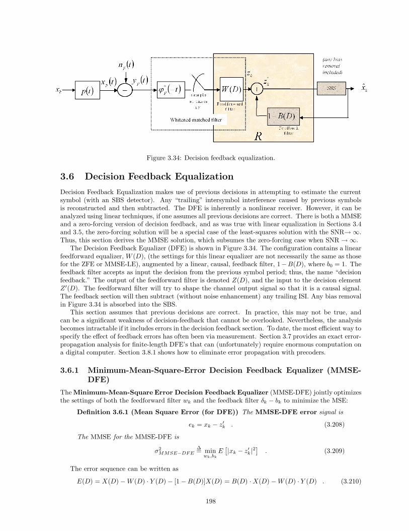
Figure 3.34: Decision feedback equalization.
3.6 Decision Feedback Equalization
Decision Feedback Equalization makes use of previous decisions in attempting to estimate the currentsymbol (with an SBS detector). Any “trailing” intersymbol interference caused by previous symbolsis reconstructed and then subtracted. The DFE is inherently a nonlinear receiver. However, it can beanalyzed using linear techniques, if one assumes all previous decisions are correct. There is both a MMSEand a zero-forcing version of decision feedback, and as was true with linear equalization in Sections 3.4and 3.5, the zero-forcing solution will be a special case of the least-squares solution with the SNR→ ∞.Thus, this section derives the MMSE solution, which subsumes the zero-forcing case when SNR → ∞.
The Decision Feedback Equalizer (DFE) is shown in Figure 3.34. The configuration contains a linearfeedforward equalizer, W (D), (the settings for this linear equalizer are not necessarily the same as thosefor the ZFE or MMSE-LE), augmented by a linear, causal, feedback filter, 1−B(D), where b0 = 1. Thefeedback filter accepts as input the decision from the previous symbol period; thus, the name “decisionfeedback.” The output of the feedforward filter is denoted Z(D), and the input to the decision elementZ′(D). The feedforward filter will try to shape the channel output signal so that it is a causal signal.The feedback section will then subtract (without noise enhancement) any trailing ISI. Any bias removalin Figure 3.34 is absorbed into the SBS.
This section assumes that previous decisions are correct. In practice, this may not be true, andcan be a significant weakness of decision-feedback that cannot be overlooked. Nevertheless, the analysisbecomes intractable if it includes errors in the decision feedback section. To date, the most efficient way tospecify the effect of feedback errors has often been via measurement. Section 3.7 provides an exact error-propagation analysis for finite-length DFE’s that can (unfortunately) require enormous computation ona digital computer. Section 3.8.1 shows how to eliminate error propagation with precoders.
3.6.1 Minimum-Mean-Square-Error Decision Feedback Equalizer (MMSE-DFE)
The Minimum-Mean-Square Error Decision Feedback Equalizer (MMSE-DFE) jointly optimizesthe settings of both the feedforward filter wk and the feedback filter δk − bk to minimize the MSE:
Definition 3.6.1 (Mean Square Error (for DFE)) The MMSE-DFE error signal is
ek = xk − z′k . (3.208)
The MMSE for the MMSE-DFE is
σ2MMSE−DFE
∆= minwk,bk
E[|xk − z′k|2
]. (3.209)
The error sequence can be written as
E(D) = X(D) − W (D) · Y (D) − [1 − B(D)]X(D) = B(D) · X(D) − W (D) · Y (D) . (3.210)
198

For any fixed B(D), E [E(D)Y ∗(D−∗)] = 0 to minimize MSE, which leads us to the relation
B(D) · Rxy(D) − W (D) · Ryy(D) = 0 . (3.211)
Thus,
W (D) =B(D)
‖p‖(Q(D) + 1
SNRMF B
) = B(D) · WMMSE-LE(D) , (3.212)
for any B(D) with b0 = 1. (Also, W (D) = WMMSE-LE(D) · B(D), a consequence of the linearity ofthe MMSE estimate, so that E(D) = B(D) · EMMSE-LE(D))
The autocorrelation function for the error sequence with arbitrary monic B(D) is
Ree(D) = B(D)ExB∗(D−∗) − 2<{B(D)Rxy(D)W ∗(D−∗)
}+ W (D)Ryy(D)W ∗(D−∗)(3.213)
= B(D)ExB∗(D−∗) − W (D)Ryy(D)W ∗(D−∗) (3.214)
= B(D)ExB∗(D−∗) − B(D)Rxy(D)
‖p‖(Q(D) + 1
SNRMFB
)B∗(D−∗) (3.215)
= B(D)RMMSE−LE(D)B∗(D−∗) (3.216)
where RMMSE−LE(D) =N02
‖p‖2 1/(Q(D) + 1/SNRMFB) is the autocorrelation function for the errorsequence of a MMSE linear equalizer. The solution for B(D) is then the forward prediction filterassociated with this error sequence as discussed in the Appendix. The linear prediction approach isdeveloped more in what is called the “linear prediction DFE,” in an exercise where the MMSE-DFE isthe concatenation of a MMSE-LE and a linear-predictor that whitens the error sequence.
In more detail on B(D), the (scaled) inverse autocorrelation has spectral factorization:
Q(D) +1
SNRMFB= γ0 ·G(D) · G∗(D−∗), (3.217)
where γ0 is a positive real number and G(D) is a canonical filter response. A filter response G(D) iscalled canonical if it is causal (gk = 0 for k < 0), monic (g0 = 1), and minimum-phase (all its polesare outside the unit circle, and all its zeroes are on or outside the unit circle). If G(D) is canonical,then G∗(D−∗) is anti-canonical i.e., anti-causal, monic, and “maximum-phase” (all poles inside theunit circle, and all zeros in or on the unit circle). Using this factorization,
Ree(D) =B(D) · B∗(D−∗)
Q(D) + 1/SNRMFB·
N02
‖p‖2(3.218)
=B(D)G(D)
· B∗(D−∗)G∗(D−∗)
·N02
γ0‖p‖2(3.219)
ree,0 ≥N02
γ0‖p‖2, (3.220)
with equality if and only if B(D) = G(D). Thus, the MMSE will then be σ2MMSE−DFE =
N02
γ0‖p‖2 . Thefeedforward filter then becomes
W (D) =G(D)
‖p‖ · γ0 · G(D) · G∗(D−∗)=
1‖p‖ · γ0 · G∗(D−∗)
. (3.221)
The last step in (3.220) follows from the observations that
ree,0 = ‖B
G‖2
N02
γ0 · ‖p‖2, (3.222)
the fractional polynomial inside the squared norm is necessary monic and causal, and therefore thesquared norm has a minimum value of 1. B(D) and W (D) specify the MMSE-DFE:
199

Lemma 3.6.1 (MMSE-DFE) The MMSE-DFE has feedforward section
W (D) =1
‖p‖ · γ0 · G∗(D−∗)(3.223)
(realized with delay, as it is strictly noncausal) and feedback section
B(D) = G(D) (3.224)
where G(D) is the unique canonical factor of the following equation:
Q(D) +1
SNRMFB= γ0 · G(D) ·G∗(D−∗) . (3.225)
This text also calls the joint matched-filter/sampler/W (D) combination in the forward path ofthe DFE the “Mean-Square Whitened Matched Filter (MS-WMF)”. These settingsfor the MMSE-DFE minimize the MSE as was shown above.
3.6.2 Performance Analysis of the MMSE-DFE
Again, the autocorrelation function for the error sequence is
Ree(D) =N02
γ0 · ‖p‖2. (3.226)
This last result states that the error sequence for the MMSE-DFE is “white” when minimized (since
Ree(D) is a constant) and has MMSE or average energy (per real dimension)N02
‖p‖2 γ−10 . Also,
T
2π
∫ πT
− πT
ln(
Q(e−ωT ) +1
SNRMFB
)dω = ln(γ0) +
T
2π
∫ πT
− πT
ln(G(e−ωT )G∗(e−ωT )
)dω(3.227)
= ln(γ0) . (3.228)
This last result leads to a famous expression for σ2MMSE−DFE , which was first derived by Salz in 1973,
σ2MMSE−DFE =
N02
‖p‖2· e− T
2π
∫ πT− π
Tln(Q(e−ωT ) + 1
SNRMFB
)dω
. (3.229)
The SNR for the MMSE-DFE can now be easily computed as
SNRMMSE−DFE =Ex
σ2MMSE−DFE
= γ0 · SNRMFB (3.230)
= SNRMFBe
T2π
∫ πT− π
Tln(Q(e−ωT ) + 1
SNRMFB
)dω
. (3.231)
From the k = 0 term in the defining spectral factorization, γ0 can also be written
γ0 =1 + 1/SNRMFB
‖g‖2=
1 + 1/SNRMFB
1 +∑∞
i=1 |gi|2. (3.232)
From this expression, if G(D) = 1 (no ISI), then SNRMMSE−DFE = SNRMFB + 1, so that the SNRwould be higher than the matched filter bound. The reason for this apparent anomaly is the artificialsignal power introduced by biased decision regions. This bias is noted by writing
Z′(D) = X(D) − E(D) (3.233)
= X(D) − G(D) · X(D) +1
‖p‖ · γ0 · G∗(D−∗)Y (D) (3.234)
= X(D) − G(D)X(D) +Q(D)
γ0G∗(D−∗)X(D) + N (D)
1‖p‖γ0G∗(D−∗)
(3.235)
= X(D) − 1/SNRMFB
γ0 · G∗(D−∗)X(D) + N (D)
1‖p‖ · γ0 ·G∗(D−∗)
. (3.236)
200

The current sample, xk, corresponds to the time zero sample of 1 − 1/SNRMFB
γ0·G∗(D−∗) , and is equal to (1 −1
SNRMMSE−DFE)xk. Thus z′k contains a signal component of xk that is reduced in magnitude. Thus,
again using the result from Section 3.2.1, the SNR corresponding to the lowest probability of errorcorresponds to the same MMSE-DFE receiver with output scaled to remove the bias. This leads to themore informative SNR
SNRMMSE−DFE,U = SNRMMSE−DFE − 1 = γ0 · SNRMFB − 1 . (3.237)
If G(D) = 1, then SNRMMSE−DFE,U = SNRMFB . Also,
γMMSE−DFE =SNRMFB
SNRMMSE−DFE,U=
SNRMFB
γ0 · SNRMFB − 1=
1γ0 − 1/SNRMFB
. (3.238)
Rather than scale the decision input, the receiver can scale (up) the feedforward output by 11− 1
SNRMMSE−DF E
.
This will remove the bias, but also increase MSE by the square of the same factor. The SNR will thenbe SNRMMSE−DFE,U . This result is verified by writing the MS-WMF output
Z(D) = [X(D) · ‖p‖ · Q(D) + N (D)]1
‖p‖ · γ0 · G∗(D−∗)(3.239)
where N (D), again, has autocorrelation Rnn(D) = N02 Q(D). Z(D) expands to
Z(D) = [X(D) · ‖p‖ · Q(D) + N (D)]1
‖p‖ · γ0 · G∗(D−∗)(3.240)
= X(D)γ0 · G(D) ·G∗(D−∗) − 1/SNRMFB
γ0 · G∗(D−∗)+ N (D)
1‖p‖ · γ0 · G∗(D−∗)
(3.241)
= X(D) · G(D) − X(D)SNRMFB · γ0 · G∗(D−∗)
+ N ′(D) (3.242)
= X(D)[G(D) − 1
SNRMMSE−DFE
]+
1SNRMMSE−DFE
[1 − 1
G∗(D−∗)
]X(D) + N ′(D)(3.243)
= X(D)[G(D) − 1
SNRMMSE−DFE
]+ E′(D) , (3.244)
where N ′(D) is the filtered noise at the MS-WMF output, and has autocorrelation function
Rn′n′(D) =N02 Q(D)
‖p‖2 · γ20 · G(D) ·G∗(D−∗)
=Ex
SNRMMSE−DFE
[1 − 1/SNRMFB
Q(D) + 1/SNRMFB
], (3.245)
ande′k = −ek +
1SNRMMSE−DFE
xk . (3.246)
The error e′k is not a white sequence in general. Since xk and e′k are uncorrelated, σ2e = σ2
MMSE−DFE =
σ2e′ + Ex
SNR2MMSE−DF E
. If one defines an “unbiased” monic, causal polynomial
GU(D) =SNRMMSE−DFE
SNRMMSE−DFE,U
[G(D) − 1
SNRMMSE−DFE
], (3.247)
then the MMSE-DFE output is
Z(D) =SNRMMSE−DFE,U
SNRMMSE−DFEX(D)GU (D) + E′(D) . (3.248)
ZU (D) removes the scaling
ZU (D) = Z(D)SNRMMSE−DFE
SNRMMSE−DFE,U= X(D)GU (D) + EU (D) , (3.249)
201

Figure 3.35: Decision feedback equalization with unbiased feedback filter.
where EU(D) = SNRMMSE−DF E
SNRMMSE−DF E,UE′(D) and has power
σ2eU
=
(σ2
MMSE−DFE − ExSNR2
MMSE−DFE
)(SNRMMSE−DFE
SNRMMSE−DFE,U
)2
(3.250)
=SNR2
MMSE−DFEσ2MMSE−DFE − Ex
SNR2MMSE−DFE
SNR2MMSE−DFE
SNR2MMSE−DFE,U
(3.251)
=Ex[(SNRMMSE−DFE/Ex)SNRMMSE−DFEσ2
MMSE−DFE − 1]SNR2
MMSE−DFE,U
(3.252)
=Ex[SNRMMSE−DFE − 1]
SNR2MMSE−DFE,U
(3.253)
=Ex
SNRMMSE−DFE,U. (3.254)
SNR for this scaled and unbiased MMSE-DFE is thus verified to be ExEx/SNRMMSE−DFE,U
= SNRMMSE−DFE,U .
The feedback section of this new unbiased MMSE-DFE becomes the polynomial 1−GU(D), if the scalingis performed before the summing junction, but is 1 − G(D) if scaling is performed after the summingjunction. The alternative unbiased MMSE-DFE is shown in Figure 3.35.
All the results on fractional spacing for the LE still apply to the feedforward section of the DFE– thus this text does not reconsider them for the DFE, other than to state that the characteristic ofthe feedforward section is different than the LE characteristic in all but trivial channels. Again, therealization of any characteristic can be done with a matched filter and symbol-spaced sampling or withan anti-alias filter and fractionally spaced sampling, as in Section 3.5.4.
3.6.3 Zero-Forcing DFE
The ZF-DFE feedforward and feedback filters are found by setting SNRMFB → ∞ in the expressionsfor the MMSE-DFE. The spectral factorization (assuming ln(Q(eωT ) is integrable over (− π
T , πT ), see
Appendix A)Q(D) = η0 · Pc(D) · P ∗
c (D−∗) (3.255)
then determines the ZF-DFE filters asB(D) = Pc(D) , (3.256)
W (D) =1
η0 · ‖p‖ · P ∗c (D−∗)
. (3.257)
Pc is sometimes called a canonical pulse response for the channel. Since q0 = 1 = η0 · ‖Pc‖2, then
η0 =1
1 +∑∞
i=1 |pc,i|2. (3.258)
202
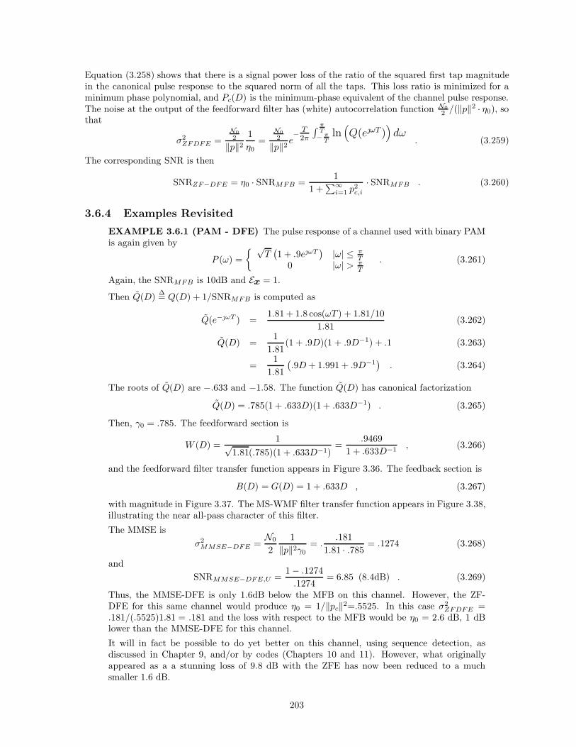
Equation (3.258) shows that there is a signal power loss of the ratio of the squared first tap magnitudein the canonical pulse response to the squared norm of all the taps. This loss ratio is minimized for aminimum phase polynomial, and Pc(D) is the minimum-phase equivalent of the channel pulse response.The noise at the output of the feedforward filter has (white) autocorrelation function N0
2 /(‖p‖2 · η0), sothat
σ2ZFDFE =
N02
‖p‖2
1η0
=N02
‖p‖2e−
T2π
∫ πT− π
Tln(Q(eωT )
)dω
. (3.259)
The corresponding SNR is then
SNRZF−DFE = η0 · SNRMFB =1
1 +∑∞
i=1 p2c,i
· SNRMFB . (3.260)
3.6.4 Examples Revisited
EXAMPLE 3.6.1 (PAM - DFE) The pulse response of a channel used with binary PAMis again given by
P (ω) ={ √
T(1 + .9eωT
)|ω| ≤ π
T0 |ω| > π
T
. (3.261)
Again, the SNRMFB is 10dB and Ex = 1.
Then Q(D) ∆= Q(D) + 1/SNRMFB is computed as
Q(e−ωT ) =1.81 + 1.8 cos(ωT ) + 1.81/10
1.81(3.262)
Q(D) =1
1.81(1 + .9D)(1 + .9D−1) + .1 (3.263)
=1
1.81(.9D + 1.991 + .9D−1
). (3.264)
The roots of Q(D) are −.633 and −1.58. The function Q(D) has canonical factorization
Q(D) = .785(1 + .633D)(1 + .633D−1) . (3.265)
Then, γ0 = .785. The feedforward section is
W (D) =1√
1.81(.785)(1 + .633D−1)=
.94691 + .633D−1
, (3.266)
and the feedforward filter transfer function appears in Figure 3.36. The feedback section is
B(D) = G(D) = 1 + .633D , (3.267)
with magnitude in Figure 3.37. The MS-WMF filter transfer function appears in Figure 3.38,illustrating the near all-pass character of this filter.
The MMSE isσ2
MMSE−DFE =N0
21
‖p‖2γ0= .
.1811.81 · .785
= .1274 (3.268)
andSNRMMSE−DFE,U =
1 − .1274.1274
= 6.85 (8.4dB) . (3.269)
Thus, the MMSE-DFE is only 1.6dB below the MFB on this channel. However, the ZF-DFE for this same channel would produce η0 = 1/‖pc‖2=.5525. In this case σ2
ZFDFE =.181/(.5525)1.81 = .181 and the loss with respect to the MFB would be η0 = 2.6 dB, 1 dBlower than the MMSE-DFE for this channel.
It will in fact be possible to do yet better on this channel, using sequence detection, asdiscussed in Chapter 9, and/or by codes (Chapters 10 and 11). However, what originallyappeared as a a stunning loss of 9.8 dB with the ZFE has now been reduced to a muchsmaller 1.6 dB.
203

Figure 3.36: Feedforward filter transfer function for real-channel example.
Figure 3.37: Feedback filter transfer function for real-channel example.
204

Figure 3.38: MS-WMF transfer function for real-channel example.
The QAM example is also revisited here:
EXAMPLE 3.6.2 (QAM - DFE) Recall that the equivalent baseband pulse responsesamples were given by
pk =1√T
[−1
2
(1 +
4
)−
2
]. (3.270)
The SNRMFB is again 10 dB. Then,
Q =−.25D−2 + .625(−1 + )D−1 + 1.5625(1 + .1) − .625(1 + )D + .25D2
1.5625. (3.271)
or
Q = (1 − .4516 1.632D)(1 − .4516 −.0612D)(1 − .4516 −1.632D−1)(1 − .4516 .0612D−1) ·
· −
1.5625 · 4 · (.4516 −1.632)(.4516 .0612)(3.272)
from which one extracts γ0 = .7866 and G(D) = 1−.4226(1+)D+.2034D2. The feedforwardand feedback sections can be computed in a straightforward manner, as
B(D) = G(D) = 1 − .4226(1 + )D + .2034D2 (3.273)
andW (D) =
1.0171 − .4226(1− )D−1 − .2034D−2
. (3.274)
The MSE isσ2
MMSE−DFE = (.15625)1
.7866(1.5625)= .1271 . (3.275)
and the corresponding SNR is
SNRMMSE−DFE,U =1
.1271− 1 = 8.4dB . (3.276)
205

The loss is (also coincidentally) 1.6 dB with respect to the MFB and is 1.7 dB better thanthe MMSE-LE on this channel.
For the ZF-DFE,
Q(D) = (1 − .56 π/2D)(1 − .5D)(1 − .56 −π/2D−1)(1 − .5D−1) · (3.277)
· −
1.5625 · 4 · (.56 −π/2)(.5)(3.278)
and thus η0 = .6400 and Pc(D) = 1 − .5(1 + )D + .25D2. The feedforward and feedbacksections can be computed in a straightforward manner, as
B(D) = Pc(D) = 1 − .5(1 + )D + .25D2 (3.279)
andW (D) =
1.251 − .5(1 − )D−1 − .25D−2
. (3.280)
The output noise variance is
σ2ZFDFE = (.15625)
1.6400(1.5625)
= .1563 . (3.281)
and the corresponding SNR is
SNRZFDFE =1
.1563= 6.4 = 8.0dB . (3.282)
The loss is 2.0 dB with respect to the MFB and is .4 dB worse than the MMSE-DFE.
206

Figure 3.39: Polyphase subchannel representation of the channel pulse response.
3.7 Finite Length Equalizers
The previous developments of discrete-time equalization structures presumed that the equalizer couldexist over an infinite interval in time. Equalization filters, wk, are almost exclusively realized as finite-impulse-response (FIR) filters in practice. Usually these structures have better numerical propertiesthan IIR structures. Even more importantly, adaptive equalizers (see Section 3.8 and Chapter 13) areoften implemented with FIR structures for wk (and also for bk, in the case of the adaptive DFE). Thissection studies the design of and the performance analysis of FIR equalizers.
Both the LE and the DFE cases are examined for both zero-forcing and least-squares criteria. Thissection describes design for the MMSE situation and then lets SNR→ ∞ to get the zero-forcing specialcase. Because of the finite length, the FIR zero-forcing equalizer cannot completely eliminate ISI ingeneral.
3.7.1 FIR MMSE-LE
Returning to the FSE in Figure 3.32, the matched filtering operation will be performed digitally (atsampling rate l/T ) and the FIR MMSE-LE will then incorporate both matched filtering and equalization.Perfect anti-alias filtering with gain
√T precedes the sampler and the combined pulse-response/anti-alias
filter is p(t). The assumption that l is an integer simplifies the specification of matrices.One way to view the oversampled channel output is as a set of l parallel T -spaced subchannels whose
pulse responses are offset by T/l from each other as in Figure 3.39. Each subchannel produces one ofthe l phases per symbol period of the output set of samples at sampling rate l/T . Mathematically, it isconvenient to represent such a system with vectors as shown below.
The channel output y(t) is
y(t) =∑
m
xm · p(t − mT ) + n(t) , (3.283)
which, if sampled at time instants t = kT − iTl , i = 0, ..., l− 1, becomes
y(kT − iT
l) =
∞∑
m=−∞xm · p(kT − iT
l− mT ) + n(kT − iT
l) . (3.284)
The (per-dimensional) variance of the noise samples is N02 · l because the gain of the anti-alias filter,
√T ,
is absorbed into p(t). The l phases per symbol period of the oversampled y(t) are contained in
yk =
y(kT )y(kT − T
l)
...y(kT − l−1
lT )
. (3.285)
207
The vector yk can be written as
yk =∞∑
m=−∞xm · pk−m + nk =
∞∑
m=−∞xk−m · pm + nk , (3.286)
where
pk =
p(kT )p(kT − T
l )...
p(kT − l−1l T )
and nk =
n(kT )n(kT − T
l )...
n(kT − l−1l T )
(3.287)
The response p(t) is assumed to extend only over a finite time interval. In practice, this assumptionrequires any nonzero component of p(t) outside of this time interval to be negligible. This time intervalis 0 ≤ t ≤ νT . Thus, pk = 0 for k < 0 , and for k > ν. The sum in (3.284) becomes
yk = [ p0 p1 , ..., pν ]
xk
xk−1
...
...xk−ν
+ nk . (3.288)
Each row in (3.288) corresponds to a sample at the output of one of the filters in Figure 3.39. Moregenerally, for Nf successive l-tuples of samples of y(t),
Y k∆=
yk
yk−1...
yk−Nf+1
(3.289)
=
p0 p1 ... pν 0 0 ... 00 p0 p1 ... ... pν ... 0...
.... . . . . . . . . . . .
...0 ... 0 0 p0 p1 ... pν
xk
xk−1
...
...xk−Nf−ν+1
+
nk
nk−1
...nk−Nf +1
. (3.290)
This text uses P to denote the large (Nf · l) × (Nf + ν) matrix in (3.290), while Xk denotes the datavector, and N denotes the noise vector. Then, the oversampled vector representation of the channel is
Y k = P Xk + N k . (3.291)
When l = n/m (a rational fraction), then (3.291) still holds with P an [Nf · nm ]× (Nf + ν) matrix that
does not follow the form in (3.290), with each row possibly having a set of coefficients unrelated to theother rows.11
An equalizer is applied to the sampled channel output vector Y k by taking the inner product of anNf l-dimensional row vector of equalizer coefficients, w, and Y k, so Z(D) = W (D)Y (D) can be written
zk = wY k . (3.292)11In this case, (3.283) is used to compute each row at the appropriate sampling instants. Nf · n
mshould also be an
integer so that P is constant. Otherwise, P becomes a “time-varying” matrix P k .
208

For causality, the designer picks a channel-equalizer system delay ∆ · T symbol periods,
∆ ≈ ν + Nf
2, (3.293)
with the exact value being of little consequence unless the equalizer length Nf is very short. The delayis important in finite-length design because a non-causal filter cannot be implemented, and the delayallows time for the transmit data symbol to reach the receiver. With infinite-length filters, the need forsuch a delay does not enter the mathematics because the infinite-length filters are not realizable in anycase, so that infinite-length analysis simply provides best bounds on performance. ∆ is approximatelythe sum of the channel and equalizer delays in symbol periods. The equalizer output error is then
ek = xk−∆ − zk , (3.294)
and the corresponding MSE is
σ2MMSE−LE = E
{|ek|2
}= E {eke∗k} = E
{(xk−∆ − zk) (xk−∆ − zk)∗
}. (3.295)
Using the Orthogonality Principle of Appendix A, the MSE in (3.295) is minimized when
E {ekY ∗k} = 0 . (3.296)
In other words, the equalizer error signal will be minimized (in the mean square sense) when this erroris uncorrelated with any channel output sample in the delay line of the FIR MMSE-LE. Thus
E {xk−∆ Y ∗k} − wE {Y kY ∗
k} = 0 . (3.297)
The two statistical correlation quantities in (3.297) have a very special significance (both y(t) and xk
are stationary):
Definition 3.7.1 (Autocorrelation and Cross-Correlation Matrices) The FIR MMSEautocorrelation matrix is defined as
RY Y∆= E {Y kY ∗
k} /N , (3.298)
while the FIR MMSE-LE cross-correlation vector is defined by
RY x
∆= E{Y kx∗
k−∆
}/N , (3.299)
where N = 1 for real and N = 2 for complex. Note RxY = R∗Y x
, and RY Y is not afunction of ∆.
With the above definitions in (3.297), the designer obtains the MMSE-LE:
Definition 3.7.2 (FIR MMSE-LE) The FIR MMSE-LE for sampling rate l/T , delay ∆,and of length Nf symbol periods has coefficients
w = R∗Y x
R−1
Y Y = RxY R−1
Y Y , (3.300)
or equivalently,w∗ = R−1
Y Y RY x . (3.301)
In general, it may be of interest to derive more specific expressions for RY Y and RxY .
RxY = E {xk−∆Y ∗k} = E {xk−∆X∗
k}P ∗ + E {xk−∆N∗k} (3.302)
=[
0 ... 0 Ex 0 ... 0]P ∗ + 0 (3.303)
= Ex [ 0 ... 0 p∗ν ... p∗
0 0 ... 0 ] (3.304)
209

RY Y = E {Y kY ∗k} = PE {XkX∗
k}P ∗ + E {NkN∗k} (3.305)
= ExP P ∗ + l · N0
2· Rnn , (3.306)
where the (l · N02
-normalized) noise autocorrelation matrix Rnn is equal to I when the noise is white.A convenient expression is
[0...0 p∗ν ...p∗
0 0...0] = 1∗∆P ∗ , (3.307)
so that 1∆ is an Nf +ν-vector of 0’s and a 1 in the (∆+1)th position. Then the FIR MMSE-LE becomes(in terms of P , SNR and ∆)
w = 1∗∆P ∗
[P P ∗ +
1SNR
Rnn
]−1
= 1∗∆
[P ∗R−1
nnP +l
SNR· I]−1
P ∗R−1nn . (3.308)
The matrix inversion lemma of Appendix B is used in deriving the above equation.The position of the nonzero elements in (3.304) depend on the choice of ∆. The MMSE, σ2
MMSE−LE,can be found by evaluating (3.295) with (3.300):
σ2MMSE−LE = E
{xk−∆x∗
k−∆ − xk−∆Y ∗kw∗ − wY kx∗
k−∆ + wY kY ∗kw∗
}(3.309)
= Ex − RxY w∗ − wRY x + wRY Y w∗ (3.310)= Ex − wRY Y w∗ (3.311)
= Ex − RxY R−1
Y Y RY x (3.312)
= Ex − wRY x , (3.313)
With algebra, (3.313) is the same as
σ2MMSE−LE =
l · N02
‖p‖21∗
∆
(P ∗R−1
nnP
‖p‖2+
l
SNRMFBI
)−1
1∆ =l · N0
2
‖p‖21∗
∆Q−11∆ , (3.314)
so that the best value of ∆ (the position of the 1 in the vectors above) corresponds to the smallestdiagonal element of the inverted (“Q-tilde”) matrix in (3.314) – this means that only one matrix need beinverted to obtain the correct ∆ value as well as compute the equalizer settings. A homework problemdevelops some interesting relationships for w in terms of P and SNR. Thus, the SNR for the FIRMMSE-LE is
SNRMMSE−LE =Ex
σ2MMSE−LE
, (3.315)
and the corresponding unbiased SNR is
SNRMMSE−LE,U = SNRMMSE−LE − 1 . (3.316)
The loss with respect to the MFB is, again,
γMMSE−LE =SNRMFB
SNRMMSE−LE,U. (3.317)
3.7.2 FIR ZFE
One obtains the FIR ZFE by letting the SNR→ ∞ in the FIR MMSE, which alters RY Y to
RY Y = P P ∗Ex (3.318)
and then w remains asw = RxY R−1
Y Y . (3.319)
210

Because the FIR equalizer may not be sufficiently long to cancel all ISI, the FIR ZFE may still havenonzero residual ISI. This ISI power is given by
σ2MMSE−ZFE = Ex − wRY x . (3.320)
However, (3.320) still ignores the enhanced noise at the FIR ZFE output.12 The power of this noise iseasily found to be
FIR ZFE noise power =N0
2· l · ‖w‖2
Rnn, (3.321)
making the SNR at the ZFE output
SNRZFE =Ex
Ex − wRY x + N02 l‖w‖2
Rnn
. (3.322)
The ZFE is still unbiased in the finite-length case:13
E [wY k/xk−∆] = RxY R−1
Y Y {P E [Xk/xk−∆] + E[Nk]} (3.323)
= [0 0 ...1 0]E{P ∗(P P ∗)−1PXk/xk−∆
}(3.324)
= [0 0 ...1 0]P ∗(P P ∗)−1P E
xk
xk−1
...xk−Nf
don’t care
/xk−∆
(3.325)
= xk−∆ . (3.326)
Equation (3.326) is true if ∆ is a practical value and the finite-length ZFE has enough taps. The loss isthe ratio of the SNR to SNRZFE ,
γZFE =SNRMFB
SNRZFE. (3.327)
3.7.3 example
For the earlier PAM example, one notes that sampling with l = 1 is sufficient to represent all signals.First, choose Nf = 3 and note that ν=1. Then
P =
.9 1 0 00 .9 1 00 0 .9 1
. (3.328)
With a choice of ∆ = 2, then
RY x = ExP
0010
(3.329)
=
01.9
, (3.330)
12The notation ‖w‖2Rnn
means wRnnw∗.13The matrix P ∗(PP ∗)−1P is a “projection matrix” and PP ∗ is full rank; therefore the entry of xk−∆ passes directly
(or is zeored, in which case ∆ needs to be changed).
211

Figure 3.40: FIR equalizer performance for 1 + .9D−1 versus number of equalizer taps.
and
RY Y = Ex(
PP ∗ +1
SNRI
)(3.331)
=
1.991 .9 0.9 1.991 .90 .9 1.991
, (3.332)
The FIR MMSE is
w∗ = R−1
Y Y RY x =
.676 −.384 .174−.384 .849 −.384.174 −.384 .676
01.9
=
−.23.51.22
(3.333)
Then
σ2MMSE−LE =
1 − [−.23 .51 .22]
01.9
= .294 (3.334)
The SNR is computed to be
SNRMMSE−LE,U =1
.294− 1 = 2.4 (3.8 dB) . (3.335)
which is 6.2dB below MFB performance and 1.9dB worse than the infinite length MMSE-LE for thischannel.
With sufficiently large number of taps for this channel, the infinite length performance level can beattained. This performance is plotted as versus the number of equalizer taps in Figure 3.40. Clearly, 15taps are sufficient for infinite-length performance.
EXAMPLE 3.7.1 For the earlier complex QAM example, sampling with l = 1 is sufficient
212

to represent all signals. First, choose Nf = 4 and note that ν = 2. Then
P =
−.5 1 + /4 −/2 0 0 00 −.5 1 + /4 −/2 0 00 0 −.5 1 + /4 −/2 00 0 0 −.5 1 + /4 −/2
. (3.336)
The matrix (P ∗P + .15625 · I)−1 has the same smallest element 1.3578 for both ∆ = 2, 3, sochoosing ∆ = 2 will not unnecessarily increase system delay. With a choice of ∆ = 2, then
RY x = ExP
001000
(3.337)
=
−.51 + /4−.50
, (3.338)
and
RY Y = Ex(
PP ∗ +1
SNRI
)(3.339)
=
1.7188 −0.6250− 0.6250 /4 0−0.6250 + 0.6250 1.7188 −0.6250− 0.6250 /4
−/4 −0.6250 + 0.6250 1.7188 −0.6250− 0.62500 −/4 −0.6250 + 0.6250 1.7188
.
The FIR MMSE is
w∗ = R−1
Y Y RY x =
0.2570− 0.04220.7313− 0.0948−0.1182− 0.2982−0.1376 + 0.0409
.
(3.340)
Then
σ2MMSE−LE = (1 − wRY x) (3.341)
= .2121 . (3.342)
The SNR is computed to be
SNRMMSE−LE,U =1
.2121− 1 = 3.714 (5.7 dB) , (3.343)
which is 4.3 dB below MFB performance and 2.1 dB worse than the infinite-length MMSE-LEfor this channel. With sufficiently large number of taps for this channel, the infinite-lengthperformance level can be attained.
3.7.4 FIR MMSE-DFE
The FIR DFE case is similar to the feed-forward equalizers just discussed, except that we now augmentthe fractionally spaced feed-forward section with a symbol-spaced feedback section. The MSE for theDFE case, as long as w and b are sufficiently long, is
MSE = E{|xk−∆ − wY k + bxk−∆−1|2
}, (3.344)
213

where b is the vector of coefficients for the feedback FIR filter
b∆= [ b1 b2 ... bNb ] , (3.345)
and xk−∆−1 is the vector of data symbols in the feedback path. It is mathematically convenient todefine an augmented response vector for the DFE as
w∆=[w
... − b
], (3.346)
and a corresponding augmented DFE input vector as
Y k∆=[
Y k
xk−∆−1
]. (3.347)
Then, (3.344) becomesMSE = E
{|xk−∆ − wY k|2
}. (3.348)
The solution, paralleling (3.299) - (3.301), is determined using the following two definitions:
Definition 3.7.3 (FIR MMSE-DFE Autocorrelation and Cross-Correlation Matrices)The FIR MMSE-DFE autocorrelation matrix is defined as
R ˜Y ˜Y∆= E
{Y kY
∗k
}/N (3.349)
=[
RY Y E[Y kx∗k−∆−1]
E[xk−∆−1Y∗k] ExINb
](3.350)
=
[Ex(P P ∗ + l·Rnn
SNR
)ExP J∆]
ExJ∗∆P ∗ ExINb
], (3.351)
where J∆ is an (Nf + ν)× Nb matrix of 0’s and 1’s, which has the upper ∆ + 1 rows zeroedand an identity matrix of dimension min(Nb, Nf + ν − ∆ − 1) with zeros to the right (whenNf + ν − ∆− 1 < Nb), zeros below (when Nf + ν − ∆− 1 > Nb), or no zeros to the right orbelow exactly fitting in the bottom of J∆ (when Nf + ν − ∆ − 1 = Nb).
The corresponding FIR MMSE-DFE cross-correlation vector is
R ˜Y x
∆= E{Y kx∗
k−∆
}/N (3.352)
=[
RY x0
](3.353)
=[
ExP1∆
0
], (3.354)
where, again, N = 1 for real signals and N = 2 for complex signals.
The FIR MMSE-DFE for sampling rate l/T , delay ∆, and of length Nf and Nb has coefficients
w = Rx
˜YR−1
˜Y ˜Y. (3.355)
Equation (3.355) can be rewritten in detail as[w
...− b
]· Ex ·
[P P ∗ + l
SNRRnn P J∆
J∗∆P ∗ INb
]=[Ex · 1∗
∆P ∗...0]
, (3.356)
which reduces to the pair of equations
w
(PP ∗ +
l
SNRRnn
)− bJ∗
∆P ∗ = 1∗∆P ∗ (3.357)
wPJ∆ − b = 0 . (3.358)
214

Thenb = wP J∆ , (3.359)
and thus
w
(P P ∗ − P J∆J∗
∆P ∗ +l
SNRRnn
)= 1∗
∆P ∗ (3.360)
or
w = 1∗∆P ∗
(P P ∗ − PJ∆J∗
∆P ∗ +l
SNRRnn
)−1
. (3.361)
Then
b = 1∗∆P ∗
(P P ∗ − P J∆J∗
∆P ∗ +l
SNRRnn
)−1
P J∆ . (3.362)
The MMSE is then
σ2MMSE−DFE = Ex − wR ˜Y x
(3.363)
= Ex − wRY x (3.364)
= Ex
(1 − 1∗
∆P ∗(
P P ∗ − PJ∆J∗∆P ∗ +
l
SNRRnn
)−1
P1∆
), (3.365)
which is a function to be minimized over ∆. Thus, the SNR for the unbiased FIR MMSE-DFE is
SNRMMSE−DFE,U =Ex
σ2MMSE−DFE
− 1 =wR ˜Y x
Ex − wR ˜Y x
, (3.366)
and the loss is again
γMMSE−DFE =SNRMFB
SNRMMSE−DFE,U. (3.367)
EXAMPLE 3.7.2 (MMSE-DFEs, PAM and QAM) For the earlier example with l =1, Nf = 2, and Nb = 1 and ν = 1, we will also choose ∆ = 1. Then
P =[
.9 1 00 .9 1
], (3.368)
J∆ =
001
, (3.369)
1∆ =
010
, (3.370)
and
RY Y =[
1.991 .9.9 1.991
]. (3.371)
Then
w = [0 1 0]
.9 01 .90 1
{[
1.991 .9.9 1.991
]−[
01
][0 1]
}−1
(3.372)
= [1 .9][
1.991 .9.9 0.991
]−1
(3.373)
= [.1556 .7668] (3.374)b = wP J∆ (3.375)
= [.1556 .7668][
.9 1 00 .9 1
]
001
(3.376)
= .7668 . (3.377)
215

Figure 3.41: FIR MMSE-DFE Example.
Then
σ2MMSE−DFE =
(1 − [.16 .76]
[1.9
])= .157 . (3.378)
The SNR is computed to be
SNRMMSE−DFE,U =1 − .157
.157= 5.4 (7.3dB) , (3.379)
which is 2.7 dB below MFB performance, but 2.8 dB better than the infinite-lengthMMSE-LE for this channel! The loss with respect to the infinite-length MMSE-DFE is 1.1 dB. Apicture of the FIR MMSE-DFE is shown in Figure 3.41. With sufficiently large number oftaps for this channel, the infinite-length performance level can be attained. This performanceis plotted versus the number of feed-forward taps (only one feedback tap is necessary forinfinite-length performance) in Figure 3.42. In this case, 7 feed-forward and 1 feedbacktaps are necessary for infinite-length performance. Thus, the finite-length DFE not onlyoutperforms the finite or infinite-length LE, it uses less taps (less complexity) also. For theQAM example l = 1, Nf = 2, Nb = 2, and ν = 2, we also choose ∆ = 1. Actually thischannel will need more taps to do well with the DFE structure, but we can still choose thesevalues and proceed. Then
P =[
−.5 1 + /4 −/2 00 −.5 1 + /4 −/2
], (3.380)
J∆ =
0 00 01 00 1
, (3.381)
1∆ =
0100
, (3.382)
and
RY Y =[
1.7188 −0.6250− 0.6250−0.6250− 0.6250 1.7188
]. (3.383)
216

Then
w = [0 1 0 0]
−.5 01 − /4 −.5
/2 1 − /40 /2
· (3.384)
{[1.7188 −0.6250− 0.6250
−0.6250− 0.6250 1.7188
]−[
1/4 −1/8 − /2−1/8 + /2 1.3125
]}−1
= [1 − /2 − .5][
1.2277 1.5103 + .37761.5103− .3776 4.4366
](3.385)
= [.4720− .1180 − .6136] (3.386)b = wP J∆ (3.387)
= [.4720− .1180 .6136][
−.5 1 + /4 −/2 00 −.5 1 + /4 −/2
]
0 00 01 00 1
(3.388)
= [−.6726− .3894 .3608] . (3.389)
Thenσ2
MMSE−DFE = .1917 . (3.390)
The SNR is computed to be
SNRMMSE−DFE,U =1 − .1917
.1917= 6.23dB , (3.391)
which is 3.77 dB below MFB performance, and not very good on this channel! The readermay evaluate various filter lengths and delays to find a best use of 3, 4, 5, and 6 parameterson this channel.
FIR ZF-DFE One obtains the FIR ZF-DFE by letting the SNR→∞ in the FIR MMSE-DFE, whichalters R ˜Y ˜Y
to
R ˜Y ˜Y=[
ExP P∗
ExPJ∆
ExJ∗∆P ∗ Ex · INb
](3.392)
and then w remains asw = R
x˜Y
R−1˜Y ˜Y
. (3.393)
Because the FIR equalizer may not be sufficiently long to cancel all ISI, the FIR ZF-DFE may still havenonzero residual ISI. This ISI power is given by
σ2MMSE−DFE = Ex − wR ˜Y x
. (3.394)
However, (3.394) still ignores the enhanced noise at the wk filter output. The power of this noise iseasily found to be
FIR ZFDFE noise variance =N0
2· l · ‖w‖2 , (3.395)
making the SNR at the FIR ZF-DFE output
SNRZF−DFE =Ex
Ex − wR ˜Y x+ Ex
SNR l‖w‖2. (3.396)
The filter is w in (3.395) and (3.396), not w because only the feed-forward section filters noise. The lossis:
γZF-DFE =SNRMFB
SNRZF−DFE. (3.397)
217

Figure 3.42: FIR MMSE-DFE performance for 1 + .9D−1 versus number of feed-forward equalizer taps.
3.7.5 An Alternative Approach to the DFE
While the above approach directly computes the settings for the FIR DFE, it yields less insight intothe internal structure of the DFE than did the infinite-length structures investigated in Section 3.6,particularly the spectral (canonical) factorization into causal and anti-causal ISI components is notexplicit. This subsection provides such an alternative caused by the finite-length filters. This is becausefinite-length filters inherently correspond to non-stationary processing.14
The vector of inputs at time k to the feed-forward filter is again Y k, and the corresponding vectorof filter coefficients is w, so the feed-forward filter output is zk = wY k. Continuing in the same fashion,the DFE error signal is then described by
ek = bXk(∆) − wY k , (3.398)
where x∗k:k−Nb
=[x∗
k ... x∗k−Nb
], and b is now slightly altered to be monic and causal
b∆= [1 b1 b2 ... bNb ] . (3.399)
The mean-square of this error is to be minimized over b and w. Signals will again be presumed tobe complex, but all developments here simplify to the one-dimensional real case directly, although it isimportant to remember to divide any complex signal’s variance by 2 to get the energy per real dimension.The SNR equals Ex/N0
2= Ex/N0 in either case.
Optimizing the feed-forward and feedback filters For any fixed b in (3.398), the cross-correlationbetween the error and the vector of channel outputs Y k should be zero to minimize MSE,
E [ekY ∗k] = 0 . (3.400)
So,wRY Y = bRXY (∆) , (3.401)
14A more perfect analogy between finite-lengthand infinite-lengthDFE’s occurs in Chapter 5, where the best finite-lengthDFE’s are actually periodic over a packet period corresponding to the length of the feed-forward filter.
218

and
RXY (∆) = E{
Xk(∆)[x∗
k x∗k−1 ... x∗
k−Nf−ν+1
]P ∗}
(3.402)
= ExJ∗∆P ∗ , (3.403)
where the matrix J∗∆ has the first ∆ columns all zeros, then an (up to) Nb × Nb identity matrix at
the top of the up to Nb columns, and zeros in any row entries below that identity, and possibly zeroedcolumns following the identity if Nf + ν − 1 > Nb. The following matlab commands produce J∗
∆, usingfor instance Nf = 8, Nb = 5, ∆ = 3, and ν = 5,
>> size=min(Delta,Nb);>> Jdelta=[ zeros(size,size) eye(size) zeros(size, max(Nf+nu-2*size,0))zeros(max(Nb-Delta,0),Nf+nu)]
Jdelta =
0 0 0 1 0 0 0 0 0 0 0 0 00 0 0 0 1 0 0 0 0 0 0 0 00 0 0 0 0 1 0 0 0 0 0 0 00 0 0 0 0 0 0 0 0 0 0 0 00 0 0 0 0 0 0 0 0 0 0 0 0
or for Nf = 8, Nb = 2, ∆ = 3, and ν = 5,
>> >> size=min(Delta,Nb)size = 2>> Jdelta=[ zeros(size,size) eye(size) zeros(size, max(Nf+nu-2*size,0)),zeros(max(Nb-Delta,0),Nf+nu)]
Jdelta =
0 0 1 0 0 0 0 0 0 0 0 0 00 0 0 1 0 0 0 0 0 0 0 0 0
The MSE for this fixed value of b then becomes
σ2ε (∆) = b∗
(ExI − RXY (∆)R−1
Y Y RY X (∆))
b (3.404)
= b∗R⊥X/Y (∆)b (3.405)
= b∗(ExINb − J∗
∆P ∗(
P P ∗ +l
SNRRnn
)−1P J∆(∆)
)b (3.406)
= l · N0
2
{b∗J∗
∆
(P ∗R−1
nnP +l
SNRI
)−1P J∆(∆)J∆b
}, (3.407)
and R⊥X/Y (∆) ∆= ExI − RXY (∆)R−1
Y Y RY X (∆), the autocorrelation matrix corresponding to theMMSE vector in estimating X(∆) from Y k. This expression is the equivalent of (3.216). That isR⊥
X/Y (∆) is the autocorrelation matrix for the error sequence of length N − b that is associated with a“matrix” MMSE-LE. The solution then requires factorization of the inner matrix into canonical factors,which is executed with Cholesky factorization for finite matrices.
By defining
Q(∆) =
{J∗
∆
(P ∗P +
l
SNRI
)−1
J∆
}−1
, (3.408)
this matrix is equivalent to (3.217), except for the “annoying” J∆ matrices that become identities as Nf
and Nb become infinite, then leaving Q as essentially the autocorrelation of the channel output. The
219

J∆ factors, however, cannot be ignored in the finite-length case. Canonical factorization of Q proceedsaccording to
σ2ε (∆) = bG−1
∆ S∆G−∗∆ b∗ , (3.409)
which is minimized whenb = g(∆) , (3.410)
the top row of the upper-triangular matrix G∆. The MMSE is thus obtained by computing Choleskyfactorizations of Q for all reasonable values of ∆ and then setting b = g(∆). Then
σ2ε (∆) = So(∆) . (3.411)
From previous developments, as the lengths of filters go to infinity, any value of ∆ works and alsoS0 → γ0
N02
/Ex to ensure the infinite-length MMSE-DFE solution of Section 3.6.The feed-forward filter then becomes
w = bRXY (∆)R−1
Y Y(3.412)
= g(∆)J∆P ∗(
P P ∗ +l
SNRI
)−1
(3.413)
= g(∆)J∆
(P ∗P +
l
SNRI
)−1
︸ ︷︷ ︸feedforward filter
P ∗︸︷︷︸
matched filter
, (3.414)
which can be interpreted as a matched filter followed by a feed-forward filter that becomes 1/G∗(D−∗)as its length goes to infinity. However, the result that the feed-forward filter is an anti-causal factor ofthe canonical factorization does not follow for finite length. Chapter 5 will find a situation that is anexact match and for which the feed-forward filter is an inverse of a canonical factor, but this requires theDFE filters to become periodic in a period equal to the number of taps of the feed-forward filter (plusan excess bandwidth factor).
The SNR is as always
SNRMMSE−DFE,U =Ex
S0(∆)− 1 . (3.415)
Bias can be removed by scaling the decision-element input by the ratio of SNRMMSE−DFE/SNRMMSE−DFE,U ,thus increasing its variance by (SNRMMSE−DFE/SNRMMSE−DFE,U )2.
Finite-length Noise-Predictive DFE
Problem 3.8 introduces the “noise-predictive” form of the DFE, which is repeated here in Figure 3.43.In this figure, the error sequence is feedback instead of decisions. The filter essentially tries to predictthe noise in the feedforward filter output and then cancel this noise, whence the name “noise-predictive”DFE. Correct solution to the infinite-length MMSE filter problem 3.8 will produce that the filter B(D)remains equal to the same G(D) found for the infinite-length MMSE-DFE. The filter U (D) becomes theMMSE-LE so that Z(D) has no ISI, but a strongly correlated (and enhanced) noise. The preditor thenreduces the noise to a white error sequence. If W (D) = 1
γ0·‖p‖·G−∗(D−∗) of the normal MMSE-DFE, thenit can be shown also (see Problem 3.8) that
U (D) =W (D)G(D)
. (3.416)
The MMSE, all SNR’s, and biasing/unbiasing remain the same.An analogous situation occurs for the finite-length case, and it will be convenient notationally to say
that the number of taps in the feedforward filter u is (Nf − ν)l. Clearly if ν is fixed as always, then anynumber of taps (greater than ν can be investigated without loss of generality with this early notationalabuse. Clearly by abusing Nf (which is not the number of taps), ANY positive number of taps in u can
220

Figure 3.43: Noise-Predictive DFE
be constructed without loss of generality for any value of ν ≥ 0. In this case, the error signal can bewritten as
ek = bkXk(∆) − bZ (3.417)
where
Zk =
zk
...zk−ν
. (3.418)
Then,Zk = UY k (3.419)
where
U =
u 0 ... 00 u ... 0...
. . . . . ....
0 ... 0 u
(3.420)
and
Y k =
yk
...yk−Nf +1
. (3.421)
By defining the (Nf )l-tap filterw
∆= bU , (3.422)
then the error becomesek = bkXk(∆) − wY , (3.423)
which is the same error as in the alternate viewpoint of the finite-length DFE earlier in this section.Thus, solving for the b and w of the conventional finite-length MMSE-DFE can be followed by the stepof solving Equation (3.422) for U when b and w are known. However, it follows directly then fromEquation (3.401) that
u = RXY (∆)R−1
Y Y , (3.424)
so following the infinite-case form, u is the finite-length MMSE-LE with (Nf − ν)l taps. The onlydifference from the infinite-length case is the change in length.
221

3.7.6 The Stanford DFE Program
A matlab program has been created, used, and refined by the students of EE379A over a period of manyyears. The program has the following call command:
function (SNR, wt) = dfe ( l,p,nff, nbb, delay, Ex, noise);where the inputs and outputs are listed as
• l = oversampling factor
• p = pulse response, oversampled at l (size)
• nff = number of feed-forward taps
• nbb = number of feedback taps
• delay ≈ delay of system Nff + length of p - nbb ; if delay = -1, then choose the bestdelay
• Ex = average energy of signals
• noise = autocorrelation vector (size l*nff) (NOTE: noise is assumed to be stationary).For white noise, this vector is simply [σ2 0...0].
• SNR = equalizer SNR, unbiased and in dB
• wt = equalizer coefficients
The student may use this program to a substantial advantage in avoiding tedious matrix calculations.The program has come to be used throughout the industry to compute/project equalizer performance(setting nbb=0 also provides a linear equalizer). The reader is cautioned against the use of a numberof rules of thumb (like “DFE SNR is the SNR(f) at the middle of the band”) used by various whocall themselves experts and often over-estimate the DFE performance using such formulas. Difficulttransmission channels may require large numbers of taps and considerable experimentation to find thebest settings.
function [dfseSNR,w_t,opt_delay]=dfsecolorsnr(l,p,nff,nbb,delay,Ex,noise);% --------------------------------------------------------------% [dfseSNR,w_t] = dfecolor(l,p,nff,nbb,delay,Ex,noise);% l = oversampling factor% p = pulse response, oversampled at l (size)% nff = number of feed-forward taps% nbb = number of feedback taps% delay = delay of system <= nff+length of p - 2 - nbb% if delay = -1, then choose best delay% Ex = average energy of signals% noise = noise autocorrelation vector (size l*nff)% NOTE: noise is assumed to be stationary%% outputs:% dfseSNR = equalizer SNR, unbiased in dB% w_t = equalizer coefficients [w -b]% opt_delay = optimal delay found if delay =-1 option used.% otherwise, returns delay value passed to function% created 4/96;% ---------------------------------------------------------------
size = length(p);nu = ceil(size/l)-1;p = [p zeros(1,(nu+1)*l-size)];
222

% error checkif nff<=0
error(’number of feed-forward taps > 0’);endif delay > (nff+nu-1-nbb)
error(’delay must be <= (nff+(length of p)-2-nbb)’);elseif delay < -1
error(’delay must be >= -1’);elseif delay == -1
delay = 0:1:nff+nu-1-nbb;end
%form ptmp = [p_0 p_1 ... p_nu] where p_i=[p(i*l) p(i*l-1)... p((i-1)*l+1)ptmp(1:l,1) = [p(1); zeros(l-1,1)];for i=1:nu
ptmp(1:l,i+1) = conj((p(i*l+1:-1:(i-1)*l+2))’);end
%form matrix P, vector channel matrixP = zeros(nff*l+nbb,nff+nu);for i=1:nff,
P(((i-1)*l+1):(i*l),i:(i+nu)) = ptmp;end
%precompute Rn matrix - constant for all delaysRn = zeros(nff*l+nbb);Rn(1:nff*l,1:nff*l) = toeplitz(noise);
dfseSNR = -100;P_init = P;%loop over all possible delaysfor d = delay,
P = P_init;P(nff*l+1:nff*l+nbb,d+2:d+1+nbb) = eye(nbb);%Ptemp= zeros(1,nff+nu);temp(d+1)=1;%construct matricesRy = Ex*P*P’ + Rn;Rxy = Ex*temp*P’;new_w_t = Rxy*inv(Ry);sigma_dfse = Ex - real(new_w_t*Rxy’);new_dfseSNR = 10*log10(Ex/sigma_dfse - 1);%save setting of this delay if best performance so farif new_dfseSNR >= dfseSNR
w_t = new_w_t;dfseSNR = new_dfseSNR;opt_delay = d;
endend
223

3.7.7 Error Propagation in the DFE
To this point, this chapter has ignored the effect of decision errors in the feedback section of the DFE. Atlow error rates, say 10−5 or below, this is reasonable. There is, however, an accurate way to compute theeffect of decision feedback errors, although enormous amounts of computational power may be necessary(much more than that required to simulate the DFE and measure error rate increase). At high errorrates of 10−3 and above, error propagation can lead to several dB of loss. In coded systems (see Chapters7 and 8), the inner channel (DFE) may have an error rate that is unacceptably high that is later reducedin a decoder for the applied code. Thus, it is common for low decision-error rates to occur in a codedDFE system. The Precoders of Section 3.8 can be used to eliminate the error propagation problem, butthis requires that the channel be known in the transmitter – which is not always possible, especially intransmission systems with significant channel variation, i.e, digital mobile telephony. An analysis forthe infinite-length equalizer has not yet been invented, thus the analysis here applies only to FIR DFE’swith finite Nb.
By again denoting the equalized pulse response as vk (after removal of any bias), and assuming thatany error signal, ek, in the DFE output can is uncorrelated with the symbol of interest, xk, this errorsignal can be decomposed into 4 constituent signals
1. precursor ISI - epr,k =∑−1
i=−∞ vixk−i
2. postcursor ISI - epo,k =∑∞
i=Nb+1 vixk−i
3. filtered noise - en,k =∑∞
i=−∞ wink−i
4. feedback errors - ef,k =∑Nb
i=1 vi (xk−i − xk−i)
The sum of the first 3 signals constitute the MMSE with power σ2MMSE−DFE , which can be computed
according to previous results. The last signal is often written
ef,k =Nb∑
i=1
vi · εk−i (3.425)
where εk∆= xk − xk. This last distortion component has a discrete distribution with (2M −1)Nb possible
points.The error event vector, εk, is
εk∆= [εk−Nb+1 εk−Nb+2 ... εk] (3.426)
Given εk−1, there are only 2M − 1 possible values for εk. Equivalently, the evolution of an error event,can be described by a finite-state machine with (2M − 1)Nb states, each corresponding to one of the(2M − 1)Nb possible length-Nb error events. Such a finite state machine is shown in Figure 3.44. Theprobability that εk takes on a specific value, or that the state transition diagram goes to the correspondingstate at time k, is (denoting the corresponding new entry in εk as εk)
Pεk/εk−1 = Q
[dmin − |ef,k(εk−1)|
2σMMSE-DFE
]. (3.427)
There are 2M −1 such values for each of the (2M −1)Nb states. Υ denotes a square (2M −1)Nb × (2M −1)Nb matrix of transition probabilities where the i, jth element is the probability of entering state i, giventhe DFE is in state j. The column sums are thus all unity. For a matrix of non-negative entries, there isa famous “Peron-Frobenious” lemma from linear algebra that states that there is a unique eigenvectorρ of all nonnegative entries that satisfies the equation
ρ = Υρ . (3.428)
The solution ρ is called the stationary state distribution or Markov distribution for the statetransition diagram. The ith entry, ρi, is the steady-state probability of being in state i. Of course,
224

Figure 3.44: Finite State Machine for Nb = 2 and M = 2 in evaluating DFE Error Propagation
∑(2M−1)Nb
i=1 ρi = 1. By denoting the set of states for which εk 6= 0 as E , one determines the probabilityof error as
Pe =∑
i∈E
ρi . (3.429)
Thus, the DFE will have an accurate estimate of the error probability in the presence of error propagation.A larger state-transition diagram, corresponding to the explicit consideration of residual ISI as a discreteprobability mass function, would yield a yet more accurate estimate of the error probability for theequalized channel - however, the relatively large magnitude of the error propagation samples usuallymakes their explicit consideration more important than the (usually) much smaller residual ISI.
The number of states can be very large for reasonable values of M and Nb, so that the calculation ofthe stationary distribution ρ could exceed the computation required for a direct measurement of SNRwith a DFE simulation. There are a number of methods that can be used to reduce the number of statesin the finite-state machine, most of which will reduce the accuracy of the probability of error estimate.
In the usual case, the constellation for xk is symmetric with respect to the origin, and there isessentially no difference between εk and −εk, so that the analysis may merge the two correspondingstates and only consider one of the error vectors. This can be done for almost half15 the states inthe state transition diagram, leading to a new state transition diagram with MNb states. Furtheranalysis then proceeds as above, finding the stationary distribution and adding over states in E . Thereis essentially no difference in this Pe estimate with respect to the one estimated using all (2M − 1)Nb
states; however, the number of states can remain unacceptably large.At a loss in Pe accuracy, we may ignore error magnitudes and signs, and compute error statistics for
binary error event vectors, which we now denote ε = [ε1 , ..., εNb ], of the type (for Nb = 3)
[ 0 0 0 ] , [ 0 1 0 ] , [ 1 0 0 ] , [ 1 0 1 ] . (3.430)
This reduces the number of states to 2Nb , but unfortunately the state transition probabilities no longerdepend only on the previous state. Thus, we must try to find an upper bound on these probabilities thatdepends only on the previous states. In so doing, the sum of the stationary probabilities corresponding
15There is no reduction for zero entries.
225
to states in E will also upper bound the probability of error. E corresponds to those states with a nonzeroentry in the first position (the “odd” states, ε1 = 1). To get an upperbound on each of the transitionprobabilities we write
Pε1,k=1/εk−1 =∑
{i | ε1,k(i)is allowed transition from εk−1
Pε1,k=1/εk−1,ε1,k(i)Pε1,k(i)} (3.431)
≤∑
i | ε1,k(i)is allowed transition from εk−1
maxε1,k(i)
Pε1,k=1/εk−1,ε1,k(i)Pε1,k(i) (3.432)
= maxε1,k(i)
Pε1,k=1/εk−1,ε1,k(i) . (3.433)
Explicit computation of the maximum probability in (3.433) occurs by noting that this error probabilitycorresponds to a worst-case signal offset of
δmax(ε) = (M − 1)dNb∑
i=1
|vi|ε1,k−i , (3.434)
which the reader will note is analogous to peak distortion (the distortion is understood to be the worstof the two QAM dimensions, which are assumed to be rotated so that dmin lies along either or bothof the dimensions ). As long as this quantity is less than the minimum distance between constellationpoints, the corresponding error probability is then upper bounded as
Pek/εk−1 ≤ Q
dmin2
− δmax(ε)√σ2
MMSE−DFE
. (3.435)
Now, with the desired state-dependent (only) transition probabilities, the upper bound for Pe with errorpropagation is
Pe ≤∑
εQ
dmin2 − δmax(ε)√σ2
MMSE−DFE
Pε . (3.436)
Even in this case, the number of states 2Nb can be too large.A further reduction to Nb + 1 states is possible, by grouping the 2Nb states into groups that are
classified only by the number of leading in εk−1; thus, state i = 1 corresponds to any state of the form[0 ε], while state i = 2 corresponds to [0 0 ε ...], etc. The upperbound on probability of error fortransitions into any state, i, then uses a δmax(i) given by
δmax(i) = (M − 1)dNb∑
i=i+1
|vi| , (3.437)
and δmax(Nb) = 0.Finally, a trivial bound that corresponds to noting that after an error is made, we have MNb − 1
possible following error event vectors that can correspond to error propagation (only the all zeros errorevent vector corresponds to no additional errors within the time-span of the feedback path). Theprobability of occurrence of these error event vectors is each no greater than the initial error probability,so they can all be considered as nearest neighbors. Thus adding these to the original probability of thefirst error,
Pe(errorprop) ≤ MNbPe(first) . (3.438)
It should be obvious that this bound gives useful results only if Nb is small (that is a probability of errorbound of .5 for i.i.d. input data may be lower than this bound even for reasonable values of M and Nb).That is suppose, the first probability of error is 10−5, and M = 8 and Nb = 8, then this last (easilycomputed) bound gives Pe ≤ 100 !
226

Figure 3.45: Look-Ahead mitigation of error propagation in DFEs.
3.7.8 Look-Ahead
Figure 3.45 illustrates a “look-ahead” mechanism for reducing error propagation. Instead of using thedecision, Mν possible decision vectors are retained. The vector is of dimension ν and can be viewed asan address Ak−∆−1 to the memory. The possible output for each of the Mν is computed and subtractedfrom zU,k−∆. Mν decisions of the symbol-by-symbol detector can then be computed and comparedin terms of the distance from a potential symbol value, namely smallest |EU,k−∆|. The smallest suchdistance is used to select the decision for xk−∆. This method is called “look-ahead” decoding basicallybecause all possible previous decisions’ ISI are precomputed and stored, in some sense looking ahead inthe calculation. If Mν calculations (or memory locations) is too complex, then the largest ν′ < ν taps canbe used (or typically the most recent ν′ and the rest subtracted in typical DFE fashion for whatever thedecisions previous to the ν′ tap interval in a linear filter. Look-ahead leads to the Maximum LikelihoodSequence detection (MLSD) methods of Chapter 9 that are no longer symbol-by-symbol based. Look-ahead methods can never exceed SNRMMSE−DFE,U in terms of performance, but can come very closesince error propagation can be very small. (MLSD methods can exceed SNRMMSE−DFE,U .)
227

Figure 3.46: The Tomlinson Precoder.
3.8 Precoding
This section discusses solutions to the error-propagation problem of DFE’s. The first is precoding, whichessentially moves the feedback section of the DFE to the transmitter with a minimal (but nonzero)transmit-power-increase penalty, but with no reduction in DFE SNR. The second approach or partialresponse channels (which have trivial precoders) has no transmit power penalty, but may have an SNRloss in the DFE because the feedback section is fixed to a desirable preset value for B(D) rather thanoptimized value. This preset value (usually with all integer coefficients) leads to simplification of theZF-DFE structure.
3.8.1 The Tomlinson Precoder
Error propagation in the DFE can be a major concern in practical application of this receiver structure,especially if constellation-expanding codes, or convolutional codes (see Chapter 10), are used in concate-nation with the DFE (because the error rate on the inner DFE is lower (worse) prior to the decoder).Error propagation is the result of an incorrect decision in the feedback section of the DFE that producesadditional errors that would not have occurred if that first decision had been correct.
The Tomlinson Precoder (TPC), more recently known as a Tomlinson-Harashima Precoder, isa device used to eliminate error propagation and is shown in Figure 3.46. Figure 3.46(a) illustratesthe case for real one-dimensional signals, while Figure 3.46(b) illustrates a generalization for complexsignals. In the second complex case, the two real sums and two one-dimensional modulo operators can
228
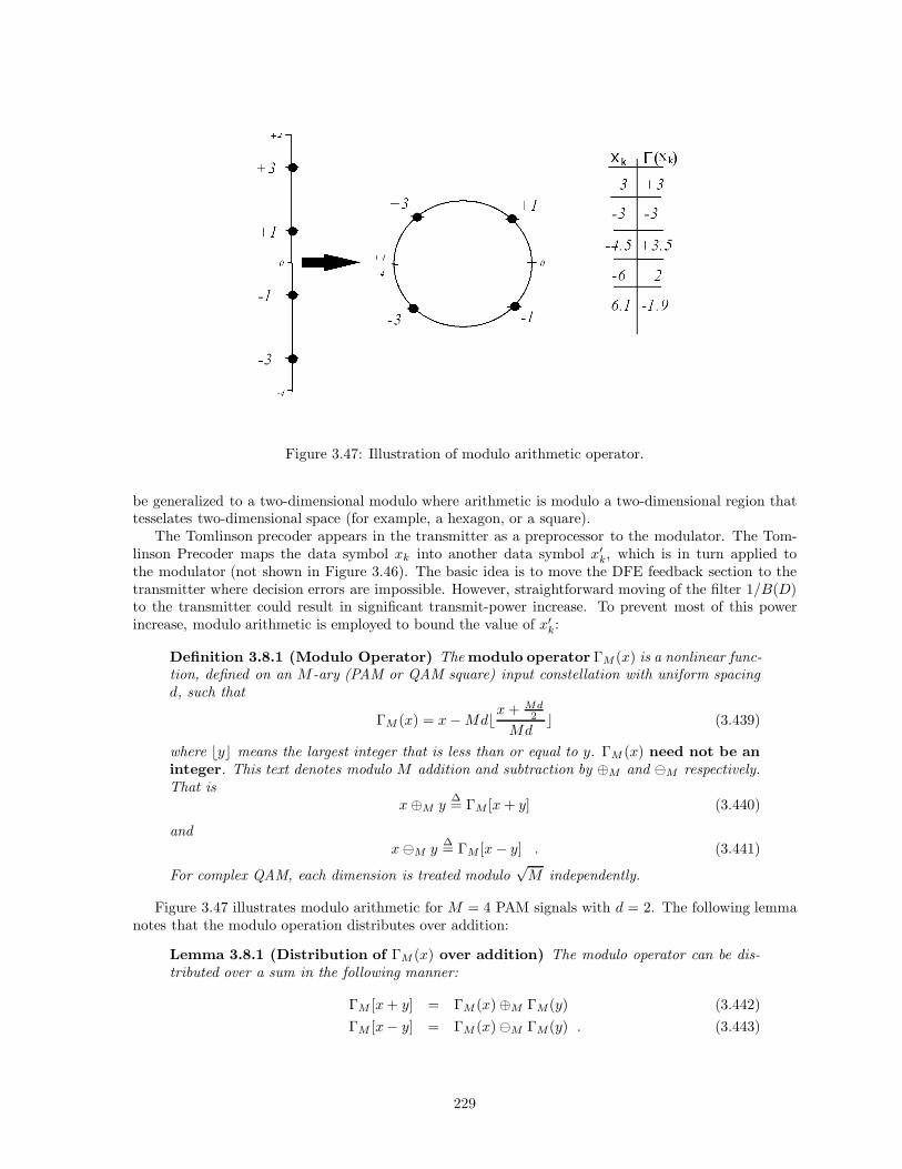
Figure 3.47: Illustration of modulo arithmetic operator.
be generalized to a two-dimensional modulo where arithmetic is modulo a two-dimensional region thattesselates two-dimensional space (for example, a hexagon, or a square).
The Tomlinson precoder appears in the transmitter as a preprocessor to the modulator. The Tom-linson Precoder maps the data symbol xk into another data symbol x′
k, which is in turn applied tothe modulator (not shown in Figure 3.46). The basic idea is to move the DFE feedback section to thetransmitter where decision errors are impossible. However, straightforward moving of the filter 1/B(D)to the transmitter could result in significant transmit-power increase. To prevent most of this powerincrease, modulo arithmetic is employed to bound the value of x′
k:
Definition 3.8.1 (Modulo Operator) The modulo operator ΓM (x) is a nonlinear func-tion, defined on an M -ary (PAM or QAM square) input constellation with uniform spacingd, such that
ΓM (x) = x − Mdbx + Md
2
Mdc (3.439)
where byc means the largest integer that is less than or equal to y. ΓM (x) need not be aninteger. This text denotes modulo M addition and subtraction by ⊕M and M respectively.That is
x ⊕M y∆= ΓM [x + y] (3.440)
andx M y
∆= ΓM [x − y] . (3.441)
For complex QAM, each dimension is treated modulo√
M independently.
Figure 3.47 illustrates modulo arithmetic for M = 4 PAM signals with d = 2. The following lemmanotes that the modulo operation distributes over addition:
Lemma 3.8.1 (Distribution of ΓM (x) over addition) The modulo operator can be dis-tributed over a sum in the following manner:
ΓM [x + y] = ΓM (x) ⊕M ΓM(y) (3.442)ΓM [x− y] = ΓM (x) M ΓM(y) . (3.443)
229
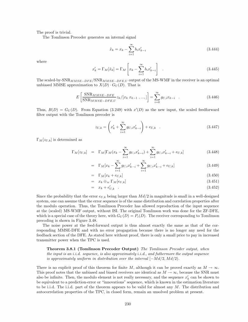
The proof is trivial.The Tomlinson Precoder generates an internal signal
xk = xk −∞∑
i=1
bix′k−i (3.444)
where
x′k = ΓM [xk] = ΓM
[xk −
∞∑
i=1
bix′k−i
]. (3.445)
The scaled-by-SNRMMSE−DFE/SNRMMSE−DFE,U output of the MS-WMF in the receiver is an optimalunbiased MMSE approximation to X(D) ·GU (D). That is
E
[SNRMMSE−DFE
SNRMMSE−DFE,Uzk/[xk xk−1 , ..., ]
]=
∞∑
i=0
gU,ixk−i . (3.446)
Thus, B(D) = GU(D). From Equation (3.249) with x′(D) as the new input, the scaled feedforwardfilter output with the Tomlinson precoder is
zU,k =
(x′
k +∞∑
i=1
gU,ix′k−i
)+ eU,k . (3.447)
ΓM [zU,k] is determined as
ΓM [zU,k] = ΓM [ΓM(xk −∞∑
i=1
gU,ix′k−i) +
∞∑
i=1
gU,ix′k−i + eU,k] (3.448)
= ΓM [xk −∞∑
i=1
gU,ix′k−i +
∞∑
i=1
gU,ix′k−i + eU,k] (3.449)
= ΓM [xk + eU,k] (3.450)= xk ⊕M ΓM [eU,k] (3.451)= xk + e′U,k . (3.452)
Since the probability that the error eU,k being larger than Md/2 in magnitude is small in a well-designedsystem, one can assume that the error sequence is of the same distribution and correlation properties afterthe modulo operation. Thus, the Tomlinson Precoder has allowed reproduction of the input sequenceat the (scaled) MS-WMF output, without ISI. The original Tomlinson work was done for the ZF-DFE,which is a special case of the theory here, with GU(D) = Pc(D). The receiver corresponding to Tomlinsonprecoding is shown in Figure 3.48.
The noise power at the feed-forward output is thus almost exactly the same as that of the cor-responding MMSE-DFE and with no error progagation because there is no longer any need for thefeedback section of the DFE. As stated here without proof, there is only a small price to pay in increasedtransmitter power when the TPC is used.
Theorem 3.8.1 (Tomlinson Precoder Output) The Tomlinson Precoder output, whenthe input is an i.i.d. sequence, is also approximately i.i.d., and futhermore the output sequenceis approximately uniform in distribution over the interval [−Md/2, Md/2).
There is no explicit proof of this theorem for finite M , although it can be proved exactly as M → ∞.This proof notes that the unbiased and biased receivers are identical as M → ∞, because the SNR mustalso be infinite. Then, the modulo element is not really necessary, and the sequence x′
k can be shown tobe equivalent to a prediction-error or “innovations” sequence, which is known in the estimation literatureto be i.i.d. The i.i.d. part of the theorem appears to be valid for almost any M . The distribution andautocorrelation properties of the TPC, in closed form, remain an unsolved problem at present.
230

Figure 3.48: Receiver for Tomlinson precoded MMSE-DFE implementation.
Using the uniform distribution assumption, the increase in transmit power for the TPC is from thenominal value of (M2−1)d2
12to the value for a continuous uniform random variable over the output interval
[−Md/2, Md/2), which is M2d2
12 , leading to an input power increase of
M2
M2 − 1(3.453)
for PAM and correspondinglyM
M − 1(3.454)
for QAM. When the input is not a square constellation, the Tomlinson Precoder Power loss is usuallylarger, but never more than a few dB. The number of nearest neighbors also increases to Ne = 2 for allconstellations. These losses can be eliminated (and actually a gain is possible) using techniques calledTrellis Precoding and/or shell mapping (See Section 10.6).
Laroia or Flexible Precoder
Figure 3.49 shows the Laroia precoder, which is a variation on Tomlinson precoding introduced byRajiv Laroia, mainly to reduce the transmit-power loss of the Tomlinson precoder. The Laroia precoderlargely preserves the shape of the transmitted constellation. The equivalent circuit is also shown inFigure 3.49 where the input is considered to be the difference between the actual input symbol value xk
and the “decision” output λk. The decision device finds the closest point in the infinite extension of theconstellation16. The extension of the constellation is the set of points that continue to be spaced by dminfrom the points on the edges of the original constellation and along the same dimensions as the originalconstellation. mk is therefore a small error signal that is uniform in distribution over (−d/2, d/2), thushaving variance d2/12 << Ex.
Because of the combination of channel and feedforward equalizer filters, the feedforward filter outputis
ZU (D) = [X(D) + M (D)] · GU (D) + EU (D) = X(D) − λ(D) + EU(D) . (3.455)
Processing ZU (D) by a decision operation leaves X(D)−λ(D), which essentially is the decision. However,to recover the input sequence X(D), the receiver forms
Z′(D) =X(D) − λ(D)
GU (D)= X(D) + M (D) . (3.456)
Since M (D) is uniform and has magnitude always less than d/2, then M (D) is removed by a secondtruncation (which is not really a decision, but operates using essentially the same logic as the firstdecision).
16The maximum range of such an infinite extension is actually the sum∑ν
i=1|< or =gU,i | · |Ree(D) or =xmax|.
231
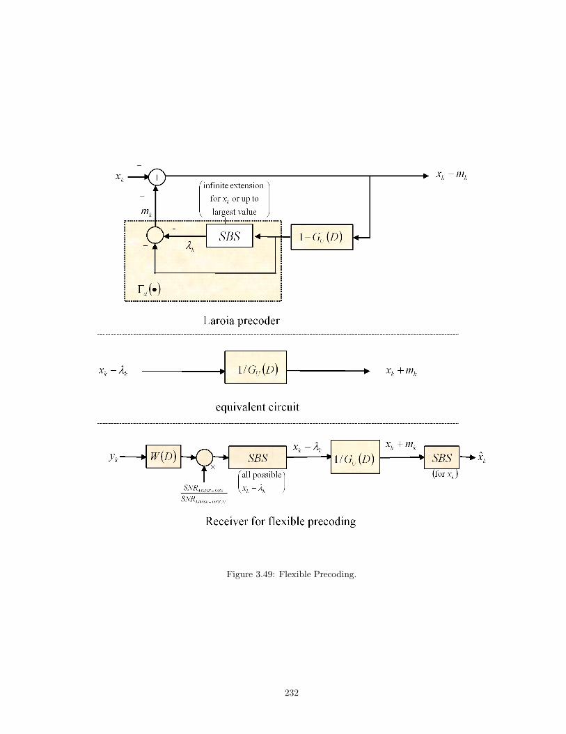
Figure 3.49: Flexible Precoding.
232

Figure 3.50: Flexible Precoding Example.
Example and error propagation in flexible precoding
EXAMPLE 3.8.1 (1 + .9D−1 system with flexible precoding) The flexible precoder andcorresponding receiver for the 1 + .9D−1 example appear in Figure 3.50. The bias removalfactor has been absorbed into all filters (7.85/6.85 multiples .633 to get .725 in feedbacksection, and multiplies .9469 to get 1.085 in feedforward section). The decision device isbinary in this case since binary antipodal transmission is used. Note the IIR filter in thereceiver. If an error is made in the first SBS in the receiver, then the magnitude of the erroris 2 = |+ 1− (−1)| = |− 1− (+1)|. Such an error is like an impulse of magnitude 2 added tothe input of the IIR filter, which has impulse response (−.725)k ·uk, producing a contributionto the correct sequence of 2 · (−.725)k ·uk. This produces an additional 1 error half the timeand an additional 2 errors 1/4 the time. Longer strings of errors will not occur. Thus, thebit and symbol error rate in this case increase by a factor of 1.5. (less than .1 dB loss).
A minor point is that the first decision in the receiver has an increased nearest neighborcoefficient of Ne = 1.5.
Generally speaking, when an error is made in the receiver for the flexible precoder,
(xk − λk) − decision(xk − λk) = ε · δk (3.457)
where ε could be complex for QAM. Then the designer needs to compute for each type of such error, itsprobability of occurence and then investigate the string (with (1/b)k being the impulse response of thepost-first-decision filter in the receiver)
|ε · (1/b)k| << dmin/2 . (3.458)
For some k, this relation will hold and that is the maximum burst length possible for the particular typeof error. Given the filter b is monic and minimum phase, this string should not be too long as long as the
233

roots are not too close to the unit circle. The single error may cause additional errors, but none of theseadditional errors in turn cause yet more errors (unlike a DFE where second and subsequent errors canlead to some small probability of infinite-length bursts), thus the probaility of an infinitely long burstis zero for the flexible precoder situation (or indeed any burst longer than the k that solves the aboveequation.
3.8.2 Partial Response Channel Models
Partial-response methods are a special case of precoding design where the ISI is forced to some knownwell-defined pattern. Receiver detectors are then designed for such partial-response channels directly,exploiting the known nature of the ISI rather than attempting to eliminate this ISI.
Classic uses of partial response abound in data transmission, some of which found very early use.For instance, the earliest use of telephone wires for data transmission inevitably found large intersymbolinterference because of a transformer that was used to isolate DC currents at one end of a phone linefrom those at the other (see Prob 3.35). The transformer did not pass low frequencies (i.e., DC), thusinevitably leading to non-Nyquist17 pulse shapes even if the phone line otherwise introduced no signficantintersymbol interference. Equalization may be too complex or otherwise undesirable as a solution, soa receiver can use a detector design that instead presumes the presence of a known fixed ISI. Anotherexample is magnetic recording (see Problem 3.36) where only flux changes on a recording surface can besensed by a read-head, and thus D.C. will not pass through the “read channel,” again inevitably leadingto ISI. Straightforward equalization is often too expensive at the very high speeds of magnetic-diskrecording systems.
Partial-Response (PR) channels have non-Nyquist pulse responses – that is, PR channels allow in-tersymbol interference – over a few (and finite number of) sampling periods. A unit-valued sample ofthe response occurs at time zero and the remaining non-zero response samples at subsequent samplingtimes, thus the name “partial response.” The study of PR channels is facilitated by mathematicallypresuming the tacit existence of a whitened matched filter, as will be described shortly. Then, a numberof common PR channels can be easily addressed.
Figure 3.51(a) illustrates the whitened-matched-filter. The minimum-phase equivalent of Figure3.51(b) exists if Q(D) = η0 ·H(D) ·H∗(D−∗) is factorizable.18 This chapter focuses on the discrete-timechannel and presumes the WMF’s presence without explicitly showing or considering it. The signaloutput of the discrete-time channel is
yk =∞∑
m=−∞hm · xk−m + nk , (3.459)
orY (D) = H(D) · X(D) + N (D) , (3.460)
where nk is sampled Gaussian noise with autocorrelation rnn,k = ‖p‖−2 · η−10 · N0
2 · δk or Rnn(D) =‖p‖−2 ·η−1
0 · N02 when the whitened-matched filter is used, and just denoted σ2
pr otherwise. In both cases,this noise is exactly AWGN with mean-square sample value σ2
pr, which is conveniently abbreviated σ2
for the duration of this chapter.
Definition 3.8.2 (Partial-Response Channel) A partial-response (PR) channel is anydiscrete-time channel with input/output relation described in (3.459) or (3.460) that also sat-isfies the following properties:
1. hk is finite-length and causal; hk = 0 ∀ k < 0 or k > ν, where ν < ∞ and is oftencalled the constraint length of the partial-response channel,
2. hk is monic; h0 = 1,
3. hk is minimum phase; H(D) has all ν roots on or outside the unit circle,
17That is, they do not satisfy Nyquist’s condition for nonzero ISI - See Chapter 3, Section 3.18H(D) = Pc(D) in Section 3.6.3 on ZF-DFE.
234

Figure 3.51: Minimum Phase Equivalent Channel.;’
4. hk has all integer coefficients; hk ∈ Z ∀ k 6= 0 (where Z denotes the set of integers).
More generally, a discrete finite-length channel satisfying all properties above except the lastrestriction to all integer coefficients is known as a controlled intersymbol-interferencechannel.
Controlled ISI and PR channels are a special subcase of all ISI channels, for which hk = 0 ∀ k > ν. ν isthe constraint length of the controlled ISI channel. Thus, effectively, the channel can be modeled asan FIR filter, and hk is the minimum-phase equivalent of the sampled pulse response of that FIR filter.The constraint length defines the span in time νT of the non-zero samples of this FIR channel model.
The controlled ISI polynomial (D-transform)19 for the channel simplifies to
H(D) ∆=ν∑
m=0
hmDm , (3.461)
where H(D) is always monic, causal, minimum-phase, and an all-zero (FIR) polynomial. If the receiverprocesses the channel output of an ISI-channel with the same whitened-matched filter that occurs inthe ZF-DFE of Section 3.6, and if Pc(D) (the resulting discrete-time minimum-phase equivalent channelpolynomial when it exists) is of finite degree ν, then the channel is a controlled intersymbol interferencechannel with H(D) = Pc(D) and σ2 = N0
2 · ‖p‖−2 ·η−10 . Any controlled intersymbol-interference channel
is in the form that the Tomlinson Precoder of Section 3.8.1 could be used to implement symbol-by-symbol detection on the channel output. As noted in Section 3.8.1, a (usually small) transmit symbolenergy increase occurs when the Tomlinson Precoder is used. Section 3.8.4 shows that this loss can beavoided for the special class of polynomials H(D) that are partial-response channels.
19The D-Transform of FIR channels (ν < ∞) is often called the “channel polynomial,” rather than its “D-Transform”in partial-response theory. This text uses these two terms interchangeably.
235

Figure 3.52: Simple DFE for some partial-response channels.
Equalizers for the Partial-response channel.
This small subsection serves to simplify and review equalization structure on the partial-response channel.The combination of integer coefficients and minimum-phase constraints of partial-response channels
allows a very simple implementation of the ZF-DFE as in Figure 3.52. Since the PR channel is alreadydiscrete time, no sampling is necessary and the minimum-phase characteristic of H(D) causes the WMFof the ZF-DFE to simplify to a combined transfer function of 1 (that is, there is no feedforward sec-tion because the channel is already minimum phase). The ZF-DFE is then just the feedback sectionshown, which easily consists of the feedback coefficients −hm for the delayed decisions corresponding toxk−m, m = 1, ..., ν. The loss with respect to the matched filter bound is trivially 1/‖H‖2, which is easilycomputed as 3 dB for H(D) = 1±Dν (any finite ν) with simple ZF-DFE operation zk = yk − xk−ν and6 dB for H(D) = 1 + D − D2 − D3 with simple ZF-DFE operation zk = yk − xk−1 + xk−2 + xk−3.
The ZF-LE does not exist if the channel has a zero on the unit circle, which all partial-responsechannels do. A MMSE-LE could be expected to have signficant noise enhancement while existing.The MMSE-DFE will perform slightly better than the ZF-DFE, but is not so easy to compute as thesimple DFE. Tomlinson or Flexible precoding could be applied to eliminate error propagation for a smallincrease in transmit power ( M2
M2−1).
3.8.3 Classes of Partial Response
A particularly important and widely used class of partial response channels are those with H(D) givenby
H(D) = (1 + D)l (1 − D)n , (3.462)
where l and n are nonnegative integers.For illustration, Let l = 1 and n = 0 in (3.462), then
H(D) = 1 + D , (3.463)
236

Figure 3.53: Transfer Characteristic for Duobinary signaling.
which is sometimes called a “duobinary” channel (introduced by Lender in 1960). The Fourier transformof the duobinary channel is
H(e−ωT ) = H(D)|D=e−ωT = 1 + e−ωT = 2e−ωT/2 · cos(
ωT
2
). (3.464)
The transfer function in (3.464) has a notch at the Nyquist Frequency and is generally “lowpass” inshape, as is shown in Figure 3.53. A discrete-time ZFE operating on this channel would produce infinitenoise enhancement. If SNRMFB = 16 dB for this channel, then
Q(e−ωT ) +1
SNRMFB= (1 + 1/40) + cos ωT . (3.465)
The MMSE-LE will have performance (observe that N02 = .05)
σ2MMSE−LE =
N0
2T
2π
∫ πT
− πT
1‖p‖2(1.025 + cos ωT )
dω =N0
21/2√
1.0252 − 12= 2.22
N0
2, (3.466)
The SNRMMSE−LE,U is easily computed to be 8 (9dB), so the equalizer loss is 7 dB in this case. Forthe MMSE-DFE, Q(D) + 1
SNRMFB= 1.025
1.64(1 + .8D)(1 + .8D−1), so that γ0 = 1.025/1.64 = .625, and
thus γMMSE-DFE = 2.2dB. For the ZF-DFE, η0 = 12 , and thus γZF-DFE = 3dB.
It is possible to achieve MFB performance on this channel with complexity far less than any equalizerstudied earlier in this chapter, as will be shown in Chapter 9. It is also possible to use a precoder withno transmit power increase to eliminate the error-propagation-prone feedback section of the ZF-DFE.
There are several specific channels that are used in practice for partial-response detection:
EXAMPLE 3.8.2 (Duobinary 1 + D) The duobinary channel (as we have already seen)has
H(D) = 1 + D . (3.467)
237

The frequency response was already plotted in Figure 3.53. This response goes to zero at theNyquist Frequency, thus modeling a lowpass-like channel. For a binary input of xk = ±1,the channel output (with zero noise) takes on values ±2 with probability 1/4 each and 0 withprobability 1/2. In general, for M -level inputs (±1 ± 3 ± 5 ... ± (M − 1)), there are 2M − 1possible output levels, −2M + 2, ..., 0, ..., 2M − 2. These output values are all possiblesums of pairs of input symbols.
EXAMPLE 3.8.3 (DC Notch 1 − D) The DC Notch channel has
H(D) = 1 − D , (3.468)
so that l = 0 and n = 1 in (3.462). The frequency response is
H(e−ωT ) = 1 − e−ωT = 2e−ω T2 · sin ωT
2. (3.469)
The response goes to zero at the DC (ω = 0), thus modeling a highpass-like channel. Fora binary input of xk = ±1, the channel output (with zero noise) takes on values ±2 withprobability 1/4 each and 0 with probability 1/2. In general for M -level inputs (±1 ± 3 ±5 ... ± (M − 1)), there are 2M − 1 possible output levels, −2M + 2, ..., 0, ..., 2M − 2.
When the 1 − D shaping is imposed in the modulator itself, rather than by a channel, thecorresponding modulation is known as AMI (Alternate Mark Inversion) if a differentialencoder is also used as shown later in this section. AMI modulation prevents “charge” (DC)from accumulating and is sometimes also called “bipolar coding,” although the use of thelatter term is often confusing because bipolar transmission may have other meanings for somecommunications engineers. AMI coding, and closely related methods are used in multiplexedT1 (1.544 Mbps DS1 or “ANSI T1.403”) and E1 (2.048 Mbps or “ITU-T G.703”) speeddigital data transmission on twisted pairs or coaxial links. These signals were once prevalentin telephone-company non-fiber central-office transmission of data between switch elements.
EXAMPLE 3.8.4 (Modified Duobinary 1 − D2) The modified duobinary channel has
H(D) = 1 − D2 = (1 + D)(1 − D) , (3.470)
so l = n = 1 in (3.462). Modified Duobinary is sometimes also called “Partial ResponseClass IV” or PR4 or PRIV in the literature. The frequency response is
H(e−ωT ) = 1 − e−ω2T = 2e−ωT · sin(ωT ) . (3.471)
The response goes to zero at the DC (ω = 0) and at the Nyquist frequency (ω = π/T ),thus modeling a bandpass-like channel. For a binary input of xk = ±1, the channel output(with zero noise) takes on values ±2 with probability 1/4 each and 0 with probability 1/2.In general, for M -level inputs (±1 ± 3 ± 5 ... ± (M − 1)), there are 2M − 1 possibleoutput levels. Modified duobinary is equivalent to two interleaved 1 − D channels, eachindependently acting on the inputs corresponding to even (odd) time samples, respectively.Many commercial disk drives use PR4.
EXAMPLE 3.8.5 (Extended Partial Response 4 and 6 (1 + D)l(1 − D)n) The EPR4channel has l = 2 and n = 1 or
H(D) = (1 + D)2(1 − D) = 1 + D − D2 − D3 . (3.472)
This channel is called EPR4 because it has 4 non-zero samples (Thapar). The frequencyresponse is
H(e−ωT ) = (1 + e−ωT )2(1 − e−ωT ) . (3.473)
238

Figure 3.54: Transfer Characteristic for EPR4 and EPR6
The EPR6 channel has l = 4 and n = 1 (6 nonzero samples)
H(D) = (1 + D)4(1 − D) = 1 + 3D + 2D2 − 2D3 − 3D4 − D5 . (3.474)
The frequency response is
H(e−ωT ) = (1 + e−ωT )4(1 − e−ωT ) . (3.475)
These 2 channels, along with PR4, are often used to model disk storage channels in magneticdisk or tape recording. The response goes to zero at DC (ω = 0) and at the Nyquist frequencyin both EPR4 and EPR6, thus modeling bandpass-like channels. The magnitude of these twofrequency characteristics are shown in Figure 3.54. These are increasingly used in commercialdisk storage read detectors.
The higher the l, the more “lowpass” in nature that the EPR channel becomes, and the more appropriateas bit density increases on any given disk.
For partial-response channels, the use of Tomlinson Precoding permits symbol-by-symbol detection,but also incurs an M2/(M2 − 1) signal energy loss for PAM (and M/(M − 1) for QAM). A simplermethod for PR channels, that also has no transmit energy penalty, is known simply as a “precoder.”
3.8.4 Simple Precoding
The simplest form of precoding for the duobinary, DC-notch, and modified duobinary partial-responsechannels is the so-called “differential encoder.” The message at time k, mk, is assumed to take onvalues m = 0, 1, ..., M − 1. The differential encoder for the case of M = 2 is most simply described asthe device that observes the input bit stream, and changes its output if the input is 1 and repeats thelast output if the input is 0. Thus, the differential encoder input, mk, represents the difference (or sum)between adjacent differential encoder output (mk and mk−1) messages20:
20This operation is also very useful even on channels without ISI, as an unknown inversion in the channel (for instance,an odd number of amplifiers) will cause all bits to be in error if (differential) precoding is not used.
239

Figure 3.55: Precoded Partial Response Channel.
Definition 3.8.3 (Differential Encoder) Differential encoders for PAM or QAM mod-ulation obey one of the two following relationships:
mk = mk mk−1 (3.476)mk = mk ⊕ mk−1 , (3.477)
where represents subtraction modulo M (and ⊕ represents addition modulo M). For SQQAM, the modulo addition and subtraction are performed independently on each of the twodimensions, with
√M replacing M . (A differential phase encoder is also often used for QAM
and is discussed later in this section.)
A differential encoder is shown on the left side of Figure 3.55. As an example if M = 4 the correspondinginputs and outputs are given in the following table:mk - 3 1 0 2 1 0 3mk 0 3 2 2 0 1 3 0k -1 0 1 2 3 4 5 6With either PAM or QAM constellations, the dimensions of the encoder output mk are converted
into channel input symbols (±d2 , ±3d
2 ...) according to
xk = [2mk − (M − 1)]d
2. (3.478)
Figure 3.55 illustrates the duobinary channel H(D) = 1 + D, augmented by the precoding operationof differential encoding as defined in (3.476). The noiseless minimum-phase-equivalent channel outputyk is
yk = xk + xk−1 = 2(mk + mk−1)d
2− 2(M − 1)
d
2(3.479)
so21
yk
d+ (M − 1) = mk + mk−1 (3.480)
21(•)M means the quantity is computed in M -level arithmetic, for instance, (5)4 = 1. Also note that ΓM(x) 6= (x)M ,and therefore ⊕ is different from the ⊕M of Section 3.5. The functions (x)M and ⊕ have strictly integer inputs and havepossible outputs 0, ...,M − 1 only.
240
([yk
d+ (M − 1)
])
M
= mk ⊕ mk−1 (3.481)([
yk
d+ (M − 1)
])
M
= mk (3.482)
where the last relation (3.482) follows from the definition in (3.476). All operations are integer mod-M .Equation (3.482) shows that a decision on yk about mk can be made without concern for preceding orsucceeding yk, because of the action of the precoder. The decision boundaries are simply the obviousregions symmetrically placed around each point for a memoryless ML detector of inputs and the decodingrules for M = 2 and M = 4 are shown in Figure 3.55. In practice, the decoder observes yk, not yk, sothat yk must first be quantized to the closest noise-free level of yk. That is, the decoder first quantizesyk to one of the values of (−2M + 2)(d/2), ..., (2M − 2)(d/2). Then, the minimum distance between
outputs is dmin = d, so thatdmin2σpr
= d2σpr
, which is 3 dB below the√
MFB =√
2σpr
(d/2) for the 1 + D
channel because ‖p‖2 = 2. (Again, σ2pr = ‖p‖−2 · η−1
0 · N02 with a WMF and otherwise is just σ2
pr.) Thisloss is identical to the loss in the ZF-DFE for this channel. One may consider the feedback section of theZF-DFE as having been pushed through the linear channel back to the transmitter, where it becomesthe precoder. With some algebra, one can show that the TPC, while also effective, would produce a4-level output with 1.3 dB higher average transmit symbol energy for binary inputs. The output levelsare assumed equally likely in determining the decision boundaries (half way between the levels) eventhough these levels are not equally likely.
The precoded partial-response system eliminates error propagation, and thus has lower Pe than theZF-DFE. This elimination of error propagation can be understood by investigating the nearest neighborcoefficient for the precoded situation in general. For the 1 + D channel, the (noiseless) channel outputlevels are −(2M − 2) − (2M − 4)... 0 ... (2M − 4) (2M − 2) with probabilities of occurrence 1
M22
M2 ...MM2 ... 2
M21
M2 , assuming a uniform channel-input distribution. Only the two outer-most levels have onenearest neighbor, all the rest have 2 nearest neighbors. Thus,
Ne =2
M2(1) +
M2 − 2M2
(2) = 2(
1 − 1M2
). (3.483)
For the ZF-DFE, the input to the decision device zk as
zk = xk + xk−1 + nk − xk−1 , (3.484)
which can be rewrittenzk = xk + (xk−1 − xk−1) + nk . (3.485)
Equation 3.485 becomes zk = xk + nk if the previous decision was correct on the previous symbol.However, if the previous decision was incorrect, say +1 was decided (binary case) instead of the correct−1, then
zk = xk − 2 + nk , (3.486)
which will lead to a next-symbol error immediately following the first almost surely if xk = 1 (and noerror almost surely if xk = −1). The possibility of zk = xk + 2 + nk is just as likely to occur and followsan identical analysis with signs reversed. For either case, the probability of a second error propagatingis 1/2. The other half of the time, only 1 error occurs. Half the times that 2 errors occur, a third erroralso occurs, and so on, effectively increasing the error coefficient from Ne = 1 to
Ne = 2 = 1(12) + 2(
14) + 3(
18) + 4(
116
) + ... =∞∑
k=1
k · (.5)k =.5
(1 − .5)2. (3.487)
(In general, the formula∑∞
k=1 k · rk = r(1−r)2 , r < 1 may be useful in error propagation analysis.) The
error propagation can be worse in multilevel PAM transmission, when the probability of a second erroris (M − 1)/M , leading to
Ne(error prop)Ne(no error prop)
= 1 · 1M
+ 2 · M − 1M
· 1M
+ 3 ·(
M − 1M
)2
· 1M
+ ... (3.488)
241
=∞∑
k=1
k ·(
M − 1M
)k−1
· 1M
(3.489)
= M . (3.490)
Precoding eliminates this type of error propagation, although Ne increases by a factor22 of (1 + 1/M )with respect to the case where no error propagation occurred.
For the ZF-DFE system, Pe = 2(M − 1)Q( d2σpr
), while for the precoded partial-response system,Pe = 2
(1 − 1
M2
)Q( d
2σpr). For M ≥ 2, the precoded system always has the same or fewer nearest
neighbors, and the advantage becomes particularly pronounced for large M . Using a rule-of-thumbthat a factor of 2 increase in nearest neighbors is equivalent to an SNR loss of .2 dB (which holds atreasonable error rates in the 10−5 to 10−6 range), the advantage of precoding is almost .2 dB for M = 4.For M = 8, the advantage is about .6 dB, and for M = 64, almost 1.2 dB. Precoding can be simplerto implement than a ZF-DFE because the integer partial-response channel coefficients translate readilyinto easily realized finite-field operations in the precoder, while they represent full-precision add (andshift) operations in feedback section of the ZF-DFE.
Precoding the DC Notch or Modified Duobinary Channels
The mk = mk mk−1 differential encoder works for the 1 + D channel. For the 1 − D channel, theequivalent precoder is
mk = mk ⊕ mk−1 , (3.491)
which is sometimes also called NRZI (non-return-to-zero inverted) precoding, especially by storage-channel engineers. In the 1 − D case, the channel output is
yk = xk − xk−1 = 2(mk − mk−1)d
2(3.492)
yk
d= mk − mk−1 (3.493)
(yk
d
)
M
= mk mk−1 (3.494)(
yk
d
)
M
= mk . (3.495)
The minimum distance and number of nearest neighbors are otherwise identical to the 1 + D case juststudied, as is the improvement over the ZF-DFE. The 1−D2 case is identical to the 1−D case, on twointerleaved 1 − D channels at half the rate. The overall precoder for this situation is
mk = mk ⊕ mk−2 , (3.496)
and the decision rule is (yk
d
)
M
= mk . (3.497)
The combination of precoding with the 1 − D channel is often called “alternate mark inversion (AMI)”because each successive transmitted “1” bit value causes a nonzero channel output amplitude of polarityoppositie to the last nonzero channel output amplitude, while a “0” bit always produces a 0 level at thechannel output.
Precoding EPR4
An example of precoding for the extended Partial Response class is EPR4, which has l = 2 and n = 1in (3.472), or EPR4. Then,
yk = xk + xk−1 − xk−2 − xk−3 (3.498)22The ratio of 2(1− 1/M2) with precoding to 2(1− 1/M) for M-ary PAM with no error propagation effects included
242

yk = d(mk + mk−1 − mk−2 − mk−3) (3.499)yk
d= mk + mk−1 − mk−2 − mk−3 (3.500)
(yk
d
)
M
= mk ⊕ mk−1 mk−2 mk−3 (3.501)(
yk
d
)
M
= mk (3.502)
where the precoder, from (3.502) and (3.501), is
mk = mk mk−1 ⊕ mk−2 ⊕ mk−3 . (3.503)
The minimum distance at the channel output is still d in this case, so Pe ≤ Ne · Q(d/2σpr), but theMFB = ( d
σpr)2, which is 6dB higher. The same 6dB loss that would occur with an error-propagation-free
ZF-DFE on this channel.For the 1 + D − D2 − D3 channel, the (noiseless) channel output levels are −(4M − 4) − (4M −
6)... 0 ... (4M −6) (4M −4). Only the two outer-most levels have one nearest neighbor, all the rest have2 nearest neighbors. Thus,
Ne =2
M4(1) +
M4 − 2M4
(2) = 2(
1 − 1M4
). (3.504)
Thus the probability of error for the precoded system is Pe = 2(1 − 1
M4
)Q( 1
σpr). The number of nearest
neighbors for the ZF-DFE, due to error propagation, is difficult to compute, but clearly will be worse.
3.8.5 General Precoding
The general partial response precoder can be extrapolated from previous results:
Definition 3.8.4 (The Partial-Response Precoder) The partial-response precoderfor a channel with partial-response polynomial H(D) is defined by
mk = mk
ν⊕
i=1
(−hi) · mk−i . (3.505)
The notation⊕
means a mod-M summation, and the multiplication can be performed withoutambiguity because the hi and mk−i are always integers.
The corresponding memoryless decision at the channel output is
mk =
(yk
d+
ν∑
i=0
hi
(M − 1
2
))
M
. (3.506)
The reader should be aware that while the relationship in (3.505) is general for partial-response channels,the relationship can often simplify in specific instances, for instance the precoder for “EPR5,” H(D) =(1 + D)3(1 − D) simplifies to mk = mk ⊕ mk−4 when M = 2.
In a slight abuse of notation, engineers often simplify the representation of the precoder by simplywriting it as
P(D) =1
H(D)(3.507)
where P(D) is a polynomial in D that is used to describe the “modulo-M” filtering in (3.505). Of course,this notation is symbolic. Furthermore, one should recognize that the D means unit delay in a finitefield, and is therefore a delay operator only – one cannot compute the Fourier transform by insertingD = e−ωT into P(D); Nevertheless, engineers commonly to refer to the NRZI precoder as a 1/(1 ⊕ D)precoder.
243

Lemma 3.8.2 (Memoryless Decisions for the Partial-Response Precoder) The partial-response precoder, often abbreviated by P(D) = 1/H(D), enables symbol-by-symbol decodingon the partial-response channel H(D). An upper bound on the performance of such symbol-by-symbol decoding is
Pe ≤ 2(
1 − 1Mν+1
)Q
[d
2σpr
], (3.508)
where d is the minimum distance of the constellation that is output to the channel.
Proof: The proof follows by simply inserting (3.505) into the expression for yk and simpli-fying to cancel all terms with hi, i > 0. The nearest-neighbor coefficient and d/2σpr followtrivially from inspection of the output. Adjacent levels can be no closer than d on a partial-response channel, and if all such adjacent levels are assumed to occur for an upper bound onprobability of error, then the Pe bound in (3.508) holds. QED.
3.8.6 Quadrature PR
Differential encoding of the type specified earlier is not often used with QAM systems, because QAMconstellations usually exhibit 90o symmetry. Thus a 90o offset in carrier recovery would make theconstellation appear exactly as the original constellation. To eliminate the ambiguity, the bit assignmentfor QAM constellations usually uses a precoder that uses the four possibilities of the most-significant bitsthat represent each symbol to specify a phase rotation of 0o, 90o, 180o, or 270o with respect to the lastsymbol transmitted. For instance, the sequence 01, 11, 10, 00 would produce (assuming an initial phaseof 0o, the sequence of subsequent phases 90o, 0o, 180o, and 180o. By comparing adjacent decisions andtheir phase difference, these two bits can be resolved without ambiguity even in the presence of unknownphase shifts of multiples of 90o. This type of encoding is known as differential phase encoding andthe remaining bits are assigned to points in large M QAM constellations so that they are the same forpoints that are just 90o rotations of one another. (Similar methods could easily be derived using 3 ormore bits for constellations with even greater symmetry, like 8PSK.)
Thus the simple precoder for the 1 + D and 1 − D (or 1 − D2) given earlier really only is practicalfor PAM systems. The following type of precoder is more practical for these channels:
A Quadrature Partial Response (QPR) situation is specifically illustrated in Figure 3.56 for M = 4or b = 1 bit per dimension. The previous differential encoder could be applied individually to bothdimensions of this channel, and it could be decoded without error. All previous analysis is correct,individually, for each dimension. There is, however, one practical problem with this approach: If thechannel were to somehow rotate the phase by ±90o (that is, the carrier recovery system locked on thewrong phase because of the symmetry in the output), then there would be an ambiguity as to which partwas real and which was imaginary. Figure 3.56 illustrates the ambiguity: the two messages (0, 1) = 1and (1, 0) = 2 commute if the channel has an unknown phase shift of ±90o. No ambiguity exists foreither the message (0, 0) = 0 or the message (1, 1) = 3. To eliminate the ambiguity,the precoder encodesthe 1 and 2 signals into a difference between the last 1 (or 2) that was transmitted. This precoder thusspecifies that an input of 1 (or 2) maps to no change with respect to the last input of 1 (or 2), while aninput of 2 maps to a change with respect to the last input of 1 or 2.
A precoding rule that will eliminate the ambiguity is then
Rule 3.8.1 (Complex Precoding for the 1+D Channel) if mk = (mi,k, mq,k) = (0, 0) or (1, 1)then
mi,k = mi,k ⊕ mi,k−1 (3.509)mq,k = mq,k ⊕ mq,k−1 (3.510)
else if mk = (mi,k, mq,k) = (0, 1) or (1, 0), check the last m = (0, 1) or (1, 0) transmitted,call it m90, (that is, was m90 = 1 or 2 ?). If m90 = 1, the precoder leaves mk unchangedprior to differential encoding according to (3.509) and (3.510). The operations ⊕ and arethe same in binary arithmetic.
244

Figure 3.56: Quadrature Partial Response Example with 1 + D.
245

If m90 = 2, then the precoder changes mk from 1 to 2 (or from 2 to 1) prior to encodingaccording to (3.509) and (3.510).
The corresponding decoding rule is (keeping a similar state y90 = 1, 2 at the decoder)
mk =
(0, 0) yk = [ ±2 ± 2 ](1, 1) yk = [ 0 0 ](0, 1) (yk = [ 0 ± 2 ] or yk = [ ±2 0 ]) and 6 yk − 6 y90 = 0(1, 0) (yk = [ 0 ± 2 ] or yk = [ ±2 0 ]) and 6 yk − 6 y90 6= 0
. (3.511)
The probability of error and minimum distance are the same as was demonstrated earlier for this typeof precoder, which only resolves the 90o ambiguity, but is otherwise equivalent to a differential encoder.There will however be limited error propagation in that one detection error on the 1 or 2 message pointsleads to two decoded symbol errors on the decoder output.
246

Figure 3.57: Basic diversity channel model.
3.9 Diversity Equalization
Diversity in transmission is the use of multiple channels from a single message source to several receivers,as illustrated in Figure 3.57. Optimally, the principles of Chapter 1 apply directly where the conditionalprobability distribution py/x of the channel has a larger dimensionality on the channel output y than onthe input, x, Ny > Nx. Often, this diversity leads to a lower probability of error for the same message,mainly because a greater channel-output minimum distance between possible (noiseless) output datasymbols can be achieved with a larger number of channel output dimensions. However, intersymbolinterference between successive transmissions, along with interference between the diversity dimensions,again can lead to a potentially complex optimum receiver and detector. Thus, equalization again allowsproductive use of suboptimal SBS detectors. The equalizers in the case of diversity become matrixequivalents of those studied in Sections 3.5 - 3.7.
3.9.1 Multiple Received Signals and the RAKE
Figure 3.57 illustrates the basic diversity channel. Channel outputs caused by the same channel inputhave labels yl(t), l = 0, ..., L− 1. These channel outputs can be created intentionally by retransmissionof the same data symbols at different times and/or (center) frequencies. Spatial diversity often occurs inwireless transmission where L spatially separated antennas may all receive the same transmitted signal,but possibly with different filtering and with noises that are at least partially independent.
With each channel output following the model
yp,l(t) =∑
k
xkpl(t − kT ) + nl(t) , (3.512)
247
a corresponding L × 1 vector channel description is
yp(t) =∑
k
xkp(t − kT ) + np(t) , (3.513)
where
yp(t) ∆=
y0(t)y1(t)
...yL−1(t)
p(t) ∆=
p0(t)p1(t)
...pL−1(t)
and np(t) ∆=
n0(t)n1(t)
...nL−1(t)
. (3.514)
The generalization of an inner product is readily seen to be
< x(t), y(t) >=∑
i
∫ ∞
−∞xi(t)y∗i (t)dt . (3.515)
Without loss of generality, the noise can be considered to be white on each of the L diversity channels,independent of the other diversity channels, and with equal power spectral densities N0
2.23
A single transmission of x0 corresponds to a vector signal
yp(t) = x0 · p(t) + n(t) = x0 · ‖p‖ · ϕp(t) + n(t) . (3.516)
This situation generalizes slightly that considered in Chapter 1, where matched-filter demodulatorsthere combined all time instants through integration, a generalization of the inner product’s usual sumof products. A matched filter in general simply combines the signal components from all dimensionsthat have independent noise. Here, that generalization of combination simply needs to include also thecomponents corresponding to each of the diversity channels so that all signal contributions are summedto create maximum signal-to-noise ratio. The relative weighting of the different diversity channels is thusmaintained through L unnormalized parallel matched filters each corresponding to one of the diversitychannels. When several copies are combined across several diversity channels or new dimensions (whethercreated in frequency, long delays in time, or space), the combination is known as the RAKE matchedfilter of Figure 3.58:
Definition 3.9.1 (RAKE matched filter) A RAKE matched filter is a set of parallelmatched filters each operating on one of the diversity channels in a diversity transmissionsystem that is followed by a summing device as shown in Figure 3.58. Mathematically, theoperation is denoted by
yp(t) =L−1∑
l=0
p∗l (−t) ∗ yl(t) . (3.517)
The RAKE was originally so named by Green and Price in 1958 because of the analogy of the variousmatched filters being the “fingers” of a garden rake and the sum corresponding to the collection of thefingers at the rake’s pole handle, nomenclature thus often being left to the discretion of the inventor,however unfortunate for posterity. The RAKE is sometimes also called a diversity combiner, althoughthe latter term also applies to other lower-performance suboptimal combining methods that do notmaximize overall signal to noise strength through matched filter. One structure, often called maximalcombining, applies a matched filter only to the strongest of the L diversity paths to save complexity.The equivalent channel for this situation is then the channel corresponding to this maximum-strengthindividual path. The original RAKE concept was conceived in connection with a spread-spectrumtransmission method that achieves diversity essentially in frequency (but more precisely in a code-division dimension to be discussed in the appendix of Chapter 5), but the matched filtering implied is
23In practice, the noises may be correlated with each other on different subchannels and not white with covariance matrix
Rn(t) and power spectral density matrix Rn(f) = N02
· R1/2n (f)R
∗/2n (f). By prefiltering the vector channel output by the
matrix filter R−1/2n (f), the noise will be whitened and the noise equivalentmatrix channel becomes P (f) → R
−1/2n (f)P (f).
Anaylsis with the equivalent channel can then proceed as if the noise where white, independent on the diversity channels,and of the same variance N0
2on all.
248

Figure 3.58: The basic RAKE matched filter combiner.
easily generalized. Some of those who later studied diversity combining were not aware of the connectionto the RAKE and thus the multiple names for the same structure, although diversity combining is amore accurate name for the method.
This text also defines rl (t) = pl(t) ∗ p∗l (−t) and
r(t) =L−1∑
l=0
rl(t) (3.518)
for an equivalent RAKE-output equivalent channel and the norm
‖p‖2 =L−1∑
l=0
‖pl‖2 . (3.519)
Then, the normalized equivalent channel q(t) is defined through
r(t) = ‖p‖2 · q(t) . (3.520)
The sampled RAKE output has D-transform
Y (D) = X(D) · ‖p‖2 · Q(D) + N (D) , (3.521)
which is essentially the same as the early channel models used without diversity except for the additionalscale factor of ‖p‖2, which also occurs in the noise autcorrelation, which is
Rnn(D) =N0
2· ‖p‖2 · Q(D) . (3.522)
An SNRMFB = Ex‖p‖2
N02
and all other detector and receiver principles previously developed in this
text now apply directly.
3.9.2 Infinite-length MMSE Equalization Structures
The sampled RAKE output can be scaled by the factor ‖p‖−1 to obtain a model identical to that foundearlier in Section 3.1 in Equation (3.26) with Q(D) and ‖p‖ as defined in Subsection 3.9.1. Thus, the
249

MMSE-DFE, MMSE-LE, and ZF-LE/DFE all follow exactly as in Sections 3.5 -3.7. The matched-filterbound SNR and each of the equalization structures tend to work better with diversity because ‖p‖2 istypically larger on the equivalent channel created by the RAKE. Indeed the RAKE will work betterthan any of the individual channels, or any subset of the diversity channels, with each of the equalizerstructures.
Often while one diversity channel has severe characteristics, like an inband notch or poor transmissioncharacteristic, a second channel is better. Thus, diversity systems tend to be more robust.
EXAMPLE 3.9.1 (Two ISI channels in parallel) Figure 3.59 illustrates two diversitychannels with the same input and different intersymbol interference. The first upper channelhas a sampled time equivalent of 1 + .9D−1 with noise variance per sample of .181 (andthus could be the channel consistently examined throughout this Chapter so Ex = 1). Thischannel is in effect anti-causal (or in reality, the .9 comes first). A second channel has causalresponse 1 + .8D with noise variance .164 per sample and is independent of the noise inthe first channel. The ISI effectively spans 3 symbol periods among the two channels at acommon receiver that will decide whether xk = ±1 has been transmitted.
The SNRMFB for this channel remains SNRMFB = Ex·‖p‖2
N02
, but it remains to compute
this quantity correctly. First the noise needs to be whitened. While the two noises areindependent, they do not have the same variance per sample, so a pre-whitening matrix is
[1 0
0√
.181
.164
](3.523)
and so then the energy quantified by ‖p‖2 is
‖p‖2 = ‖p1‖2 + ‖p2‖2 = 1.81 +(
.181
.164
)1.64 = 2(1.81) . (3.524)
ThenSNRMFB =
1 · 2(1.81).181
= 13 dB . (3.525)
Because of diversity, this channel has a higher potential performance than the single channelalone. Clearly having a second look at the input through another channel can’t hurt (evenif there is more ISI now). The ISI is characterized as always by Q(D), which in this case is
Q(D) =1
2(1.81)
[(1 + .9D−1)(1 + .9D) +
.181
.164(1 + .8D)(1 + .8D−1)
](3.526)
= .492D + 1 + .492D−1 (3.527)= .7082 · (1 + .835D) · (1 + .835D−1) (3.528)
Q(D) = .492D + (1 + 1/20) + .492D−1 (3.529)= .587 · (1 + .839D) · (1 + .839D−1) (3.530)
Thus, the SNR of a MMSE-DFE would be
SNRMMSE−DFE,U = .7082(20)− 1 = 13.16 (11.15 dB) . (3.531)
The improvement of diversity with respect to a single channel is about 2.8 dB in this case.The receiver is a MMSE-DFE essentially designed for the 1+.839D ISI channel after addingthe matched-filter outputs. The loss with respect to the MFB is about 1.8 dB.
250

Figure 3.59: Two channel example.
3.9.3 Finite-length Multidimensional Equalizers
The case of finite-length diversity equalization becomes more complex because the matched filters areimplemented within the (possibly fractionally spaced) equalizers associated with each of the diversitysubchannels. There may be thus many coefficients in such a diversity equalizer.24
In the case of finite-length equalizers shown in figure 3.60, each of the matched filters of the RAKEis replaced by a lowpass filter of wider bandwidth (usually l times wider as in Section 3.7), a samplingdevice at rate l/T , and a fractionally spaced equalizer prior to the summing device. With vectors pk inEquation (3.288) now becoming l ·L-tuples,
pk = p(kT ) , (3.532)
as do the channel output vectors yk and the noise vector nk, the channel input/output relationship (inEq (3.290)) again becomes
Y k∆=
yk
yk−1...
yk−Nf+1
(3.533)
=
p0 p1 ... pν 0 0 ... 00 p0 p1 ... ... pν ... 0...
.... . . . . . . . . . . .
...0 ... 0 0 p0 p1 ... pν
xk
xk−1
...
...xk−Nf−ν+1
+
nk
nk−1
...nk−Nf +1
. (3.534)
The rest of Section 3.7 then directly applies with the matrix P changing to include the larger l ·L-tuplescorresponding to L diversity channels, and the corresponding equalizer W having its 1 × L coefficientscorresponding to w0 ... wNf . Each coefficient thus contains l values for each of the L equalizers.
The astute reader will note that the diversity equalizer is the same in principle as a fractionallyspaced equalizer except that the oversampling that creates diversity in the FSE generalizes to simplyany type of additional dimensions per symbol in the diversity equalizer. The dfecolor program can beused where the oversampling factor is simply l ·L and the vector of the impulse response is appropriatelyorganized to have l · L phases per entry. Often, l = 1, so there are just L antennas or lines of samplesper symbol period entry in that input vector.
24Maximal combiners that select only one (the best) of the diversity channels for equalization are popular because theyreduce the equalization complexity by at least a factor of L – and perhaps more when the best subchannel needs lessequalization.
251

Figure 3.60: Fractionally spaced RAKE MMSE-DFE.
3.9.4 DFE RAKE Program
A DFE RAKE program similar to the DFERAKE matlab program has again been written by thestudents (and instructor debugging!) over the past several years. It is listed here and is somewhatself-explanatory if the reader is already using the DFECOLOR program.
%DFE design program for RAKE receiver%Prepared by: Debarag Banerjee, edited by Olutsin OLATUNBOSUN% and Yun-Hsuan Sung to add colored and spatially correlated noise%Significant Corrections by J. Cioffi and above to get correct results --%March 2005%function [dfseSNR,W,b]=dfsecolorsnr(l,p,nff,nbb,delay,Ex,noise);% ------------------------------%**** only computes SNR ****% l = oversampling factor% L = No. of fingers in RAKE% p = pulse response matrix, oversampled at l (size), each row corresponding to a diversity path% nff = number of feedforward taps for each RAKE finger% nbb = number of feedback taps% delay = delay of system <= nff+length of p - 2 - nbb% if delay = -1, then choose best delay% Ex = average energy of signals% noise = noise autocorrelation vector (size L x l*nff)% NOTE: noise is assumed to be stationary, but may be spatially correlated% outputs:% dfseSNR = equalizer SNR, unbiased in dB% ------------------------------
siz = size(p,2);L=size(p,1);nu = ceil(siz/l)-1;p = [p zeros(L,(nu+1)*l-siz)];
% error checkif nff<=0
252

error(’number of feedforward taps must be > 0’);endif delay > (nff+nu-1-nbb)
error(’delay must be <= (nff+(length of p)-2-nbb)’);endif delay < -1
error(’delay must be >= 0’);end
%%%%%%%%%%%%%%%%%%%%%%%%%%%%%%%%%%%%%%%%%%%%%%%%%%%%%%%%%%%%%%%%%%%%%%if length(noise) ~= L*l*nff% error(’Length of noise autocorrelation vector must be L*l*nff’);%endif size(noise,2) ~= l*nff | size(noise,1) ~= L
error(’Size of noise autocorrelation matrix must be L x l*nff’);end%%%%%%%%%%%%%%%%%%%%%%%%%%%%%%%%%%%%%%%%%%%%%%%%%%%%%%%%%%%%%%%%%%%%%
%form ptmp = [p_0 p_1 ... p_nu] where p_i=[p(i*l) p(i*l-1)... p((i-1)*l+1)for m=1:L
ptmp((m-1)*l+1:m*l,1) = [p(m,1); zeros((l-1),1)];endfor k=1:nu
for m=1:Lptmp((m-1)*l+1:m*l,k+1) = conj((p(m,k*l+1:-1:(k-1)*l+2))’);
endendptmp;
% form matrix P, vector channel matrixP = zeros(nff*l*L+nbb,nff+nu);
%First construct the P matrix as in MMSE-LEfor k=1:nff,
P(((k-1)*l*L+1):(k*l*L),k:(k+nu)) = ptmp;end
%Add in part needed for the feedbackP(nff*l*L+1:nff*l*L+nbb,delay+2:delay+1+nbb) = eye(nbb);temp= zeros(1,nff+nu);temp(delay+1)=1;
%%%%%%%%%%%%%%%%%%%%%%%%%%%%%%%%%%%%%%%%%%%%%%%%%%%%%%%%%%%%%%%%%%%%%%%%%Rn = zeros(nff*l*L+nbb);
for i = 1:Ln_t = toeplitz(noise(i,:));
for j = 1:l:l*nfffor k = 1:l:l*nff
Rn((i-1)*l+(j-1)*L+1:i*l+(j-1)*L, (i-1)*l+(k-1)*L+1:i*l+(k-1)*L) = n_t(j:j+l-1,k:k+l-1);end
end
253

end%%%%%%%%%%%%%%%%%%%%%%%%%%%%%%%%%%%%%%%%%%%%%%%%%%%%%%%%%%%%%%%%%%%%%%%%%%
Ex*P*P’;Ry = Ex*P*P’ + Rn;Rxy = Ex*temp*P’;IRy=inv(Ry);w_t = Rxy*IRy;%Reshape the w_t matrix into the RAKE filter bank and feedback matricesww=reshape(w_t(1:nff*l*L),l*L,nff);for m=1:L
W(m,:)=reshape(ww((m-1)*l+1:m*l,1:nff),1,l*nff);endb=-w_t(nff*l*L+1:nff*l*L+nbb);sigma_dfse = Ex - w_t*Rxy’;dfseSNR = 10*log10(Ex/sigma_dfse - 1);
For the previous example, some command strings that work are (with whitened-noise equivalentchannel first):
>> pp = 0.9000 1.0000 0
0 1.0500 0.8400>> [snr,W,b] = dfeRAKE(1,p,6,1,5,1,[.181 zeros(1,5) ; .181 zeros(1,5)])
snr = 11.1465W = 0.0213 -0.0439 0.0668 -0.0984 0.1430 0.3546
-0.0027 0.0124 -0.0237 0.0382 0.4137 -0.0000b = 0.7022
or with colored noise directly inserted
>> p1p1 = 0.9000 1.0000 0
0 1.0000 0.8000
>> [snr,W,b] = dfeRAKE(1,p1,6,1,5,1,[.181 zeros(1,5) ; .164 zeros(1,5)])
snr = 11.1486
W = 0.0213 -0.0439 0.0667 -0.0984 0.1430 0.3545-0.0028 0.0130 -0.0249 0.0401 0.4347 0.0000
b = 0.7022
Two outputs are not quite the same because of the finite number of taps.
3.9.5 Multichannel Transmission
Multichannel transmission in Chapters 4 and 5 is the logical extension of diversity when many inputsmay share a transmission channel. In the multichannel case, each of many inputs may affect each of manyoutputs, logically extending the concept of intersymbol interference to other types of overlap than simpleISI. Interference from other transmissions is more generally called crosstalk. Different inputs may forinstance occupy different frequency bands that may or may not overlap, or they may be transmittedfrom different antennas in a wireless system and so thus have different channels to some common receiveror set of receivers. Code division systems (See Chapter 5 Appendix) use different codes for the different
254
sources. A diversity equalizer can be designed for some set of channel outputs for each and every ofthe input sequences, leading to multichannel transmission. In effect the set of equalizers attemptsto “diagonalize” the channels so that no input symbol from any source interferes with any other sourceat the output of each of the equalizers. From an equalizer perspective, the situation is simply multipleinstances of the diversity equalizer already discussed in this section. However, when the transmit signalscan be optimized also, there can be considerable improvement in the performance of the set of equalizers.Chapters 4 and 5 (EE379C) develop these concepts.
However, the reader may note that a system that divides the transmission band into several differentfrequency bands may indeed benefit from a reduced need for equalization within each band. Ideally,if each band is sufficiently narrow to be viewed as a “flat” channel, no equalizer is necessary. TheSNR of each of these “sub-channels” relates (via the “gap” approximation) how many bits can betransferred with QAM on each. By allocating energy intelligently, such a system can be simpler (avoidingequalization complexity) and actually perform better than equalized wider-band QAM systems. Whilethis chapter has developed in depth the concept of equalization because there are many wide-bandQAM and PAM systems that are in use and thus benefit from equalization, an intuition that for thelongest time transmission engineers might have been better off never needing the equalizer and simplytransmitting in separate disjoint bands is well-founded. Chapters 4 and 5 support this intuition. Progressof understanding in the field of transmission should ultimately make equalization methods obsolete. Asin many technical fields, this has become a line of confrontation between those resisting change andthose with vision who see a better way.
255

Exercises - Chapter 3
3.1 Quadrature Modulation.Consider the quadrature modulator shown below,
Figure 3.61: Quadrature modulator.
a. What conditions must be imposed on H1(f) and H2(f) if the output signal s(t) is to have nospectral components between −fc and fc? Assume that fc is larger than the bandwidth of H1(f)and H2(f). (2 pts.)
b. Let the input signal be of the form,
x(t) =∞∑
n=−∞anφ(t − nT )
What conditions must be imposed on H1(f) and H2(f) if the real part of the demodulated signalis to have no ISI. (3 pts.)
c. Find the impulse responses h1(t) and h2(t) corresponding to the minimum bandwidth H1(f) andH2(f) which simultaneously satisfy (a) and (b). You can express your answer in terms of φ(t). (3pts.)
3.2 Sampling time and Eye Patterns.The received signal for a binary transmission system is,
y(t) =∞∑
n=−∞anq(t − nT ) + n(t)
where an ∈ {−1, +1} and Q(f) is a triangular, i.e. q(t) = sinc2( tT ). The received signal is sampled at
t = kT + t0, where k is an integer and t0 is the sampling phase, |t0| < 12T .
a. Neglecting the noise for the moment, find the peak distortion as a function of t0. Hint: useParseval’s relation. (3 pts.)
b. Consider the following four binary sequences {un}∞−∞, {vn}∞−∞, {wn}∞−∞, {xn}∞−∞:
un = −1 ∀n
vn = +1 ∀n
256

wn ={
+1, for n = 0−1, otherwise
xn ={−1, for n = 0+1, otherwise
Using the result of (a), find expressions for the 4 outlines of the binary eye pattern. Sketch theeye pattern for these four sequences over two symbol periods −T ≤ t ≤ T . (2 pts.)
c. Find the width (horizontal) of the eye pattern at its widest opening. (2 pts.)
d. If the noise variance is σ2, find a worst case bound (using peak distortion) on the probability oferror as a function of t0. (2 pts.)
3.3 The 379 channel model.Consider the ISI-model shown in Figure 3.2 with PAM and symbol period T. Let ϕ(t) = 1√
Tsinc( t
T )and h(t) = δ(t) − 1
2δ(t − T ).
a. Determine p(t), the pulse response. (1 pt)
b. Find ||p|| and ϕp(t). (2 pts.)
c. (2 pts.) Find q(t), the function that characterizes how one symbol interferes with other symbols.Confirm that q(0) = 1 and that q(t) is hermitian (conjugate symmetric). You may find it usefulto note that
sinc(
t + mT
T
)∗ sinc
(t + nT
T
)= T sinc
(t + (m + n)T
T
).
d. Use Matlab to plot q(t). For this plot you may assume that T = 10 and plot q(t) for integer valuesof t. Assuming that we sample y(t) at the perfect instants (i.e. when t = kT for some integer k),how many symbols are distorted by a given symbol? Assume that the given symbol was positive,how will the distorted symbols be affected? Specifically, will they be increased or decreased? (2pts.)
e. For the rest of the problem consider 8 PAM with d=1. Determine the peak distortion, Dp. (2 pts.)
f. Determine the MSE distortion, Dmse. Compare with the peak distortion. (2 pts.)
g. Find an approximation to the probability of error (using the MSE distortion). You may expressyour answer in terms of σ.(1 pt.)
3.4 Bias and SNR.Continuing the setup of the previous problem with 8 PAM and d = 1, let
12N0 = σ2 = 0.1.
Assume that a detector first scales the sampled output yk by α and chooses the closest x to yk · α asillustrated in Figure 3.13. Please express your SNR’s below both as a ratio of powers and indB.
a. For which value of α is the receiver unbiased? (1 pt.)
b. For the value of α found in (a), find the receiver signal-to-noise ratio, SNRR. (2 pts.)
c. Find the value of α that maximizes SNRR and the corresponding SNRR. (2 pts.)
d. Show that the receiver found in the previous part is biased. (1 pt.)
e. Find the matched filter bound on signal-to-noise ratio, SNRMFB . (1 pt.)
257

f. Discuss the ordering of the three SNR’s you have found in this problem. Which inequalities willalways be true? (1 pt.)
3.5 Raised cosine pulses with Matlab.For this problem you will need to get all the .m files from /usr/class/ee379a/hw5/ on leland. If you
are logon to leland, you could do a cd and copy the files to your directory. Alternatively, you could doan anonymous ftp to ftp.stanford.edu, and cd to class/ee379a/hw5 and copy the files.
a. Consider the formula for the raised cosine pulse (Eq. 3.79 of chapter 3):
q(t) = sinc
(t
T
)·
[cos(
απtT
)
1 −(
2αtT
)2
]
There are three values of t that would cause a program, such as Matlab, difficulty because of adivision by zero. Identify these trouble spots and evaluate what q(t) should be for these values. (2pts)
b. Once you have identified those three trouble spots, a function to generate raised cosine pulses is astraightforward implementation of Eq. 3.75. We have implemented this for you in mk rcpulse.m.Executing q = mk rcpulse(a)will generate a raised cosine pulse with α = a. The pulses generatedby mk rcpulse assume T = 10 and are truncated to 751 points. (2 pts)
Use mk rcpulse to generate raised cosine pulses with 0%, 50%, and 100% excess bandwith andplot them with plt pls lin. The syntax is plt pls lin(q 50, ’title’) where q 50 is the vector ofpulse samples generated by mk rcpulse(0.5) (50% excess bandwidth). Turn in your three plotsand discuss any deviations from the ideal expected frequency domain behavior.
c. Use plt pls dB(q, ’title’) to plot the same three raised cosine pulses as in part (b). Turn in yourplots. Which of these three pulses would you choose if you wanted the one which had the smallestband of frequencies with energy above -40dB? Explain this unexpected result. (3 pts)
d. The function plt qk (q, ’title’) plots q(k) for sampling at the optimal time and for samplingthat is off by 4 samples (i.e., q(kT ) and q(kT + 4) where T = 10). Use plt qk to plot q k for0%, 50%, and 100% excess bandwidth raised cosine pulses. Discuss how excess bandwidth affectssensitivity of ISI performance to sampling at the correct instant. (3 pts)
3.6 Noise enhancement: MMSE-LE vs ZFE.Consider the channel with
‖p‖2 = 1 + aa∗
Q(D) = a∗D−1+‖p‖2+aD‖p‖2
0 ≤ |a| < 1.
a. (2 pts) Find the zero forcing and minimum mean square error linear equalizers WZFE(D) andWMMSE−LE(D). Use the variable b = ‖p‖2
(1 + 1
SNRMF B
)in your expression for WMMSE−LE(D).
b. (6 pts) By substituting e−jwT = D (with T = 1) and taking SNRMFB = 10‖p‖2, use Matlab toplot (lots of samples of) W (ejw) for both ZFE and MMSE-LE for a = .5 and a = .9. Discuss thedifferences between the plots.
c. (3 pts) Find the roots r1, r2 of the polynomial
aD2 + bD + a∗.
Show that b2 − 4aa∗ is always a real positive number (for |a| 6= 1). Hint: Consider the case where1
SNRMF B= 0. Let r2 be the root for which |r2| < |r1|. Show that r1r
∗2 = 1.
258

d. (2 pts) Use the previous results to show that for the MMSE-LE
W (D) =‖p‖a
D
(D − r1)(D − r2)=
‖p‖a(r1 − r2)
(r1
D − r1− r2
D − r2
). (3.535)
e. (2 pts) Show that for the MMSE-LE, w0 = ‖p‖√b2−4aa∗ . By taking 1
SNRMF B= 0, show that for the
ZFE w0 = ‖p‖1−aa∗ .
f. (4 pts) For Ex = 1 and σ2 = 0.1 find expressions for σ2ZFE , σ2
MMSE−LE, γZFE , and γMMSE−LE.
g. (4 pts) Find γZFE and γMMSE−LE in terms of the paramter a and calculate for a = 0, 0.5, 1.Sketch γZFE and γMMSE−LE for 0 ≤ a < 1.
3.7 DFE is even better.
a. (2 pts) For the channel of problem 3.6, show that the canonical factorization is
Q(D) +1
SNRMFB= γ0(1 − r2D
−1)(1 − r∗2D).
What is γ0 in terms of a and b? Please don’t do this from scratch. You have done much of thework for this in problem 3.6.
b. (2 pts) Find B(D) and W (D) for the MMSE DFE.
c. (4 pts) Give an expression for γMMSE−DFE . Compute its values for a = 0, .5, 1 for the Ex andσ2 of problem 3.6. Sketch γMMSE−DFE as in problem 3.6. Compare with your sketches fromProblem 3.6.
3.8 Noise predictive DFE.
Figure 3.62: Noise-Predictive DFE
Consider the equalizer shown above with B(D) restricted to be causal and monic. Assume all decisionsare correct. We use a MMSE criterion to choose U (D) and B(D) to minimize E[|xk − z
′
k|2]. (xk is thechannel input.)
a. (5 pts) Show this equalizer is equivalent to a MMSE-DFE and find U (D) and B(D) in terms ofG(D), Q(D), ‖p‖, Ex, SNRMFB and γ0.
259

b. (2 pts) Relate UNPDFE(D) to WMMSE-LE(D) and to WMMSE-DFE(D).
c. (1 pt) If we remove feedback (B(D) = 1), what does this equalizer become?
d. (1 pt) Interpret the name “noise-predictive” DFE by explaining what the feedback section is doing.
e. (2 pts) Is the NPDFE biased? If so, show how to remove the bias.
3.9 Receiver SNR relationships.
a. (3 pts) Recall that:
Q(D) +1
SNRMFB= γ0G(D)G∗(D−∗)
Show that:
1 +1
SNRMFB= γ0‖g‖2
b. (3 pts) Show that:
‖g‖ ≥ 1
with equality if and only if Q(D) = 1 ( i.e. if the channel is flat) and therefore:
γ0 ≤ 1 +1
SNRMFB
c. (3 pts) Let x0 denote the time-zero value of the sequence X. Show that: 1
Q(D) + 1SNRMFB
0
≥1γ0
and therefore:SNRMMSE-LE,U ≤ SNRMMSE-DFE,U
(with equality if and only if Q(D) = 1, that is Q(ω) has vestigial symmetry.)
d. (2 pts) Use the results of parts b) and c) to show:
SNRMMSE-LE,U ≤ SNRDFE,U ≤ SNRMFB
3.10 Bias and probability of error.We have used the fact that the best unbiased receiver has a lower Pe than the (biased) MMSE
receiver. Here is a simple illustration of this fact.
Figure 3.63: A three point PAM constellation.
Consider the constellation above with additive white noise nk having
N0
2= σ2 = 0.1.
Assume that the inputs are independent and identically distributed uniformly over the three possiblevalues. Assume also that nk is zero mean and independent of xk.
260

a. (1 pt) Find the mean square error between yk = xk + nk and xk. (easy)
b. (1 pt) Find Pe exactly for the ML detector on the unbiased values yk.
c. (2 pts) Find the scale factor α that will minimize the mean square error
E[e2k] = E[(xk − αyk)2].
Prove that your α does in fact provide a minimum by taking the appropriate second derivative.
d. (2 pts) Find E[e2k] and Pe for the scaled output αyk. When you compute Pe, use the decision
regions for the unbiased ML detector you found in (b). You should find that the biased receiverof part c has a Pe which is higher than the (unbiased) ML detector of part b, even though it hasa smaller squared error.
e. (1 pt) Where are the optimal decision boundaries for detecting xk from αyk (for the MMSE α) inpart c? What is the probability of error for these decision boundaries?
3.11 Bias and the DFE.Consider the DFE you designed in Problem 3.7. Recall that you (hopefully) found
γ0 =b +
√b2 − 4aa∗
2(1 + aa∗).
a. (2 pts) Find Gu in terms of a, b, and r2. Assume the same SNRMFB as in Prob 3.7.
b. (1 pt) Give a block diagram of the DFE with scaling after the feedback summation.
c. (1 pt) Give a block diagram of the DFE with scaling before the feedback summation.
3.12 Zero forcing DFE.Consider once again the general channel model of Problems 3.6 and 3.7 with Ex = 1 and σ2 = 0.1.
a. (2 pts) Find η0 and Pc(D) so that
Q(D) = η0Pc(D)P ∗c (D−∗).
b. (2 pts) Find B(D) and W (D) for the ZF-DFE.
c. (1 pt) Find σ2ZF−DFE
d. (2 pts) Find the loss with respect to SNRMFB for a = 0, .5, 1. Sketch the loss for 0 ≤ a < 1.
3.13 Complex baseband channel.The pulse response of a channel is band-limited to π
T and has
p0 =1√T
(1 + 1.1j)
p1 =1√T
(0.95 + 0.5j)
pk = 0 for k 6= 0, 1
where pk = p(kT ) and SNRMFB = 15 dB.
a. (2 pts) Find ‖p‖2 and find a so that
Q(D) =a∗D−1 + ‖p‖2 + aD
‖p‖2
261

b. (2 pts) Find SNRMMSE−LE,U and SNRMMSE−DFE,U for this channel. Use the results of Prob-lems 3.6 and 3.7 wherever appropriate. Note ‖p‖2 6= 1 + aa∗ so some care should be exercised inusing the results of Problems 3.6 and 3.7.
c. (2 pts) Use the SNR’s from (b) to compute the NNUB on Pe for 4-QAM with the MMSE-LE andthe MMSE-DFE.
3.14 Tomlinson Precoding.We will be working with the 1 + 0.9D channel (i.e. the 1 + aD channel that we have been exploring
at length with a = 0.9). For this problem, we will assume that σ2 = 0. Furthermore, assume a 4-PAMconstellation with xk ∈ {−3,−1, 1, 3}.
a. (5 pts) Design a Tomlinson precoder and its associated receiver for this system. Your system willbe fairly simple. How would your design change if noise were present in the system?
b. (5 points) Implement the precoder and its associated receiver using any computer method youwould like (or you can do the following computations by hand if you prefer). Turn in a hard copyof whatever code you write, and assume no noise.
For the following input sequence compute the output of the precoder, the output of the channel,and the output of your receiver. Assume that the symbol x′ = −3 was sent just prior to the inputsequence below.
{3,−3, 1,−1, 3,−3,−1}
c. (3 pts) Now, again with zero noise, remove the modulo operations from your precoder and yourreceiver. For this modified system, compute the output of the precoder, the output of the channel,and the output of your receiver for the same inputs as in the previous part. Turn in hard copiesof whatever code you write.
Did the system still work? What changed? What purpose do the modulo operators serve?
3.15 Flexible Precoding.This problem considers the 1 + 0.9D channel (i.e. the 1 + aD channel that we have been exploring
at length with a = 0.9). For this problem, we will assume that σ2 = 0. Furthermore, assume a 4-PAMconstellation with xk ∈ {−3,−1, 1, 3}.
a. (5 pts) Design a Flexible precoder and its associated receiver for this system. Your system will befairly simple. How would your design change if noise were present in the system?
b. (5 points) Implement the precoder and its associated receiver using any computer method youwould like (or you can do the following computations by hand if you prefer). Turn in a hard copyof whatever code you write, and assume no noise.
For the following input sequence compute the output of the precoder, the output of the channel,and the output of your receiver. Assume that the symbol x′ = −3 was sent just prior to the inputsequence below.
{3,−3, 1,−1, 3,−3,−1}
c. (3 pts) Now, again with zero noise, remove the modulo operations from your precoder and yourreceiver. For this modified system, compute the output of the precoder, the output of the channel,and the output of your receiver for the same inputs as in the previous part. Turn in hard copiesof whatever code you write.
Did the system still work? What changed? What purpose do the modulo operators serve?
262

3.16 Finite length equalization and matched filtering.We design the optimal FIR MMSE-LE without assuming a matched filter. However, it turns out that
we get a “matched filter” anyway. Consider a system whose pulse response is band limited to |w| < πT
that is sampled at the symbol rate T after pass through an anti-alias filter with gain√
T .
a. (3 pts)
Show that
w = RxY R−1Y Y = (0, . . . , 0, 1, 0, . . . , 0)Φp
∗(‖p‖
(Q + l
1SNRMFB
I))−1
.
whereQ =
PP ∗
‖p‖2
b. (2 pts) Which terms correspond to the matched filter? Which terms correspond to the infinitelength WMMSE−LE?
3.17 Finite Length equalization and MATLAB.Consider the 1 + 0.25D channel with σ2 = .1 and Ex = 1.
a. (1 pt) Find SNRMMSE−LE,U for the infinite length filter.
b. (2 pts) In this problem we will use the MATLAB program mmsele. This program is interactive,so just type mmsele and answer the questions. When it asks for the pulse response, you can type[1 0.25] or p if you have defined p = [1 0.25].
Use mmsele to find the best ∆ and the associated SNRMMSE−LE,U for a 5 tap linear equalizer. Compare with your value from part (a). How sensitive is performance to ∆ for this system?
c. (2 pts) Plot |P (e(jwT )| and |P (e(jwT )W (e(jwT )| for w ∈ [0, πT
]. Discuss the plots briefly.
3.18 Computing finite-length equalizers.Consider the following system description.
Ex = 1N0
2=
18
φ(t) =1√T
sinc(t
T) h(t) = δ(t) − 0.5δ(t − T ) l = 1
Feel free to use matlab for any matrix manipulations as you complete the parts below. You may wish tocheck your answers with dfecolor.m. However, for this problem, you should go through the calculationsyourself. (You may use matlab for matrix inversion.)
a. (2 pts) We assume perfect anti-alias filtering with gain√
T . Find p(t) = (φ(t) ∗ h(t)) and ‖p‖2,corresponding to the discrete-time channel
yk = xk − .5 · xk−1 + nk . (3.536)
Also, find ‖P (D)‖2 =∑
k |pk|2.
b. (1 pt) Compute SNRMFB for this channel.
c. (2 pts) Design a 3 tap FIR MMSE-LE for ∆ = 0.
d. (1 pt) Find the σ2MMSE−LE for the equalizer of the previous part.
e. (2 pts) Design a 3 tap FIR ZF-LE for ∆ = 0.
f. (1 pt) Find the associated σ2ZF−LE .
g. (2 pts) Design an MMSE-DFE which has 2 feedforward taps and 1 feedback tap. Again, assumethat ∆ = 0.
263

Figure 3.64: Channel for Problem 3.19.
h. (2 pts) Compute the unbiased SNR’s for the MMSE-LE and MMSE-DFE. Compare these twoSNR’s with each other and the SNRMFB .
3.19 Equalizer Design - Final 1996An AWGN channel has pulse response p(t) = 1√
T
[sinc
(tT
)− sinc
(t−4T
T
)]. The receiver anti-alias
filter has gain√
T over the entire Nyquist frequency band, −1/2T < f < 1/2T , and zero outside thisband. The filter is followed by a 1/T rate sampler so that the sampled output has D-Transform
y(D) = (1 − D4)x(D) + n(D) . (3.537)
x(D) is the D-Transform of the sequence of M -ary PAM input symbols, and n(D) is the D-Transformof the Gaussian noise sample sequence. The noise autocorrelation function is Rnn(D) = N0
2 . Furtherequalization of y(D) is in discrete time where (in this case) the matched filter and equalizer discreteresponses (i.e., D-Transforms) can be combined into a single discrete-time response. The target Pe is10−3.
Let N02
= -100 dBm/Hz (0 dBm = 1 milliwatt = .001 Watt) and let 1/T = 2 MHz.
a. Sketch |P (e−ωT )|2. (2 pts)
b. In your engineering judgement, what kind of equalizer should be used on this channel?
c. For a ZF-DFE, find the transmit symbol mean-square value (i.e., the transmit energy) necessaryto achieve a data rate of 6 Mbps using PAM and assuming a probability of symbol error equal to10−3. (4 pts)
d. For your transmit energy in part c, how would a MMSE-DFE perform on this channel? (2pts)
3.20 FIR Equalizer Design - Final 1996A symbol-spaced FIR equalizer (l = 1) is applied to a stationary sequence yk at the sampled output
of an anti-alias filter, which produces a discrete-time IIR channel with response given by
yk = a · yk−1 + b · xk + nk , (3.538)
where nk is white Gaussian noise.The SNR (ratio of mean square x to mean square n) is Ex
N02
= 20 dB. |a| < 1 and both a and b are
real. For all parts of this question, choose the best ∆ where appropriate.
a. Design a 2-tap FIR ZFE. (3 pts)
b. Compute the SNRzfe for part a. (2 pts)
c. Compute your answer in part b with that of the infinite-length ZFE. (1 pt)
d. Let a = .9 and b = 1. Find the 2-tap FIR MMSE-LE. (4 pts)
264

e. Find the SNRmmse−le,u for part d.
f. Find the SNRzf−dfe for an infinite-length ZF-DFE. How does the SNR compare to the matched-filter bound if we assume there is no information loss incurred in the symbol-spaced anti-aliasfilter? Use a = .9 and b = 1. (2 pts)
3.21 ISI quantification - Midterm 1996For the channel P (ω) =
√T (1 + .9eωT ) ∀|ω| < π/T studied repeatedly in this chapter, use binary
PAM with Ex = 1 and SNRMFB = 10 dB. Remember that q0 = 1.
a. Find the peak distortion, Dp. (1 pt)
b. Find the peak-distortion bound on Pe. (2 pts)
c. Find the mean-square distortion, DMS . (1 pt)
d. Approximate Pe using the DMS of part c. (2 pts)
e. ZFE: Compare Pe in part d with the Pe for the ZFE. Compute SNR difference in dB between theSNR based on mean-square distortion implied in parts c and d and SNRZFE . (hint, see examplein this chapter for SNRZFE ) (2 pts)
3.22 Precoding - Final 1995For an ISI channel with
Q(D) +1
SNRMFB= .82
[
2D−1 + 1.25−
2D]
(3.539)
a. Find SNRMFB and SNRMMSE−DFE . (2 pts)
b. Find G(D) and GU (D) for the MMSE-DFE. (1 pt)
c. Design (show/draw) a Tomlinson-Harashimaprecoder, showing from xk through the decision devicein the receiver in your diagram (any M ). ( 2 pts)
d. Let M = 4 for your precoder in part c. Find Pe.
e. Design (show/draw) a Flexible precoder, showing from xk through the decision device in thereceiver in your diagram (any M ). ( 2 pts)
f. Let M = 4 for your precoder in part e. Find Pe.
3.23 Finite-delay tree searchA channel with multipath fading has one reflecting path with gain (voltage) 90% of the main path.
The relative delay on this path is approximately T seconds, but the carrier sees a phase-shift of −60o
that is constant on the second path. Assume binary transmission throught this problem.Use the model
P (ω) ={ √
T(1 + ae−ωT
)|ω| < π/T
0 elsewhere
to approximate this channel. N02
= .0181 and Ex = 1.
a. Find a. (1 pt)
b. Find SNRMFB . (1 pt)
c. Find W (D) and SNRU for the MMSE-LE. (3 pts)
d. Find W (D), B(D), and SNRU for the MMSE-DFE. (3 pts)
e. Show a simple method and compute SNRzf−dfe.
265

Figure 3.65: Finite-delay tree search.
f. A finite-delay tree search detector at time k decides xk−1 by choosing that xk−1 value that mini-mizes
minxk,xk−1
|zk − xk − axk−1|2 + |zk−1 − xk−1 − axk−2|2 ,
where xk−2 = xk−2 by assumption. How does this compare with the ZF-DFE (better or worse)?(1 pt)
g. Find an SNRfdts for this channel. (bonus)
h. Could you generalize SNR in part g for FIR channels with ν taps? (bonus)
3.24 Peak Distortion -(5 pts)Peak Distortion can be generalized to channels without reciever matched filtering (that is ϕp(−t) is
a lowpass anti-alias filter). Let us suppose
y(D) = x(D) · (1 − .5D) + N (D) (3.540)
after sampling on such a channel, where N (D) is discrete AWGN. P (D) = 1 − .5D.
a. write yk in terms of xk, xk−1 and nk. (hint, this is easy. 1 pt)
b. We define peak distortion for such a channel as Dp∆= |xmax|
∑m 6=0 |pm|. Find this new Dp for this
channel if |xmax| = 1. (2 pts)
c. Suppose N02
, the mean-square of the sample noise, is .05 and Ex = 1. What is Pe for symbol-by-symbol detection with PAM and M = 2. (2 pts)
3.25 More Equalization - Final 1994Given an ISI channel with p(t) = 1/
√T [sinc(t/T ) − sinc[(t − T )/T ]], Ex = 1, and N0
2 = .05. foreach equalizer, find the filter transforms W (D) (and B(D)), the unbiased detection SNR, and the losswith respect to the MFB.
a. What is SNRMFB?
b. Find the ZFE.
c. Find the MMSE-LE.
d. Find the ZF-DFE.
e. Find the MMSE-DFE.
f. Draw a diagram illustrating the MMSE-DFE implementation with Tomlinson precoding.
266
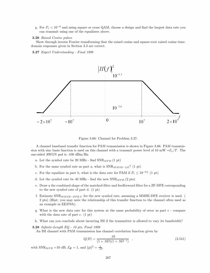
g. For Pe < 10−6 and using square or cross QAM, choose a design and find the largest data rate youcan transmit using one of the equalizers above.
3.26 Raised Cosine pulsesShow through inverse Fourier transforming that the raised cosine and square-root raised cosine time-
domain responses given in Section 3.3 are correct.
3.27 Expert Understanding - Final 1998
Figure 3.66: Channel for Problem 3.27.
A channel baseband transfer function for PAM transmission is shown in Figure 3.66. PAM transmis-sion with sinc basis function is used on this channel with a transmit power level of 10 mW =Ex/T . Theone-sided AWGN psd is -100 dBm/Hz.
a. Let the symbol rate be 20 MHz - find SNRMFB .(1 pt)
b. For the same symbol rate as part a, what is SNRMMSE−LE? (1 pt)
c. For the equalizer in part b, what is the data rate for PAM if Pe ≤ 10−6? (1 pt)
d. Let the symbol rate be 40 MHz - find the new SNRMFB .(2 pts)
e. Draw a the combined shape of the matched-filter and feedforward filter for a ZF-DFE correspondingto the new symbol rate of part d. (1 pt)
f. Estimate SNRMMSE−DFE,U for the new symbol rate, assuming a MMSE-DFE receiver is used. (2 pts) (Hint: you may note the relationship of this transfer function to the channel often used asan example in EE379A).
g. What is the new data rate for this system at the same probability of error as part c - comparewith the data rate of part c. (1 pt)
h. What can you conclude about incurring ISI if the transmitter is allowed to vary its bandwidth?
3.28 Infinite-Length EQ - 10 pts, Final 1998An ISI channel with PAM transmission has channel correlation function given by
Q(D) =.19
(1 + .9D)(1 + .9D−1), (3.541)
with SNRMFB =10 dB, Ex = 1, and ‖p‖2 = 1.19 .
267

a. (3 pts) Find WZFE(D), σ2ZFE , and SNRZFE .
b. (1 pt) Find WMMSE−LE(D)
c. (3 pts) Find WZF−DFE (D), BZF−DFE (D), and SNRZF−DFE .
d. (3 pts) Find WMMSE−DFE(D), BMMSE−DFE (D), and SNRMMSE−DFE,U .
3.29 Finite-Length EQ - 9 pts, Final 1998A baseband channel is given by
P (f) ={ √
T ·(1 − .7e2πfT
)|f | < .5
T0 |f | ≥ .5
T
(3.542)
and finite-length equalization is used with anti-alias perfect LPR with gain√
T followed by symbol-ratesampling. After the sampling, a maximum complexity of 3 taps TOTAL over a feedforward filter and afeedback filter can be tolerated. Ex = 2 and N0
2 = .01 for a symbol rate of 1/T = 100kHz is used withPAM transmission. Given the complexity constraint, find the highest data rate achievable with PAMtransmission when the corresponding probability of symbol error must be less than 10−5.
3.30 Equalizers - Miterm 2000 - 10 ptsPAM transmission on a filtered AWGN channel uses basic function ϕ(t) = 1√
T· sinc
(tT
)with T = 1
and undergoes channel impulse response with Fourier transform (|a| < 1)
H(ω) ={
11+a·eω |ω| ≤ π
0 |ω| > π(3.543)
and SNR = Exσ2 = 15 dB.
a. Find the Fourier Transform of the pulse response, P (ω)? (1 pt)
b. Find ‖p‖2. (2 pts)
c. Find Q(D), the function characterizing ISI. (3 pts)
d. Find the W (D) for the zero-forcing and MMSE linear equalizers on this channel. (3 pts)
e. If a = 0, what data rate is achievable on this channel according to the gap approximation atPe = 10−6? (1 pt)
3.31 Diversity Channel - Final 2000 - 6 ptsWe would like to evaluate the channel studied throughout this course and in the text with the same
input energy and noise PSD versus almost the same channel except that two receivers independentlyreceive:
• an undistorted delayed-by-T signal (that is P (D) = D), and
• a signal that is not delayed, but reduced to 90% of its amplitude (that is P (D) = .9).
a. Find Q(D), ‖p‖, and SNRMFB for the later diversity channel. (3 pts)
b. Find the performance of the MMSE-LE, MMSE-DFE for the later diversity channel and compareto that on the original one-receiver channel and with respect to the matched filter bound. (2 pts)
c. Find the probability of bit error on the diversity channel for the case of 1 bit/dimension transmis-sion. (1 pt)
3.32 Do we understand basic detection - Final 2000 - 9 ptsA filtered AWGN channel with T = 1 has pulse response p(t) = sinc(t)+sinc(t−1) with SNRMFB =
14.2 dB.
268
a. Find the probability of error for a ZF-DFE if a binary symbol is transmitted (2 pts).
b. The Tomlinson precoder in this special case of a monic pulse response with all unity coefficientscan be replaced by a simpler precoder whose output is
x′k =
{x′
k−1 if xk = 1−x′
k−1 if xk = −1 (3.544)
Find the possible channel outputs and determine an SBS decoder rule. What is the performance(probability of error) for this decoder? (2 pts)
c. Suppose this channel is used one time for the transmission of one of the 8 4-dimensional messagesthat are defined by [+ ± ± ±], which produce 8 possible 5-dimensional outputs. ML detectionis now used for this multidimensional 1-shot channel. What are the new minimum distance andnumber of nearest neighbors and how do they relate to those for the system in part a? What isthe new number of bits per output dimension? (3 pts)
d. Does the probability of error change significantly if the input is extended to arbitrarily long blocklength N with only the first sample fixed at +, and all other inputs being equally likely + or −?What happens to the number of bits per output dimension in this case? (2 pts).
3.33 Equalization - Final 2000 - 10 ptsPAM transmission is used on a filtered AWGN channel with N0
2 = .01, T = 1, and pulse repsonsep(t) = sinc(t) + 1.8sinc(t − 1) + .81sinc(t − 1). The desired probability of symbol error is 10−6.
a. Find ‖p‖2, SNRMFB, AND Q(D) for this channel. (2 pts)
b. Find the MMSE-LE and corresponding unbiased SNR for this channel. (2 pts)
c. Find the ZF-DFE detection SNR and loss with respect to SNRMFB . (1 pt)
d. Find the MMSE-DFE. Also compute the MMSE-DFE SNR and maximum data rate in bits/dimensionusing the gap approximation. (3 pts)
e. Draw the flexible (Laroia) precoder for the MMSE-DFE and draw the system from transmit symbolto detector in the receiver using this precoder. Implement this precoder for the largest number ofinteger bits that can be transmitted according to your answer in part (d). (2 pts)
3.34 Finite-Length Equalizer Design - Final 2000 - 15 ptsA filtered AWGN channel has impulse response h(t) = 1
T · 1
1+(
107t3
)2 and is used in the transmission
system of Figure 3.67. QAM transmission with 1/T = 1 MHz and carrier frequency fc = 600kHz areused on this channel. The AWGN psd is N0
2 = −86.5 dBm/Hz. The transmit power is ExT =1 mW. The
oversampling factor for the equalizer design is chosen as l = 2. Square-root raised cosine filtering with10% excess bandwidth is applied as a transmit filter, and an ideal filter is used for anti-alias filtering atthe receiver. A matlab subroutine at the course web site may be useful in computing responses in thefrequency domain.
a. Find ν so that an FIR pulse response approximates this pulse response so that less than 5% errorin ‖p‖2.
b. Calculate SNRMFB . Determine a reasonable set of parameters and settings for an FIR MMSE-LEand the corresponding data rate at Pe = 10−7. Calculate the data rate using both an integer anda possibly non-integer number of bits/symbol. (4 pts)
c. Repeat part b for an FIR MMSE-DFE design and draw receiver. Calculate the data rate usingboth an integer and a possibly non-integer number of bits/symbol. (3 pts)
269

Figure 3.67: Transmission system for Problem 3.34.
d. Can you find a way to improve the data rate on this channel by changing the symbol rate and orcarrier frequency? (2 pts)
3.35 Telephone-Line Transmission with “T1”Digital transmission on telephone lines necessarily must pass through two “isolation transformers” as
illustrated in Figure 3.68. These transformers prevent large D.C. voltages accidentally placed on the linefrom unintentionally harming the telephone line or equipment attached to it, and they provide immunityto earth currents, noises, and ground loops. These transformers also introduce ISI.
Figure 3.68: Illustration of a telephone-line data transmission for Problem 3.35.
a. The “derivative taking” combined characteristic of the transformers can be approximately modeledat a sampling rate of 1/T = 1.544 MHz as successive differences between channel input symbols.For sufficiently short transmission lines, the rest of the line can be modeled as distortionless. Whatis a reasonable partial-response model for the channel H(D)? Sketch the channel transfer function.Is there ISI?
b. How would a zero-forcing decision-feedback equalizer generally perform on this channel with respectto the case where channel output energy was the same but there are no transformers?
c. What are some of the drawbacks of a ZF-DFE on this channel?
d. Suppose a Tomlinson precoder were used on the channel with M = 2, how much is transmitenergy increased generally? Can you reduce this increase by good choice of initial condition forthe Tomlinson Precoder?
270

e. Show how a binary precoder and corresponding decoder can significantly simplify the implemen-tation of a detector. What is the loss with respect to optimum MFB performance on this channelwith your precoder and detector?
f. Suppose the channel were not exactly a PR channel as in part a, but were relatively close. Char-acterize the loss in performance that you would expect to see for your detector.
3.36 Magnetic Recording ChannelDigital magnetic information storage (i.e., disks) and retrieval makes use of the storage of magnetic
fluexes on a magnetic disk. The disk spins under a “read head” and by Maxwell’s laws the read-headwire senses flus changes in the moving magnetic field, thus generating a read current that is translatedinto a voltage through amplifiers succeeding the read head. Change in flux is often encoded to mean a“1” was stored and no change means a “0” was stored. The read head has finite band limitations also.
a. Pick a partial-resonse channel with ν = 2 that models the read-back channel. Sketch the magnitudecharacteristic (versus frequency) for your channel and justify its use.
b. How would a zero-forcing decision-feedback equalizer generally perform on this channel with respectto the best case where all read-head channel output energy convenyed either a positive or negativepolarity for each pulse?
c. What are some of the drawbacks of a ZF-DFE on this channel?
d. Suppose a Tomlinson precoder were used on the channel with M = 2, how much is transmitenergy increased generally? Can you reduce this increase by good choice of initial condition forthe Tomlinson Precoder?
e. Show how a binary precoder and corresponding decoder can significantly simplify the implemen-tation of a detector. What is the loss with respect to optimum MFB performance on this channelwith your precoder and detector?
f. Suppose the channel were not exactly a PR channel as in part a, but were relatively close. Char-acterize the loss in performance that you would expect to see for your detector.
g. Suppose the density (bits per linear inch) of a disk is to be increased so one can store more fileson it. What new partial response might apply with the same read-channel electronics, but with acorrespondingly faster symbol rate?
3.37 Tomlinson preocoding and simple precodingIn Section 3.8, the simple precoder for H(D) = 1 + D is derived.
a. Design the Tomlinson precoder corresponding to a ZF-DFE for this channel with the possiblebinary inputs to the precoder being ±1. (4 pts)
b. How many distinct outputs are produced by the Tomlinson Precoder assuming an initial state(feedback D element contents) of zero for the precoder. (1 pt)
c. Compute the average energy of the Tomlinson precoder output. (1 pt)
d. How many possible outputs are produced by the simple precoder with binary inputs? (1 pt)
e. Compute the average energy of the channel input for the simple precoder with the input constel-lation of part (a). (1 pt)
3.38 Flexible precoding and simple precodingIn Section 3.8, the simple precoder for H(D) = 1 + D is derived.
a. Design the Flexible precoder corresponding to a ZF-DFE for this channel with the possible binaryinputs to the precoder being ±1. (4 pts)
271

b. How many distinct outputs are produced by the Flexible Precoder assuming an initial state (feed-back D element contents) of zero for the precoder. (1 pt)
c. Compute the average energy of the Flexible precoder output. (1 pt)
d. How many possible outputs are produced by the simple precoder with binary inputs? (1 pt)
e. Compute the average energy of the channel input for the simple precoder with the input constel-lation of part (a). (1 pt)
3.39 Partial Response Precoding and the ZF-DFEConsider an AWGN with H(D) = (1 − D)2 with noise variance σ2 and one-dimensional real input
xk = ±1.
a. Determine a partial-response (PR) precoder for the channel, as well as the decoding rule for thenoiseless channel output. (2 pts)
b. What are the possible noiseless outputs and their probabilities? From these, determine the Pe forthe precoded channel. (4 pts)
c. If the partial-response precoder is used with symbol-by-symbol detection, what is the loss withrespect to the MFB? Ignore nearest neighbor terms for this calculation since the MFB concernsonly the argument of the Q-function. (1 pt)
d. If a ZF-DFE is used instead of a precoder for this channel, so that Pc(D) = 1− 2D + D2, what isη0? Determine also the SNR loss with respect to the SNRMFB (2 pts)
e. Compare this with the performance of the precoder, ignoring nearest neighbor calculations. (1 pt)
3.40 Error propagation and nearest neighborsConsider the H(D) = 1 − D2 channel with AWGN noise variance σ2 and d = 2 and 4-level PAM
transmission.
a. State the precoding rule and the noiseless decoding rule. (1 pts)
b. Find the possible noiseless outputs and their probabilities. Find also Ne and Pe with the use ofprecoding. (4 pts)
c. Suppose a ZF-DFE is used on this system and that at time k = 0 an incorrect decision x0− x0 = 2occurs. This incorrect decision affects zk at time k = 2. Find the Ne (taking the error at k = 0into account) for the ZF-DFE. From this, determine the Pe with the effect of error propagationincluded. (4 pts)
d. Compare the Pe in part (c) with that of the use of the precoder in part (a). (1 pt)
3.41 Forcing Partial ResponseConsider a H(D) = 1 + .9D channel with AWGN noise variance σ2. We would like to convert this
to a 1 + D channel
a. Design an equalizer that will convert the channel to a 1 + D channel. (2 pts)
b. The received signal is yk = xk + .9xk−1 + nk where nk is the AWGN. Find the autocorrelation ofthe noise after going through the receiver designed in part (a). Evaluate r0, r±1, and r±2. Is thenoise white? (3 pts)
c. Do you think that the noise terms would be more or less correlated if we were to convert a 1+ .1Dchannel to a 1 + D channel? You need only discuss briefly. (1 pt)
272

3.42 Final 2001 - Equalizers - 11 ptsPAM transmission on a filtered AWGN channel uses basis function ϕ(t) = 1√
Tsinc
(tT
)with T = 1
and undergoes channel impulse response with Fourier transform (|α| < 1)
H(ω) ={
11+a·eω |ω| ≤ π
0 |ω| > π(3.545)
and SNR = Exσ2 = 28 dB.
a. Find the Fourier Transform of the pulse response,P (ω) =? (1 pt)
b. Find ‖p‖2 . (1 pt)
c. Find Q(D), the function characterizing ISI. (2 pts)
d. Find the filters and sketch the block diagram of receiver for the MMSE-DFE on this channel fora = .9. (3 pts)
e. Estimate the data rate for uncoded PAM transmission and Pe < 10−6 that is achievable with youranswer in part d. (2 pts)
f. Draw a diagram of the better precoder’s (Tomlinson or Laroia), xmit and rcvr, implementationswith d = 2 in the transmitted constellation. (2 pts)
3.43 Final 2001 - Finite-Length Equalizer Design - 16 ptsTransmission lines can sometimes have their transfer function described by the function
H(f) = k · e−α·|f| (3.546)
where α and k are some positive real constants, here assigned the values α = 6π · 10−7 and k = 3π/10.Our task in this problem is to design a transmission system for such a transmission line. Initially webegin with 1/T = 800 kHz and carrier frequency fc = 600 kHz on this channel. The AWGN psd isN02
= −92 dBm/Hz. The transmit power is Ex/T = 1 mW. The oversampling factor for the equalizerdesign is chosen as l = 2. Square-root raised cosine filtering with 10% excess bandwidth is applied as atransmit filter and an ideal lowpass filter is used for anti-alias filtering at the receiver.
a. Find ν so that an FIR pulse response approximates this pulse response so that less than .25 dBerror in ‖p‖2 (that is, the norm square of the difference between the actual p(t) and the truncatedpk is less than (10.025 − 1) · ‖p‖2. (4 pts)
b. Determine a reasonable set of parameters and settings for an FIR MMSE-LE and the correspondingdata rate at Pe ≤ 10−7. Please print w filter coefficients. (2 pts)
c. Repeat part b for an FIR MMSE-DFE design and print coefficients. (2 pts)
d. Can you find a way to improve the data rate on this channel by changing the symbol rate and orcarrier frequency? Try to maximize the data rate with QAM transmission by a suitable choice ofcarrier frequency and symbol rate, and provide that data rate - you may maintain the assumptionof oversampling by a factor of 2 and 10% excess bandwidth. (6 pts)
e. Suppose a narrowband Gaussian noise with PSD -62 dBm/Hz were injected over a bandwith of1 kHz - hereustically, would you expect this to change the performance much? What would youexpect to happen in the filters of the DFE? ( 2 pts).
3.44 Final 2001 - Diversity Concept - 7 ptsAn additive white Gaussian noise channel supports QAM transmission with a symbol rate of 1/T =
100 kHz (with 0 % excess bandwidth) anywhere in a total baseband-equivalent bandwidth of 10 MHztransmission. Each 100 kHz wide QAM signal can be nominally received with an SNR of 14.5 dB withoutequalization. However, this 10 MHz wide channel has a 100 kHz wide band that is attenuated by 20dB with respect to the rest of the band, but the location of the frequency of this notch is not known inadvance to the designer. The transmitters are collocated.
273

a. What is the data rate sustainable at probability of bit error Pb ≤ 10−7 in the nominal condition?(1 pt)
b. What is the maximum number of simultaneous QAM users can share this channel at the perfor-mance level of part a if the notch does not exist? (1 pt)
c. What is the worst-case probability of error for the number of users in part b if the notch doesexist? (1 pt)
d. Suppose now (unlike part b) that the notch does exist, and the designer decides to send eachQAM signal in two distinct frequency bands. What is the worst-case probability of error for adiversity-equalization system applied to this channel? (1 pt)
e. For the same system as part c, what is the best SNR that a diversity equalizer system can achieve?(1 pt)
f. For the system of part c, how many users can now share the band all with probability of bit errorless than 10−7? Can you think of a way to improve this number closer to the level of the part b?(2 pts)
3.45 Final 2002 - Diversity Viewpoint - 12 ptsA time-varying wireless channel is used to send long packets of information that are decoded by a
receiver that uses a symbol-by-symbol decision device. The channel has pulse response in the familiarform:
P (ω) ={ √
T ·(1 + ai · e−ωT
)|ω| ≤ π
T0 |ω| > π
T
(3.547)
where ai may vary from packet to packet (but not within a packet). There is also AWGN with constantpower spectral density N0
2 = .1. QPSK (4QAM) is sent on this channel with symbol energy 2.
a. Find the best DFE SNR and corresponding probability of symbol error for the two cases whena1 = .9 and a2 = .5. (2 pts)
Now, suppose the transmitter can resend the same packet of symbols to the receiver, which candelay the channel output packet from the first transmission until the symbols from the new packetarrive. However, the same symbol-by-symbol detector is still to be used by the receiver.
b. Explain why this is a diversity situation. (1 pt)
c. Find a new SNRMFB for this situation. (1 pt)
d. Find the new function Q(D) for this diversity situation. (2 pts)
e. Determine the performance of the best DFE this time (SNR and Pe). ( 2 pts)
f. Compare the Pe of part e with the product of the two Pe’s found in part a. Comment. (2 pts)
g. Draw the receiver with RAKE illustrated as well as DFE, unbiasing, and decision device. (phasesplitter can be ignored in diagram and all quantities can be assumed complex.) (2 pts).
3.46 Precoder Diversity - Final 2003 - 7 ptsA system with 4PAM transmits over two discrete-time channels shown with the two independent
AWGN shown. (Ex = 1)
a. Find the RAKE matched filter(s) for this system ? (1 pt)
b. Find the single feedforward filter for a ZF-DFE? (1 pt)
c. Show the best precoder for the system created in part b. (1 pt)
274

Figure 3.69: Transmission system for Problem 3.47.
d. Find the SNR at the detector for this precoded system? (1 pt)
e. Find the loss in SNR with respect to the of either single channel. (1 pt)
f. Find the Pe for this precoded diversity system. (1 pt)
g. Find the probability that a packet of 1540 bytes contains one or more errors. (1 pt)
3.47 Equalizer Performance and MeansRecall that arithmetic mean, geometric mean, and harmonic mean are of the form 1
n
∑ni=1 xi,
(∏n
i=1 xi)1n ,(
1n
∑ni=1
1xi
)−1
, respectively. Furthermore, they satisfy the following inequalities:
1n
n∑
i=1
xi ≥
(n∏
i=1
xi
) 1n
≥
(1n
n∑
i=1
1xi
)−1
,
with equality when x1 = x2 = · · · = xn
a. (4 pts) Express SNRZFE , SNRZF−DFE , SNRMFB in terms of SNRMFB and frequency responseof the autocorrelation function qk. Prove that SNRZFE ≤ SNRZF−DFE ≤ SNRMFB using aboveinequalities. When does equality hold? hint : use
∫ b
a x(t)dt = limn→∞∑n
k=1 x( b−an k + a) · b−a
n
b. (4 pts) Similarly, prove that SNRMMSE−LE,U ≤ SNRMMSE−DFE,U ≤ SNRMFB using aboveinequalities. When does equality hold?
c. (4 pts) Compare SNRZF−DFE and SNRMMSE−LE. Can you say which scheme has betterperformance?
3.48 Unequal Channels (Moshe Malkin- instructor, Midterm 2007)Please assume the gap approximation works in all SNR ranges for this problem.
275

a. A sequence of 16-QAM symbols with in-phase component ak and quadrature component bk at timek is transmitted on a passband channel by the modulated signal
x(t) =√
2
{[∑
k
ak · φ(t − kT )
]· cos(ωct) −
[∑
k
bk · φ(t − kT )
]· sin(ωct)
}, (3.548)
where T = 40 ns, fc = 2.4 GHz, and the transmit power is 700 µW.
The waveform φ(t) is given by
φ(t) =1√T
sinc(
tT
)(3.549)
and the channel response is given by H(f) = e−j5πfT and so the received signal is given by
y(t) = h(t) ∗ x(t) + n(t) (3.550)
where n(t) is an additive white Gaussian noise random process with two-sided PSD of -100 dBm/Hz.
(i) (1 pts) What is the data rate for this system?
(ii) (2 pts) What are Ex, Ex and dmin for this constellation?
(iii) (1.5 pts) What is xbb(t)?
(iv) (1.5 pts) What is the ISI characterizing function q(t)? what is qk?
(v) (2 pts) What are Pe and Pe for an optimal ML detector?
(vi) (2 pts) Draw a block diagram of the receiver and label major components.
Unfortunately, the implementation of the baseband demodulator is faulty and the additiveGaussian noise power in the quadrature component is α = 4 times what it should be. Thatis, the noise variance of the quadrature component is αN0
2 = 2N0 while the noise variance inthe in-phase dimension is N0
2. Answer the following questions for this situation.
(vii) (2.5 pts) What is the receiver SNR?
(viii) (3 pts) What are Pe and Pe?
(ix) (1.5 pts) Instead of using QAM modulation as above, two independent 4-PAM constellations(with half the total energy allocated for each constellation) are now transmitted on the in-phase and quadrature channels, respectively. What is Pe averaged over both of the PAMconstellations?
(x) (3 pts) The transmitter realizes that if he allocates different energies for the in-phase andquadrature channels (BUT still using QAM modulation with an equal number ofbits for the in-phase and quadrature channels and original power constraint of 700µW ) he could improve the Pe performance from (aviii). What is the optimal energyallocation between the in-phase and quadrature channels? Given that we need Pe = 10−6,what is b and the achievable data rate?
(xi) (2.5 pts) Using the results from part (ax) find the minimal increase in transmit power neededto guarantee Pe = 10−6 for 16-QAM transmission?
The transmitter now decides to reduce losses. Given this increased noise in the quadra-ture dimension, the transmitter decides to use only the in-phase dimension for transmission(but subject to the original transmit power constraint of 700 µW ).
(xii) (1.5 pts) What data rate can be then supported that gives Pe = 10−6?
(xiii) (3 pts) Using a fair comparison, compare the QAM transmission system from part (ax) tothe single-dimensional scheme (N = 1) from part (axii). Which scheme is better?
276

(xiv) (3 pts) Can you derive a new transmission scheme that uses both the in-phase and quadraturechannels to get a higher data rate than part (ax)? (subject to the same Pe = 10−6 , andoriginal symbol rate and power constraint of 700 µW )
3.49 Equalizer Design (9 pts, Moshe Malkin- instructor, Final 2007)A transmission system uses the basis function φ(t) = sinc(t) with 1
T= 1 Hz. The Fourier transform
of the channel impulse response is:
H(f) ={ 1
1−0.5j·e−j2πf , for|f | ≤ 12
0, for|f | > 12 .
(3.551)
and SNR = εx
σ2 = 10dB.
a. (1 pt) Find ||p||2 and Q(D).
b. (1 pt) Find WZFE (D) and WMMSE−LE(D).
c. (1 pt) Find W (D) and B(D) for ZF-DFE.
d. (2 pts) Find W (D) and B(D) for MMSE-DFE (Hint: the roots of the numerator of Q(D) +1/SNRMFB are 22.4555j and 0.0445j).
e. (0.5 pts) What is SNRZF−DFE?
f. (1.5 pts) Design a Tomlinson-Harashima precoder based on the ZF-DFE. Show both the precoderand the corresponding receiver (For any M).
g. (2 pts) Design a Laroia precoder based on the ZF-DFE. Assume you are using 4-QAM modulation.Show both the precoder and the corresponding receiver. Make sure to mention which kind ofconstellation is used at each SBS detector in your drawing.
3.50 Diversity (7 pts Moshe Malkin- instructor, Final 2007)A receiver has access to an infinite number of diversity channels where the output of channel i at
time k is
yk,i = xk + 0.9 · xk+1 + nk,i, i = 0, 1, 2, . . .
where nk,i is a Gaussian noise process independent across time and across all the channels, and withvariance σ2
i = 1.2i · 0.181. Also, Ex = 1.
a. (1 pts) Find SNRMFB,i, the SNRMFB for channel i.
b. (2 pts) What is the matched filter for each diversity channel?
c. (1.5 pts) What is the resulting Q(D) for this diversity system?
d. (2.5 pts) What is the detector SNR for this system for a ZF-DFE receiver?
3.51 DFE with Finite Length Feedback Filter (9 pts Moshe Malkin- instructor, Final 2007)A symbol-rate sampled MMSE-DFE structure, where the received signal is filtered by a continuous
time matched filter, uses an infinite length feedforward filter. However, the MMSE-DFE feedback filterto be of finite length Nb.
a. (2 pts) Formulate the optimization problem you would have to solve to find the optimal feedfor-ward and feedback coefficients to minimize the mean squared error (Hint: Don’t approach this asa finite-length equalization problem as in section 3.7).
Assume that N02 = .181, Ex = 1, and P (D) = 1 + .9 · D−1. (and SNRMFB = 10 dB).
277

b. (2 pts) Using only 1 feedback tap (Nb = 1), determine the optimal feedforward and feedback filters(Hint: This is easy - you have already seen the solution before).
c. (2 pts) Now consider the ZF-DFE version of this problem. State the optimization problem for thissituation (analogous to part a).
Now, assume that we have P (D) = 11+0.9D−1 (and ‖p‖2 = 1
1−0.92 = 10.19
).
d. (3 pts) Determine the optimal feedforward and feedback filters for the ZF-DFE formulation usingonly 1 feedback tap (Nb = 1).
3.52 Packet Processing (10 pts Moshe Malkin- instructor, Final 2007)Suppose that in a packet-based transmission system, a receiver makes a decision from the set of
transmit symbols x1, x2, x3 based on the channel outputs y1, y2, y3, where
y3
y2
y1
=
p11 p12 p13
0 p22 p23
0 0 p33
x3
x2
x1
+
n3
n2
n1
=
0.6 1.9 −3.860 1.8 3.30 0 1.2
x3
x2
x1
+
n3
n2
n1
(3.552)
and where the noise autocorrelation matrix is given by
Rn = E
n3
n2
n1
[ n∗
3 n∗2 n∗
1
] =
0.3 0 00 0.5 00 0 0.1
. (3.553)
The inverse of the channel matrix is given by
0.6 1.9 −3.860 1.8 3.30 0 1.2
−1
=
1.67 −1.76 10.190 0.56 −1.520 0 0.83
. (3.554)
The transmit symbols are i.i.d with E§∞ = E§∈ = E§3 = ∈′.
a. (1.5 pts) What is the 3-tap zero-forcing equalizer for x1 based on the observation y1, y2, y3? Repeatfor x2 and x3.
b. (1 pts) What is the matrix ZFE for detecting x1, x2, and x3? (Hint: This is easy - all the workoccurred in the previous part)
c. (1.5 pts) What is the detection SNR for x1 using a ZFE? Answer the same for x2 and x3.
d. (1 pts) An engineer now realizes that the performance could be improved through use previousdecisions when detecting the current symbol. If the receiver starts by detecting x1, then x2, andfinally x3, describe how this modified ZF detector would work?
e. (1.5 pts) Assuming previous decisions are correct, what is now the detection SNR for each symbol?
f. (1 pts) The approach above does not necessarily minimize the MMSE. How would a packet MMSE-DFE work? How would you describe the feedback structure? (Don’t solve for the optimal matrices- just describe the signal processing that would take place).
g. (1 pts) Can the THP also be implemented for this packet based system? Describe how this wouldbe done (again, don’t solve - just describe how this would work).
278

Appendix A
Useful Results in Linear MinimumMean-Square Estimation
This appendix derives and/or lists some key results from linear Minimum Mean-Square-Error estimation.A linear MMSE estimate of some random variable x, given observations of some other random
sequences {yk}, chooses a set of parameters wk (with the index k having one distinct value for eachobservation of yk that is used) to minimize
E[|e|2]
(A.1)
where
e∆= x −
N−1∑
k=0
wk · yk . (A.2)
One can let N → ∞ without difficulty. The term linear MMSE estimate is derived from the linearcombination of the random variables yk in (A.2). More generally, it can be shown that the MMSEestimate is E [x/{yk}], the conditional expectation of x, given y0, ..., yN−1. which will be linear forjointly Gaussian x and {yk}. This text is interested only in linear MMSE estimates. In this text’sdevelopments, yi will usually be successive samples of some channel output sequence, and x will be thecurrent channel-input symbol that the receiver attempts to estimate.
A.1 The Orthogonality Principle
While (A.1) can be minimized directly by differentiation in each case or problem of interest, it is oftenfar more convenient to use a well-known principle of linear MMSE estimates - that is that the errorsignal e must always be uncorrelated with all the observed random variables in order for the MSE to beminimized.
Theorem A.1.1 (Orthogonality Principle) The MSE is minimized if and only if thefollowing condition is met
E [e · y∗k] = 0 ∀ k = 0, ..., N − 1 (A.3)
Proof: By writing |e|2 = [<(e)]2 + [=(e)]2, we may differentiate the MSE with respect toboth the real and imaginary parts of wk for each k of interest. The pertinent parts of the realand imaginary errors are (realizing that all other wi, i 6= k, will drop from the correspondingderivatives)
er = xr − wr,k · yr,k + wi,k · yi,k (A.4)ei = xi − wi,k · yr,k − wr,k · yi,k , (A.5)
279
where subscripts of r and i denote real and imaginary part in the obvious manner. Then, tooptimize over wr,k and wi,k,
∂|e|2
∂wr,k= 2er
∂er
∂wr,k+ 2ei
∂ei
∂wr,k= −2 (eryr,k + eiyi,k) = 0 (A.6)
∂|e|2
∂wi,k= 2er
∂er
∂wi,k+ 2ei
∂ei
∂wi,k= 2 (eryi,k − eiyr,k) = 0 . (A.7)
The desired result is found by taking expectations and rewriting the series of results abovein vector form. Since the MSE is positive-semi-definite quadratic in the parameters wr,k andwi,k, this setting must be a global minimum. If the MSE is strictly positive-definite, thenthis minimum is unique. QED.
A.2 Spectral Factorization
This section uses D-transform notation for sequences:
Definition A.2.1 (D- Transforms) A sequence {xk} has D-Transform X(D) =∑
k xkDk.
In this chapter, all sequences can be complex. The sequence {x∗−k} has a D-Transform X∗(D−∗) ∆=∑
k x∗kD−k.
Definition A.2.2 (Autocorrelation and Power Spectrum) If {xk} is any stationarycomplex sequence, its autocorrelation function is defined as the sequence Rxx(D) whoseterms are rxx,j = E[xkx
∗k−j]; symbolically1
Rxx(D) ∆= E[X(D) · X∗(D−∗)
]. (A.8)
By stationarity, rxx,j = r∗xx,−j and Rxx(D) = R∗xx(D−∗). The power spectrum of a
stationary sequence is the Fourier transform of its autocorrelation function, which is writtenas
Rxx(e−ωT ) = Rxx(D)|D=e−ωT , − π
T< ω ≤ π
T, (A.9)
which is real and nonnegative for all ω. Conversely, we say that any complex sequence R(D)for which R(D) = R∗(D−∗) is an autocorrelation function, and any function R(e−ωT ) thatis real and nonnegative over the interval {− π
T< ω ≤ π
T} is a power spectrum.
The quantity E[|xk|2
]is Ex, or Ex per dimension, and is determined by either the autocorrelation
function or the power spectrum as follows:
Ex = E[|xk|2
]= rxx,0 =
T
2π
∫ πT
− πT
R(e−ωT )dω . (A.10)
The spectral factorization of an autocorrelation function is:
Definition A.2.3 (Factorizability) An autocorrelation function R(D) will be called fac-torizable if it can be written in the form
R(D) = S0 · F (D) · F ∗(D−∗), (A.11)
where S0 is a positive real number and F (D) is a canonical filter response. A filter responseF (D) is called canonical if it is causal (fk = 0 for k < 0), monic (f0 = 1), and minimum-phase (all of its poles are outside the unit circle, and all of its zeroes are on or outside theunit circle). If F (D) is canonical, then F ∗(D−∗) is anticanonical; i.e., anticausal, monic,and maximum-phase.
1The expression Rxx(D)∆= E
[X(D)X∗(D−1)
]is used in a symbolic sense, since the terms of X(D)X∗(D−1) are of
the form∑
kxkx∗
k−j , implying the additional operation limN→∞[1/(2N + 1)]∑
−N≤k≤Non the sum in such terms.
280

If F (D) is a canonical response, then ‖f‖2 ∆=∑
j |fj|2 ≥ 1, with equality if and only if F (D) = 1,since F (D) is monic. This simple inequality has many uses, see Exercises for Chapter 3.
The following lemma from discrete-time spectral factorization theory describes when an autocorre-lation function is factorizable, and also gives the value of S0.
Lemma A.2.1 (Spectral Factorization) If R(e−ωT ) is any power spectrum such thatboth R(e−ωT ) and logR(e−ωT ) are integrable over − π
T< ω ≤ π
T, and R(D) is the corre-
sponding autocorrelation function, then there is a canonical discrete-time response F (D) thatsatisfies the equation
R(D) = S0 · F (D) · F ∗(D−∗), (A.12)
where the finite constant S0 is given by
logS0 =12π
∫ πT
− πT
log R(e−ωT )dω (A.13)
(where the logarithms can have any common base). For S0 to be finite, R(e−ωT ) satisfiesthe discrete-time Paley-Wiener criterion
12π
∫ πT
− πT
| logR(e−ωT )|dω < ∞ . (A.14)
Linear Prediction
The inverse of R(D) is also an autocorrelation function and can be factored when R(D) also satisfiesthe PW criterion with finite γ0. In this case, as with the MMSE-DFE in Section 3.6, the inverseautocorrelation factors as
R−1xx (D) = γ0 · G(D) · G∗(D−∗) . (A.15)
If x(D) is a discrete-time sequence with factorizable inverse autocorrelation function R−1xx (D) =
γ0G(D)G∗(D−∗), and A(D) is any causal and monic sequence, then 1−A(D) is a strictly causal sequencethat may be used as a prediction filter, and the prediction error sequence E(D) is given by
E(D) = X(D) − X(D)[1 − A(D)] = X(D)A(D) . (A.16)
The autocorrelation function of the prediction error sequence is
Ree(D) = Rxx(D) · A(D) · A∗(D−∗) =A(D) ·A∗(D−∗)
γ0 · G(D) ·G∗(D−∗), (A.17)
so its average energy satisfies Ee = S0‖1/g ∗ a‖2 ≥ S0 (since A(D)/G(D) is monic), with equality if andonly if A(D) is chosen as the whitening filter A(D) = G(D). The process X(D) ·G(D) is often calledthe innovations of the process X(D), which has mean square value S0 = 1/γ0. Thus, S0 of the directspectral factorization is the mean-square value of the innovations process or equivalent of the MMSEin linear prediction. X(D) can be viewed as being generated by inputting a white innovations processU (D) = G(D)X(D) with mean square value S0 into a filter F (D) so that X(D) = F (D)U (D).
The factorization of the inverse and resultant interpretation of the factor G(D) as a linear-predictionfilter helps develop an interest interpretation of the MMSE-DFE in Section 3.6.
A.2.1 Cholesky Factorization
Cholesky factorization is the finite-length equivalent of spectral factorization. In this finite-length case,there are really two factorizations, both of which converge to the infinite-length spectral factorization.
281

Cholesky Form 1 - Forward Prediction
Cholesky factorization of a positive semidefinite N × N matrix RN produces a unique upper triangularmonic (ones along the diagonal) matrix F N and a unique diagonal positive-semidefinite matrix SN suchthat
RN = F N SNF ∗N . (A.18)
It is convenient in transmission theory to think of the matrix RN as an autocorrelation matrix for Nsamples of some random vector process xk with ordering
XN =
xN−1
...x0
. (A.19)
A corresponding order of F N and SN is then
F N =
fN−1
fN−2...
f0
and SN =
sN−1 0 ... 00 sN−2 ... 0
0...
. . . 00 0 ... s0
. (A.20)
Since F N is monic, it is convenient to write
f i =[1 f i
]. (A.21)
The determinant of RN is easily found as
γ20 = |RN | =
N−1∏
n=0
sn . (A.22)
(or lnγ20 = ln |RN | for readers taking limits as N → ∞). A convenient description of RN ’s components
is then
RN =[
rN r∗1
r1 RN−1
]. (A.23)
The submatrix RN−1 has Cholesky Decomposition
RN−1 = F N−1SN−1F N−1 , (A.24)
which because of the 0 entries in the triangular and diagonal matrices shows the recursion inherent inCholesky decomposition (that is the F N−1 matrix is the lower right (N − 1) × (N − 1) submatrix ofF N , which is also upper triangular). The inverse of RN (pseudoinverse when singular) has a Choleskyfactorization
R−1N = G∗
N S−1N GN (A.25)
where F N = G−1N is also upper triangular and monic with ordering
GN =
gN−1
gN−2...
g0
. (A.26)
Also,gi = [1 gi] . (A.27)
282
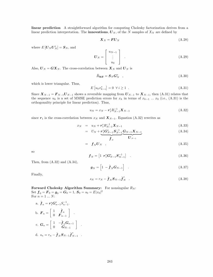
linear prediction A straightforward algorithm for computing Cholesky factorization derives from alinear prediction interpretation. The innovations, UN , of the N samples of XN are defined by
XN = FUN (A.28)
where E [UN U∗N ] = SN , and
UN =
uN−1
...u0
. (A.29)
Also, UN = GXN . The cross-correlation between XN and UN is
Rux = SN G∗N , (A.30)
which is lower triangular. Thus,E[ukx∗
k−i
]= 0 ∀ i ≥ 1 . (A.31)
Since XN−1 = F N−1UN−1 shows a reversible mapping from UN−1 to XN−1, then (A.31) relates thatthe sequence uk is a set of MMSE prediction errors for xk in terms of xk−1 ... x0 (i.e., (A.31) is theorthogonality principle for linear prediction). Thus,
uN = xN − r∗1R
−1N−1XN−1 (A.32)
since r1 is the cross-correlation between xN and XN−1. Equation (A.32) rewrites as
xN = uN + r∗1R
−1N−1XN−1 (A.33)
= UN + r∗1G
∗N−1S
−1N−1︸ ︷︷ ︸
˜fN
GN−1XN−1︸ ︷︷ ︸UN−1
(A.34)
= fNUN , (A.35)
sofN =
[1 r∗
1G∗N−1S
−1N−1
]. (A.36)
Then, from (A.32) and (A.34),gN =
[1 − fNGN−1
]. (A.37)
Finally,sN = rN − fN SN−1f
∗N . (A.38)
Forward Cholesky Algorithm Summary: For nonsingular RN :Set f0 = F 0 = g0 = G0 = 1, S0 = s0 = E|x0|2For n = 1 ... N :
a. fn = r∗1G
∗n−1S
−1n−1.
b. F n =[
1 fn
0 F n−1
].
c. Gn =[
1 −fnGn−1
0 GN−1
].
d. sn = rn − fN SN−1f∗N−1 .
283
A singular RN means that sn = 0 for at least one index n = i, which is equivalent to ui = 0, meaningthat xi can be exactly predicted from the samples xi−1 ... x0 or equivalently can be exactly constructedfrom ui−1 ... u0. In this case, Cholesky factorization is not unique. One factorization is to save F i and Gi
and “restart” the algorithm for n > i realizing that xi is equivalent to knowing all lower-index samples.The new F n>i and Gn>i created will have smaller dimension, but when the algorithm is complete, zeroscan be added to all the “right-most” positions of F and G, and maintaining the previous F i and Gi forthe lower rightmost positions.
That is,
F N =[
F n>i 00 F i
]and GN =
[Gn>i 0
0 Gi
](A.39)
and
SN =
Sn>i 0 00 0 00 0 Si−1
. (A.40)
The forward Cholesky factorization can also be written
RN = G−1N SNG−∗
N , (A.41)
which is convenient for the alternative finite-length MMSE-DFE interpretations in Section 3.7.
Cholesky Form 2 - Backward Prediction
The backward Cholesky factorization is into a lower-diagonal-upper (instead of the upper-diagonal-lowerin forward prediction). This involves extension of RN on the lower right corner instead of at the upper-left corner. Rather than repeat the development of forward prediction, this section notes that the reversebackward prediction problem is inherent in the algorithm already given, except that this algorithm isperformed on the inverse (which, granted, might be harder to compute than just repeating the stepsabove with the appropriate transpositions).
The inverse matrix QN = R−1N = G∗
N S−1N GN is also an autocorrelation matrix for some process
Y N with innovations V N where Y N = G∗NV N such that E [V N V ∗
N ] = S−1N . If Q is singular, then its
pseudoinverse is used by definition here. Thus,
V N = F ∗NY , (A.42)
illustrating the backward prediction error v1−N = f∗NY N−1 where f
∗N is the N th row of F ∗
N or equiva-lently fN is the last column of F N .
This factorization of Q is lower-diagonal-upper and the filters fn are backward prediction filters fory1−n in terms of y2−n ... y0. So to perform backward-prediction Cholesky, first invert the given Qautocorrelation matrix to get R and then do forward Cholesky on the inverse (RN = F NSN F ∗
N =G−1
N SG−∗N . Then, the backward Cholesky factorization uses the G of forward Cholesky (for R = Q−1)
inQ = G∗
NS−1N GN . (A.43)
Infinite-length convergence
For infinite-length stationary sequences, one takes the limit as N → ∞ in either forward or backwardCholesky factorization. In this case, the matrix R (and therefore Q) must be nonsingular to satsifythe Paley-Weiner Criterion. The equivalence to spectral factorization is evident from the two linear-prediction interpretations for finite-length and infinite length series of samples from random processes.
For the stationary case, the concepts of forward and backward prediction are the same so that theforward predictor is just the time reverse of the coefficents in the backward predictor.
Thus, the inverse autocorrelation function factors as
R−1(D) = γ0G(D)G∗(D−∗) , (A.44)
284

where G(D) is the forward prediction polynomial (and its time reverse specified by G∗(D−∗) is thebackward prediction polynomial). The series of matrices {Rn}n=1:∞ formed from the coefficients ofR(D) creates a series of linear predictors {gn}n=1:∞ with D-transforms Gn(D). In the limit as N → ∞for a stationary nonsingular series,
limn→∞
Gn(D) = G(D) . (A.45)
Similarly,lim
n→∞G∗
n(D) = G∗(D−∗) . (A.46)
As N → ∞, the prediction error varianc,es SN−1, should tend to a constant. Finally, defining thegeometric-average determinants as S0,n = |R|1/N and γ0,N = |R−1|1/N
limn→∞
S0,n = S0 = e
{T2π
∫ π/T
−π/Tln(R(e−ωT ))dω
}(A.47)
limn→∞
γ0,n(D) = γ0 = e−{
T2π
∫ π/T
−π/Tln(R(e−ωT ))dω
}. (A.48)
The convergence to these limits implies that the series of filters converges or that the bottom row (lastcolumn) of the Cholesky factors tends to a constant repeated row.
Interestingly, a Cholesky factorization of a singular process exists only for finite lengths. Using themodifications to Cholesky factorization suggested above with “restarting,” it becomes obvious why sucha process cannot converge to a constant limit and so only nonsingular processes are considered in spectralfactorization. Factorization of a singular process at infinite-length involves separating that process intoa sum of subprocesses, each of which is resampled at a new sampling rate so that the PW criterion(nonsingular needs PW) is satisfied over each of the subbands associated with these processes. This isequivalent to the “restarting” of Cholesky at infinite length. For more, see Chapter 5.
285

Appendix B
Equalization for Partial Response
Just as practical channels are often not free of intersymbol interference, such channels are rarely equalto some desirable partial-response (or even controlled-ISI) polynomial. Thus, an equalizer may be usedto adjust the channel’s shape to that of the desired partial-response polynomial. This equalizer thenenables the use of a partial-response sequence detector or a symbol-by-symbol detector at its output(with partial-response precoder). The performance of either of these types of detectors is particularlysensitive to errors in estimating the channel, and so the equalizer can be crucial to achieving the highestlevels of performance in the partial-response communication channel. There are a variety of ways inwhich equalization can be used in conjunction with either sequence detection and/or symbol-by-symboldetection. This section introduces some equalization methods for partial-response signaling.
Chapter 9 studies sequence detection so terms related to it like MLSD (maximum likelihood sequencedetection) and Viterbi detectors/algorithm are pertinent to readers already familiar with Chapter 9contents and can be ignored by other readers otherwise in this Appendix.
B.1 Controlled ISI with the DFE
Section 3.8.2 showed that a minimum-phase channel polynomial H(D) can be derived from the feedbacksection of a DFE. This polynomial is often a good controlled intersymbol interference model of thechannel when H(D) has finite degree ν. When H(D) is of larger degree or infinite degree, the first νcoefficients of H(D) form a controlled intersymbol interference channel. Thus, sequence detection onthe output of the feedforward filter of a DFE can be designed using the controlled ISI polynomial H(D)or approximations to it.
B.1.1 ZF-DFE and the Optimum Sequence Detector
Section 3.1 showed that the sampled outputs, yk, of the receiver matched filter form a sufficient statisticfor the underlying symbol sequence. Thus a maximum likelihood (or MAP) detector can be designedthat uses the sequence yk to estimate the input symbol sequence xk without performance loss. Thefeedforward filter 1/(η0‖p‖H∗(D−∗)) of the ZF-DFE is invertible when Q(D) is factorizable. The re-versibility theorem of Chapter 1 then states that a maximum likelihood detector that observes the outputof this invertible ZF-DFE-feedforward filter to estimate xk also has no performance loss with respect tooptimum. The feedforward filter output has D-transform
Z(D) = X(D)H(D) + N ′(D) . (B.1)
The noise sequence n′k is exactly white Gaussian for the ZF-DFE, so the ZF-DFE produces an equivalent
channel H(D). If H(D) is of finite degree ν, then a sequence detector can be designed based on thecontrolled-ISI polynomial H(D) and this detector has minimum probability of error. Figure B.1 showssuch an optimum receiver. When H(D) has larger degree than some desired ν determined by complexityconstraints, then the first ν feedback taps of H(D) determine
H ′(D) = 1 + h1D1 + ... + hνDν , (B.2)
286

Figure B.1: The optimum maximum-likelihood detector, implemented with the assistance of the WMF,the feedforward section of the ZF-DFE
Figure B.2: Limiting the number of states with ZF-DFE and MLSD.
a controlled-ISI channel. Figure B.2 illustrates the use of the ZF-DFE and a sequence detector. Thesecond feedback section contains all the channel coefficients that are not used by the sequence detector.These coefficients have delay greater than ν. When this second feedback section has zero coefficients, thenthe configuration shown in Figure B.2 is an optimum detector. When the additional feedback sectionis not zero, then this structure is intermediate in performance between optimum and the ZF-DFE withsymbol-by-symbol detection. The inside feedback section is replaced by a modulo symbol-by-symboldetector when precoding is used.
Increase of ν causes the minimum distance to increase, or at worst, remain the same (which is provedsimply by examining a trellis with more states and realizing that the smaller degree H ′(D) is a sub trellisfor which distance cannot be greater. Thus, the ZF-DFE with sequence detector in Figure B.2 definesa series of increasingly complex receivers whose performance approach optimum as ν → ∞. A propertyof a minimum-phase H(D) is that
ν′∑
i=0
|hi|2 = ‖h′‖2 (B.3)
is maximum for all ν′ ≥ 0. No other polynomial (that also preserves the AWGN at the feedforward filteroutput) can have greater energy. Thus the SNR of the signal entering the Viterbi Detector in FigureB.2, Ex‖h′‖2
N02
, also increases (nondecreasing) with ν. This SNR must be less than or equal to SNRMFB.
287

Figure B.3: Partial-response linear equalization.
B.1.2 MMSE-DFE and sequence detection
Symbol-by-symbol detection’s objective is to maximize SNR in an unbiased detector, and so SNR max-imization was applied in Chapter 3 to the DFE to obtain the MMSE-DFE. A bias in symbol-by-symboldetector was removed to minimize probability of error. The monic, causal, minimum-phase, and unbi-ased feedback polynomial was denoted GU (D) in Section 3.6. A sequence detector can use the samestructures as shown in Figure B.1 and B.2 with H(D) replaced by Gu(D). For instance, Figure B.4 isthe same as Figure B.2, with an unbiased MMSE-DFE’s MS-WMF replacing the WMF of the ZF-DFE.A truncated version of GU(D) corresponding to H ′(D) is denoted G′
U(D). The error sequence asso-ciated with the unbiased MMSE-DFE is not quite white, nor is it Gaussian. So, a sequence detectorbased on squared distance is not quite optimum, but it is nevertheless commonly used because the exactoptimum detector could be much more complex. As ν increases, the probability of error decreases fromthe level of the unbiased MMSE-DFE, SNRMMSE−DFE,U when ν = 0, to that of the optimum detectorwhen ν → ∞. The matched filter bound, as always, remains unchanged and is not necessarily obtained.However, minimum distance does increase with ν in the sequence detectors based on a increasing-degreeseries of GU(D).
B.2 Equalization with Fixed Partial Response B(D)
The derivations of Section 3.6 on the MMSE-DFE included the case where B(D) 6= G′(D), which thissection reuses.
B.2.1 The Partial Response Linear Equalization Case
In the linear equalizer case, the equalization error sequence becomes
Epr(D) = B(D)X(D) − W (D)Y (D) . (B.4)
Section 3.6 minimized MSE for any B(D) over the coefficients in W (D). The solution was found bysetting E
[Epr(D)y∗(D−1)
]= 0, to obtain
W (D) = B(D)Rxy(D)Ryy(D)
=B(D)
‖p‖ (Q(D) + 1/SNRMFB), (B.5)
which is just the MMSE-LE cascaded with B(D). Figure B.3, shows the MMSE-PREQ (MMSE -“Partial Response Equalizer”). The designer need only realize the MMSE-LE of Section 3.4 and followit by a filter of the desired partial-response (or controlled-ISI) polynomial B(D).1 For this choice ofW (D), the error sequence is
Epr(D) = B(D)X(D) − B(D)Z(D) = B(D) [E(D)] (B.6)1This also follows from the linearity of the MMSE estimator.
288

where E(D) is the error sequence associated with the MMSE-LE. From (B.6),
Repr,epr (D) = B(D)Ree(D)B∗(D−1) =B(D)N0
2 B∗(D−1)‖p‖2 (Q(D) + 1/SNRMFB)
. (B.7)
Thus, the MMSE for the PREQ can be computed as
σ2MMSE-PREQ =
T
2π
∫ πT
− πT
|B(e−ωT )|2N02
‖p‖2 (Q(e−ωT ) + 1/SNRMFB)dω . (B.8)
The symbol-by-symbol detector is equivalent to subtracting (B(D) − 1)X(D) before detection based ondecision regions determined by xk. The SNRMMSE-PREQ becomes
SNRMMSE-PREQ =Ex
σ2MMSE-PREQ
. (B.9)
This performance can be better or worse than the MMSE-LE, depending on the choice of B(D); thedesigner usually selects B(D) so that SNRMMSE-PREQ > SNRMMSE−LE. This receiver also has abias, but it is usually ignored because of the integer coefficients in B(D) – any bias removal could causethe coefficients to be noninteger.
While the MMSE-PREQ should be used for the case where symbol-by-symbol and precoding arebeing used, the error sequence Epr = B(D)E(D) is not a white noise sequence (nor is E(D) for theMMSE-LE), so that a Viterbi Detector designed for AWGN on the channel B(D) would not be theoptimum detector for our MMSE-PREQ (with scaling to remove bias). In this case, the ZF-PREQ,obtained by setting SNRMFB → ∞ in the above formulae, would also not have a white error sequence.Thus a linear equalizer for a partial response channel B(D) that is followed by a Viterbi Detectordesigned for AWGN may not be very close to an optimum detection combination, unless the channelpulse response were already very close to B(D), so that equalization was not initially necessary. Whilethis is a seemingly simple observation made here, there are a number of systems proposed for use indisk-storage detection that overlook this basic observation, and do equalize to partial response, “color”the noise spectrum, and then use a WGN Viterbi Detector. The means by which to correct this situationis the PR-DFE of the next subsection.
B.2.2 The Partial-Response Decision Feedback Equalizer
If B(D) 6= G(D) and the design of the detector mandates a partial-response channel with polynomialB(D), then the optimal MMSE-PRDFE is shown in Figure B.4.
Again, using our earlier result that for any feedback section GU (D) = B(D) + B(D). The errorsequence is the same as that for the MMSE-DFE, and is therefore a white sequence. The signal betweenthe the two feedback sections in Figure B.4 is input to the sequence or symbol-by-symbol detector. Thissignal can be processed on a symbol-by-symbol basis if precoding is used (and also scaling is used toremove the bias - the scaling is again the same scaling as used in the MMSE-DFE), and BU (D) =GU(D) − BU (D), where
BU (D) =SNRMMSE−DFE
SNRMMSE−DFE,U
[B(D) − 1
SNRMMSE−DFE
]. (B.10)
However, since the MMSE-PRDFE error sequence is white, and because the bias is usually small so thatthe error sequence in the unbiased case is also almost white, the designer can reasonably use a ViterbiDetector designed for B(D) with white noise.
If the bias is not negligible, then a ZF-PRDFE should be used, which is illustrated in Figure B.2,and the filter settings are obtained by setting SNRMFB → ∞ in the above formula.
289

Figure B.4: Partial-response DFE with B(D)
290

Appendix C
The Matrix Inversion Lemma:
The matrix inversion lemma:
[A + BCD]−1 = A−1 − A−1B[C−1 + DA−1B
]−1DA−1 . (C.1)
291


![1 The Performance of Successive Interference …arXiv:1402.1557v1 [cs.IT] 7 Feb 2014 1 The Performance of Successive Interference Cancellation in Random Wireless Networks Xinchen Zhang](https://img.dokumen.tips/doc/110x75/5eaef451297d84714111d095/1-the-performance-of-successive-interference-arxiv14021557v1-csit-7-feb-2014.jpg)