Loudspeaker Response Optimization with the aid of … · Loudspeaker Response Optimization with the aid of ... such a stimulus is not as practical due to several limitations [1

Loudspeaker Response Optimization with the aid of Impulse Response

R. Balistreri

Klipsch Group, Inc., Indianapolis, IN, USA

Abstract: COMSOL Multiphysics® simulation software is receiving a lot of attention in the loudspeaker industry

thanks to the quality of the results it provides making it an essential tool to optimize geometries so that the best

reproduction capabilities of the loudspeaker system are achieved.

Setting up a loudspeaker simulation requires defining a geometry with moving diaphragm. This can be done simply

by specifying diaphragm’s velocity within the Acoustics Module; or by including full definitions of the

Electromagnetic domain, Mechanical domain and Acoustical domain in a Multiphysics setup. Alternatively, it can be

done with just the AC/DC and Acoustics Modules with the aid of lumped circuit equivalents. Whatever the case, the

analysis is typically done in the frequency domain on a series of values for frequencies in order to profile a resulting

frequency response. This process of iterations is rather time consuming for an average workstation.

With the latest 5.3 update, improvements were done in the Acoustics Module on time domain that allow for an easier

setup of acoustic simulations. It is now practical to use of an impulse response analysis in time domain. Results with

a Fourier Transform can give an idea of the behavior in the frequency response for a quick optimization. A more

detailed inspection in frequency domain is possible by mapping results from time domain so that the far field can be

calculated. Additional analysis time is saved by focusing only on frequencies of interest within the same model which,

when thinking of iterative changes, speeds up optimization of the geometries for the intended design target. This

paper illustrates such an approach to loudspeaker design.

Introduction

In acoustic measurements, it has been extensively

proved essential the use of the impulse response

formulation in determining the frequency response of

a loudspeakers.

For acoustic room measurements, examples of a good

approximation of an acoustic impulse might be the

popping of a balloon or the firing of a blank. A

complete time domain recording of the impulse,

including its decay, provides most of the information

necessary for that study.

For the measurements of electrical transducer systems

such a stimulus is not as practical due to several

limitations [1]. The first limitation is the high crest

factor as loudspeakers could be driven out of their

linearity range. An additional limitation is poor signal

to noise ratio because all the energy is emitted in a

brief fraction of time. Measuring with Chirp or

Maximum Length Sequences is therefore commonly

done.

Similarly, a model to be simulated with FEA in the

time domain will need a stimulus that can’t be an ideal

impulse for obvious convergence problem due to its

discontinuity.

Let us explore a possible alternate approach.

Theory Background

Theoretically the impulse (Dirac delta) has multiple

mathematical properties that makes its uses in multiple

realms of physics and mathematics extensive.

In acoustics, we use it for the responses’

transformation from time domain to frequency domain

of linear time-invariant systems (to which, with some

constrains we can assume a loudspeaker transducer is).

In the discrete world (digital or numerical simulation),

if given an input sequence x(n) to a system whose

impulse response sequence is h(n), the output

sequence y(n) is attained through a convolution sum (a

form of integral transformation indicated with “*” for

the discrete values [2])

y(n) = h(n) * x(n)

Excerpt from the Proceedings of the 2017 COMSOL Conference in Boston

which, expressed term of z-transform (Laplace

transform equivalent acting on the discrete values),

Y(z) = H(z)X(z)

will give us the transfer function H(z) which when

evaluated on the unit circle allow us to derive the

frequency response.

For implementation in the model, considering that the

impulse response can be seen as a Gaussian where the

sigma limit to zero, a gaussian pulse seems a good

candidate. As it is also used in multiple COMSOL

tutorials models, its use leaves no doubt in terms of

model’s solution convergence.

Governing Equations / Numerical Model /

Simulation / Methods

One characteristics of a Gaussian curve is that the

Fourier transform in the frequency domain is also a

Gaussian.

Gaussian Pulse.

Fourier Transform of a Gaussian Pulse retains its shape.

Pulse example and its spectral content on log frequency.

This helps the setup as, based on the target range of

frequency spectrum that needs to be resolved, the

pulse can be defined so that the maximum frequency

in its spectral content matches it. The model in subject

will be of a Tweeter (this kind of transducer is

designed to reproduce the higher portion of the audible

frequency spectrum, to give an example 2,000 to

16,000 kHz), the gaussian pulse thus will be defined

so that if we call f0 the highest frequency in exam

1[𝑚/𝑠] ∗ exp(−𝑝𝑖^2 ∗ f0^2 ∗ (𝑡 − 𝑇0)^2)

can be placed as an analytic formula for the diaphragm

velocity, Vin, in the definition section with “t” being

time [s] and f0 [Hz] easily passed as a parameter

together with T0 defined as 1/f0.

The geometry can then be drawn applying Vin to the

approximate portion of the displacing diaphragm

(figure 1).

Figure 1. Diaphragm velocity setup.

This way the model would be very simple and solve

quickly, just the use of the Acoustics Module will

suffice. Basically, the idea of such study is to observe

the impulse propagation in the time domain, retrieve

locally within the domain, frequency response (figure

6), then optimize the geometry as much as possible

with the option to investigate troubled frequency

ranges with the Frequency Domain analysis for the

details in polar response, far field and use a full

Multiphysics simulation at the end to obtain detailed

data like in fig. 7 and fig 8.

For the latest COMSOL update (5.3), PLM in the

transient analysis (time domain) was a highlight

feature addition in the Acoustics Module. The

excitement of this feature brought up to mind the use

of impulsive stimuli in time domain to then FFT the

results.

The PML - Perfectly Matched Layer, is a domain

defined with a construct that will seamlessly avoid

incident pressure waves to return values back in

computation, simulating total absorption of energy,

like an anechoic environment would do. This feature


has been implemented in the Acoustics Module

Frequency Domain since few years.

In the Frequency Domain, its formulation is such that

it does not require much attention in the setup. In the

time domain, the PML brings the same advantages,

truncating properly the computational domain, saving

degrees of freedom by reducing domain size, reducing

computational time. Alas, as it is, it does needs extra

caution in the setup when in the time domain because

its thickness is important for it to function well.

As a guideline, the thickness of the PML should be set

at least an eight of the longest wavelength to be

simulated. For the subject being a tweeter and not

having interest in behaviors below 1000Hz makes it

fine for the PML to be around 50mm wide. It is also

recommended to keep it at least six layers in structured

mesh.

Similar consideration goes for the main computational

domain. For that, also the fact that the mesh size needs

to be able to resolve the impulse in time needs to be

considered. So, based on the speed of sound and the

period T0, a reasonable mesh size would be a sixth the

distance as maximum element size, and a tenth as

minimum.

Boundary layer thickness towards the PML is also

important and should be set to approx. 1/50 of the

distance covered in T0.

Once those criterions are applied is possible to set a

run to the solution (Eq. 1). That can be attempted

considering, again, as length of analysis time the pulse

duration plus the domain width time of flight, and with

a factor that there will be residual perturbances coming

from reflections within the domain geometries that we

would also include (would be best if that distance gets

related to T0 with an integer unit to have i.e. 6 times

T0). The intervals that will give an optimal resolution

of the impulse curve would be to the order of <1/2 or

a fraction that then completes the range properly (1/2

works well with a time range lasting 6·T0).

To implement an FFT to the solution an additional step

can be applied to the same study by right clicking on

the study in the model builder’s tree. In the popup

menu in study steps under Frequency Domain insert a

“Time to Frequency FFT.” Selecting as input study

the time dependent, as solution the “current,” and

using the solution store attained by the time dependent

step, compute an FFT on it with the appropriate

parameters as desired. COMSOL gives with this study

the opportunity to even apply a windowing function,

however, in order to attain more useful data from the

results the mapping of that solution to a frequency

domain is necessary.

Will be necessary setting up a PML for Frequency

Domain and disabling the Transient’s in the definition

section. Making use of the same model, but this time

adding a Frequency Domain physics will give the

possibility to get the far field analysis and its features

like polar plots and frequency response in the far field.

This is realized by using the default parts of the

physics definition, but changing its equation form to

study controlled, so that the equations and pressure

field values are coming from the time domain study.

Right clicking on the Frequency Domain physics we

will have to add a far field calculation boundary, and

a “Monopole Domain Source” (Fig. 2) where the wave

numbers (acpr.k) will involve the pressure values from

the time domain ((-acpr.k^2/rho0)*p) as from Eq. 2

The solution will in fact show another variable for

pressure in the frequency domain as p2.

One last trick will be necessary to display the far field,

as also mentioned in the COMSOL documentation

“To evaluate the pressure in a point (x0,y0,z0),

simply write pfar(x0,y0,z0). To evaluate the sound

pressure level in the same point, it is advantageous to

use the subst() operator and write, for

example,subst(acpr.ffc1.Lp_pfar,x,x0,y,y0,z,z0).”

Using that but for r,z in the axisymmetric coordinates

subst(acpr.ffc1.Lp_pfar,r,0,z,1[m]) in far field for

polar plots will give the results 1m on axis.

Figure 2. Frequency Domain setup.

𝛻 ∙ (−1

𝜌𝑐(𝛻𝑝𝑡 − qd)) −

𝑘𝑒𝑞2 𝑝𝑡

𝜌𝑐= 𝑄𝑚

Equation 2. Scalar Wave Equation Frequency Domain

1

𝜌𝑐2𝜕2𝑝

𝜕𝑡2+ 𝛻 ∙ (−

1

𝜌(𝛻𝑝𝑡 − qd)) = 𝑄𝑚

Equation 1. Scalar Wave Equation Transient


Experimental Results / Simulation Results /

Discussion

A prototype was put together to verify the first series

of simulations, as a matter of fact, the “ugly” on axis

frequency response resulting from the simulation

showing cancellations happening at 3kHz and peaks

around 8kHz was verified to be coherent with real life

prototype.

Figure 3 shows an early attempt to improve the

response by getting the location of the tweeter slightly

off alignment to the woofer’s axis. Irregularities were

also added at the edges to measure the effects.

The process of making a prototype by SLA and do

polar measurements is costly and time consuming thus

the first prototype was modified by hand to the one in

figure 3. Once improvements were noted the approach

switched back to computer simulations.

Figure 3. One early prototype.

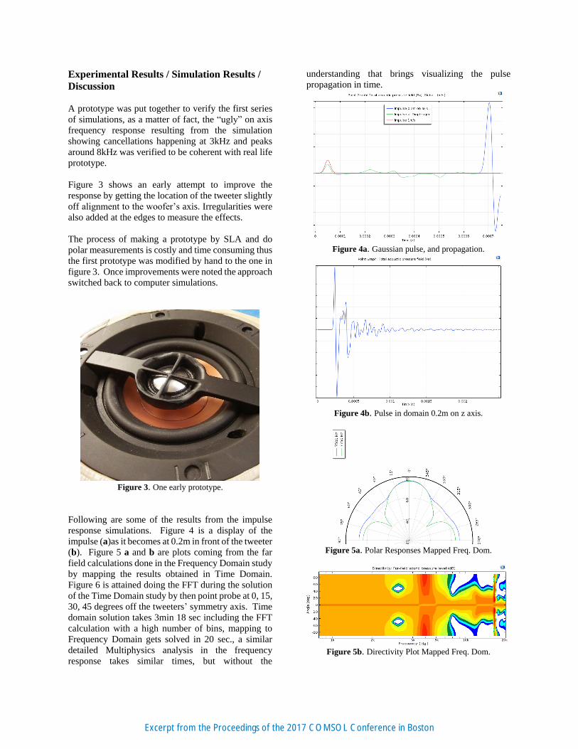
Following are some of the results from the impulse

response simulations. Figure 4 is a display of the

impulse (a)as it becomes at 0.2m in front of the tweeter

(b). Figure 5 a and b are plots coming from the far

field calculations done in the Frequency Domain study

by mapping the results obtained in Time Domain.

Figure 6 is attained doing the FFT during the solution

of the Time Domain study by then point probe at 0, 15,

30, 45 degrees off the tweeters’ symmetry axis. Time

domain solution takes 3min 18 sec including the FFT

calculation with a high number of bins, mapping to

Frequency Domain gets solved in 20 sec., a similar

detailed Multiphysics analysis in the frequency

response takes similar times, but without the

understanding that brings visualizing the pulse

propagation in time.

Figure 4a. Gaussian pulse, and propagation.

Figure 4b. Pulse in domain 0.2m on z axis.

Figure 5a. Polar Responses Mapped Freq. Dom.

Figure 5b. Directivity Plot Mapped Freq. Dom.


Figure 6. Frequency response by FFT of impulse

Now, detailed Multiphysics simulations results that

include AC/DC, Structural Mechanics and Acoustics

Modules. Figure 7a SPL and in figure 8 impedance

curves with real prototype measurements imported in

COMSOL for comparison. In figure 7b I have placed

similar resolution points as in figure 6 for comparison

to the FFT results.

Figure 7a. Frequency response detailed simulation.

Figure 7b. Frequency response at few angles.

Figure 8. Impedance, simulated vs. measured (Z)

Figure 9 a. Sound Pressure Level FFT.

Figure 9 b. Sound Pressure Level mapped results.


Figure 9 c. Sound Pressure Level Frequency Domain.

There was a good amount of correlation between the

results from studies of the impulse response to fully

fledged Multiphysics simulation, corresponding dips

and peaks, similarities in polar response etc. that show

the usefulness of this approach.

Figure 6 is an SPL response from performing an FFT

from the time domain results on axis, at 15, 30 and 45

degrees. It is nice to see that beside the attenuation in

frequency coming from the rise in frequency of the

tweeter impedance, the behavior displayed matches. In

detail, the peak at 8kHz on axis gradually becomes a

dip at 45 degrees and the same behavior is captured in

both approaches.

For an interesting subject on the PML, figure 9 shows

the SPL map of the three methodologies at 7333Hz, a

is the FFT from the time domain impulse, the domain

was kept on purpose the same among the studies and

the PLM size is smaller than recommended above for

the time domain, it is interesting to see the diffraction

waves caused by the superposition to a not fully

absorbing PML. This to show how its size needs to be

kept on consideration, that data mapped in the

Frequency Domain study is figure 9 b the PML of that

size works properly but the data from the Transient

study alters what the correct results are, nevertheless

patterns and behaviors are still somewhat coherent

with figure c which is a complete Multiphysics

simulation.

On a personal note, I love to see that standing wave

node hairline drop in SPL by the cavity behind the

tweeter. Actually, that is what causes the off-axis

irregularities (see appendix for measurements). Is also

fascinating seeing the results from the time domain,

how wave propagates bouncing off surfaces and

creating interference patterns.

Conclusions

I strongly believe that with some tweaks and perhaps

interfacing data to MATLAB and applying extra

calculations like Helmholtz-Kirkoff integral [3], or

FFT in a specific way could yield great gain in

processing time to eyeball the design with multiple

fast iterations using just the acoustic module.

Having experimented with time domain simulation in

COMSOL and its ability to do FFT, parse data and

results, allowing to be manipulated to further studies

and analysis of a design, has opened the door to great

possibilities. Study on distortion, visualization of

wave reflection and refraction on boundary, eventually

waterfall analysis, all in the virtual realm of computer

simulation are possible ideas as increasing computing

power becomes more affordable.

This methodology is perhaps at its infancy, but it has

great potential to become an essential tool as the

impulse response measurements approach is now in

the loudspeaker industry.

References

1. Klaus Riederer, Transfer function measurements in

audio, Helsinski University of Technology, Espoo,

Finland (1996)

2. Mikio Tohyama, Tsunehiko Koike, Acoustic Signal

Processing, 143-227. Academic Pross, San Diego, CA

(1998)

3. David W. Gunness, Ryan J. Mihelich,

LOUDSPEAKER ACOUSTIC FIELD

CALCULATIONS WITH APPLICATION TO

DIRECTIONAL RESPONSE MEASUREMENT,

AES 109th Convention, Los Angeles (2000)

Acknowledgements

My manager, Chris Perrins, for his continuous

support in the acquisition of COMSOL and its

needed hardware. Mads Herring Jensen at COMSOL

for his awesome technical knowledge. My wife

Nazirah Abdul for her patience on late nights at

work.


Appendix

The below shows the fruit of several simulation

iterations in 3d (nicknamed sharkfin) and the

comparison with a slightly improved version to the

simulated results shown in this paper. The original

geometry prototype was empirically “improved” to

some extents with some cut out and an off centering to

explore with direct SPL measurements if was worth to

evolve the geometry into something “originally”

better.

Above original prototype and sharkfin. On the right tweeter

assembled on system with open baffle. Below 360 degrees

measurements in anechoic chamber.


Documents

Loudspeaker Response Optimization with the aid of … · Loudspeaker Response Optimization with the aid of ... such a stimulus is not as practical due to several limitations [1