Long-term failure of glassy polymers under static loading ... · PDF fileLong-term failure of glassy polymers under static loading conditions ... 3.1.1 General observations: ... The

Long-term failure of glassy polymers under static loading conditions

Bas Raas

MT 03.15

September 2003

Thesis committee: Prof. Dr. Ir. H.E.H. Meijer (chairman) [TUE] Dr. Ir. L.E. Govaert [TUE] Dr. Ir. W.P. Vellinga [TUE] Dr. Ir. W. J. Nauta [TNO] Coaches: Dr. Ir. L.E. Govaert [TUE] Ir. E.T.J. Klompen [TUE] Dr. Ir. W. J. Nauta [TNO] Research carried out at the Department of Mechanical Engineering Eindhoven Polymer Laboratory, Eindhoven University of Technology, and at the Polymer Technology group, TNO Industrial Technology Eindhoven

- i -

Contents

Contents ................................................................................................................................................................ i

List of Symbols ................................................................................................................................................... ii

Abstract ............................................................................................................................................................... iii

Introduction ......................................................................................................................................................... 1

Experimental ....................................................................................................................................................... 2 2.1 Materials ........................................................................................................................................ 2 2.2 Techniques .................................................................................................................................... 2

2.2.1 Creep rupture tests .................................................................................................................. 2 2.2.2 Compression tests ................................................................................................................... 4 2.2.3 Tensile tests.............................................................................................................................. 4 2.2.4 Thermal & Mechanical treatments ........................................................................................ 5

Results and Discussion.................................................................................................................................... 7 3.1 Creep rupture of polycarbonate ........................................................................................ 7

3.1.1 General observations: Influence of thermal history.................................................. 7 3.1.2 Influence of molecular weight ....................................................................................... 9 3.1.3 Craze formation ............................................................................................................ 11

3.2 Modelling of creep rupture ............................................................................................... 12 3.3 Tough-to-brittle transition in creep rupture .................................................................... 16

3.3.1 Origin.............................................................................................................................. 16 3.3.2 Ageing Kinetics: Influence of temperature................................................................ 19 3.3.3 Ageing Kinetics: Influence of stress........................................................................... 23

Conclusions and Recommendations .......................................................................................................... 26 4.1 Conclusions .................................................................................................................. 26 4.2 Recommendations ....................................................................................................... 26

Bibliography ...................................................................................................................................................... 27

Time temperature shifting and Time stress shifting ............................................................................... 28

The Leonov model ........................................................................................................................................... 29

- ii -

List of Symbols

Symbol Description units A Cross section area [mm2] t Real time [s] F Force [N] � Stress [MPa] �y Yield stress [MPa] �l Elongation [mm] l0 Initial length [mm] � Strain [-] T Temperature [K] �H Activation Energy [J/mole] �* Activation volume [m3/mole] a(T) Temperature shift factor [-] a(�) Stress shift factor [-] C0 Fit parameter [-] C 1 Slope [MPa s-1] t a Initial age [hrs] R Universal gas constant (=8.314) [J/Mole K]

- iii -

Abstract This report deals with the prediction of long-term behaviour of polycarbonate under the application of constant stresses.

Creep rupture is governed by the same failure mechanism as tensile testing: plastic deformation. Annealing of the polycarbonate samples increases the resistance against creep rupture, as the yield stress increases. Therefore a higher applied stress is required in order to fail the sample at the same time scale as it does for quenched samples. The plastic deformation in the creep rupture experiments is found to be unaffected by differences in molecular weight. However, embrittlement occurs on low molecular weight polycarbonate. Craze initiation is found to be independent of molecular weight. Fully crazed samples still show moderate toughness during creep, which excludes craze formation as a brittle initiator.

As creep rupture proves to be governed by plastic deformation, the Leonov model is used to predict long-term creep failure. Due to a too pronounced softening behaviour, inherited by the used model, creep rupture is predicted too early. However, the slopes of the creep rupture curves are captured very well. Embrittlement is not predicted, as the Leonov model has no failure criterion built in. The embrittlement is believed to be caused by changing material properties. It is shown that creep loading enhances ageing in the same way as thermal treatments: it increases the yield stress. Embrittlement seems to be governed by the maximum tensile strength and is therefore molecular weight dependent. The increase in yield stress upon thermal annealing and creep loading can be described by a single master curve. This master curve is fitted by a single equation and a single set of parameters, which proves to be usable for all investigated polycarbonate grades.

keywords: polycarbonate, creep rupture, embrittlement, craze initiation, annealing, Leonov model

- 1 -

Chapter 1

Introduction In the past, polymers were primarily used in low-end products, such as plastic bags, food packaging, throw away cans, etcetera. Due to improved material performance, the use of polymers is now steadily increasing towards mechanically more sophisticated areas. The increasing demand of lightweight, mass produced, complex shaped products suits polymer materials very well. Nowadays polymers are used in bullet resistance vests, break layers in tyres, car panels, pipe systems, etcetera. However, a major concern of using these materials is the time-dependency of their mechanical behaviour, e.g. creep under a constant load. Taking this in account, polymers are a very difficult kind of material for designing products with a low tolerance for shape deviation. At higher load levels, besides creep, plastic yielding may occur, which further complicates the time-dependent behaviour of the polymer, as it will lead to time dependent failure phenomena known as creep rupture. Both creep and creep rupture are known to be influenced by factors such as the applied stress levels, temperature and environment. The components described previously have life spans which vary from several months up to several decades. Empirical testing of the behaviour or use of prototypes seems suitable for a period of a couple of months, but in the case of several decades, testing and prototyping are hardly applicable. Understanding of the micro structural process during deformation and prediction of this behaviour by modelling helps polymers to be more accessible for the mechanically more sophisticated areas of engineering. The Leonov model [1, 2, 3] proved to be an adequate tool to predict short term tensile behaviour of glassy polymers. The goal of this research was to investigate the long term behaviour of polycarbonate under the influence of a constant load and whether this behaviour can be applied in models, like the Leonov model.

- 2 -

Chapter 2

Experimental 2.1 Materials In order to investigate the creep rupture behaviour of polycarbonate, various grades of this material have been used. Table 2.1 shows the grades used and its variety in molecular weight.

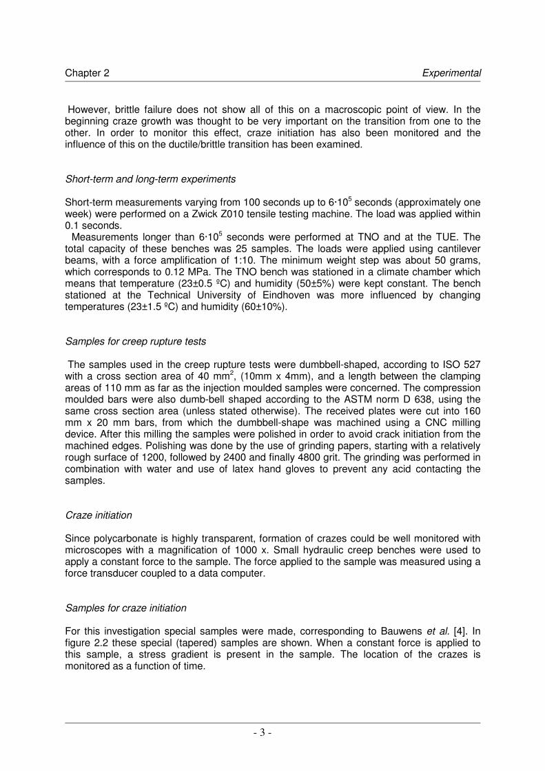
Polymer, commercial name Manufacturer Mn [g/mol] Mw [g/mol] Makrolon® CD 2000 Bayer Co. 8970 18600 Lexan® RL 3958 General Electric 9300 17000 Lexan® 101R General Electric 11600 30500 Lexan® 121R General Electric 10000 23300 Lexan® 141R General Electric 11650 25700 Lexan® 161R General Electric 12000 27700

Table 2.1: Molecular weight of the polycarbonate grades used in this study. All samples were processed from granulate material. To prevent degradation during processing, the material was dried for 24 hours under vacuum at 120 ºC. Two methods to produce samples of polycarbonate were used: injection moulding and compression moulding.

Injection moulded samples were produced according to ISO 527 with a mould temperature of 25 ºC (unless stated otherwise). Samples made with injection moulding needed no further crafting.

Compression moulded samples were made as follows: First granulate material was put in a mould, which consisted of a hardened steel plate (various thickness), with dimensions 160x160mm2. This mould was packed between two stainless steel plates covered with an aluminium foil with a thickness of 0.2 mm. The aluminium foil was used in order to prevent sticking of polycarbonate to the plates. Next the described package was heated up to 100 ºC above their Tg (approximately 150 ºC), for 15 minutes, followed by pressing of the package at a constant force of 300 kN for 5 minutes. Finally the package was cooled in a cooled press for 15 minutes under application of a force of 100 kN. 2.2 Techniques 2.2.1 Creep rupture tests Creep test were conducted on as received (1) polycarbonate samples as well as on thermal treated polycarbonate samples. When stresses were applied to these samples two failure modes could be expected: tough failure and brittle failure. Tough failure is characterised by plastic deformation and necking of the sample before it breaks.

(1) samples taken directly from the production, without any thermal-mechanical treatment

Chapter 2 Experimental

- 3 -

However, brittle failure does not show all of this on a macroscopic point of view. In the beginning craze growth was thought to be very important on the transition from one to the other. In order to monitor this effect, craze initiation has also been monitored and the influence of this on the ductile/brittle transition has been examined. Short-term and long-term experiments Short-term measurements varying from 100 seconds up to 6·105 seconds (approximately one week) were performed on a Zwick Z010 tensile testing machine. The load was applied within 0.1 seconds.

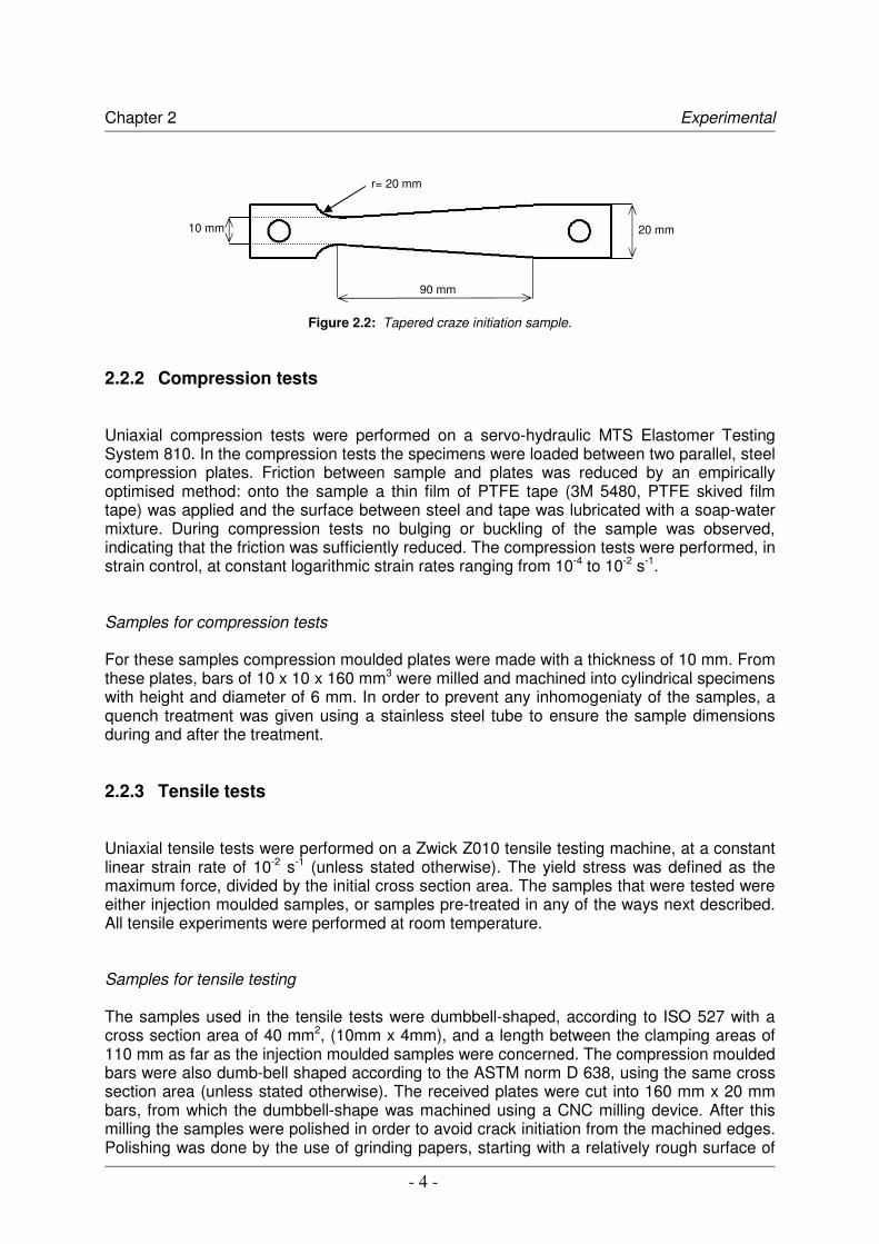
Measurements longer than 6·105 seconds were performed at TNO and at the TUE. The total capacity of these benches was 25 samples. The loads were applied using cantilever beams, with a force amplification of 1:10. The minimum weight step was about 50 grams, which corresponds to 0.12 MPa. The TNO bench was stationed in a climate chamber which means that temperature (23±0.5 ºC) and humidity (50±5%) were kept constant. The bench stationed at the Technical University of Eindhoven was more influenced by changing temperatures (23±1.5 ºC) and humidity (60±10%). Samples for creep rupture tests The samples used in the creep rupture tests were dumbbell-shaped, according to ISO 527 with a cross section area of 40 mm2, (10mm x 4mm), and a length between the clamping areas of 110 mm as far as the injection moulded samples were concerned. The compression moulded bars were also dumb-bell shaped according to the ASTM norm D 638, using the same cross section area (unless stated otherwise). The received plates were cut into 160 mm x 20 mm bars, from which the dumbbell-shape was machined using a CNC milling device. After this milling the samples were polished in order to avoid crack initiation from the machined edges. Polishing was done by the use of grinding papers, starting with a relatively rough surface of 1200, followed by 2400 and finally 4800 grit. The grinding was performed in combination with water and use of latex hand gloves to prevent any acid contacting the samples. Craze initiation Since polycarbonate is highly transparent, formation of crazes could be well monitored with microscopes with a magnification of 1000 x. Small hydraulic creep benches were used to apply a constant force to the sample. The force applied to the sample was measured using a force transducer coupled to a data computer. Samples for craze initiation For this investigation special samples were made, corresponding to Bauwens et al. [4]. In figure 2.2 these special (tapered) samples are shown. When a constant force is applied to this sample, a stress gradient is present in the sample. The location of the crazes is monitored as a function of time.


- 4 -

Figure 2.2: Tapered craze initiation sample.

2.2.2 Compression tests Uniaxial compression tests were performed on a servo-hydraulic MTS Elastomer Testing System 810. In the compression tests the specimens were loaded between two parallel, steel compression plates. Friction between sample and plates was reduced by an empirically optimised method: onto the sample a thin film of PTFE tape (3M 5480, PTFE skived film tape) was applied and the surface between steel and tape was lubricated with a soap-water mixture. During compression tests no bulging or buckling of the sample was observed, indicating that the friction was sufficiently reduced. The compression tests were performed, in strain control, at constant logarithmic strain rates ranging from 10-4 to 10-2 s-1. Samples for compression tests For these samples compression moulded plates were made with a thickness of 10 mm. From these plates, bars of 10 x 10 x 160 mm3 were milled and machined into cylindrical specimens with height and diameter of 6 mm. In order to prevent any inhomogeniaty of the samples, a quench treatment was given using a stainless steel tube to ensure the sample dimensions during and after the treatment. 2.2.3 Tensile tests Uniaxial tensile tests were performed on a Zwick Z010 tensile testing machine, at a constant linear strain rate of 10-2 s-1 (unless stated otherwise). The yield stress was defined as the maximum force, divided by the initial cross section area. The samples that were tested were either injection moulded samples, or samples pre-treated in any of the ways next described. All tensile experiments were performed at room temperature. Samples for tensile testing The samples used in the tensile tests were dumbbell-shaped, according to ISO 527 with a cross section area of 40 mm2, (10mm x 4mm), and a length between the clamping areas of 110 mm as far as the injection moulded samples were concerned. The compression moulded bars were also dumb-bell shaped according to the ASTM norm D 638, using the same cross section area (unless stated otherwise). The received plates were cut into 160 mm x 20 mm bars, from which the dumbbell-shape was machined using a CNC milling device. After this milling the samples were polished in order to avoid crack initiation from the machined edges. Polishing was done by the use of grinding papers, starting with a relatively rough surface of

r= 20 mm

90 mm

20 mm 10 mm


- 5 -

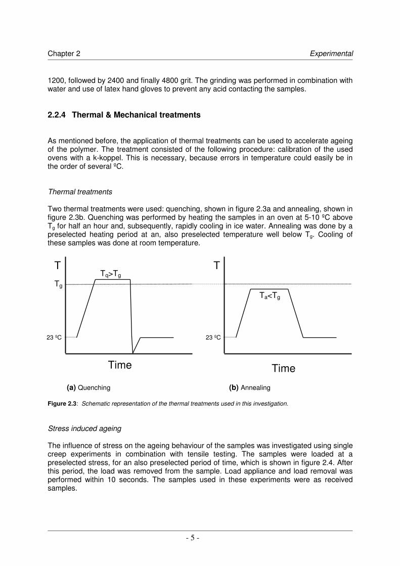
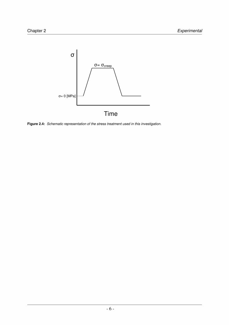
1200, followed by 2400 and finally 4800 grit. The grinding was performed in combination with water and use of latex hand gloves to prevent any acid contacting the samples. 2.2.4 Thermal & Mechanical treatments As mentioned before, the application of thermal treatments can be used to accelerate ageing of the polymer. The treatment consisted of the following procedure: calibration of the used ovens with a k-koppel. This is necessary, because errors in temperature could easily be in the order of several ºC. Thermal treatments Two thermal treatments were used: quenching, shown in figure 2.3a and annealing, shown in figure 2.3b. Quenching was performed by heating the samples in an oven at 5-10 ºC above Tg for half an hour and, subsequently, rapidly cooling in ice water. Annealing was done by a preselected heating period at an, also preselected temperature well below Tg. Cooling of these samples was done at room temperature. (a) Quenching (b) Annealing Figure 2.3: Schematic representation of the thermal treatments used in this investigation. Stress induced ageing The influence of stress on the ageing behaviour of the samples was investigated using single creep experiments in combination with tensile testing. The samples were loaded at a preselected stress, for an also preselected period of time, which is shown in figure 2.4. After this period, the load was removed from the sample. Load appliance and load removal was performed within 10 seconds. The samples used in these experiments were as received samples.

Ta<Tg

T

Time

23 ºC

Time

Tq>Tg T

23 ºC

Tg


- 6 -

Figure 2.4: Schematic representation of the stress treatment used in this investigation.

�

Time

�= 0 [MPa]

�= �creep

- 7 -

Chapter 3

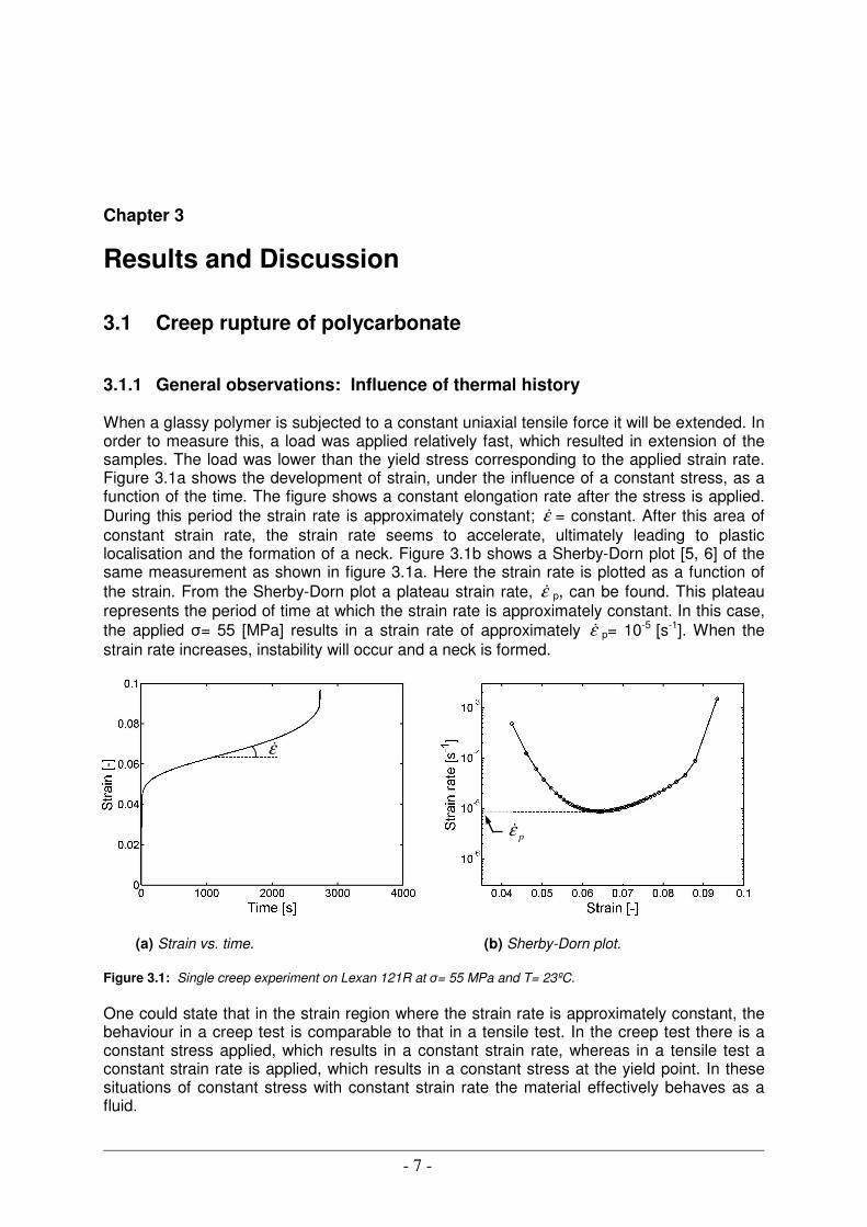
Results and Discussion 3.1 Creep rupture of polycarbonate 3.1.1 General observations: Influence of thermal history When a glassy polymer is subjected to a constant uniaxial tensile force it will be extended. In order to measure this, a load was applied relatively fast, which resulted in extension of the samples. The load was lower than the yield stress corresponding to the applied strain rate. Figure 3.1a shows the development of strain, under the influence of a constant stress, as a function of the time. The figure shows a constant elongation rate after the stress is applied. During this period the strain rate is approximately constant; ε� = constant. After this area of constant strain rate, the strain rate seems to accelerate, ultimately leading to plastic localisation and the formation of a neck. Figure 3.1b shows a Sherby-Dorn plot [5, 6] of the same measurement as shown in figure 3.1a. Here the strain rate is plotted as a function of the strain. From the Sherby-Dorn plot a plateau strain rate, ε� p, can be found. This plateau represents the period of time at which the strain rate is approximately constant. In this case, the applied �= 55 [MPa] results in a strain rate of approximately ε� p= 10-5 [s-1]. When the strain rate increases, instability will occur and a neck is formed. (a) Strain vs. time. (b) Sherby-Dorn plot. Figure 3.1: Single creep experiment on Lexan 121R at �= 55 MPa and T= 23ºC. One could state that in the strain region where the strain rate is approximately constant, the behaviour in a creep test is comparable to that in a tensile test. In the creep test there is a constant stress applied, which results in a constant strain rate, whereas in a tensile test a constant strain rate is applied, which results in a constant stress at the yield point. In these situations of constant stress with constant strain rate the material effectively behaves as a fluid.

ε�

pε�

cε

Chapter 3 Results and Discussion

- 8 -

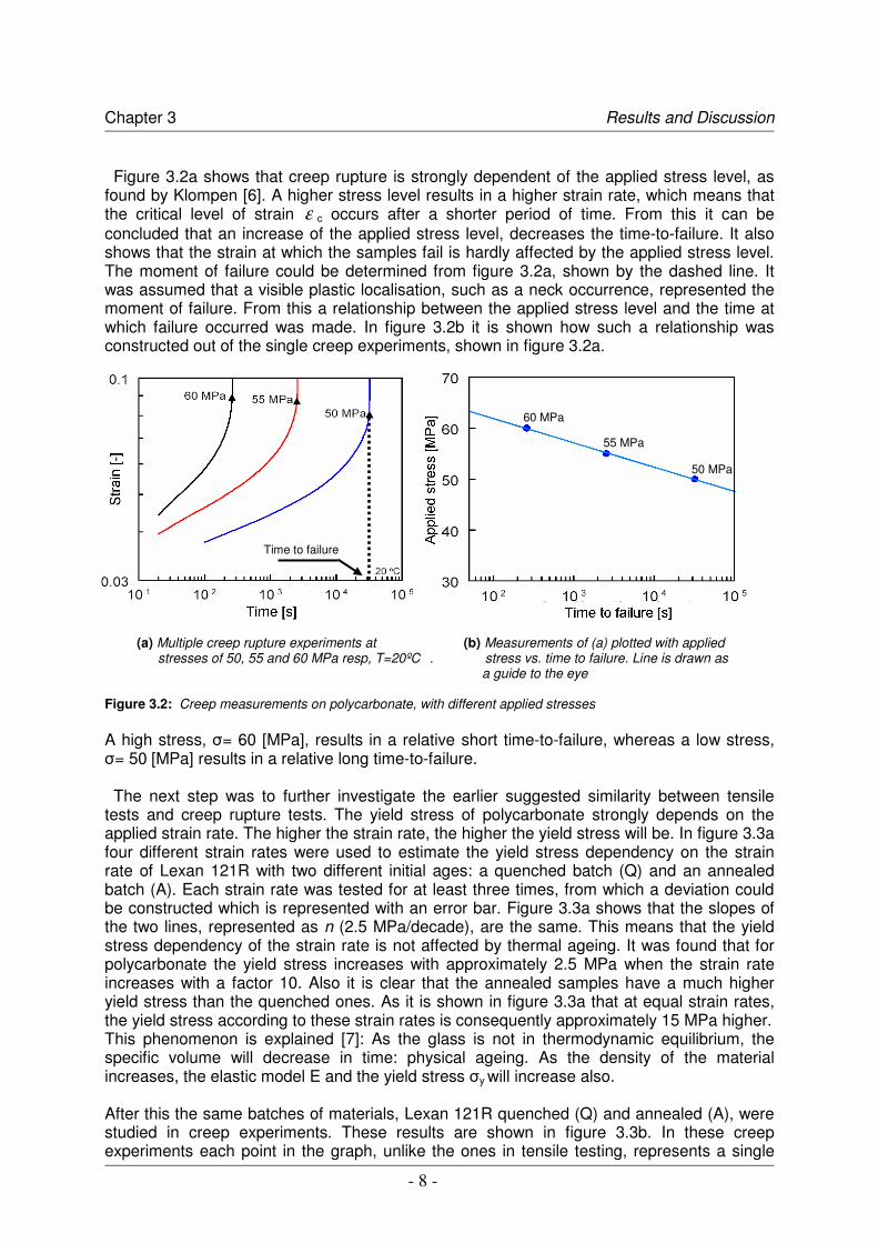
Figure 3.2a shows that creep rupture is strongly dependent of the applied stress level, as found by Klompen [6]. A higher stress level results in a higher strain rate, which means that the critical level of strain ε c occurs after a shorter period of time. From this it can be concluded that an increase of the applied stress level, decreases the time-to-failure. It also shows that the strain at which the samples fail is hardly affected by the applied stress level. The moment of failure could be determined from figure 3.2a, shown by the dashed line. It was assumed that a visible plastic localisation, such as a neck occurrence, represented the moment of failure. From this a relationship between the applied stress level and the time at which failure occurred was made. In figure 3.2b it is shown how such a relationship was constructed out of the single creep experiments, shown in figure 3.2a. (a) Multiple creep rupture experiments at (b) Measurements of (a) plotted with applied stresses of 50, 55 and 60 MPa resp, T=20ºC . stress vs. time to failure. Line is drawn as

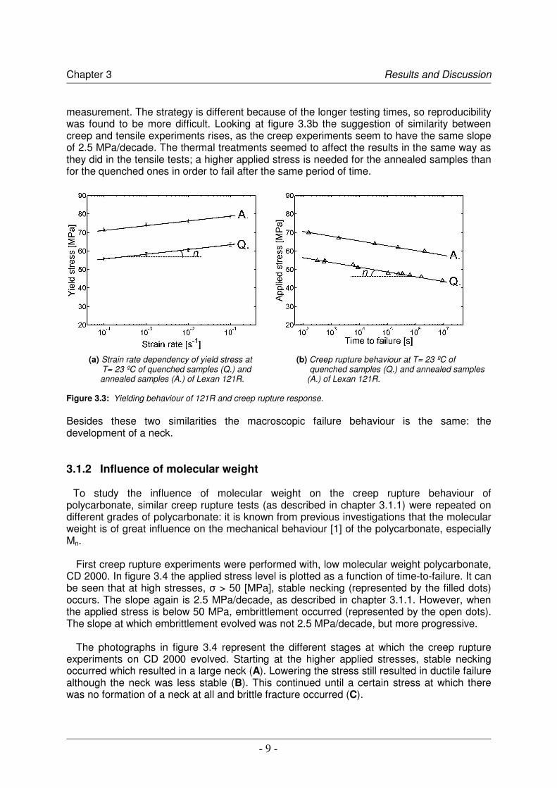
a guide to the eye Figure 3.2: Creep measurements on polycarbonate, with different applied stresses A high stress, �= 60 [MPa], results in a relative short time-to-failure, whereas a low stress, �= 50 [MPa] results in a relative long time-to-failure. The next step was to further investigate the earlier suggested similarity between tensile tests and creep rupture tests. The yield stress of polycarbonate strongly depends on the applied strain rate. The higher the strain rate, the higher the yield stress will be. In figure 3.3a four different strain rates were used to estimate the yield stress dependency on the strain rate of Lexan 121R with two different initial ages: a quenched batch (Q) and an annealed batch (A). Each strain rate was tested for at least three times, from which a deviation could be constructed which is represented with an error bar. Figure 3.3a shows that the slopes of the two lines, represented as n (2.5 MPa/decade), are the same. This means that the yield stress dependency of the strain rate is not affected by thermal ageing. It was found that for polycarbonate the yield stress increases with approximately 2.5 MPa when the strain rate increases with a factor 10. Also it is clear that the annealed samples have a much higher yield stress than the quenched ones. As it is shown in figure 3.3a that at equal strain rates, the yield stress according to these strain rates is consequently approximately 15 MPa higher. This phenomenon is explained [7]: As the glass is not in thermodynamic equilibrium, the specific volume will decrease in time: physical ageing. As the density of the material increases, the elastic model E and the yield stress �y will increase also. After this the same batches of materials, Lexan 121R quenched (Q) and annealed (A), were studied in creep experiments. These results are shown in figure 3.3b. In these creep experiments each point in the graph, unlike the ones in tensile testing, represents a single

Time to failure

60 MPa

50 MPa

55 MPa


- 9 -

measurement. The strategy is different because of the longer testing times, so reproducibility was found to be more difficult. Looking at figure 3.3b the suggestion of similarity between creep and tensile experiments rises, as the creep experiments seem to have the same slope of 2.5 MPa/decade. The thermal treatments seemed to affect the results in the same way as they did in the tensile tests; a higher applied stress is needed for the annealed samples than for the quenched ones in order to fail after the same period of time. (a) Strain rate dependency of yield stress at (b) Creep rupture behaviour at T= 23 ºC of T= 23 ºC of quenched samples (Q.) and quenched samples (Q.) and annealed samples annealed samples (A.) of Lexan 121R. (A.) of Lexan 121R. Figure 3.3: Yielding behaviour of 121R and creep rupture response. Besides these two similarities the macroscopic failure behaviour is the same: the development of a neck. 3.1.2 Influence of molecular weight

To study the influence of molecular weight on the creep rupture behaviour of polycarbonate, similar creep rupture tests (as described in chapter 3.1.1) were repeated on different grades of polycarbonate: it is known from previous investigations that the molecular weight is of great influence on the mechanical behaviour [1] of the polycarbonate, especially Mn.

First creep rupture experiments were performed with, low molecular weight polycarbonate,

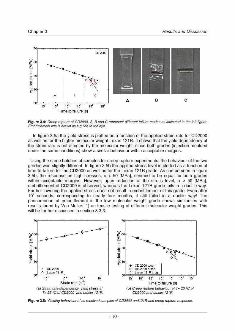
CD 2000. In figure 3.4 the applied stress level is plotted as a function of time-to-failure. It can be seen that at high stresses, � > 50 [MPa], stable necking (represented by the filled dots) occurs. The slope again is 2.5 MPa/decade, as described in chapter 3.1.1. However, when the applied stress is below 50 MPa, embrittlement occurred (represented by the open dots). The slope at which embrittlement evolved was not 2.5 MPa/decade, but more progressive.

The photographs in figure 3.4 represent the different stages at which the creep rupture

experiments on CD 2000 evolved. Starting at the higher applied stresses, stable necking occurred which resulted in a large neck (A). Lowering the stress still resulted in ductile failure although the neck was less stable (B). This continued until a certain stress at which there was no formation of a neck at all and brittle fracture occurred (C).


- 10 -

Figure 3.4: Creep rupture of CD2000. A, B and C represent different failure modes as indicated in the left figure. Embrittlement line is drawn as a guide to the eye. In figure 3.5a the yield stress is plotted as a function of the applied strain rate for CD2000 as well as for the higher molecular weight Lexan 121R. It shows that the yield dependency of the strain rate is not affected by the molecular weight, since both grades (injection moulded under the same conditions) show a similar behaviour within acceptable margins. Using the same batches of samples for creep rupture experiments, the behaviour of the two grades was slightly different. In figure 3.5b the applied stress level is plotted as a function of time-to-failure for the CD2000 as well as for the Lexan 121R grade. As can be seen in figure 3.5b, the response on high stresses, � > 50 [MPa], seemed to be equal for both grades within acceptable margins. However, upon reduction of the stress level, � < 50 [MPa], embrittlement of CD2000 is observed, whereas the Lexan 121R grade fails in a ductile way. Further lowering the applied stress does not result in embrittlement of this grade. Even after 107 seconds, corresponding to nearly four months, it still failed in a ductile way! The phenomenon of embrittlement in the low molecular weight grade shows similarities with results found by Van Melick [1] on tensile testing of different molecular weight grades. This will be further discussed in section 3.3.3.

(a) Strain rate dependency yield stress at (b) Creep rupture behaviour at T= 23 ºC of T= 23 ºC of CD2000 and Lexan 121R. CD2000 and Lexan 121R.

Figure 3.5: Yielding behaviour of as received samples of CD2000 and121R and creep rupture response.

A B C


- 11 -

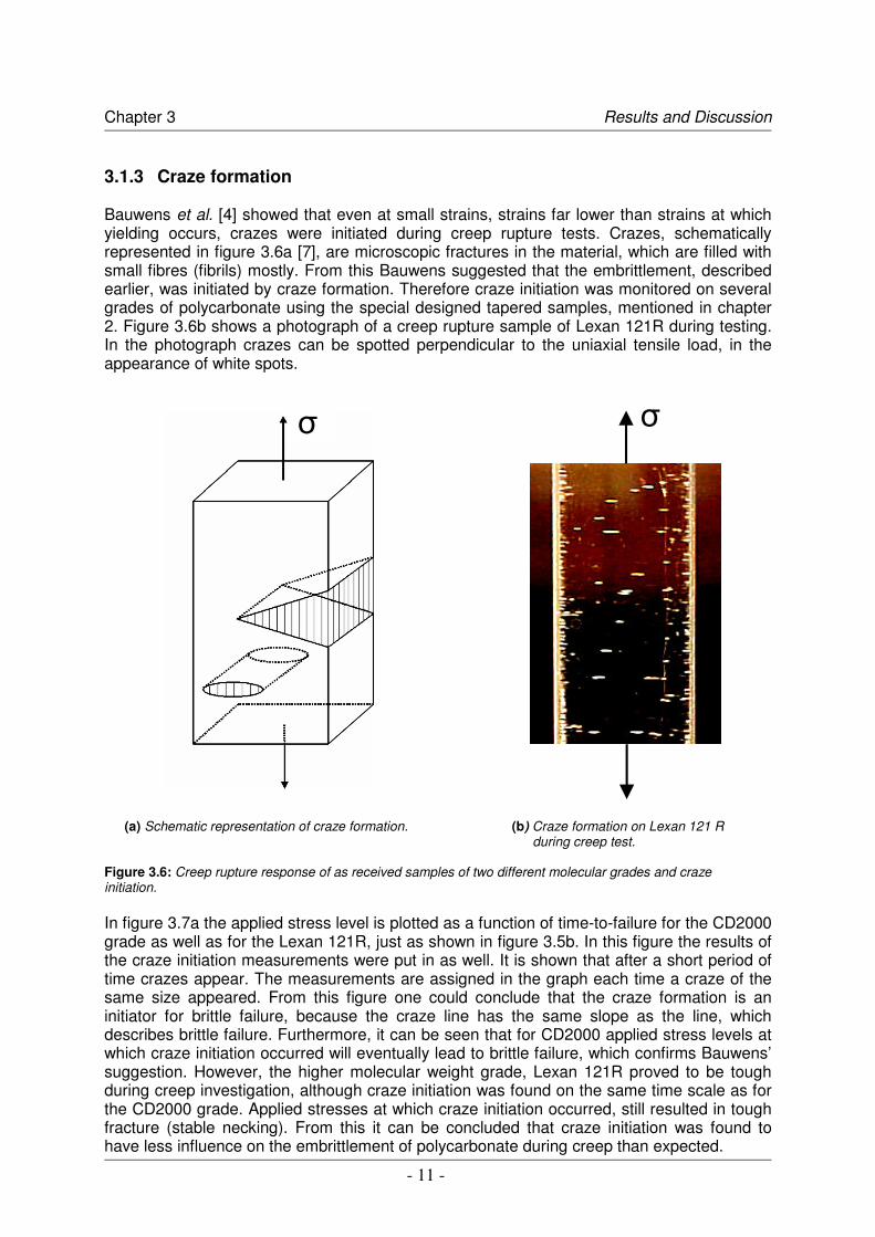
3.1.3 Craze formation Bauwens et al. [4] showed that even at small strains, strains far lower than strains at which yielding occurs, crazes were initiated during creep rupture tests. Crazes, schematically represented in figure 3.6a [7], are microscopic fractures in the material, which are filled with small fibres (fibrils) mostly. From this Bauwens suggested that the embrittlement, described earlier, was initiated by craze formation. Therefore craze initiation was monitored on several grades of polycarbonate using the special designed tapered samples, mentioned in chapter 2. Figure 3.6b shows a photograph of a creep rupture sample of Lexan 121R during testing. In the photograph crazes can be spotted perpendicular to the uniaxial tensile load, in the appearance of white spots.

(a) Schematic representation of craze formation. (b) Craze formation on Lexan 121 R during creep test.

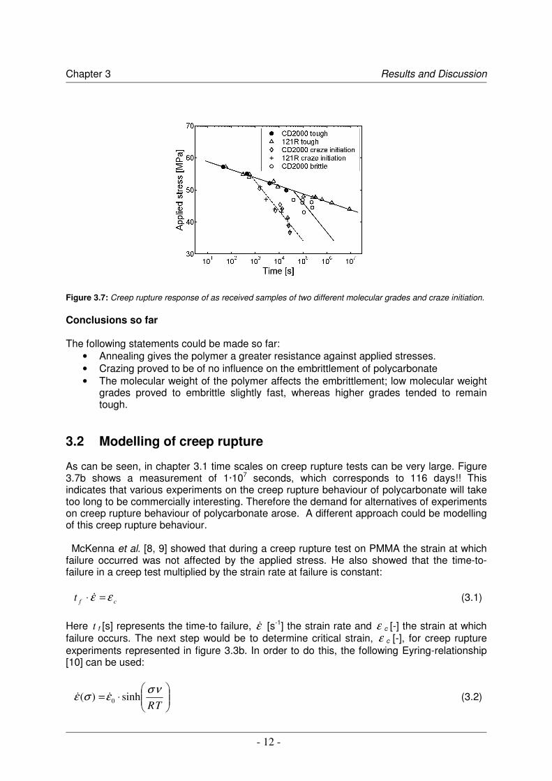
Figure 3.6: Creep rupture response of as received samples of two different molecular grades and craze initiation. In figure 3.7a the applied stress level is plotted as a function of time-to-failure for the CD2000 grade as well as for the Lexan 121R, just as shown in figure 3.5b. In this figure the results of the craze initiation measurements were put in as well. It is shown that after a short period of time crazes appear. The measurements are assigned in the graph each time a craze of the same size appeared. From this figure one could conclude that the craze formation is an initiator for brittle failure, because the craze line has the same slope as the line, which describes brittle failure. Furthermore, it can be seen that for CD2000 applied stress levels at which craze initiation occurred will eventually lead to brittle failure, which confirms Bauwens’ suggestion. However, the higher molecular weight grade, Lexan 121R proved to be tough during creep investigation, although craze initiation was found on the same time scale as for the CD2000 grade. Applied stresses at which craze initiation occurred, still resulted in tough fracture (stable necking). From this it can be concluded that craze initiation was found to have less influence on the embrittlement of polycarbonate during creep than expected.

� �


- 12 -

Figure 3.7: Creep rupture response of as received samples of two different molecular grades and craze initiation. Conclusions so far The following statements could be made so far:

• Annealing gives the polymer a greater resistance against applied stresses. • Crazing proved to be of no influence on the embrittlement of polycarbonate • The molecular weight of the polymer affects the embrittlement; low molecular weight

grades proved to embrittle slightly fast, whereas higher grades tended to remain tough.

3.2 Modelling of creep rupture As can be seen, in chapter 3.1 time scales on creep rupture tests can be very large. Figure 3.7b shows a measurement of 1·107 seconds, which corresponds to 116 days!! This indicates that various experiments on the creep rupture behaviour of polycarbonate will take too long to be commercially interesting. Therefore the demand for alternatives of experiments on creep rupture behaviour of polycarbonate arose. A different approach could be modelling of this creep rupture behaviour. McKenna et al. [8, 9] showed that during a creep rupture test on PMMA the strain at which failure occurred was not affected by the applied stress. He also showed that the time-to-failure in a creep test multiplied by the strain rate at failure is constant:

cft εε =⋅ � (3.1)

Here t f [s] represents the time-to failure, ε� [s-1] the strain rate and ε c [-] the strain at which failure occurs. The next step would be to determine critical strain, ε c [-], for creep rupture experiments represented in figure 3.3b. In order to do this, the following Eyring-relationship [10] can be used:

��

��

�⋅=

TRνσεσε sinh)( 0�� (3.2)


- 13 -

Here ε� [s-1] represents the strain rate as a function of the stress σ [MPa], ε� 0 [s-1] the strain rate, ν the activation volume [m3], R the universal gas constant [J/mole K] and T [K] the temperature.

This can be rewritten, assuming sinh(x) � 0.5exp(x) for large x and 0σ =TR

ν:

)(exp2

)(0

0

σσεσε ⋅=

�� (3.3)

Equation 3.3 can also be written as:

��

��

�⋅=

00

2ln)(

εεσεσ�

�� (3.4)

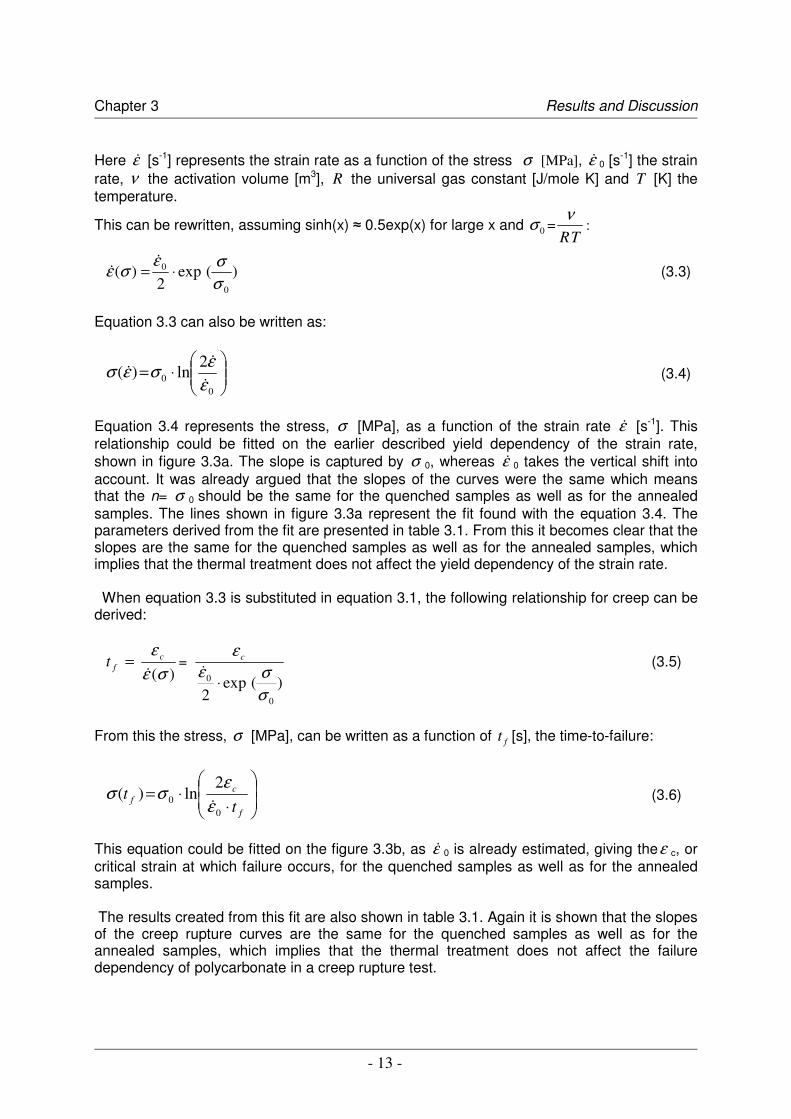
Equation 3.4 represents the stress, σ [MPa], as a function of the strain rate ε� [s-1]. This relationship could be fitted on the earlier described yield dependency of the strain rate, shown in figure 3.3a. The slope is captured by σ 0, whereas ε� 0 takes the vertical shift into account. It was already argued that the slopes of the curves were the same which means that the n= σ 0 should be the same for the quenched samples as well as for the annealed samples. The lines shown in figure 3.3a represent the fit found with the equation 3.4. The parameters derived from the fit are presented in table 3.1. From this it becomes clear that the slopes are the same for the quenched samples as well as for the annealed samples, which implies that the thermal treatment does not affect the yield dependency of the strain rate. When equation 3.3 is substituted in equation 3.1, the following relationship for creep can be derived:

)(σεε�

cft = =

)(exp2 0

0

σσε

ε

⋅�

c (3.5)

From this the stress, σ [MPa], can be written as a function of ft [s], the time-to-failure:

��

�

�

��

�

�

⋅⋅=

f

cf t

t0

0

2ln)(

εεσσ

� (3.6)

This equation could be fitted on the figure 3.3b, as ε� 0 is already estimated, giving theε c, or critical strain at which failure occurs, for the quenched samples as well as for the annealed samples. The results created from this fit are also shown in table 3.1. Again it is shown that the slopes of the creep rupture curves are the same for the quenched samples as well as for the annealed samples, which implies that the thermal treatment does not affect the failure dependency of polycarbonate in a creep rupture test.


- 14 -

Table 3.1: Parameter set for tensile and creep rupture. Table 3.1 shows that ε c differs significantly for the two initial ages. McKenna et al. [8, 9] also noticed a change in ε c and stated that equation 3.1 is valid for any given ageing time. He mentioned that ε c changes at long ageing times and argued that this was caused by chemical degradation, as this was evidenced by significant changes in molecular weight. However this argument implies that two different grades of polycarbonate, with the same initial condition, should have a different response to a creep rupture test. As shown in figure 3.5 two different molecular weight grades of polycarbonate with the same initial conditions, CD2000 and Lexan 121R, both respond in the same way to a creep rupture test. The CD2000 grade eventually turns brittle, but the model takes only the ductile (yielding) failures into account. The conclusions made by McKenna concerning the influence of changes in molecular weight on the creep rupture behaviour should therefore be questioned. An other reason for this could be the fact that McKenna used PMMA instead of polycarbonate in his investigation. PMMA is known to age much less progressive according to thermal treatments. Modelling of creep rupture experiments by the use of equation 3.1 is not so effective for reducing experimental times, because of the changing ε c. Due to differences in initial conditions, creep rupture data are always required to predict the long term behaviour in a creep rupture test.

An other way of predicting creep rupture of polycarbonate could be constitutive modelling.

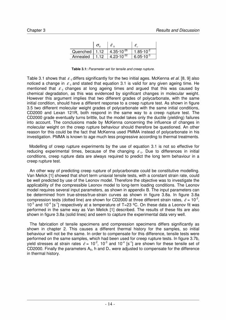
Van Melick [1] showed that short term uniaxial tensile tests, with a constant strain rate, could be well predicted by use of the Leonov model. Therefore the objective was to investigate the applicability of the compressible Leonov model to long-term loading conditions. The Leonov model requires several input parameters, as shown in appendix B. The input parameters can be determined from true-stress/true-strain curves as shown in figure 3.8a. In figure 3.8a compression tests (dotted line) are shown for CD2000 at three different strain rates, ε� = 10-2, 10-3 and 10-4 [s-1] respectively at a temperature of T=23 ºC. On these data a Leonov fit was performed in the same way as Van Melick [1] described. The results of these fits are also shown in figure 3.8a (solid lines) and seem to capture the experimental data very well.

The fabrication of tensile specimens and compression specimens differs significantly as

shown in chapter 2. This causes a different thermal history for the samples, so initial behaviour will not be the same. In order to compensate for this difference, tensile tests were performed on the same samples, which had been used for creep rupture tests. In figure 3.7b, yield stresses at strain rates ε� = 10-2, 10-3 and 10-4 [s-1] are shown for these tensile set of CD2000. Finally the parameters A0, h and D� were adjusted to compensate for the difference in thermal history.

0σ 0ε� cε

Quenched 1.12 4.35·10-26 1.85·10-2 Annealed 1.12 4.23·10-32 6.05·10-3


- 15 -

(a) True stress vs. strain, for CD2000, at (b) Tensile yield stresses for CD2000. rates: 10-2, 10-3 and 10-4 s-1. Experiment as well as the model prediction. Figure 3.8: Behaviour of as received samples of CD2000 and 121R and creep rupture response. The final parameter set found for the CD2000 batch at which creep rupture tests had been performed is shown in table 3.2. This parameter set was put in the same Finite Element Method (FEM) as described by Van Melick [1, 2, 3]. Here FEM was used to predict short term uniaxial tests on polycarbonate and polystyrene by prescribing a constant linear strain rate, ε� = 10-3 [s-1]. In order to predict creep rupture with FEM, a constant stress is prescribed instead of a constant linear strain rate. After a certain period of time, plastic deformation of the model can be observed due to the applied stress. From this a figure in which the strain is plotted as a function of time can be created. This is shown in figure 3.1a. From this figure the time to failure as a function of the applied stress can be determined, as described earlier. To construct a figure in which the applied stress is represented as a function of the time to failure, as shown for example in figure 3.4, creep rupture tests on several levels of applied stresses were calculated. In figure 3.9 the same creep rupture test as described in figure 3.4 is shown (dots), with the addition of the results found by the FEM model. These results are shown as a solid line, which is constructed by connecting the single results from the modelling as a guide to the eye.

Table 3.2: Material parameters used Figure 3.9: Creep rupture behaviour atT= 23ºC of for simulations. CD2000; experimental (dotted) and prediction (line).

E 790 [MPa] ν 0.37 [-] τ 0 0.56 [MPa] A 0 1.4 • 1027 [sec] µ 0.075 [-] h 190 [-] D� 38 [-] G r 30 [MPa]


- 16 -

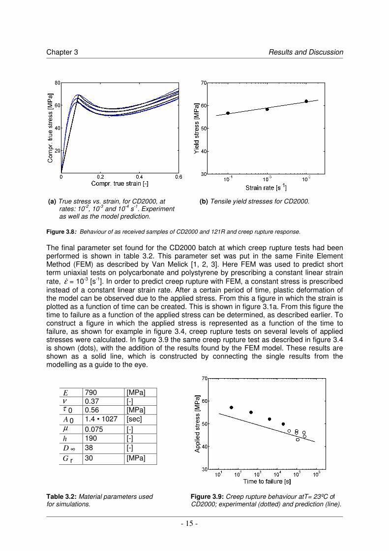
From figure 3.9, two important conclusions on the use of this model can be drawn: 1) The slope of the predicted creep rupture curve on CD2000 is captured well according to the measured creep rupture data of CD2000. However, failure occurs too early. A possible explanation for this is the use of a first order evolution of the strain softening, resulting in a too pronounced softening at the yield point. This is shown in figure 3.10, where the fit (solid line) is shown in comparison with the measured data (dotted line) at the strain rate, ε� = 10-4 [s-1]. The more pronounced softening results in a decrease in the time-to-failure, forcing the line of prediction to the left by means of a horizontal shift. In ongoing studies, Klompen et al captures the softening behaviour by the use of higher order evolution of the strain softening. Using these parameters, the predicted creep line matches the experimental data more accurately.

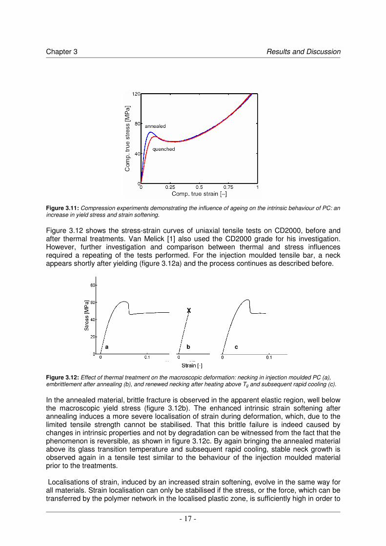
Figure 3.10: Magnified representation of the yield point of figure 3.7a at a strain rate of 10-4 s-1. 2) The model also predicts ductile failure throughout, where the experimental data show an embrittlement of CD2000. This is caused by the absence of a brittle fracture criterion in the model, which will be further discussed in chapter 3.3. 3.3 Tough-to-brittle transition in creep rupture 3.3.1 Origin During creep rupture the time-to-failure increases upon decreasing of the applied stress. So on an increasing time scale, the applied stress is decreasing which makes the implementation of a failure criterion more difficult. As the applied stress decreases a brittle fracture criterion is difficult to use. In the model the material properties stay the same throughout the whole calculation. However, this is not the case in real experiments. This was already suggested by Van Melick [1]: An increase was shown in yield stress upon thermal treatments (figure 3.11). In this figure the stress vs. strain curve is shown for an as received as well as for a annealed sample. The change in strain softening (or yield drop) equals the increase in yield stress since the large strain behaviour (strain hardening), remains unaffected by ageing. These subtle changes in strain softening prove to have major consequences for the macroscopic deformation behaviour.


- 17 -

Figure 3.11: Compression experiments demonstrating the influence of ageing on the intrinsic behaviour of PC: an increase in yield stress and strain softening. Figure 3.12 shows the stress-strain curves of uniaxial tensile tests on CD2000, before and after thermal treatments. Van Melick [1] also used the CD2000 grade for his investigation. However, further investigation and comparison between thermal and stress influences required a repeating of the tests performed. For the injection moulded tensile bar, a neck appears shortly after yielding (figure 3.12a) and the process continues as described before. Figure 3.12: Effect of thermal treatment on the macroscopic deformation: necking in injection moulded PC (a), embrittlement after annealing (b), and renewed necking after heating above Tg and subsequent rapid cooling (c). In the annealed material, brittle fracture is observed in the apparent elastic region, well below the macroscopic yield stress (figure 3.12b). The enhanced intrinsic strain softening after annealing induces a more severe localisation of strain during deformation, which, due to the limited tensile strength cannot be stabilised. That this brittle failure is indeed caused by changes in intrinsic properties and not by degradation can be witnessed from the fact that the phenomenon is reversible, as shown in figure 3.12c. By again bringing the annealed material above its glass transition temperature and subsequent rapid cooling, stable neck growth is observed again in a tensile test similar to the behaviour of the injection moulded material prior to the treatments. Localisations of strain, induced by an increased strain softening, evolve in the same way for all materials. Strain localisation can only be stabilised if the stress, or the force, which can be transferred by the polymer network in the localised plastic zone, is sufficiently high in order to

X

a c b c

X


- 18 -

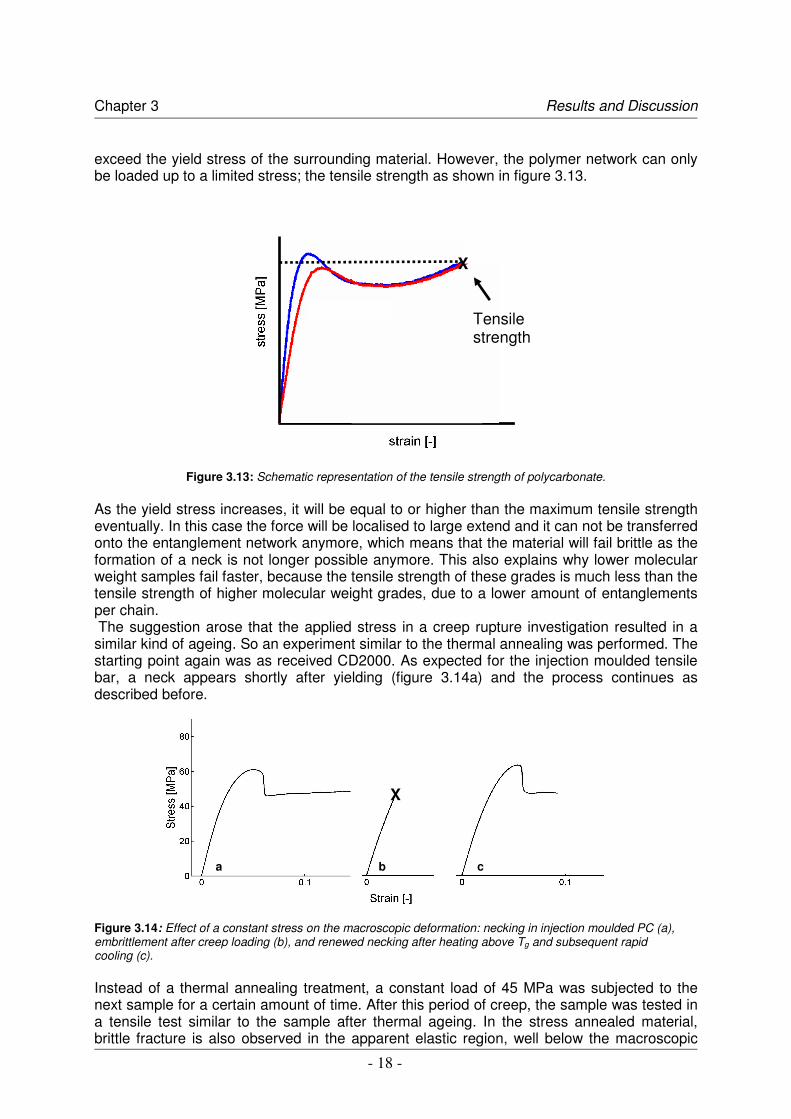
exceed the yield stress of the surrounding material. However, the polymer network can only be loaded up to a limited stress; the tensile strength as shown in figure 3.13.

Figure 3.13: Schematic representation of the tensile strength of polycarbonate. As the yield stress increases, it will be equal to or higher than the maximum tensile strength eventually. In this case the force will be localised to large extend and it can not be transferred onto the entanglement network anymore, which means that the material will fail brittle as the formation of a neck is not longer possible anymore. This also explains why lower molecular weight samples fail faster, because the tensile strength of these grades is much less than the tensile strength of higher molecular weight grades, due to a lower amount of entanglements per chain. The suggestion arose that the applied stress in a creep rupture investigation resulted in a similar kind of ageing. So an experiment similar to the thermal annealing was performed. The starting point again was as received CD2000. As expected for the injection moulded tensile bar, a neck appears shortly after yielding (figure 3.14a) and the process continues as described before. Figure 3.14: Effect of a constant stress on the macroscopic deformation: necking in injection moulded PC (a), embrittlement after creep loading (b), and renewed necking after heating above Tg and subsequent rapid cooling (c). Instead of a thermal annealing treatment, a constant load of 45 MPa was subjected to the next sample for a certain amount of time. After this period of creep, the sample was tested in a tensile test similar to the sample after thermal ageing. In the stress annealed material, brittle fracture is also observed in the apparent elastic region, well below the macroscopic

a b c

X

Tensile strength

X


- 19 -

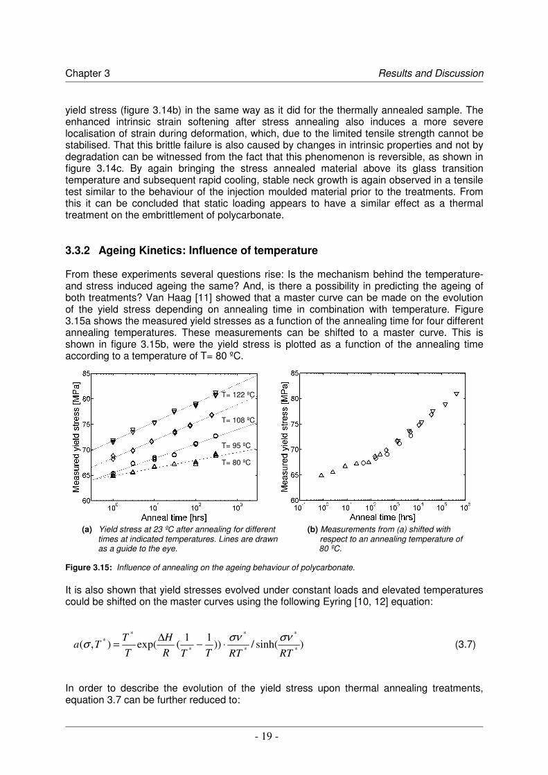
yield stress (figure 3.14b) in the same way as it did for the thermally annealed sample. The enhanced intrinsic strain softening after stress annealing also induces a more severe localisation of strain during deformation, which, due to the limited tensile strength cannot be stabilised. That this brittle failure is also caused by changes in intrinsic properties and not by degradation can be witnessed from the fact that this phenomenon is reversible, as shown in figure 3.14c. By again bringing the stress annealed material above its glass transition temperature and subsequent rapid cooling, stable neck growth is again observed in a tensile test similar to the behaviour of the injection moulded material prior to the treatments. From this it can be concluded that static loading appears to have a similar effect as a thermal treatment on the embrittlement of polycarbonate. 3.3.2 Ageing Kinetics: Influence of temperature From these experiments several questions rise: Is the mechanism behind the temperature-and stress induced ageing the same? And, is there a possibility in predicting the ageing of both treatments? Van Haag [11] showed that a master curve can be made on the evolution of the yield stress depending on annealing time in combination with temperature. Figure 3.15a shows the measured yield stresses as a function of the annealing time for four different annealing temperatures. These measurements can be shifted to a master curve. This is shown in figure 3.15b, were the yield stress is plotted as a function of the annealing time according to a temperature of T= 80 ºC.

(a) Yield stress at 23 ºC after annealing for different (b) Measurements from (a) shifted with times at indicated temperatures. Lines are drawn respect to an annealing temperature of as a guide to the eye. 80 ºC.

Figure 3.15: Influence of annealing on the ageing behaviour of polycarbonate. It is also shown that yield stresses evolved under constant loads and elevated temperatures could be shifted on the master curves using the following Eyring [10, 12] equation:

)sinh(/))11

(exp(),(*

*

*

*

*

**

RTRTTTRH

TT

Taσνσνσ ⋅−∆= (3.7)

In order to describe the evolution of the yield stress upon thermal annealing treatments, equation 3.7 can be further reduced to:

T= 122 ºC T= 108 ºC T= 95 ºC T= 80 ºC


- 20 -

))11

(exp(12

21 TTRH

a TT −∆=→ (3.8)

With this equation it becomes possible to shift yield stresses of samples with different annealing temperatures, but with the same initial age to one temperature. For example: Batch A represents as received samples of Lexan 121R and so does batch B. Both batches have the same initial age, so the yield stress measured at ε� = 10-2 is the same for both batches. Batch A is put in an oven of T= 80 ºC= 353 K and batch B is put in an oven of T= 100 ºC= 373 K. After strategically chosen times, three samples of each batch were taken from the ovens. After cooled on air for half an hour, the samples were tested at ε� = 10-2. Batch B will have a higher yield stress than batch A after the same amount of annealing time, due to the higher annealing temperature. The measurements of batch A and batch B can finally be shifted to one annealing temperature. In equation 3.8, T2 represents the temperature, which the measurements of A and B will be shifted to. T1 represents each temperature at which a batch is annealed. The main goal here is to quantify stress induced ageing. However, it was necessary to do some thermal experiments also in order to find values for �H and ν *. The results, found by the shifting, correspond to the results found by van Haag. The �H found was estimated at 2.0�105 J/mole, which is in good agreement with the 1.9�105 J/mole found by van Haag.

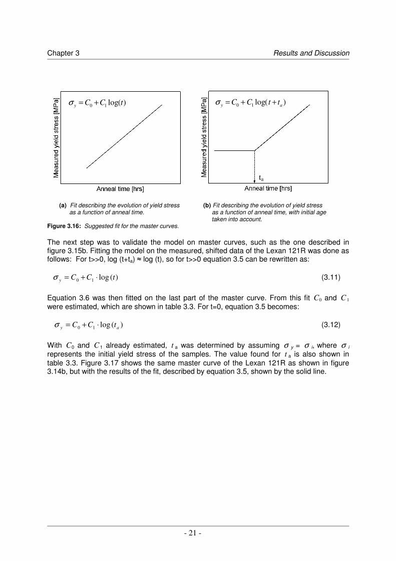
Taking a closer look at the master curve it can be seen that for large annealing times the

slope of the curve seems to become constant, while for short annealing times the slope is much less steep. Modelling this behaviour was done by assuming a line with constant slope, as can be seen in figure 3.16 a. This can be described with the following equation:

)(log10 tCCy +=σ (3.9)

Here σ y represents the yield stress [MPa], C0 [-] a constant in order to get the right vertical shift and C1 represents the slope of the line [MPa s-1]. Figure 3.16a shows the predicted master curve, which describes the evolving of the yield stress as a function of the annealing time according to one temperature. As mentioned before the master curve shows a kind of less progressive period. For a certain amount of time the yield stress hardly increases. It seems as if the material is already aged in the past, and has an initial age of its own. This age could be, for example, introduced by the production of the sample, by cooling the sample or by storage of the sample. This also suggests that complete “initial age” free samples are hard to get. However, Van Melick et al. [13] showed that by cold rolling a ‘’zero age’’ could be achieved. This cold rolling can be seen as a mechanical rejuvenation, whereas thermal quenching can be seen as thermal rejuvenation. Passing the initial age is needed to get a substantial increase in yield stress. Taking this turn point in account the fit was adapted introducing ta as an initial age:

)(log10 ay ttCC ++=σ (3.10)

Here σ y represents the yield stress [MPa], C0 [-] a constant in order to get the right vertical shift and C1 represents the slope of the line [MPa s-1] and t a the initial age of the sample in [hrs]. The result of this adaption is shown in figure 3.16 b. The yield stress is constant for the amount of annealing time at which the initial age is not passed.


- 21 -

(a) Fit describing the evolution of yield stress (b) Fit describing the evolution of yield stress as a function of anneal time. as a function of anneal time, with initial age

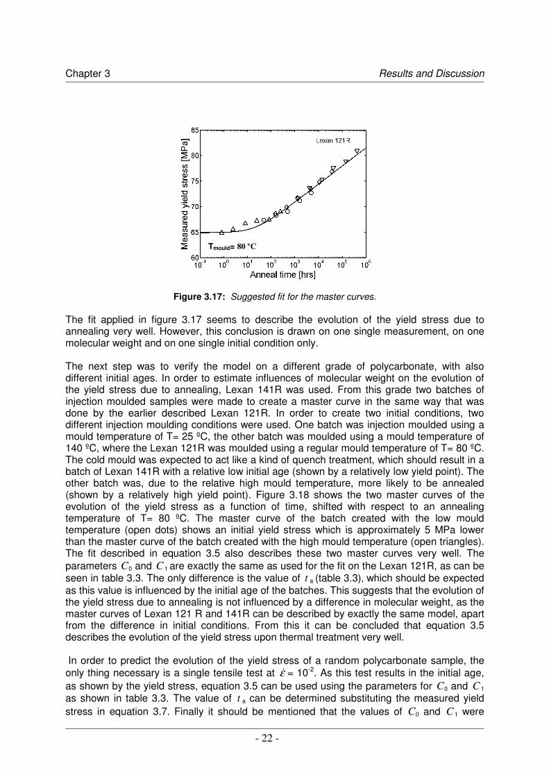
taken into account. Figure 3.16: Suggested fit for the master curves. The next step was to validate the model on master curves, such as the one described in figure 3.15b. Fitting the model on the measured, shifted data of the Lexan 121R was done as follows: For t>>0, log (t+ta) � log (t), so for t>>0 equation 3.5 can be rewritten as:

)(log10 tCCy ⋅+=σ (3.11)

Equation 3.6 was then fitted on the last part of the master curve. From this fit C0 and C 1 were estimated, which are shown in table 3.3. For t=0, equation 3.5 becomes: )(log10 ay tCC ⋅+=σ (3.12)

With C0 and C1 already estimated, t a was determined by assuming σ y = σ i, where σ i represents the initial yield stress of the samples. The value found for t a is also shown in table 3.3. Figure 3.17 shows the same master curve of the Lexan 121R as shown in figure 3.14b, but with the results of the fit, described by equation 3.5, shown by the solid line.

ta

)(log10 ay ttCC ++=σ)(log10 tCCy +=σ


- 22 -

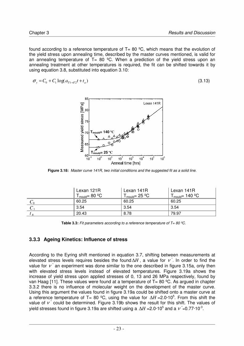
Figure 3.17: Suggested fit for the master curves. The fit applied in figure 3.17 seems to describe the evolution of the yield stress due to annealing very well. However, this conclusion is drawn on one single measurement, on one molecular weight and on one single initial condition only. The next step was to verify the model on a different grade of polycarbonate, with also different initial ages. In order to estimate influences of molecular weight on the evolution of the yield stress due to annealing, Lexan 141R was used. From this grade two batches of injection moulded samples were made to create a master curve in the same way that was done by the earlier described Lexan 121R. In order to create two initial conditions, two different injection moulding conditions were used. One batch was injection moulded using a mould temperature of T= 25 ºC, the other batch was moulded using a mould temperature of 140 ºC, where the Lexan 121R was moulded using a regular mould temperature of T= 80 ºC. The cold mould was expected to act like a kind of quench treatment, which should result in a batch of Lexan 141R with a relative low initial age (shown by a relatively low yield point). The other batch was, due to the relative high mould temperature, more likely to be annealed (shown by a relatively high yield point). Figure 3.18 shows the two master curves of the evolution of the yield stress as a function of time, shifted with respect to an annealing temperature of T= 80 ºC. The master curve of the batch created with the low mould temperature (open dots) shows an initial yield stress which is approximately 5 MPa lower than the master curve of the batch created with the high mould temperature (open triangles). The fit described in equation 3.5 also describes these two master curves very well. The parameters C0 and C 1 are exactly the same as used for the fit on the Lexan 121R, as can be seen in table 3.3. The only difference is the value of t a (table 3.3), which should be expected as this value is influenced by the initial age of the batches. This suggests that the evolution of the yield stress due to annealing is not influenced by a difference in molecular weight, as the master curves of Lexan 121 R and 141R can be described by exactly the same model, apart from the difference in initial conditions. From this it can be concluded that equation 3.5 describes the evolution of the yield stress upon thermal treatment very well. In order to predict the evolution of the yield stress of a random polycarbonate sample, the only thing necessary is a single tensile test at ε� = 10-2. As this test results in the initial age, as shown by the yield stress, equation 3.5 can be used using the parameters for C0 and C 1 as shown in table 3.3. The value of t a can be determined substituting the measured yield stress in equation 3.7. Finally it should be mentioned that the values of C0 and C 1 were

Tmould= 80 ºC


- 23 -

found according to a reference temperature of T= 80 ºC, which means that the evolution of the yield stress upon annealing time, described by the master curves mentioned, is valid for an annealing temperature of T= 80 ºC. When a prediction of the yield stress upon an annealing treatment at other temperatures is required, the fit can be shifted towards it by using equation 3.8, substituted into equation 3.10:

)(log 2110 aTTy ttaCC ++= →σ (3.13)

Figure 3.18: Master curve 141R, two initial conditions and the suggested fit as a solid line.

Lexan 121R

Tmould= 80 ºC Lexan 141R Tmould= 25 ºC

Lexan 141R Tmould= 140 ºC

C0 60.25 60.25 60.25

C 1 3.54 3.54 3.54 t a 20.43 8.78 79.97

Table 3.3: Fit parameters according to a reference temperature of T= 80 ºC.

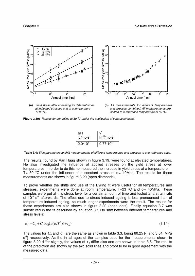
3.3.3 Ageing Kinetics: Influence of stress According to the Eyring shift mentioned in equation 3.7, shifting between measurements at elevated stress levels requires besides the found H∆ , a value for ν *. In order to find the value for ν * an experiment was done similar to the one described in figure 3.15a, only then with elevated stress levels instead of elevated temperatures. Figure 3.19a shows the increase of yield stress upon applied stresses of 0, 13 and 26 MPa respectively, found by van Haag [11]. These values were found at a temperature of T= 80 ºC. As argued in chapter 3.3.2 there is no influence of molecular weight on the development of the master curve. Using this argument the values found in figure 3.19a could be shifted onto a master curve at a reference temperature of T= 80 ºC, using the value for H∆ =2.0·105. From this shift the value of ν * could be determined. Figure 3.19b shows the result for this shift. The values of yield stresses found in figure 3.19a are shifted using a H∆ =2.0·105 and a ν *=0.77·10-3.

Tmould= 25 ºC

Tmould= 140 ºC


- 24 -

(a) Yield stress after annealing for different times (b) All measurements for different temperatures at indicated stresses and at a temperature and stresses combined. All measurements are

of 80 ºC. shifted to a reference temperature of 80 ºC.

Figure 3.19: Results for annealing at 80 ºC under the application of various stresses. Table 3.4: Shift parameters to shift measurements of different temperatures and stresses to one reference state.

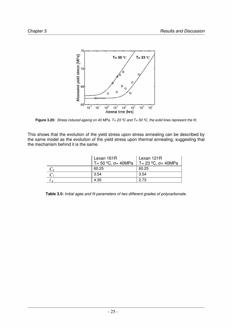
The results, found by Van Haag shown in figure 3.19, were found at elevated temperatures. He also investigated the influence of applied stresses on the yield stress at lower temperatures. In order to do this he measured the increase in yield stress at a temperature T= 50 ºC under the influence of a constant stress of �= 40Mpa. The results for these measurements are shown in figure 3.20 (open diamonds). To prove whether the shifts and use of the Eyring fit were useful for all temperatures and stresses, experiments were done at room temperature, T=23 ºC and �= 40MPa. These samples were put at this stress level for a certain amount of time and tested at a strain rate of 10-2 s-1 afterwards. The effect due to stress induced ageing is less pronounced than of temperature induced ageing, so much longer experiments were the result. The results for these experiments are also shown in figure 3.20 (open dots). Finally equation 3.7 was substituted in the fit described by equation 3.10 to shift between different temperatures and stress levels: )),((log *

10 ay ttTaCC ++= σσ (3.14) The values for C0 and C 1 are the same as shown in table 3.3, being 60.25 [-] and 3.54 [MPa s-1] respectively. As the initial ages of the samples used for the measurements shown in figure 3.20 differ slightly, the values of t a differ also and are shown in table 3.5. The results of the prediction are shown by the two solid lines and proof to be in good agreement with the measured data.

�H [J/mole]

�*

[m3/mole]

2.0·105 0.77·10-3


- 25 -

Figure 3.20: Stress induced ageing on 40 MPa, T= 23 ºC and T= 50 ºC, the solid lines represent the fit. This shows that the evolution of the yield stress upon stress annealing can be described by the same model as the evolution of the yield stress upon thermal annealing, suggesting that the mechanism behind it is the same.

Lexan 161R T= 50 ºC, �= 40MPa

Lexan 121R T= 23 ºC, �= 40MPa

C0 60.25 60.25

C 1 3.54 3.54 t a 4.30 2.73

Table 3.5: Initial ages and fit parameters of two different grades of polycarbonate.

T= 23 ºC T= 50 ºC

- 26 -

Chapter 4

Conclusions and Recommendations

4.1 Conclusions Tensile tests and creep rupture tests on the same batches of polycarbonate show that creep rupture is governed by the same mechanism as tensile testing: plastic deformation. Differences in molecular weight show no affection on the creep rupture behaviour as long as ductile failure is concerned. However, embrittlement proves to be influenced by the molecular weight, which can be explained by an increase in yield stress. The increase in yield stress leads to embrittlement due to a limited tensile strength. As low molecular weight grades have a lower tensile strength than higher molecular grades, they fail brittle at a shorter time scale. Craze initiation is found on all the tested molecular weight grades during creep rupture experiments. However, it seems to have no influence on the embrittlement of polycarbonate during creep rupture. Modelling by using the Leonov model shows promising results. The slope of the creep rupture curve is captured well. The time scale at which failure occurs is too short, which is explained by the too pronounced softening by the model. Embrittlement is not modelled, due to the absence of a brittle fracture criterion. Embrittlement during creep rupture is originated by progressive ageing in the same way as it does during thermal annealing. The kinetics of this ageing behaviour can be captured by a single master curve. One single test at ε� = 10-2 [s-1] of a polycarbonate sample reveals its initial age, which can be used to predict the evolution of the yield stress according to applied stresses and/or temperatures.

4.2 Recommendations In order to predict the creep rupture behaviour of polycarbonate, the Leonov model proved to be a promising approach. If the too pronounced softening of the model described in this report will be made more accurate, for example by using higher order evolutions for describing the softening behaviour, yielding times can expected to be in good agreement with experimental data. As the evolution of the yield stress due to creep loading occurs progressive, as described by the master curves and by the found prediction formula, the found model can be used in combination with the Leonov model. The prediction formula can be seen as a kind of fracture criterion, which can be implemented in the FEM model.

- 27 -

Bibliography [1] H.G.H. van Melick, PhD-thesis, TUE, (2002). [2] Tervoort, T.A., Smit, R.J.M., Brekelmans, W.A.M., Govaert, L.E., A constitutive Equation

for the Elasto-Viscoplastic Deformation of Glassy Polymers, Mech. Time-Dep. Mat., 1, 269 (1998).

[3] Govaert, L.E., Timmermans, P.H.M., Brekelmans, W.A.M., J. Eng. Mat. Tech., 122, 177

(2000). [4] N. Verheulpen-Heymans, J.C. Bauwens., Effect of stress and temperature on dry craze

growth kinetics during low-stress creep of polycarbonate. J. Mater. Sci, 11 (1976) 1-6. [5] Sherby, O.D., Dorn, J.E., J. Mech. Phys. Solids, 6, 145-162 (1958). [6] Klompen, E.T.J., Visco-elastische modellering van insnoering., WFW 92.118, TUE,

(1992). [7] A.K. van der Vegt, L.E. Govaert, Polymeren, van keten tot kunststof, Delft University

Press, ISBN 90-407-2388-5 (2003), 2817 [8] J.M. Crissman and G.B. McKenna, J. Polym. Sci, Part B: Polym. Phys., 25 1667 (1987) [9] J.M. Crissman and G.B. McKenna, Physical and Chemical Ageing in PMMA and their effects on creep and creep rupture behaviour. J. Pol. Sci: Part B, 28 (1990) 1463- 1473. [10] I. M. Ward. Mechanical Properties of Solid Polymers. John Wiley & Sons, Chichester,

second edition, 1990. [11] C. van Haag, On the time dependence of the mechanical properties of Polycarbonate,

MT-report 97.034, Eindhoven University of Technology (1997). [12] T.A. Tervoort, E.T.J. Klompen, and L.E. Govaert. A multi-mode approach to finite,

nonlinear viscoelastic behaviour of polymer glasses. J. Rheol., 40-779, 1996 [13] H.G.H. van Melick, L.E. Govaert, B. Raas, W.J. Nauta, H.E.H. Meijer, Kinetics of ageing

and re-embrittlement of mechanically rejuvenated polystyrene, Polymer (44) (2003) 1171-1179

- 28 -

Appendix A

Time temperature shifting and Time stress shifting Starting point is the shift function that was found in the theory, to describe viscosity using an Eyring description. Here, it was found that the zero viscosity was shifted with the following function:

)sinh(/))11

(exp(),( *

*

*

*

*

**

RTRTTTRH

TT

Taσνσνσ ⋅−∆= (A.1)

Therefore, not knowing anything about any reference state, and assuming this function also applies to creep, the shift between two measurements, one performed at S1 = T1, �1, the other at S2 = T2, �2 can be written as the ratio of the shifts relative to the reference state:

1

221

S

SSS a

aa =→ (A.2)

Upon evaluating this relationship, it follows that:

)/sinh()/sinh(

))11

(exp(2

*2

1*

1

1

2

1221 RT

RTTTR

Ha SS νσ

νσσσ ⋅⋅−∆=→ (A.3)

This can be rewritten, assuming sinh(x) � 0.5exp(x) for large x:

)exp(1

*1

2

*2

1

221 RT

HRT

Ha SS

νσνσσσ −∆−−∆=→ (A.4)

For creep tests performed at constant temperature, this reduces to:

))(

exp()(*

21

1

2

RTa cT

νσσσσσ −== (A.5)

For creep tests performed at the same stress levels, performed at different temperatures, equation A.4 further reduces to:

))11

(exp()(12

*

TTRH

Ta c −−∆==σν

σ (A.6)

The shift between two measurements, performed at constant stress. temperature ratio is:

))11

(exp()(121

221 TTR

HTT

SSac

T

−∆=→=σ (A.7)

- 29 -

Appendix B

The Leonov model The total Cauchy stress tensor is decomposed of a driving stress tensor s and a hardening stress tensor r, according to

rs +=σσσσ (C.1) The hardening stress is related to the total deformation of the polymer. The equation that defines the hardening tensor r is based on a Gaussian approach that leads to the following neo-Hookean relation

drG Br ~= ; with c

eJ FFB ⋅= −32~

(C.2) in which Gr is the hardening modulus, F is the deformation gradient tensor and B~ is the isochoric left Gauchy Green deformation tensor, with the superscript d indicating the deviatoric part of the tensor. The driving stress tensor s is divided in a hydrostatic part sh and a deviatoric part sd. The driving stress is subsequently formulated according to

dee

dh G)K(J BIsss ~1 +−=+= (C.3)

In this equation K and G are the shear modulus and the bulk modulus respectively. These moduli can be derived from the elastic material parameters E (Young’s modulus) and � (Poisson ratio) with

)21(3 ν−= E

K ; )1(2 ν+

= EG (C.4)

Furthermore, Je is the elastic (indicated by the subscript e) volume change factor and eB~ is the isochoric elastic left Cauchy Green deformation tensor. These are represented by

)(tr pee JJ DD −=� (C.5)

)(~~

)(~

pd

eepd

e DDBBDDB −⋅+⋅−=�

(C.6)

where e

�

B~ is the objective Jaumann derivative of eB~ . Dp is the plastic rate of deformation tensor, expressed in the deviatoric part of the driving stress tensor sd by using a three-dimensional non-Newtonian flow rule with a stress dependent Eyring viscosity, according to

),(2 Deq

d

p τηsD = (C.7)

Appendix B The Leonov model

- 30 -

The viscosity � can be formulated with the use of a generalised Eyring equation (see appendix A), in which the strong dependence of � on the equivalent stress �eq becomes clear. The model was extended to adopt intrinsic strain softening D and pressure dependence � [11]. However, the latter does not fall within the scope of this thesis, since we only deal with compression and it is therefore discarded from the viscosity function.

)sinh(),(),,(

0

00 ττ

ττττηη

eq

eqeq TDATD == (C.8)

in which the equivalent stress �eq is defined as a function of the deviatoric part of the driving stress:

)tr(21 dd

eq ss ⋅=τ , (C.9)

A and �0 are material parameters. The characteristic stress �0 is dependent on the activation volume V* and the temperature (equation 3.10). The time constant A is related to the temperature and to the activation energy �H.

*0 VRT=τ (C.10)

)exp(exp),( 0 DRT

HATDA −�

�

��

� ∆= (C.11)

where A0 is a constant pre-exponential factor, R is the gas constant and T is the absolute temperature. The evolution of the softening is defined by the softening parameter D, which is initially set to zero and then grows to the softening limit D� according to

eqDD

hD γ��

��

�−=

∞

1 tcons tan=

→γ�

��

�

��

��

� −−=

∞∞ D

hDD eqγ

exp1 (C.12)

Herein is h a material constant describing the relative softening rate and eqγ� is the

equivalent strain rate. In this equation, it is assumed that during and after yielding the equivalent plastic strain rate equals the equivalent strain rate and that the strain rate is constant. The equivalent strain rate eqγ� is described by

)(tr2 ppeq DD ⋅=γ� (C.13)

Equation 3.13 can be combined with equations 3.7 and 3.9 to

),( Deq

eqeq τη

τγ =� (C.14)

Linking this relation up with equation 3.8, the Eyring formula for the equivalent strain rate as a function of the equivalent stress can be deduced:

Appendix B The Leonov model

- 31 -

��

��

�=

0

sinh1

ττ

γ eqeq A� (C.15)

If the argument of the hyperbolic sine is large, it can be replaced by an exponential function. For the equivalent stress as a function of the equivalent strain rate the following equation can be found

( )eqeq Aγττ �2ln0= (C.16)

This equation can be used to fit the parameters A0 and �0 on the experimental data in a �eq,yield versus eqγ� graph. The parameters thus obtained can be used in the numerical

approach of the stress strain curves.

Documents

Long-term failure of glassy polymers under static loading ... · PDF fileLong-term failure of glassy polymers under static loading conditions ... 3.1.1 General observations: ... The