Local Tests for Consistency of Support Hyperplane Datassg.mit.edu/~willsky/publ_pdfs/133_pub_MIV.pdf · Local Tests for Consistency of Support Hyperplane Data WILLIAM C. KARL* wckarl

Journal of Mathematical Imaging and Vision, 6, 249-267 (1995) @ 1995 Kluwer Academic Publishers, Boston. Manufactured in The Netherlands.

Local Tests for Consistency of Support Hyperplane Data

WILLIAM C. KARL* [email protected]

Department of Electrical, Computer, and Systems Engineering, Boston University., Boston MA

SANJEEV R. KULKARNI** [email protected]

Department of Electrical Engineering, Princeton University, Princeton, NJ

GEORGE C. VERGHESE*, ALAN S. WILLSKY* [email protected], [email protected]

Department of Electrical Engineering and Computer Science, MIT, Cambridge, MA

Abstract. Support functions and samples of convex bodies in R ~ are studied with regard to conditions for their validity or consistency. Necessary and sufficient conditions for a function to be a support function are reviewed in a general setting. An apparently little known classical such result for the planar case due to Rademacher and based on a determinantal inequality is presented and a generalization to, arbitrary dimensions is developed. These conditions are global in the sense that they involve values of the support function at widely separated points. The corresponding discrete problem of determining the validity of a set of samples of a support function is treated. Conditions similar to the continuous inequality results are given for the consistency of a set of discrete support observations. These conditions are in terms of a series of local inequality tests involving only neighboring support samples. Our results serve to generalize existing planar conditions to arbitrary dimensions by providing a generalization of the notion of nearest neighbor for plane vectors which utilizes a simple positive cone condition on the respective support sample normals.

Keywords: support hyperplane data, data consistency criteria, computational geometry, set reconstruction

1. Introduction H(v) = supxTv (1) xE©

This paper addresses the problem of identifying the

validity or consistency of a support function or its

samples. Support samples result from measurements

of the extent of an object or set in a particular direc-

tion and provide samples of the support function of

the object in the given direction, as shown in Fig. 1.

The support function H(v) [2], [7] of an object

(9 C R n is given by:

* This work partially supported by the Center for Intelligent Con- trol Systems under the U.S. Army Research Office Grant DAAL03- 92-G-0115, the Office of Naval Research under Grant N00014-91- J-1004, and the National Science Foundation under Grant MIP- 9015281. ** Partially supported by the National Science Foundation under grant IRI-9209577 and by the U.S. Army Research Office under grant DAAL03-92-G-0320

where v E R n. The reduced support function h(v) is given by

h(v) z H(v/llvll) (2)

and precisely represents the distance from the origin of the corresponding supporting hyperplane to (.9 in direction v. Thus, it is usually the reduced support function h(v) or its samples that is actually obtained from physical measurements.

Due to the presence of noise, a group of discrete such observations will not, in general, be consistent, i.e. there might be no object that could have all the observations as support measurements. Such a situation is shown in Fig. 2, where support measurements

250 Karl et al.

t Line

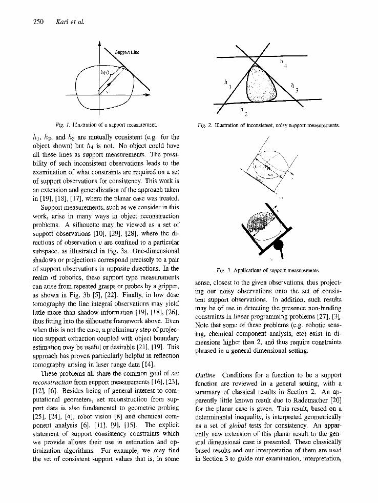
Fig. 1. Illustration of a support measurement.

hi, h2, and ha are mutually consistent (e.g. for the object shown) but h4 is not. No object could have all these lines as support measurements. The possibility of such inconsistent observations leads to the examination of what constraints are required on a set of support observations for consistency. This work is an extension and generalization of the approach taken in [191, [18], [17], where the planar case was treated.

Support measurements, such as we consider in this work, arise in many ways in object reconstruction problems. A silhouette may be viewed as a set of support observations ]10], [29], [28], where the directions of observation v are confined to a particular subspace, as illustrated in Fig. 3a. One-dimensional shadows or projections correspond precisely to a pair of support observations in opposite directions. In the realm of robotics, these support type measurements can arise from repeated grasps or probes by a gripper, as shown in Fig. 3b [5], [22]. Finally, in low dose tomography the line integral observations may yield little more than shadow information [191, [18], [26], thus fitting into the silhouette framework above. Even when this is not the case, a preliminary step of projec- tion support extraction coupled with object boundary estimation may be useful or desirable [21], [19]. This approach has proven particularly helpful in reflection tomography arising in laser range data [14].

These problems all share the common goal of set reconstruction from support measurements [16], [23], [12], [6]. Besides being of general interest to computational geometers, set reconstruction from support data is also fundamental to geometric probing [25], [24], [4], robot vision [8] and chemical component analysis [6], [11], [9], [15]. The explicit statement of support consistency constraints which we provide allows their use in estimation and optimization algorithms. For example, we may find the set of consistent support values that is, in some

Fig. 2. Illuslxation of inconsistent, noisy support measurements.

Fig. 3. Applications of support measurements.

sense, closest to the given observations, thus project- ing our noisy observations onto the set of consistent support observations. In addition, such results may be of use in detecting the presence non-binding constraints in linear programming problems [27], [3]. Note that some of these problems (e.g. robotic sensing, chemical component analysis, etc) exist in dimensions higher than 2, and thus require constraints phrased in a general dimensional setting.

Outline Conditions for a function to be a support function are reviewed in a general setting, with a summary of classical results in Section 2. An apparently little known result due to Rademacher [20] for the planar case is given. This result, based on a determinantal inequality, is interpreted geometrically as a set of global tests for consistency. An apparently new extension of this planar result to the general dimensional case is presented. These classically based results and our interpretation of them are used in Section 3 to guide our examination, interpretation,

Local Tests for Consistency 251

and treatment of the conditions for discrete support sample consistency. Such sampling appears because of the inherently discrete nature of support measurements in applications. Local tests for the consistency of such a set of support samples in arbitrary dimensions are provided. These tests are simple linear inequality tests and are thus simple to perform. In this framework, the local nature of the test is reflected in a banded structure of a corresponding matrix-vector inequality, yielding an efficient test. In what follows, when we refer to a test as being "local" or "global" we will be refering to the nature of the directions involved in the test (i.e. whether they are near to one another or not, respectively).

2. Support Functions: The Continuous Case

2.1. Characterization of Support Functions

The support function H(v) of a set, as defined in (1), is a scalar function of the vector v and hence a map from R ~ to R. A natural question is which functions H(v) could be support functions. Indeed, the problem is classical and the answer is provided by the following result, again classical:

THEOREM 1 (SUPPORT FUNCTION CONDITIONS) A function H(v) is the support function of a convex object if and only if it is defined for all vectors v and has the following properties: 1. H(O) = O. 2. H(c~v) = c~H(v) for a > O. 3. g ( v + w) < H(v) + H(w), Vv, w < .R n.

A proof was given by Minkowski for the 3- dimensional case with other refinements and gener- alizations provided by Rademacher and others (see e.g. [2]). Thus, only positively homogeneous, convex functions are support functions and vice versa. It is condition 3 of subadditivity that is the interesting one, as will be seen later. Note that these conditions are global, in the sense that they must hold for all vectors v and w and thus combine values of the support function over its entire range and not simply values near each other in some sense.

Note that the support function H(v) is easily obtained from the reduced support function h(v) due to the positive homogeneity of H(v) (H(),v) = ),H(v) for A > 0). In fact, the support function H(v) is com-

pletely determined by its values on the unit sphere I]vll = 1, and thus by the function h(v). In particular, for v ¢ O, H(v) = [Ivll h(v/l]vl]), so that if u is a unit vector H(u) = h(u). As a result, conditions on the support function are actually often phrased in terms of the more physically based reduced support function, an approach we will take in what follows. If a valid reduced support function can be found then it may easily be extended to yield a corresponding (full) support function.

For example, in the planar case, a differential condition in terms of h(v) is often used in place of Theo- rem 3. Since in the planar case h(v) is only a function of the direction of v we may parameterize h(v) by the polar angle 0 of v. A twice differentiable function h(O) of 0 is then a (reduced) support function if and only if hoo(O) + h(O) > 0, where hoo(O) is the second derivative of h(O) with respect to 0. Note that this differential condition is a local constraint, in the sense each test only involves properties of the function at the point 0. In particular, hoo(O) + h(O) is equal to the reciprocal of the curvature of the object and for a fixed 0 this is a locally defined quantity. In Theorem 4 we will provide a similar such local result for the discrete case in arbitrary dimensions. Finally, note that Theorem 1 is more fundamental than the commonly used planar differential inequality in that it does not require differentiability of h(O).

Determinantal Condition for the Planar Case Rademacher has shown that it is possible in the planar case to replace the subadditivity condition 3 of The- orem 1 by a determinantal condition on h(u) over unit vectors u. In particular, he showed that under conditions 1 and 2 of Theorem 1, condition 3 holds if and only if

h(u2) u T 1 u T >0 (3)

for all unit vectors ul, u2, and u3, where [ , ] denotes the determinate of the argument [2], [20]. Note that there is no requirement on the differentiability of h(u). Thus we now have a condition directly in terms of the physically measured quantity h(u). This condition is of interest for its geometric interpretation. Assume that ul , u2, and u3 are distinct and that Ua is in the positive or negative cone of {Ul, uz} (which may always be done for three vectors in the plane

252 Karl et aL

u 2

- ~ h ( u 3 )

r I

9

Fig. 4. Illustration of 2-dimensional determinantal condition.

through relabeling). Using a determinantal equality (see Appendix A.1) (3) may then be rewritten as

1E ) h(u2) ] - h(ua) > 0 (4)

where fl(Ul, u2, ua) is a scalar that depends on the u~. In particular, if u3 is in the positive cone of {ul, u2} then /3(ul,u2,ua) > 0 and if u3 is in the negative cone of {ul,u2} then /3(ul,u2,u3) < 0 The term in parentheses in (4), which we call p, is the signed distance along the direction u3 from the support line with normal u3 to the intersection point of the support lines with normals ul and u2, as shown in Fig. 4 for the positive cone case.

In the plane then, the determinantal condition (3), and thus condition 3 of Theorem 1, requires that support functions satisfy an intuitive notion of consistency (as illustrated in Fig. 2 or 4) for all triples of values of the function. This intuition provides a fun- damentally geometric condition for a function to be a support function in the plane, but it is still a global condition, in the sense that all possible combinations of samples must be checked, not just ones near each other.

Higher Dimensions We now turn our attention to finding an equivalent of the geometrically inter- pretable determinantal inequality condition (3) for the higher dimensional case. Unfortunately, in three and higher dimensions the exactly analogous condition (i.e. validity of such a determinant inequality for all vectors u0 has been shown by Rademacher to be satisfied only by the support functions of balls [20]. We identify the difficulty in directly extending this result

x w

I1

u

(a) (b)

Fig. 5. Difference between 2- and 3-dimensional situation.

\ ' , /

T /!,,, f / I 1 ',

F/g. 6. Illustration of 3-dimensional determinantal condition.

and present a natural generalization of condition (3) that is valid for all dimensions. The result appears to be new.

The difference between the two and higher dimensional cases is that in the plane, given three vectors, one of the vectors is always in the positive or negative cone of the remaining two, as shown in Fig. 5a where w is in the positive cone of u and v. In higher dimensions this is not necessarily true, as illustrated by the combination of normals in Fig. 5b. If we consider the geometric interpretation of the test, it seems reasonable to suppose that by restricting our attention to groups of vectors for which this cone condition is satisfied, we might obtain the desired result. This is precisely what we do, yielding the following resuk which is proved in Appendix A.2:

THEOREM 2 (GENERAL INEQUALITY CONDI-

TION) A function H(v) is a support function if and only if it is defined for all v and has the following properties: r . H(O) = O. 2'. H(av) = a l l ( v ) for a > O.


3q The following determinantal inequality is satisfied for all (n + 1)-tuples of unit vectors ui with one in the full positive cone of the others:

:

7" 21,n.+- 1

1 1 u T

i 1 un+ 1

_> o (5)

Recall that for unit vectors u, H(u) = h(u). In a finite dimensional space a cone is said to be full if it cannot be contained in a proper subspace (the im- plication being that the set {ui} is independent). As before, there is no requirement on the differentiability of h(u). Note that the condition requires testing of only positive cone n-tuples. This is a refinement of Rademacher's result for the planar case• It is easy to also include tests of negative cone n-tuples in Theo- rem 2, since this simply adds additional tests which are not really needed.

Now let us interpret this test. Assume un+l is in the positive cone of the remaining {u~}. By using Lemma 2 of Appendix A. 1, we may rewrite (5) as

T U n + l

- 1 uT

¥ U n

h( l) h(u )

- h(un+l) >_ 0 (6)

Similar to the planar case, the left hand side may be naturally interpreted as the signed distance p, positive in the direction of un+l, from the support hyperplane with normal un+l to the point determined by the intersection of the hyperplanes with normals given by u~, i = 1 , . . . , n , as shown for the n = 3 case in Fig. 6.

Condition 3' of our Theorem 2 thus generalizes the intuition of the planar case to arbitrary dimensions. As in the planar case, this condition is still a global one, in the sense that all (n + 1)-tuples of vectors satisfying a positive cone condition must be checked, not just nearby ones. In the following sections we use the intuitions obtained in the continuous case to develop conditions that characterize the consistency of a given set of support samples. An equivalent local result is given in Theorem 4, where only (n + 1)- tuples that are neighbors (defined in an appropriate way) need be checked for consistency.

3. Consistency of Support Samples

In the previous section, we dealt with continuous support functions defined for all directions. The main condition for validity of a support function is a consistency check (the analytic condition 3' of Theo- rem 2) on all positive cone (n + 1)-tuples. In this section the discrete case arising from the sampling of a support function is treated. Due to the presence of noise, a group of such discrete observations will not, in general, be consistent, i.e. there might be no object that could have all the observations as support measurements. An example of such a situation was given in Fig• 2. To be precise, we term a set of support samples consistent if there exists a valid support function whose values at the sample points match the given values. Thus we have the problem of determining when there exists a valid support function h(u) (equivalently H(u)) such that H(ui) = h(ui) = hi for a given a set of m samples {hi} in (unit) directions {ui}.

One obvious approach we could take to identifying inconsistency is to attempt to explicitly find offending hyperplanes, such as h4 in Fig. 2. Essentially what we are doing when we say that h4 is the "inconsistent" sample is implicitly intersecting the directed halfspaces provided by the (hi, ui) pairs to obtain a convex polyhedral region and then attempting to identify those hyperplanes that do not contribute to this region, i.e. that are active constraints. This problem is equivalent to finding the non-binding constraints in a linear programming (LP) problem. This task is com- putationally expensive, essentially necessitating the solution of a dual LP problem itself (details may be found in [1], [27]). Further, it is not really desirable. Such an approach assumes that all the error resides in the inconsistent support measurements, such as h4 of the figure, while the rest are perfect• From an estimation theoretic perspective, the corresponding noise model does not seem reasonable. It is more realistic to assume that all the measurements are corrupted. Hence we instead develop tests or constraints which simply tell of the existence of inconsistency• These constraints essentially serve to define the set of all consistent support samples for a given fixed set of measurement directions ui. This set will in fact be seen to define a polygonal cone in the space of support samples• We are then free to use the conditions as a constraint in the reconstruction of a consistent

254 Karl et al.

set as we see fit. For example, one could use these conditions to project onto the consistent support set.

Our first result shows that a set of samples is consistent if and only if a certain geometric condition (essentially each sample hyperplane being an active constraint in the set definition) is satisfied for all (n + 1)- tuples of sample normals. We then show that under a certain set of assumptions (non-emptiness of intersection) we need only check the (n+ 1)-tuples satisfying a positive cone condition. For such (n + 1)-tuples the geometric condition is identical to the analytic determinantal condition (3 t of Theorem 2) of the continuous case. Finally, under our assumption of nonempty intersection, we do not even require consistency of all these positive cone (n + 1)-tuples, but rather a particular subset corresponding to a natural notion of the (n + 1)-tuples being local to or neighbors of each other.

3.1. Identifying Consistency

First we present a general test for consistency of a set of support samples. This result states that a set of support samples is (globally) consistent (i.e., there is a valid support function which agrees with all the samples) if and only if every (n + 1)-tuple of the set is consistent.

THEOREM 3 (DISCRETE CONSISTENCY) A set of

support samples hi with associated (unit) direction vectors ui is consistent if and only if every (n + 1)- tuple of samples satisfies the following geometric condition:

For every Sample in the (n + 1)-tuple the hyperplane corresponding to the sample has nonempty intersection with the resulting in- (7) tersection of all the corresponding (n + 1) halfspaces.

Theorem 3 is proved using Helly's theorem in Ap- pendix A.3. Now consider the condition (7). For any (n + 1)-tuple with associated unit direction vectors u~, one of the following situations must hold: 1) one ui is in the positive cone of the others, 2) one ui is in the negative cone of the others, or 3) none of the u~ is in the positive or negative cone of the others. We will term (n + 1)-tuples in class 1) positive cone (n + 1)-tuples and those in class 2) neg-

ative cone (n + 1)-tuples. The (n + 1)-tuples in class 3) (neither positive or negative cone) always satisfy condition (7), and therefore are really unimportant in determining consistency. In addition, if we assume that the intersection of all the support sample halfspaces corresponding to the (hi, ui) pairs is nonempty (a gross type of consistency, since it is clearly a necessary condition for the consistency of samples of nontrivial support functions), then the (n + 1)-tuples in class 2) comprising the negative cone tests also satisfy condition (7). Thus, under a nonempty intersection assumption, it is actually sufficient to check the condition (7) for just the (n + 1)-tuples satisfying 1 ) - - i.e., the positive cone tests.

Now, if in such a positive cone (n + 1)-tuple the cone is full (i.e. nondegenerate), then the geometrical condition (7) is equivalent to our determinantal one (5). This can be seen by considering the geometrical interpretation of the condition (5) provided through Lemma 2 and comparing it to (7). Thus these conditions are interchangeable for full positive-cone tests (actually this equivalence is true for full negative- cone tests also, though we will not use this fact in what follows since we will assume nonempty intersection instead). We use these insights to obtain the following corollary to Theorem 3 involving the determinantal condition (5).

COROLLARY i (POSITIVE CONE CONSISTENCY) Given a set of support samples hi with associated (unit) direction vectors u~ in R n, assume that the intersection of all the support sample halfspaces is nonempty and assume that for every positive cone (n + 1)-tuple of sample directions the cone is full. The set of samples is then consistent if and only if condition 3 ~ of Theorem 2 is satisfied by the samples of the set, i.e. if and only if(5) or (7) is satisfied for every positive cone (n ÷ 1)-tuple of the set.

We actually believe that both the assumptions of the corollary are not truly essential. In particular, we believe the first assumption of nonemptiness may actually be replaced by some type of sampling rate constraint, i.e. that if we sample the support function densely enough the satisfaction of the positive cone tests will imply satisfaction of the negative cone tests. Indeed, precisely such a requirement was used in obtaining a similar result for the planar case in [18], [19]. As it stands, the negative cone tests ev- idently just assure nonemptiness, and under dense


3 u 1 U

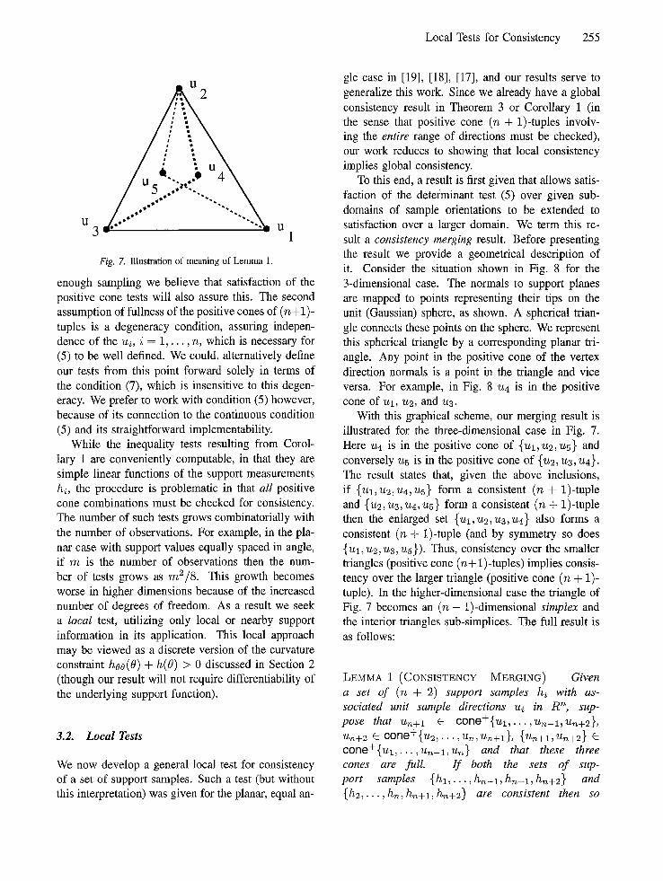
Fig. 7. Illustration of meaning of Lemma 1.

enough sampling we believe that satisfaction of the positive cone tests will also assure this. The second assumption of fullness of the positive cones of (n+l) - tuples is a degeneracy condition, assuring indepen- dence of the ui, i = 1 , . . . ,n, which is necessary for (5) to be well defined. We could, alternatively define our tests from this point forward solely in terms of the condition (7), which is insensitive to this degeneracy. We prefer to work with condition (5) however, because of its connection to the continuous condition (5) and its straightforward implementability.

While the inequality tests resulting from Corol- lary 1 are conveniently computable, in that they are simple linear functions of the support measurements hi, the procedure is problematic in that all positive cone combinations must be checked for consistency. The number of such tests grows combinatorially with the number of observations. For example, in the planar case with support values equally spaced in angle, if m is the number of observations then the number of tests grows as m2/8. This growth becomes worse in higher dimensions because of the increased number of degrees of freedom. As a result we seek a local test, utilizing only local or nearby support information in its application. This local approach may be viewed as a discrete version of the curvature constraint hoo(O) + h(O) > 0 discussed in Section 2 (though our result will not require differentiability of the underlying support function).

3.2. Local Tests

We now develop a general local test for consistency of a set of support samples. Such a test (but without this interpretation) was given for the planar, equal an-

gle case in [19], [181, [17], and our results serve to generalize this work. Since we already have a global consistency result in Theorem 3 or Corollary 1 (in the sense that positive cone (n + 1)-tuples involving the entire range of directions must be checked), our work reduces to showing that local consistency implies global consistency.

To this end, a result is first given that allows satisfaction of the determinant test (5) over given sub- domains of sample orientations to be extended to satisfaction over a larger domain. We term this result a consistency merging result. Before presenting the result we provide a geometrical description of it. Consider the situation shown in Fig. 8 for the 3-dimensional case. The normals to support planes are mapped to points representing their tips on the unit (Gaussian) sphere, as shown. A spherical triangle connects these points on the sphere. We represent this spherical triangle by a corresponding planar triangle. Any point in the positive cone of the vertex direction normals is a point in the triangle and vice versa. For example, in Fig. 8 u4 is in the positive cone of Ul, u2, and u3.

With this graphical scheme, our merging result is illustrated for the three-dimensional case in Fig. 7. Here u4 is in the positive cone of {ul, u2, us} and conversely us is in the positive cone of {u2, u3, u4}. The result states that, given the above inclusions, if {Ul, U2, U4, U5} form a consistent (n + 1)-tuple and {u2, u3, u4, us} form a consistent (n + 1)-tuple then the enlarged set {Ul,UZ,U3,U4} also forms a consistent (n + 1)-tuple (and by symmetry so does {Ul, u2, u3, us}). Thus, consistency over the smaller triangles (positive cone (n+ 1)-tuples) implies consistency over the larger triangle (positive cone (n + 1)- tuple). In the higher-dimensional case the triangle of Fig. 7 becomes an (n - 1)-dimensional simplex and the interior triangles sub-simplices. The full result is as follows:

LEMMa 1 (CoNsISTENCY MERGINC) Given a set of (n + 2) support samples hi with associated unit sample directions ui in R n, suppose that u~+l E cone+{u t , . . . , u~- l ,Un+2} , Un+2 C cone+{u2,..., us, u~+l}, {u,+l, u,+2} c cone+{u l , . . . ,u ,~_ l ,u ,~} and that these three cones are full. I f both the sets of support samples { h l , . . . , h n - l , h ~ + l , h n + 2 } and { h 2 , . . . , h m h~+l, h~+2} are consistent then so

256 Karl et al.

S> J

U U 3

Fig. 8. Graphical representation scheme for normal relationships.

\ I ~ ~ S SS

Fig. 9. Illustration of a local family

are the enlarged sets { h l , . . . , h n , h~+l} and {hi, • • •, h~, h~+2}.

In the above, cone + denotes the positive cone of a set and by consistency of a set we mean satisfaction of the determinantal inequality (5) or, equivalently, the condition (7) by the set. The proof of this result is in Appendix A.4.

A suitable notion of "local" now needs to be defined for the general case, or, in the context of Lemma 1, we need to know the minimal domain over which consistency must be satisfied. For the planar case, as studied in [19], [18], [17], this notion of locality is straightforward, depending on normal order- ing and adjacency. In higher dimensions, however, the situation is not so clear. Adjacent faces do not necessarily correspond to nearest normals anymore. A natural notion of locality is suggested both by condition 3 ~ of Theorem 2 and by Lemma 1 with their emphasis on a positive cone condition on the unit sample normals. Given a sample normal, we define what we mean to be "local" to that sample normal in the following:

DEFINITION 1 (LOCAL FAMILY) Given a set ,.~ of m distinct unit vectors in R r~ and a member from this

set Uk, we define the local family corresponding to uk to be the set of all distinct (n + 1)-tuples of vectors from S such that uk is one element of the (n + 1)- tuple and the remaining n vectors of the ( n + 1)-tuple contain only themselves and uk from S in their full positive cone.

Thus, the local family corresponding to the element uk is a set of (n+ 1)-tuples, each containing uk and with the property that the only nontrivial element of the parent set contained in the positive cone of the remaining n-tuple is the generating element uk. In terms of the paradigm of Fig. 8, a local family is defined by the set of all (spherical) triangles (simplices in higher dimensions) containing the given normal ue but no others, as shown in Fig. 9 for the n = 3 case. In contrast to the planar case, where there is just a single local neighbor, this notion of locality implies a family of tests associated to each normal, one for each (n + 1)-tuple in the corresponding local family.

Local Constraint With these ideas of locality defined we are prepared to present our main result showing that local consistency and global consistency are equivalent.

THEOREM 4 (LOCAL CONSISTENCY 4==~ GLOBAL CONSISTENCY) Given a set of support samples hi with associated (unit) direction vectors ui in R n, assume that the intersection of all the support sample halfspaces is nonempty and assume that for every positive cone (n + 1)-tuple of sample directions the cone is full. Then the overall set of samples is consistent if and only if for each sample normal uk, all elements of the corresponding local family are consistent.

In other words, the overall set is consistent if and only if all elements of all local families are consistent.


lo'

~ 10 3

i ~1o ~

9

"5

~c lO ~

lO ~ lO ~ Number of randomly chosen directions

Fig. 10. Example of computational savings of a local verses global test as the number of uniformly chosen sample directions is increased in R a.

Again, consistency of a (n + 1)-tuple means satisfaction of (5) or (equivalently) (7). Thus, we have that a set is globally consistent if and only if it is locally consistent, where locality is defined in the sense of the local family of a sample normal. The proof of the result is in Appendix A.5.

Note that each of the tests (5) required in Theo- rem 4 is linear in the support samples hi. As a result, given a set of m samples and t such tests (where t is the total number tests to be performed), we may write the corresponding set of tests as

Oh > 0 (8)

where h = [hi, h2. . . , hm] T is the vector of support samples (termed the support vector), Q is a t x m sparse matrix guaranteed to have only n + 1 non-zero entries in each row, and 0 is a t vector of zeros. Since the definition of the local families depends only on the sample normals ui and not on the support samples themselves, the matrix Q also depends only on the normals ui. Consequently, once these directions are fixed the matrix Q may be precomputed and then applied to many different sets of measurements. Note, since the inequality constraints are linear and finite, the set of all consistent support samples is defined by a polygonal cone in the m-dimensional space of support samples with fixed direction.

This form of constraint is particularly convenient for constrained support reconstruction. For example, suppose that we are given a set of noisy support observations in the vector y taken in corresponding known directions ui and that we wish to reconstruct

the least square error estimate of h from these observations subject to consistency. The resulting problem combines (8) with a least squares criteria to yield the following linear inequality constrained least squares problem, which is straightforward to solve:

la =arg rain [Ih - YI[2 (9) Oh_>O

This model of known u~ but noisy h~ is reasonable for many problems, particularly medical and non- destructive evaluation tomography problems, where the user may exercise great control over the geometry of the data acquisition. The situation is obviously more complicated if we consider the, perhaps more realistic, situation of noisy measurements h~ coupled with imperfectly known geometry ui. Such situations arise in geophysical problems and target tracking [14], [13].

In general, obtaining a complete, general complex- ity analysis of the advantage of using our local test over the standard exhaustive one appears to be a dif- ficult (but interesting) combinatorial problem. Some things are apparent however. For example, let us consider the case where we choose M directions randomly and uniformly in R k. First consider the be- havior around a fixed set of directions. It is straightforward to show that the number of (global) positive cone tests involving each fixed sample of this set is Q ( M k) on average 1. Since we may choose the number of elements in this set as a fixed fraction cM of the total number of directions, the overall number of positive cone tests should be Q(Mk+l ) .

On the other hand, if we choose a fixed local positive cone test (k + 1)-tuple and now start selecting M randomly and uniformly drawn directions, the probability that this fixed local (k + 1)-tuple remains a local test goes to zero exponentially fast 2 as a function of M. Note, that at the same time this fixed (k + 1)-tuple will always be a (global) positive cone test regardless of how many new directions are added. The above arguments suggest that the number of local tests will be much smaller than the total number of positive cone tests, particularly for high dimensions k and large numbers of samples M. Note that since we would expect each of the M directions to be involved in at least one local test, we expect the number of local tests to be at least @(M), and so the ratio of total to local tests to be at most (~)(Mk).

258 Karl et al.

i

i hi " ' .

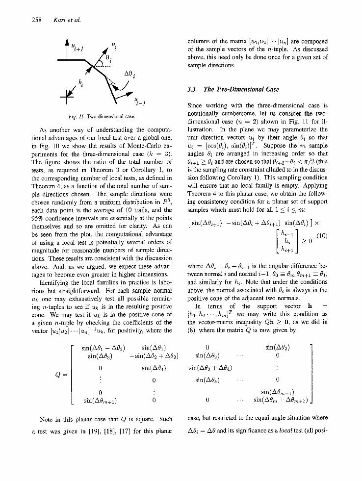
Fig. 11. Two-dimensional case.

As another way of understanding the computational advantages of our local test over a global one, in Fig. 10 we show the results of Monte-Carlo ex- periments for the three-dimensional case (k = 3). The figure shows the ratio of the total number of tests, as required in Theorem 3 or Corollary 1, to the corresponding number of local tests, as defined in Theorem 4, as a function of the total number of sample directions chosen. The sample directions were chosen randomly from a uniform distribution in R a, each data point is the average of 10 trails, and the 95% confidence intervals are essentially at the points themselves and so are omitted for clarity. As can be seen from the plot, the computational advantage of using a local test is potentially several orders of magnitude for reasonable numbers of sample directions. These results are consistent with the discussion above. And, as we argued, we expect these advantages to become even greater in higher dimensions.

Identifying the local families in practice is labo- rious but straightforward. For each sample normal uk one may exhaustively test all possible remaining n-tuples to see if uk is in the resulting positive cone. We may test if uk is in the positive cone of a given n-tuple by checking the coefficients of the vector [UllUZ[... lu~l-luk, for positivity, where the

Q =

columns of the matrix Julius[ . . . lun] are composed of the sample vectors of the n-tuple. As discussed above, this need only be done once for a given set of sample directions.

3.3. The Two-Dimensional Case

Since working with the three-dimensional case is notationally cumbersome, let us consider the two- dimensional case (n = 2) shown in Fig. 11 for illustration. In the plane we may parameterize the unit direction vectors ui by their angle Oi so that ui = [cos(0i), sin(0i)] r . Suppose the m sample angles 0~ are arranged in increasing order so that 0i+1 _> 0i and are chosen so that Oi+2-Oi < 7r/2 (this is the sampling rate constraint alluded to in the discussion following Corollary 1). This sampling condition will ensure that no local family is empty. Applying Theorem 4 to this planar case, we obtain the following consistency condition for a planar set of support samples which must hold for all 1 < i < m:

[ sin(AO/+l) -- sin(A0i q- mOiq_l) sin(A0i) ] x

1] 0

where AOi = Oi - Oi-1 is the angular difference between normal i and normal / -1 , 0o -- Om 0rn+l ~ 01, and similarly for hi. Note that under the conditions above, the normal associated with 0i is always in the positive cone of the adjacent two normals.

In terms of the support vector h = [hi, h 2 . . . , kin] T we may write this condition as the vector-matrix inequality Qh _> 0, as we did in (8), where the matrix Q is now given by:

- sin(A01 + A02) sin(A01) 0 sin(A02) sin(A03) - sin(A02 + A03) sin(A02) . . . 0

0 sin(A04) - sin(A03 + A04) :

: 0 sin(A05) . . . 0

0 : sin(A0m-1) sin(A0m+a) 0 0 . . . . sin(A0m + A0m+l)

Note in this planar case that Q is square. Such

a test was given in [19], [18], [17] for this planar

case, but restricted to the equal-angle situation where

AOi = A0 and its significance as a local test (all posi-


five cone 4-tuples are not tested) was not brought out. The planar test (10) for non-uniformly spaced angles may also be found in [14].

Note that these types of tests do not identify which constraints are inconsistent. To see this, consider the situation shown in Fig. 13, where the intersections of the adjacent support lines used in the local tests are shown as the points Pi and the object is assumed contained in the darker, shaded region at the bottom. The support measurements with normals u2, u3, u4, would fail the local test at point P2, since the line associated with u3 is behind P2 (in the direction given by ua). While this failure does confirm the existence of inconsistency, note that the set of samples associated with ul, u2, and u3, would pass their local test at PI• The distance from the u2 support line to Pl is positive in the direction given by u~ so the local test is satisfied. Thus, while the sample with normal u2 is also inconsistent, it is not identified by the local tests.

4. Conclusions

In this work we have presented a unified and general treatment of the consistency requirements for both a support function and a set of support samples corresponding to a fixed set of directions• We extended a classical determinantal condition for the existence and uniqueness of a support function and then used the resulting insights to develop a general dimensional inequality test for consistency of a set of support samples• We subsequently developed a local test for sample consistency, in the sense that each inequality only involved local support information. Such a result may be viewed as the general dimensional, discrete equivalent of the well known planar support curvature constraint.

Appendix

A.1. Derivation of Geometric Lemma

In this appendix we prove a result we repeatedly use, and which we state as the lemma:

LEMMA 2 Suppose the unit vectors {ui}, i = 1 , . . : , n are independent and that the unit vector un+i is in the (full) positive or negative cone of the

set {ui}, i = 1 , . . . , n. Then the following equality

holds for some 13(ul , . . . ,un+l), with/3 > 0 / f un+l is in the positive cone and/3 < 0 i f un+l is in the negative cone, and fl = 0 i f and only i f Un+ l = u~ for some i = 1 , . . . , n:

(Ul)

:

H(Un+l) T %tn+l

- 1

uT

Un-}-i

H( I) H(u2)

(A1)

- H ( u ~ + l ) )

Note that if the ui are not independent the determinantal condition is trivially zero and our expression is not well defined since the matrix of the ui is not invertible. Also, note that if one of the u~ is in a cone formed by the others and it happens not to be un+l, we need only interchange rows and relabel. Such operations do not change the sign of the result because the row exchanges will take place in both the determinant terms on the left hand side of (A1).

Proof" First note that since un+i is in the cone formed by the set {u~}, i = 1 , . . . , n, we may write it as the following linear combination:

U n - k l : [Ull... lUn] O~ 1

OZ n

(A2)

with cti _> 0 for the positive cone case and c~i _< 0 for the negative cone case•

Now apply the following determinantal identity to each term of the left hand side of (A1):

A B C D -- I A I I D - CA-1BI

Doing this to the first term yields:

H(u.+~) T Un+l

= (-i?

uT

U n

H(ul)

H(u )

260 Karl et aL

= ( - -1 ) n + l X U l(IU L "~n

-1 [ H(ul) H( 2)

H(un)

- H(Un+l))

Similarly applying the determinantal identity to the second term yields for it:

u2 T

i '//'n + 1

( - -1 ) n + l U T U T 1 • unT+I . . - 1

j i Now combining the two expressions and equating terms with the expression on the right hand side of the lemma shows that the scalar/3 is given by: [Ul ]l[1] /

u T U~+l u~ 1 /3

~Z n U n

= (-1) n+J u~ 1. u~•

:r 1 T Us "U'n+ 1

(A3)

Substituting the expression (A2) for ui+l into the second term shows that it is equal to ( ~ = 1 a i - 1) thus:

fl(ttl~•..~Un-F1 ) = u T n 1

• O ~ i - -

¥

(A4)

To show/3 is of the appropriate sign, let us separately consider the two cases of U~+l contained in the positive or negative cone of the remaining ui. Note that the first term of/3 in (A4) is clearly positive for either case, since the ui, i = 1 , . . . , n are independent (they form a full cone) by assumption.

Case 1: Pos i t ive c~i > 0, for each uTuj _< 1 for all

1 ----IlUn+lll 2 =

Cone For this case we have that i. Since u~+l is a unit vector and i, j we have:

n

i=1 j=l

i=1 j = l

Since o~i _> 0 this implies that ~ c~ > 1 so that the second term in (A4) is nonnegative. This shows that

/3_>0. n Now from (A4)/3 = 0 if and only if Y~i=l c~i = 1.

From (A5) this implies that/3 = 0 if and only if:

n

i=l j=l i=1 j=l (A6)

Each term on the left hand side of (A6) is less than or equal to the corresponding term on the right hand side. In particular, equality for a term is achieved if and only if either uTuj = 1 or c~iaj = 0. Since u~uj < 1 if i ¢ j , we can have equality in (A6) (equivalently,/3 = 0) if and only if

a i a j = 0, Vi, j , i ¢ j (A7)

Since ~-~n = ~=1 c~i = 1 this can only be if c~i 1 for some i and c~j = 0 for all j such that j 7~ i, so that Un+l = ui for s o m e i = 1 , . . . , n . Thus /3 = 0 i f and only if un+l = ui for some i = 1 , . . . ,n , and the positive cone case is shown•

For a more geometrical understanding of the case when fl = 0, note that the condition that ~i=in c~i = 1 coupled with (A2) implies that/3 = 0 if and only if


un+l is in the hyperplane defined by { u l , . . . , un} (we can also arrive at this conclusion by considering that/3 = 0 implies that the last term in (A3) is identically zero, which can only be if all the vectors { u l , . . . , u = + l } lie in a hyperplane). Since the ui are unit vectors, this hyperplane intersects the unit spheroid in an (n - 1)-dimensional hypersphere containing the vectors {Ul , . . . , un} , as shown by the circle through ul, u2, and ua for the 3-dimensional case in Fig. A.1. Now since u~+l itself is a unit vector, it must lie somewhere in this intersection hypersphere. The only points on this intersection hypersphere that are also in the positive cone of the {u l , - . . ,un} (denoted by the triangle in Fig. A.1) are the ui themselves.

Case 2: Negative Cone For this case we have that a,; < 0, for each i. From (A4) clearly /3 < 0.

A.2. Proof of Theorem 2

Proof. To prove the result we need only show that condition 3' of Theorem 2 implies and is implied by condition 3 of Theorem 3. First, we show that condition 3 implies 3 ~. Consider an arbitrary (n + 1)-tuple of unit dh'ection vectors ui with Un+t in the positive cone of the remaining vectors. If Un_bl = U i for any i = 1 , . . . , n then 3' of Theorem 2 is trivially satisfied. Suppose such is not the case. Using Lemma 2 of Appendix A. 1 together with the fact that we may write u,~+l as in (A2) we obtain:

H(Ul) H( 2)

H(Un+l)

u T 1 u T

u T 1 U T

u T 1 T n+l Un+l

= /3 a~H(ui - H o~,ui (A8)

H(a iu i ) - H a~u~ [.i=1

with ~ ( U l , . . . , u ~ + J > 0. Now by the subadditivity condition 3 of Theorem 3, H(o~z i + O~jUj) <

H ( c q u 0 + H ( a j u j ) for any a~, a j , u~, uj, It follows that:

H(a ui) - H a ui >_ 0 i=1

(A9)

Thus (A8) must be nonnegative. Since the vectors u~ of the positive cone (n + 1)-tuple were arbitrary this shows that condition 3 implies condition 3 ~.

Now we show that condition 3 ~ implies condition 3. Given arbitrary vectors v and w, we will show that if 3' is satisfied then H ( v + w ) < H ( v ) + H ( w ) .

If v is a scalar multiple of w this is trivially true from condition 2 or 2q Assume such is not the case. In condition 3' let Ul = v/[]v[[, u2 = w/[[wI[ and choose the remaining ui, i = 3 , . . . , n arbitrarily to span the subspace perpendicular to v and w. Let u ,+l = ( v + w ) / l l v + w l l , so that un+~ is a unit vector in the full positive cone of the ui. In particular, we have that:

0 .

Now by assumption condition 3 ~ is satisfied and, using Lemma 2, it follows that:

T ~n+l

- 1

- >_ 0

for any n + 1 unit vectors ui, with u~+l in the positive cone of the remaining ones but not equal to any of them. Substituting the expressions above for ul, u2, and Un+l we obtain

Ilvll Ilwll 11~+~oll

;r ? ~n ~n

0 . . . O ] x - -1

H<, H (It@t)

- H I1 +

262 Karl et al.

_ . ) Equivalently, using condition 2,

1 IIv + wll (H(v) + H(w) - H(v + w)) > O.

Thus

H(v + w) < H(v) + H(w)

and the converse is shown. Together these implica- tions prove the result. •


Proof" To prove Theorem 3 we will make use of the following well known theorem:

T H E O R E M 5 ( H E L L Y ' S T H E O R E M ) A collection of convex sets in R ~ has nonempty intersection if and only if every collection of n + 1 sets at a time has nonempty intersection•

Given a set of m support samples one can always form a polyhedron (which may possibly be empty) by intersecting the m half-spaces corresponding to the support samples• Call this polyhedron P. That global consistency of a support sample set implies satisfaction of the condition (7) for every (n + 1)-tuple (i.e. local consistency) is obvious. To show the other direction, we need to show that if every (n + 1)-tuple of samples satisfies the condition (7), then there exists a valid support function agreeing with the samples or, equivalently, that the intersection of the hyperplane corresponding to each sample with the polygon P is nonempty.

To this end, suppose that every (n + 1)-tuple of samples satisfies the condition (7) (i.e. is locally consistent) and consider the i-th sample• We need to show that the hyperplane corresponding to this sample has nonempty intersection with P. The hyperplane corresponding to the i-th sample consists of the intersection of two halfspaces. The intersection of this hyperplane with P thus consists of the intersection of m + 1 halfspaces - - 2 for the hyperplane of the i-th sample and m - 1 for the halfspaces of the other m - 1 samples. Since by assumption every (n + 1)- tuple of samples satisfies (7), it follows that the intersection of every (n + 1)-tuple of these halfspaces is nonempty. Hence, by Helly's theorem it follows that

the intersection of all m + 1 halfspaces is nonempty, so that the i-th hyperplane has nonempty intersection with P. Since this is true for each i -- 1 , . . . , m, the m samples are (globally) consistent, with the support function of P giving one valid support function.

A.4. Proof of Lemma 1

Proof" We show that under the hypotheses of the lemma the enlarged set { h l , . . . , h~, h~+l} is consistent. Consistency of the set {ha , . . . , h~,h~+2} then follows by symmetry. We know that %n+l C (30r' le+{ul , . . .~Un-l ,Un+2} and Un+2 E cone+{u2,..., U n , U n + l } , thus we may write Un+l and u~+2 as the following linear combinations:

U n + l =

U . . . U n ]

~2

+ an+2Un+2 (A10)

Un+ 2 =

721 • . . U n ]

0 62

63 + 6 n + l U n + l

6n

(All)

where 0 _< ~x~ and 0 < 6i. Note that an and 61 are 0. We may eliminate un+2 from the above two expressions to obtain the following equivalent expression for Un+l :

1 Un] ×

Ztn+ 1 ---- j. - - 6n+ lO~n+ 2 U •. • U2 Un--1

O11

0~2 + 6201n+2

Otn--1 + 6 n - - l O / n + 2

6nO/.n+2

(A12)

This expression provides the representation of Un+l with respect to the cone defined by {Ul, . . . ,Un}.


Since Un+l is in the full positive cone of these direction vectors by assumption and this representation is unique, the coefficients of the ui, i = 1 , . . . , n in the expansion (A12) must be nonnegative and finite. In particular, since c~i and ~i, i = 1 , . . . , n + 2 are nonnegative and not all zero, we must have that (1 - c~+1c~+2) > 0.

Now consistency of the set {hi , . • •, h~_ 1, hn+ 1, h~+2 } implies through (5) and Lemma 2 that the following inequality is satisfied:

hi h2

%T n+l [U l U2 . . Un--1 Un-k2 ] - T

h~-z hn+2

- hn+l >_ 0

Substitution of (A10) for U~+l into this inequality and rearrangement yields

[ch c~2 . . . a ~ - i 0 - 1 a n + 2 ] h > 0 (A13)

where ,3 is a nonnegative scalar depending on the Ul,.. . , Un+ 1. We may equivalently write this as

p = /~ (Ul : . . . : %r~+ 1) X

1 - ~ n + l ~ n + 2 / -

a l 0 ~ 2 ~2

~ 3 h T a _ + a~+2 i

11 ~ n

~ n + l \ . ~ n + 2 . - 1

which will be recognized as a linear combination of the left hand sides of (A13) and (A14). Now the terms/3/(1 - ~nA_lOZn_F2) and a,~+2 are nonnegative so (A16) is equal to a nonnegative linear combination of (A13) and (A14), which are also nonnegative. Consequently, (A16) and thus (A15) must also be nonnegative and we have demonstrated consistency of the set { h i , . . . , hn, hn+l}. The lemma is thus shown. •

where h = [hi,h2,. . . , hn+2] T is termed the support vector. Similarly, consistency of the set {h2, . . . , h~, hn+l, hn+2} together with (All) yields the following inequality, through use of (5) and Lemma 2:

[ 0 0 L 20L 3 " '" ~n ~ n + l - 1 ] h _> 0 (A14)

Thus, (A13) and (A14) are true by assumption. To show consistency of the samples

{h l , . . . , hmh~+l} we have to show that the following expression is nonnegative

hi ul T 1 u T h2 u T 1 u T

(A15) P = : : : :

hn+l T 1 U T U n + l n + l

Applying Lemma 2 again and substituting for u,~+l from (A12) shows that the expression (A15) is equivalent to:

D = /~ ( l t l ' " " " ' ~n-t-1) [OZl ' (0~2 -F (5~20~n-k2), 1 -- OZn+lOLn+ 2

(O!3 -4- (~30~n+2), ' ' " , (OLn--1 -F (SZn--lOZn+2),

~,~ct~+2, (~+lC~n+2 - 1), 0] h (A16)


Proof." That global consistency implies local consistency follows easily, for if a set is globally consistent then by definition the inequality (5) is satisfied for all unit vectors in the full positive cone of an n-tuple of other sample normals.

Thus, we need to show that local sample consistency implies global sample consistency. First note that under the assumptions of the result, global consistency is assured if (5) or (7) are satisfied for every positive cone (n + 1)-tuple due to Corollary 1. Now let us assume that the (n + 1)-tuples corresponding to the local families are consistent and show how this implies that any positive cone (n + 1)-tuple will then be consistent. To this end, consider an arbitrary support sample hj and its associated unit direction normal u j, in the positive cone of some (possibility non-local) n-tuple of other sample normals, i.e. an arbitrary positive cone (n + 1)-tuple. On the surface of the n-dimensional unit (Gaussian) spheroid the unit direction vector uj (in the positive cone of the n other unit vectors) is a point inside an (n - 1)-dimensional spherical simplex (generalization of a spherical triangle), as described in association with Fig. 8 for the

264 Karl et aL

3-dimensional case. Points in this simplex are points in the positive cone of the vectors at the vertices of the simplex, as is u4 in Fig. 8

/ 3 "~'>>.1>,x Pl I/]lllll/llllll~~

Fig. 13. Illustration of non-specificity of local tests.

Fig, A,1. Illustration of 2-dimensional intersection.

U 1 . ~ U q ~ J

U l ~ . u j / u 3 ~ u °

~ U l k uj ~ 1 ~ u2 ' Uk

i u

2

Fig. 12. Illustration of geometry

If the point associated with uj is isolated in the

simplex it is consistent by hypothesis, since it is the only vector in the positive cone of the normal directions at the vertex, and hence part of a local family.

Suppose instead that there is another point in the simplex with it, say uk as shown in the leftmost illustration of Fig. 12 for the 3-dimensional case. Each of these two interior points (corresponding to direction vectors uj and uk) in combination with the n original bounding points (corresponding to an n-tuple of direction vectors) tessellates the original simplex into

on unit (Gaussian) sphere.

n disjoint subsimplicies whose union is the original simplex• The two interior points corresponding to uj and uk are thus each contained in a subsimplex formed from the other interior point and n - 1 of the original boundary points. This geometry is shown in the leftmost frame of Fig. 12 as two dotted triangles.

Now by the merging result, Lemma 1, if we can show that the samples u3 and uk are consistent on these smaller subregions then we have shown that they are consistent on the entire region, as desired. Thus we have reduced the problem from showing consistency over the original region to showing con-


sistency over two smaller subregions. This process is shown in the middle illustration of the figure, where we h a v e spl i t the o r ig ina l tes t in to two subtests . We

m a y n o w repea t the a b o v e a rgumen t s on each of the

subregions, attempting to show the consistency of each. We thus have the following finitely terminating recursive construction:

Show an arbitrary positive c o n e ( n + 1 ) - t u p l e is consistent: 1. If it is isolated in its cone, consistency is shown

by hypothesis. 2. If it is not isolated:

(a) Pick another point in the cone.

(b) Form two smaller subregions.

(c) A~empt to show consistency of each subregion.

We keep proceeding in this way until a subregion is found where the interior point is isolated (corresponding to the normal being the only vector in the positive cone of its bounding set) and consistency is satisfied by hypothesis. In Fig. 12 we show the next step of th is p r o c e d u r e on the r ight , whe re we h a v e a s s u m e d

that the subregion containing uj is isolated (so that we have reached a leaf of the tree) but the one containing u~ contains another point, Uq and hence must itself be broken into two subregions.

Since at each stage of this procedure another point (sample normal) is removed from the original finite set and since the subregions are nonincreasing at each stage, we must eventually reach the situation where a sample normal is isolated in its simplex and therefore cons is ten t . U s i n g L e m m a 1 we m ay then t ravel

b a c k up the t ree we h a v e impl ic i t ly c rea ted to show

c o n s i s t e n c y o f the o r ig ina l s a m p l e wi th respec t to the

or ig ina l b o u n d a r y points . S ince the or ig ina l pos i t ive-

cone ( n + 1) - tup le we chose was arbitrary, we have

s h o w n the result .

Notes

1. To see this pick k fixed area patches forming a simplex containing the chosen direction. Every combination of points from these patches forms a positive cone test involving the fixed direction. The expected fraction of the M total points in each patch is proportional to the area fraction "7 of each patch, which is a constant. Since there are k patches, the expected number of tests involving the fixed direction will go as 7 k M k, which is ©(Mk).

2. To see this, note that the test will remain local only if no other sample directions appear in the chosen, fixed simplex. Now the probability p of a sample direction being in the simplex is just the area fraction of the simplex, which is fixed. Thus the probability of the test being local after M directions are chosen is just (1 - p ) M , which goes to zero exponentially fast.

References

1. H. C. R Berbee, C. G. E. Boender, A. H. G. Rinnooy Kan, C. L. Scheffer, R. L. Smith, and J. Telgen. Hit-and-run algorithms for the identification of nonredundant linear inequalities. Mathematical Programming, 37:184-207, 1987.

2. T. Bonnesen and W. Fenchel. Theory of Convex Bodies. BCS Associates, Moscow, Idaho, 1987.

3. M.C. Cheng. General criteria for rendundant and nonredan- dant linear inequalities. Journal of Optimization Theory and Applications, 53(1):37-42, April 1986.

4. H. Edelsbrunner and S. S. Skiena. Probing convex polygons with X-rays. SIAM J. Computing, 17(5):870-882, October 1988.

5. R C. Gaston and R. Lozano-Perez. Tactile recognition and localization using object models: The case of polyhedra on the plane. IEEE Journal of Pattern Analysis and Machine Intelligence, 6(3):257-266, 1984.

6. J. R Greschak. Reconstructing Convex Sets. PhD thesis, Massachusetts Institute of Technology, February 1985.

7. H. Guggenheimer. Applicable Geometry: Global and Local Convexity. Applied Mathematics Series. Krieger, Hunting- ton, New York, 1977.

8. B.K. R Horn. Robot Vision. MIT Press, Cambridge, 1986. 9. J.M. Humel. Resolving bilinear data arrays. Master's thesis,

Massachusetts Institute of Technology, 1986. 10. W. C. Karl and G. C. Verghese. Curvatures of surfaces and

their shadows. Linear Algebra and its Applications, 130:231- 255, 1990.

11. R.R. Kim. Matrix Algorithms for Bilinear Estimation Prob- lems in Chemometrics. PhD thesis, Massachusetts Institute of Technology, June 1985.

12. D.T. Lee and E E Preparata. Computational geometry - - a survey. IEEE Transactions on Computers, C-33:1072-1101, 1984.

13. A.S. Lele. Convex set reconstruction from support line measurements and its application to laser radar data. Master's thesis, Massachusetts Institute of Technology, April 1990.

14. A. S. Lele, S. R. Kulkarni, and A. S. Willsky. Convex- polygon estimation from support-line measurements and applications to target reconstruction from laser-radar data. Jour- nal of the Optical Society of America A, 9(10):1693-1714, October 1992.

266 Karl et al.

15. N. Ohm. Estimating absorption bands of component dyes by means of principal component analysis. Anal. Chem., 45:553-557, 1973.

16. E P. Preparata and M. I. Shamos. Computational Geometry: An Introduction. Springer-Verlag, Paris, 3rd edition, 1990.

17. J. L. Prince. Geometric Model-based Estimation from Pro- jections. PhD thesis, Massachusetts Institute of Technology, January 1988.

18. J. L, Prince and A. S, WiUsky. Reconstructing convex sets from support line measurements. IEEE Journal of Pattern Analysis and Machine Intelligence, 12(4):377-389, April 1990.

19. J. L. Prince and A. S. Willsky. Convex set reconstruction using prior shape information. CVGIP: Graphical Models and Image Processing, 53(5):413427, September 1991.

20. H. Rademacher. /3ber eine fnnktionale ungleichung in der theorie der konvexen kSrper. Mathematische ~ Zeitschrift, 13:18-27, 1922.

21. D. J. Rossi and A. S. Willsky. Reconstruction from projections based on detection and estimation of objects - parts I and II: Performance analysis and robustness analysis. 1EEE Transactions on Acoustic, Speech, and Signal Processing, ASSP-32(4):886-906, 1984.

22. J.L. Schneiter and T. B. Sheridan. An automated tactile sensing strategy for planar object recognition and localization. IEEE Journal of Pattern Analysis and Machine Intelligence, 12(8):775-786, August 1990.

23. M. I. Shamos. Computational Geometry. PhD thesis, Yale University, December 1977.

24. S. S. Skiena. Problems in geometric probing. Algorithmica, 4:599-605, 1989.

25. S. S. Skiena. Probing convex polygons with half-planes. Journal of Algorithms, 12(3):359-374, September 1991.

26. H. Stark and H. Peng. Shape estimation in computer tomography from minimal data. In E. S. Gelsema and L. N. Kanal, editors, Pattern Recognition and Artificial Intelligence: To- wards and Integration, volume 7 of Machine Intelligence and Pattern Recognition, pages 185-200. North-Holland, Ams- terdam, 1988.

27. J. Telgen. Redundancy and Linear Programs. Mathematisch Centmm, Amsterdam, 1981.

28. P. Van Hove and J. Verly. A silhouette slice theorem for opaque 3-D objects. In International Conference on Acous- tic and Speech Signal Processing, pages 933-936, March 1985.

29. P.L. Van Hove. Silhouette-Slice Theorems. PhD thesis, Mas- sachusetts Institute of Technology, Department of Electrical Engineering and Computer Science, September 1986.

William C. Karl received the Ph.D. degree in Electrical Engineering and Computer Science in 1991 from the Mas- sachusetts Institute of Technology, Cambridge, where he also received the S.M., E.E., and S.B. degrees. He held the position of Staff Research Scientist with the Brown- Harvard-M.I.T. Center for Intelligent Control Systems and the M.I.T. Laboratory for Information and Decision Sys- tems from 1992 to 1994. He joined the faculty of Boston University in January 1995, where he is currently Assis- tant Professor of Electrical, Computer, and Systems Engi- neering, In 1993 Dr, Karl was organizer and chair of the "Geometry and Estimation" session of the Conference on Information Sciences and Systems at Johns Hopkins Uni- versity. In 1994 he was on the technical committee for the Workshop on Wavelets in Medicine and Biology, part of the International Conference of the IEEE Engineering in Medicine and Biology Society. Dr. Karl's research interests are in the areas of multidimensional and multiscale signal and image processing and estimation, particularly applied to geometrically and medically oriented problems.

Sanjeev Kulkarni received the B.S. in Mathematics, B.S. in E.E., M.S. in Mathematics from Clarkson University in 1983, 1984, and 1985, respectively, the M.S. degree in E.E. from Stanford University in 1985, and the Ph.D. in E.E. from M.I.T. in 1991.


From 1985 to 1991 he was a Member of the Technical Staff at M.I.T. Lincoln Laboratory working on the mod- eling and processing of laser radar measurements. In the spring of 1986, he was as a part-time faculty at the Uni- versity of Massachusetts, Boston. Since 1991, he has been an Assistant Professor of Electrical Engineering at Prince- ton University. He received an ARO Young Investigator Award in 1992 and an NSF Young Investigator Award in 1994. His research interests include pattern recognition, nonparametric estimation, statistical inference, and image processing.

George C. Verghese received his B. Tech, from the In- dian Institute of Technology at Madras in 1974, his M.S. from the State University of New York at Stony Brook in 1975, and his Ph.D. from Stanford University in 1979, all in electrical engineering.

He is Professor of Electrical Engineering and a member of the Laboratory for Electromagnetic and Electronic Sys- tems at the Massachusetts Institute of Technology, which he joined in 1979. His research interests and publications are in the areas of systems, control, and estimation, especially as applied to power electronics, electrical machines, large power systems, and signal processing.

Dr. Verghese has served as an Associate Editor of Auto- matica and of the IEEE Transactions on Automatic Control. He is co-author (with J.G. Kassakian and M.E Schlecht) of Principles of Power Electronics, Addison-Wesley, 1991.

ogy in 1969 and 1973 respectively. He joined the M.I.T. faculty in 1973 and his present position is Professor of Elec- trical Engineering. From 1974 to 1981 Dr. Willsky served as Assistant Director of the M.I.T. Laboratory for Informa- tion and Decision Systems. He is also a founder and member of the board of directors of Alphatech, Inc. In 1975 he received the Donald E Eckman Award from the American Automatic Control Council. Dr. Willsky has held visit- ing positions at Imperial College, London, L'Universite de Paris-Sud, and the Institut de Recherche en Informatique et Systemes Aleatoires in Rennes, France. He was p'rbgram chairman for the 17th IEEE Conference on Decision and Control, has been an associate editor of several journals including the IEEE Transactions on Automatic Control, has served as a member of the Board of Governors and Vice President for Technical Affairs of the IEEE Control Sys- tems Society, was program chairman for the 1981 Bilateral Seminar on Control Systems held in the People's Republic of China, and was special guest editor of the 1992 special issue of the IEEE Transactions on Information Theory on wavelet transforms and multiresolution signal analysis. Also in 1988 he was made a Distinguished Member of the IEEE Control Systems Society. In addition Dr. Willsky has given several plenary lectures at major scientific meetings including the 20th IEEE Conference on Decision and Con- trol, the 1991 IEEE International Conference on Systems Engineering, the SIAM Conf. on Control 1992, 1992 In- augural Workshop for the National Centre for Robust and Adaptive Systems, Canberra, Australia, and the IEEE Sym- posium on Image and Multidimensional Signal Processing in Cannes, France in 1993.

Dr. Willsky is the author of the research monograph Digital Signal Processing and Control and Estimation The- ory and is co-author of the undergraduate text Signals and Systems. He was awarded the 1979 Alfred Noble Prize by the ASCE and the I980 Browder J. Thompson Memorial Prize Award by the IEEE for a paper excerpted from his monograph. Dr. Willsky's research interests are in the de- velopment and application of advanced methods of estimation and statistical signal and image processing. Methods he has developed have been successfully applied in a wide variety of applications including failure detection in high- performance aircraft, advanced surveillance and tracking

cardiogram analysis, computerized tomog- ~te sensing.

Alan S, Willsky received both the S.B. degree and the Ph.D. degree from the Massachusetts Institute of Technol-

Documents

Local Tests for Consistency of Support Hyperplane Datassg.mit.edu/~willsky/publ_pdfs/133_pub_MIV.pdf · Local Tests for Consistency of Support Hyperplane Data WILLIAM C. KARL* wckarl