Embed Size (px)
Citation preview

ESL 4.4.3-4.5 Logistic Regression (contd.) & Separating Hyperplane
June 8, 2015 Talk by Shinichi TAMURA
Mathematical Informatics Lab @ NAIST
Today's topics ¨ Logistic regression (contd.)"
¨ On the analogy with Least Squares Fitting"¨ Logistic regression vs. LDA"
¨ Separating Hyperplane"¨ Rosenblatt's Perceptron"¨ Optimal Hyperplane"
Today's topics ¨ Logistic regression (contd.)"
¨ On the analogy with Least Squares Fitting"¨ Logistic regression vs. LDA"
¨ Separating Hyperplane"¨ Rosenblatt's Perceptron"¨ Optimal Hyperplane"

Today's topics ¨ Logistic regression (contd.)"
¨ On the analogy with Least Squares Fitting"¨ Logistic regression vs. LDA"
¨ Separating Hyperplane"¨ Rosenblatt's Perceptron"¨ Optimal Hyperplane"

Today's topics ¨ Logistic regression (contd.)"
¨ On the analogy with Least Squares Fitting"¨ Logistic regression vs. LDA"
¨ Separating Hyperplane"¨ Rosenblatt's Perceptron"¨ Optimal Hyperplane"
On the analogy with Least Squares Fitting
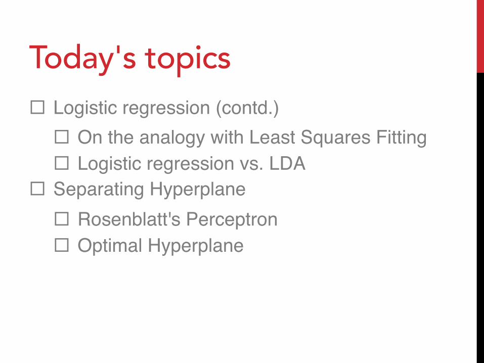
[Review] Fitting LR Model Parameters are fitted by ML estimation, using Newton-Raphson algorithm:""""
!new !rgmin!
(z " X!)#W(z " X!)
!new =(X#WX)"1X#Wz.

On the analogy with Least Squares Fitting
[Review] Fitting LR Model Parameters are fitted by ML estimation, using Newton-Raphson algorithm:""""It looks like least squares fitting:"
!new !rgmin!
(z " X!)#W(z " X!)
!new =(X#WX)"1X#Wz.
!!rgmin!
(y " X!)#(y " X!)
! =(X#X)"1X#y
On the analogy with Least Squares Fitting
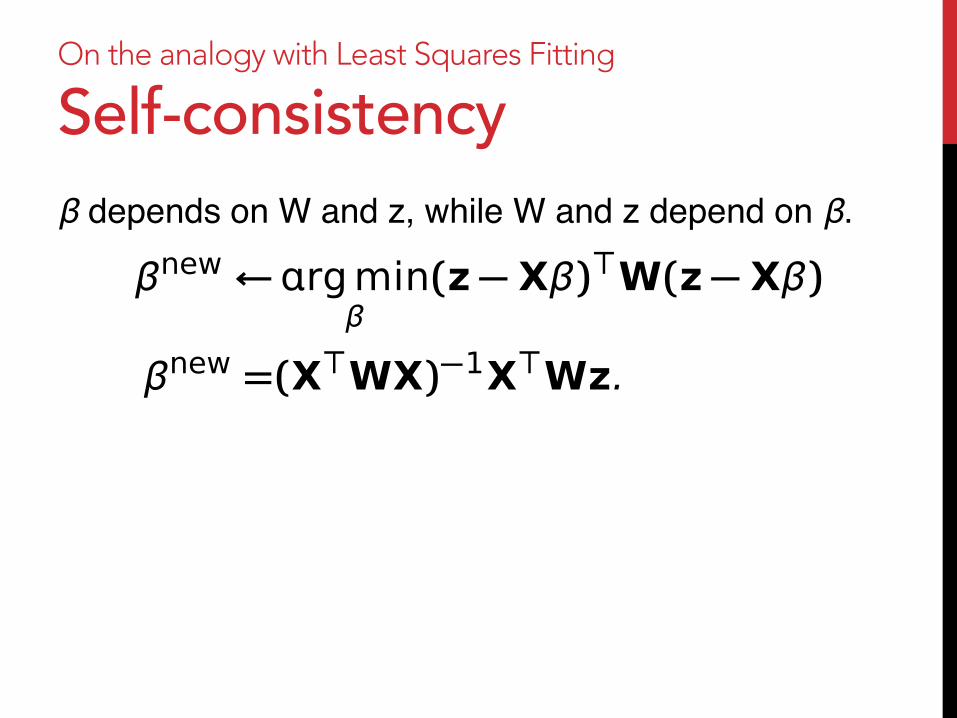
Self-consistency β depends on W and z, while W and z depend on β.""""""
!new !rgmin!
(z " X!)#W(z " X!)
!new =(X#WX)"1X#Wz.
On the analogy with Least Squares Fitting
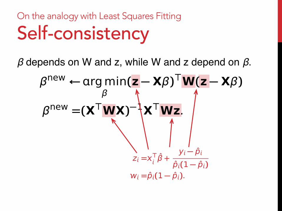
Self-consistency β depends on W and z, while W and z depend on β.""""""
!new !rgmin!
(z " X!)#W(z " X!)
!new =(X#WX)"1X#Wz.
z =! β̂ +y " p̂
p̂(1 " p̂) =p̂(1 " p̂).

On the analogy with Least Squares Fitting
Self-consistency β depends on W and z, while W and z depend on β."""""→ “self-consistent” equation, needs iterative method
to solve""
!new !rgmin!
(z " X!)#W(z " X!)
!new =(X#WX)"1X#Wz.

On the analogy with Least Squares Fitting
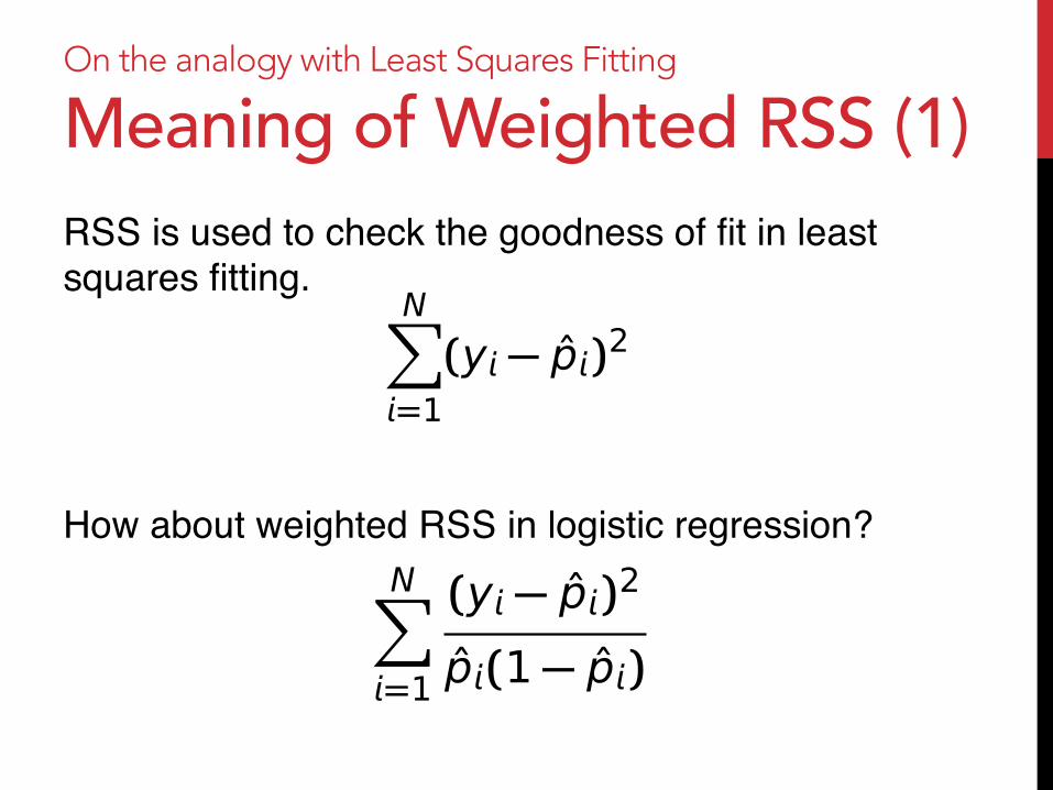
Meaning of Weighted RSS (1) RSS is used to check the goodness of fit in least squares fitting."""
N!
=1(y ! p̂)2
On the analogy with Least Squares Fitting
Meaning of Weighted RSS (1) RSS is used to check the goodness of fit in least squares fitting.""""How about weighted RSS in logistic regression?"
N!
=1(y ! p̂)2
N!
=1
(y ! p̂)2
p̂(1 ! p̂)

On the analogy with Least Squares Fitting
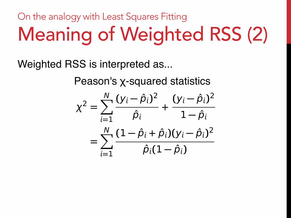
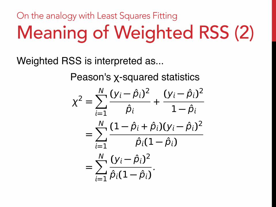
Meaning of Weighted RSS (2) Weighted RSS is interpreted as..."
Peason's χ-squared statistics"
χ2 =N!
=1
(y ! p̂)2
p̂+(y ! p̂)2
1 ! p̂
=N!
=1
(1 ! p̂ + p̂)(y ! p̂)2
p̂(1 ! p̂)
=N!
=1
(y ! p̂)2
p̂(1 ! p̂).
On the analogy with Least Squares Fitting
Meaning of Weighted RSS (2) Weighted RSS is interpreted as..."
Peason's χ-squared statistics"
χ2 =N!
=1
(y ! p̂)2
p̂+(y ! p̂)2
1 ! p̂
=N!
=1
(1 ! p̂ + p̂)(y ! p̂)2
p̂(1 ! p̂)
=N!
=1
(y ! p̂)2
p̂(1 ! p̂).
On the analogy with Least Squares Fitting
Meaning of Weighted RSS (2) Weighted RSS is interpreted as..."
Peason's χ-squared statistics"
χ2 =N!
=1
(y ! p̂)2
p̂+(y ! p̂)2
1 ! p̂
=N!
=1
(1 ! p̂ + p̂)(y ! p̂)2
p̂(1 ! p̂)
=N!
=1
(y ! p̂)2
p̂(1 ! p̂).

On the analogy with Least Squares Fitting
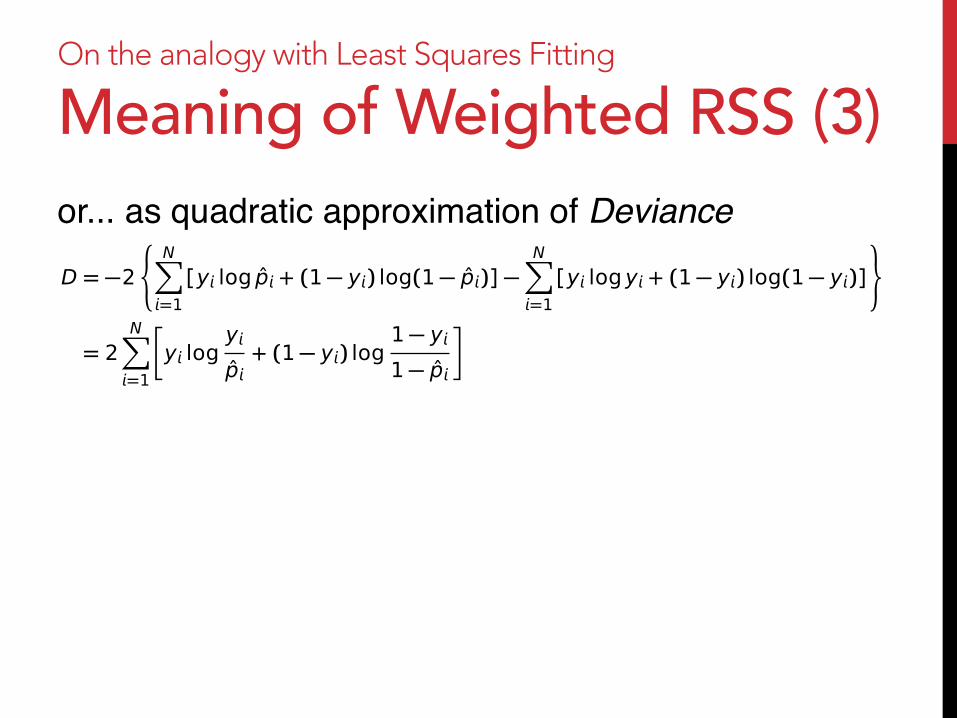
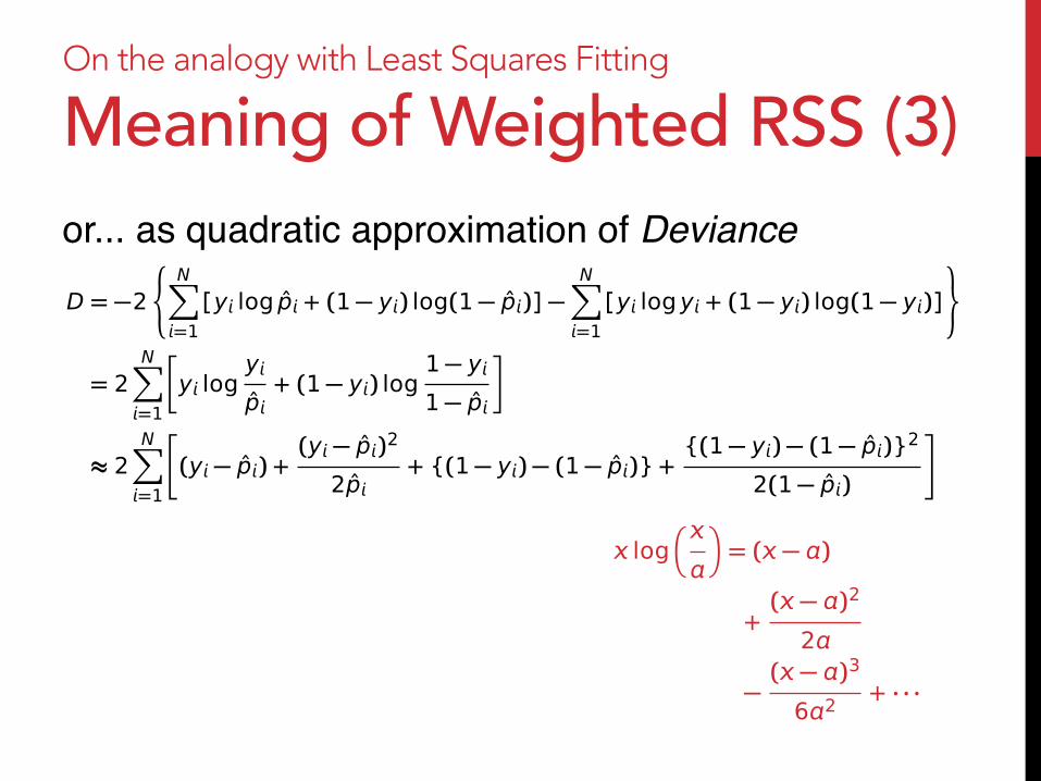
Meaning of Weighted RSS (3) or... as quadratic approximation of Deviance"D = !2!
N"
=1[y log p̂ + (1 ! y) log(1 ! p̂)] !
N"
=1[y logy + (1 ! y) log(1 ! y)]
#
= 2N"
=1
$y log
yp̂+ (1 ! y) log
1 ! y1 ! p̂
%
" 2N"
=1
&(y ! p̂) +
(y ! p̂)2
2p̂+ {(1 ! y) ! (1 ! p̂)} +
{(1 ! y) ! (1 ! p̂)}2
2(1 ! p̂)
'
=N"
=1
(y ! p̂)2
p̂+(y ! p̂)2
1 ! p̂
=N"
=1
(y ! p̂)2
p̂(1 ! p̂).

On the analogy with Least Squares Fitting
Meaning of Weighted RSS (3) or... as quadratic approximation of Deviance"D = !2!
N"
=1[y log p̂ + (1 ! y) log(1 ! p̂)] !
N"
=1[y logy + (1 ! y) log(1 ! y)]
#
= 2N"
=1
$y log
yp̂+ (1 ! y) log
1 ! y1 ! p̂
%
" 2N"
=1
&(y ! p̂) +
(y ! p̂)2
2p̂+ {(1 ! y) ! (1 ! p̂)} +
{(1 ! y) ! (1 ! p̂)}2
2(1 ! p̂)
'
=N"
=1
(y ! p̂)2
p̂+(y ! p̂)2
1 ! p̂
=N"
=1
(y ! p̂)2
p̂(1 ! p̂).
Maximum likelihood of the model
Likelihood of the full model which achieve perfect fitting
On the analogy with Least Squares Fitting
Meaning of Weighted RSS (3) or... as quadratic approximation of Deviance"D = !2!
N"
=1[y log p̂ + (1 ! y) log(1 ! p̂)] !
N"
=1[y logy + (1 ! y) log(1 ! y)]
#
= 2N"
=1
$y log
yp̂+ (1 ! y) log
1 ! y1 ! p̂
%
" 2N"
=1
&(y ! p̂) +
(y ! p̂)2
2p̂+ {(1 ! y) ! (1 ! p̂)} +
{(1 ! y) ! (1 ! p̂)}2
2(1 ! p̂)
'
=N"
=1
(y ! p̂)2
p̂+(y ! p̂)2
1 ! p̂
=N"
=1
(y ! p̂)2
p̂(1 ! p̂).
00
log!
"= ( ! )
+( ! )2
2
!( ! )3
62+ · · ·

On the analogy with Least Squares Fitting
Meaning of Weighted RSS (3) or... as quadratic approximation of Deviance"D = !2!
N"
=1[y log p̂ + (1 ! y) log(1 ! p̂)] !
N"
=1[y logy + (1 ! y) log(1 ! y)]
#
= 2N"
=1
$y log
yp̂+ (1 ! y) log
1 ! y1 ! p̂
%
" 2N"
=1
&(y ! p̂) +
(y ! p̂)2
2p̂+ {(1 ! y) ! (1 ! p̂)} +
{(1 ! y) ! (1 ! p̂)}2
2(1 ! p̂)
'
=N"
=1
(y ! p̂)2
p̂+(y ! p̂)2
1 ! p̂
=N"
=1
(y ! p̂)2
p̂(1 ! p̂).
00

On the analogy with Least Squares Fitting
Meaning of Weighted RSS (3) or... as quadratic approximation of Deviance"D = !2!
N"
=1[y log p̂ + (1 ! y) log(1 ! p̂)] !
N"
=1[y logy + (1 ! y) log(1 ! y)]
#
= 2N"
=1
$y log
yp̂+ (1 ! y) log
1 ! y1 ! p̂
%
" 2N"
=1
&(y ! p̂) +
(y ! p̂)2
2p̂+ {(1 ! y) ! (1 ! p̂)} +
{(1 ! y) ! (1 ! p̂)}2
2(1 ! p̂)
'
=N"
=1
(y ! p̂)2
p̂+(y ! p̂)2
1 ! p̂
=N"
=1
(y ! p̂)2
p̂(1 ! p̂).
On the analogy with Least Squares Fitting
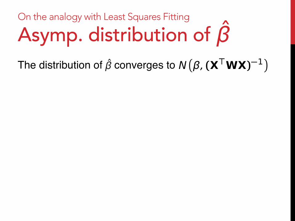
Asymp. distribution of The distribution of converges to "N
!!, (X!WX)"1
"!̂
!̂

On the analogy with Least Squares Fitting
Asymp. distribution of The distribution of converges to "(See hand-out for the details)"
N!!, (X!WX)"1
"
yi.i.d.! Bern(Pr(;β)).
! E[y] = p, vr[y] =W.
! E!β̂"= E!(X"WX)#1X"Wz
"
= (X"WX)#1X"WE!Xβ +W#1(y # p)
"
= (X"WX)#1X"WXβ= β,
vr!β̂"= (X"WX)#1X"Wvr
!Xβ +W#1(y # p)
"W"X(X"WX)#"
= (X"WX)#1X"W(W#1WW#")W"X(X"WX)#"
= (X"WX)#1.
!̂
!̂
On the analogy with Least Squares Fitting
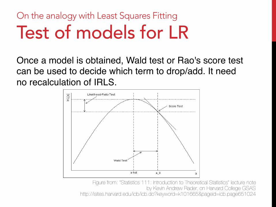
Test of models for LR Once a model is obtained, Wald test or Rao's score test can be used to decide which term to drop/add. It need no recalculation of IRLS."
Figure from: "Statistics 111: Introduction to Theoretical Statistics" lecture note by Kevin Andrew Rader, on Harvard College GSAS
http://isites.harvard.edu/icb/icb.do?keyword=k101665&pageid=icb.page651024
On the analogy with Least Squares Fitting
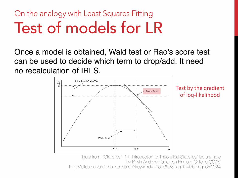
Test of models for LR Once a model is obtained, Wald test or Rao's score test can be used to decide which term to drop/add. It need no recalculation of IRLS."
Figure from: "Statistics 111: Introduction to Theoretical Statistics" lecture note by Kevin Andrew Rader, on Harvard College GSAS
http://isites.harvard.edu/icb/icb.do?keyword=k101665&pageid=icb.page651024
Test by the gradient of log-‐likelihood

On the analogy with Least Squares Fitting
Test of models for LR Once a model is obtained, Wald test or Rao's score test can be used to decide which term to drop/add. It need no recalculation of IRLS."
Figure from: "Statistics 111: Introduction to Theoretical Statistics" lecture note by Kevin Andrew Rader, on Harvard College GSAS
http://isites.harvard.edu/icb/icb.do?keyword=k101665&pageid=icb.page651024
Test by the difference of paremeter
On the analogy with Least Squares Fitting
L1-regularlized LR (1) Just like lasso, L1-regularlizer is effective for LR."

On the analogy with Least Squares Fitting
L1-regularlized LR (1) Just like lasso, L1-regularlizer is effective for LR."Here the objective function will be:"""""
mxβ0,β
!N"
=1logPr(;β0,β) ! λ"β"1
#
=mxβ0,β
!N"
=1
$y(β0 + β#) ! log
%1 + eβ0+β
#&'! λ
p"
j=1|βj|#.

On the analogy with Least Squares Fitting
L1-regularlized LR (1) Just like lasso, L1-regularlizer is effective for LR."Here the objective function will be:"""""The resulting algorithm can be called “iterative reweighted lasso” algorithm."
mxβ0,β
!N"
=1logPr(;β0,β) ! λ"β"1
#
=mxβ0,β
!N"
=1
$y(β0 + β#) ! log
%1 + eβ0+β
#&'! λ
p"
j=1|βj|#.
On the analogy with Least Squares Fitting
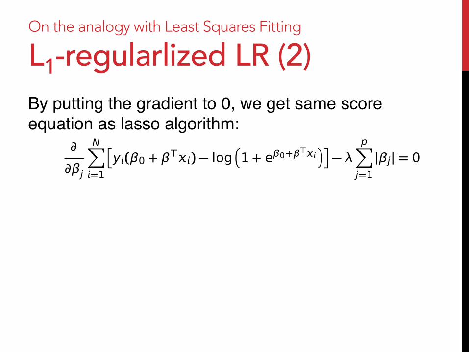
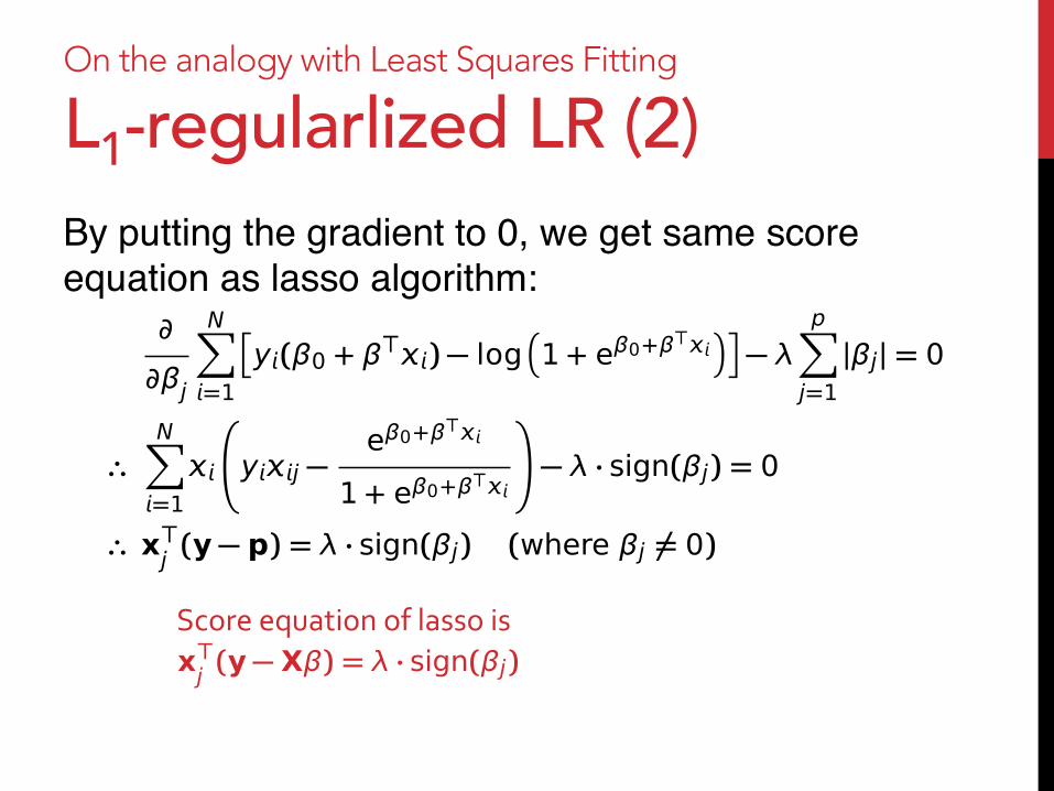
L1-regularlized LR (2) By putting the gradient to 0, we get same score equation as lasso algorithm:"
∂
∂βj
N!
=1
"y(β0 + β!) " log
#1 + eβ0+β
!$%" λ
p!
j=1|βj| = 0
!N!
=1
&yj "
eβ0+β!
1 + eβ0+β!
'" λ · sign(βj) = 0
! x!j (y " p) = λ · sign(βj) (where βj #= 0)00

On the analogy with Least Squares Fitting
L1-regularlized LR (2) By putting the gradient to 0, we get same score equation as lasso algorithm:"
∂
∂βj
N!
=1
"y(β0 + β!) " log
#1 + eβ0+β
!$%" λ
p!
j=1|βj| = 0
!N!
=1
&yj "
eβ0+β!
1 + eβ0+β!
'" λ · sign(βj) = 0
! x!j (y " p) = λ · sign(βj) (where βj #= 0)
00

On the analogy with Least Squares Fitting
L1-regularlized LR (2) By putting the gradient to 0, we get same score equation as lasso algorithm:"
∂
∂βj
N!
=1
"y(β0 + β!) " log
#1 + eβ0+β
!$%" λ
p!
j=1|βj| = 0
!N!
=1
&yj "
eβ0+β!
1 + eβ0+β!
'" λ · sign(βj) = 0
! x!j (y " p) = λ · sign(βj) (where βj #= 0)
x!j (y " X!) = " · sign(!j)Score equation of lasso is
On the analogy with Least Squares Fitting
L1-regularlized LR (3) Since the objective function is concave, the solution can be obtained using optimization techniques.""
On the analogy with Least Squares Fitting
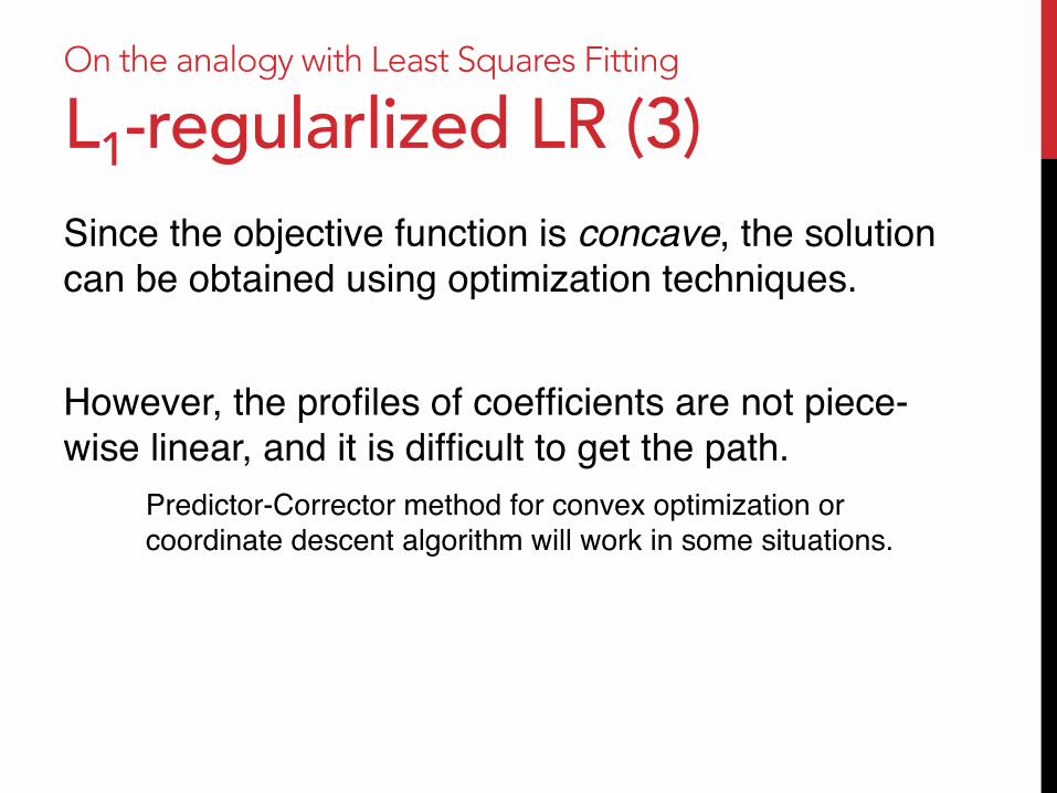
L1-regularlized LR (3) Since the objective function is concave, the solution can be obtained using optimization techniques.""However, the profiles of coefficients are not piece-wise linear, and it is difficult to get the path."
Predictor-Corrector method for convex optimization or coordinate descent algorithm will work in some situations."
On the analogy with Least Squares Fitting
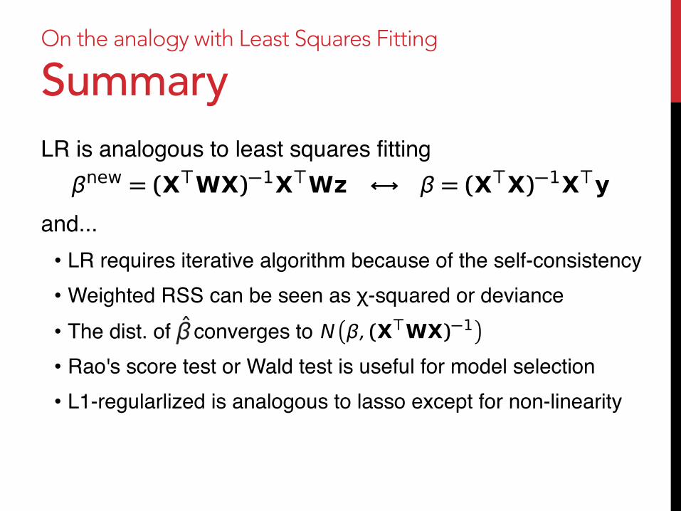
Summary LR is analogous to least squares fitting""and..."• LR requires iterative algorithm because of the self-consistency"• Weighted RSS can be seen as χ-squared or deviance"• The dist. of converges to "• Rao's score test or Wald test is useful for model selection"• L1-regularlized is analogous to lasso except for non-linearity"
!new = (X!WX)"1X!Wz # ! = (X!X)"1X!y
N!!, (X!WX)"1
"!̂
Today's topics ¨ Logistic regression (contd.)"
¨ On the analogy with Least Squares Fitting"¨ Logistic regression vs. LDA"
¨ Separating Hyperplane"¨ Rosenblatt's Perceptron"¨ Optimal Hyperplane"
Today's topics ¨ Logistic regression (contd.)"
þ On the analogy with Least Squares Fitting"¨ Logistic regression vs. LDA"
¨ Separating Hyperplane"¨ Rosenblatt's Perceptron"¨ Optimal Hyperplane"
Logistic regression vs. LDA
What is the different LDA and logistic regression are very similar methods."Let us study the characteristics of these methods through the difference of formal aspects."
Logistic regression vs. LDA
Form of the log-odds """

Logistic regression vs. LDA
Form of the log-odds LDA""""
logPr(G = k|X = )
Pr(G = K |X = )= log
πkπK!1
2(μk + μK)"!1(μk ! μK)
+ "!1(μk ! μK)=αk0 + α"k ,

Logistic regression vs. LDA
Form of the log-odds LDA"""""Logistic regression"
logPr(G = k|X = )
Pr(G = K |X = )= log
πkπK!1
2(μk + μK)"!1(μk ! μK)
+ "!1(μk ! μK)=αk0 + α"k ,
logPr(G = k|X = )
Pr(G = K |X = )=βk0 + β!k .

Logistic regression vs. LDA
Form of the log-odds LDA"""""Logistic regression"
logPr(G = k|X = )
Pr(G = K |X = )= log
πkπK!1
2(μk + μK)"!1(μk ! μK)
+ "!1(μk ! μK)=αk0 + α"k ,
logPr(G = k|X = )
Pr(G = K |X = )=βk0 + β!k .
Same form
Logistic regression vs. LDA
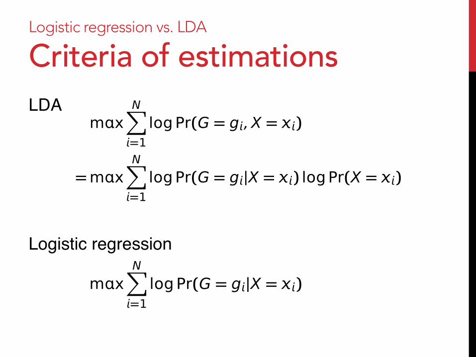
Criteria of estimations ""

Logistic regression vs. LDA
Criteria of estimations LDA"""""
mxN!
=1logPr(G = g, X = )
=mxN!
=1logPr(G = g|X = ) logPr(X = )
Logistic regression vs. LDA
Criteria of estimations LDA"""""Logistic regression"
mxN!
=1logPr(G = g, X = )
=mxN!
=1logPr(G = g|X = ) logPr(X = )
mxN!
=1logPr(G = g|X = )
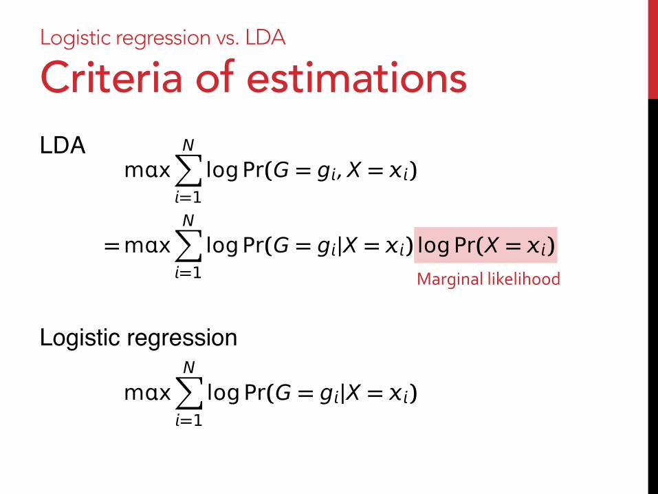
Logistic regression vs. LDA
Criteria of estimations LDA"""""Logistic regression"
mxN!
=1logPr(G = g, X = )
=mxN!
=1logPr(G = g|X = ) logPr(X = )
mxN!
=1logPr(G = g|X = )
Marginal likelihood
Logistic regression vs. LDA
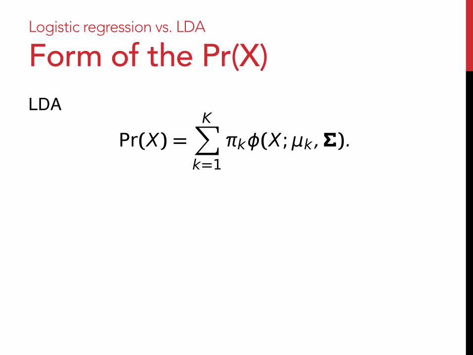
Form of the Pr(X) ""
Logistic regression vs. LDA
Form of the Pr(X) LDA"""
Pr(X) =K!
k=1πkϕ(X;μk,).
Logistic regression vs. LDA
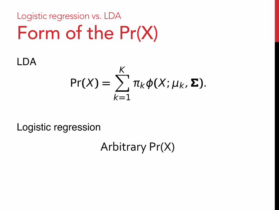
Form of the Pr(X) LDA""""Logistic regression"
Pr(X) =K!
k=1πkϕ(X;μk,).
Arbitrary Pr(X)

Logistic regression vs. LDA
Form of the Pr(X) LDA""""Logistic regression"
Pr(X) =K!
k=1πkϕ(X;μk,).
Arbitrary Pr(X)
Involves parameters

Logistic regression vs. LDA
Effects of the difference (1) How these formal difference affect on the character of the algorithm?"
Logistic regression vs. LDA
Effects of the difference (2) The assumption of Gaussian and homoscedastic can be strong constraint, which lead low variance."

Logistic regression vs. LDA
Effects of the difference (2) The assumption of Gaussian and homoscedastic can be strong constraint, which lead low variance."In addition, LDA has the advantage that it can make use of unlabelled observations; i.e. semi-supervised is available."

Logistic regression vs. LDA
Effects of the difference (2) The assumption of Gaussian and homoscedastic can be strong constraint, which lead low variance."In addition, LDA has the advantage that it can make use of unlabelled observations; i.e. semi-supervised is available.""On the other hand, LDA could be affected by outliers."
Logistic regression vs. LDA
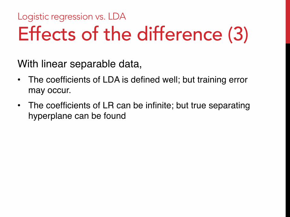
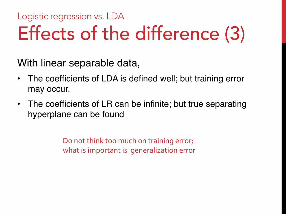
Effects of the difference (3) With linear separable data,"

Logistic regression vs. LDA
Effects of the difference (3) With linear separable data,"• The coefficients of LDA is defined well; but training error
may occur."
Logistic regression vs. LDA
Effects of the difference (3) With linear separable data,"• The coefficients of LDA is defined well; but training error
may occur."• The coefficients of LR can be infinite; but true separating
hyperplane can be found"
Logistic regression vs. LDA
Effects of the difference (3) With linear separable data,"• The coefficients of LDA is defined well; but training error
may occur."• The coefficients of LR can be infinite; but true separating
hyperplane can be found"
Do not think too much on training error; what is important is generalization error

Logistic regression vs. LDA
Effects of the difference (4) The assumptions for LDA rarely hold in practical."

Logistic regression vs. LDA
Effects of the difference (4) The assumptions for LDA rarely hold in practical."
Nevertheless, it is known empirically that these models give quite similar results, even when LDA is used inappropriately, say with qualitative variables."
"

Logistic regression vs. LDA
Effects of the difference (4) The assumptions for LDA rarely hold in practical."
Nevertheless, it is known empirically that these models give quite similar results, even when LDA is used inappropriately, say with qualitative variables."
"After all, however, if Gaussian assumption looks to hold, use LDA. Otherwise, use logistic regression."

Today's topics ¨ Logistic regression (contd.)"
þ On the analogy with Least Squares Fitting"¨ Logistic regression vs. LDA"
¨ Separating Hyperplane"¨ Rosenblatt's Perceptron"¨ Optimal Hyperplane"
Today's topics ¨ Logistic regression (contd.)"
þ On the analogy with Least Squares Fitting"þ Logistic regression vs. LDA"
¨ Separating Hyperplane"¨ Rosenblatt's Perceptron"¨ Optimal Hyperplane"

Today's topics þ Logistic regression (contd.)"
þ On the analogy with Least Squares Fitting"þ Logistic regression vs. LDA"
¨ Separating Hyperplane"¨ Rosenblatt's Perceptron"¨ Optimal Hyperplane"
Separating Hyperplane: Overview Another way of Classification Both LDA and LR do classification through the probabilities using regression models.""

Separating Hyperplane: Overview Another way of Classification Both LDA and LR do classification through the probabilities using regression models.""Classification can be done by more explicit way: modelling the decision boundary directly."

Separating Hyperplane: Overview Properties of vector algebra Let L be the affine set defined by"""
"
"and the signed distance from x to L is "
β0 + β! = 0
d±(, L) =1
!β! (β" + β0)
β0 + β! > 0" is above L
β0 + β! = 0" is on L
β0 + β! < 0" is below L
Today's topics þ Logistic regression (contd.)"
þ On the analogy with Least Squares Fitting"þ Logistic regression vs. LDA"
¨ Separating Hyperplane"¨ Rosenblatt's Perceptron"¨ Optimal Hyperplane"

Today's topics þ Logistic regression (contd.)"
þ On the analogy with Least Squares Fitting"þ Logistic regression vs. LDA"
p Separating Hyperplane"p Rosenblatt's Perceptron"p Optimal Hyperplane"
Rosenblatt's Perceptron
Learning Criteria The basic criteria of Rosenblatt's Perceptron learning algorithm is to reduce (M is misclassified data)"
D(β,β0) =!
!M"# β + β0"
!!
!M"d±(, L)"
= $!
!My(# β + β0)
00

Rosenblatt's Perceptron
Learning Criteria The basic criteria of Rosenblatt's Perceptron learning algorithm is to reduce (M is misclassified data)"
D(β,β0) =!
!M"# β + β0"
!!
!M"d±(, L)"
= $!
!My(# β + β0)
00
Rosenblatt's Perceptron
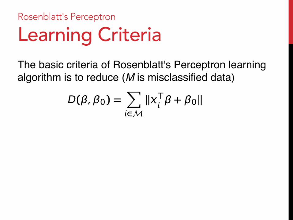
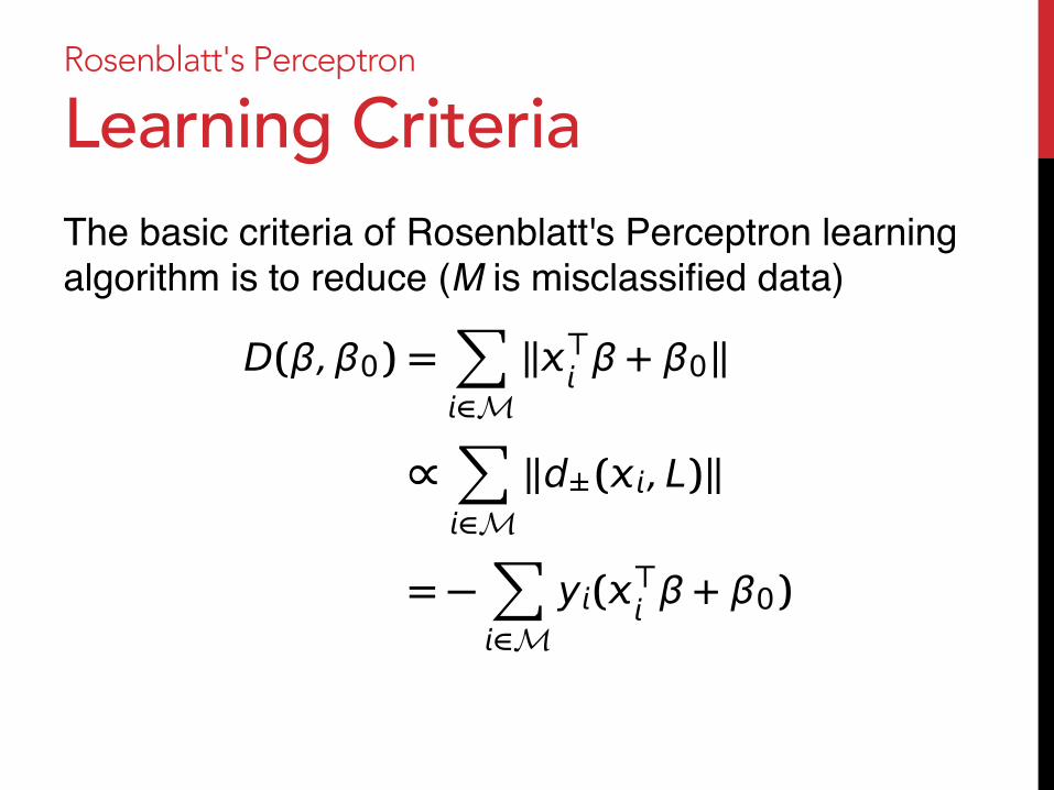
Learning Criteria The basic criteria of Rosenblatt's Perceptron learning algorithm is to reduce (M is misclassified data)"
D(β,β0) =!
!M"# β + β0"
!!
!M"d±(, L)"
= $!
!My(# β + β0)

Rosenblatt's Perceptron
Learning Criteria The basic criteria of Rosenblatt's Perceptron learning algorithm is to reduce (M is misclassified data)"
D(β,β0) =!
!M"# β + β0"
!!
!M"d±(, L)"
= $!
!My(# β + β0)
If misclassified yi=1 as -‐1, the latter part is negative
Rosenblatt's Perceptron
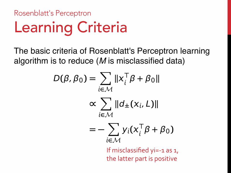
Learning Criteria The basic criteria of Rosenblatt's Perceptron learning algorithm is to reduce (M is misclassified data)"
D(β,β0) =!
!M"# β + β0"
!!
!M"d±(, L)"
= $!
!My(# β + β0)
If misclassified yi=-‐1 as 1, the latter part is positive

Rosenblatt's Perceptron
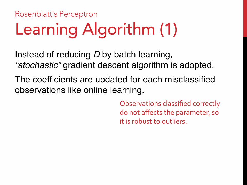
Learning Algorithm (1) Instead of reducing D by batch learning, “stochastic” gradient descent algorithm is adopted. "The coefficients are updated for each misclassified observations like online learning."

Rosenblatt's Perceptron
Learning Algorithm (1) Instead of reducing D by batch learning, “stochastic” gradient descent algorithm is adopted. "The coefficients are updated for each misclassified observations like online learning."
Rosenblatt's Perceptron
Learning Algorithm (1) Instead of reducing D by batch learning, “stochastic” gradient descent algorithm is adopted. "The coefficients are updated for each misclassified observations like online learning."
Observations classified correctly do not affects the parameter, so it is robust to outliers.

Rosenblatt's Perceptron
Learning Algorithm (1) Instead of reducing D by batch learning, “stochastic” gradient descent algorithm is adopted. "The coefficients are updated for each misclassified observations like online learning.""Thus, coefficients will be updated based not on D but on single"D(β,β0) = !y(" β + β0)
Rosenblatt's Perceptron
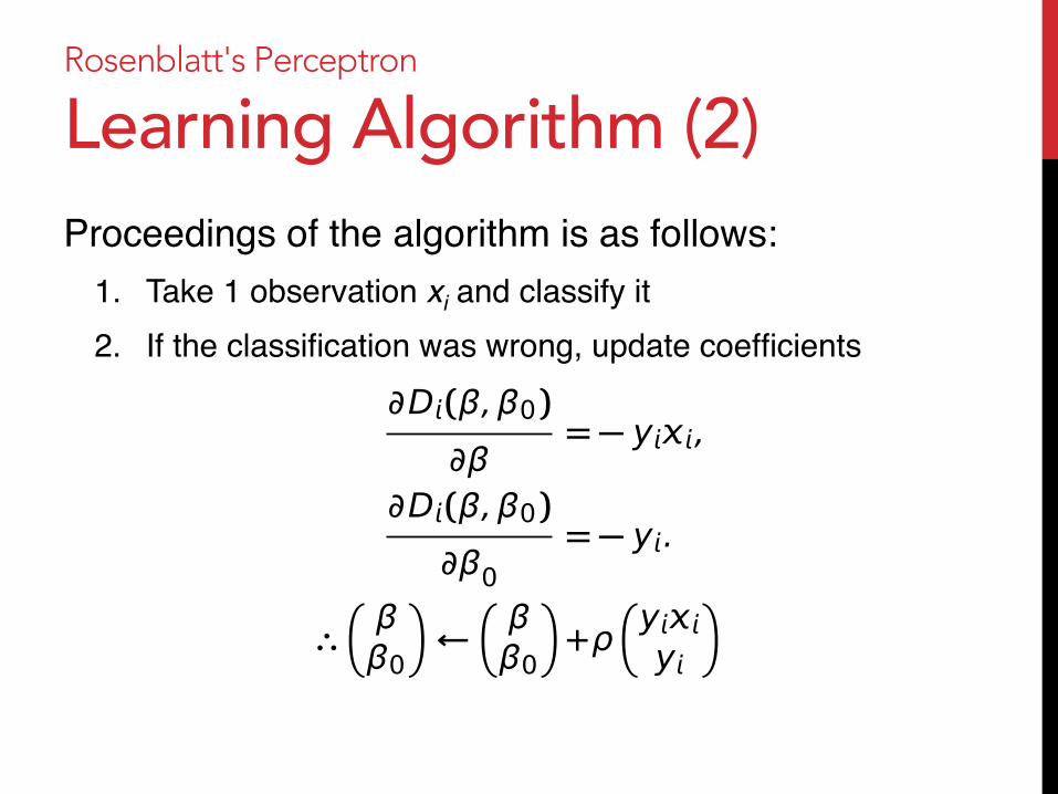
Learning Algorithm (2) Proceedings of the algorithm is as follows:"
Rosenblatt's Perceptron
Learning Algorithm (2) Proceedings of the algorithm is as follows:"
1. Take 1 observation xi and classify it"
Rosenblatt's Perceptron
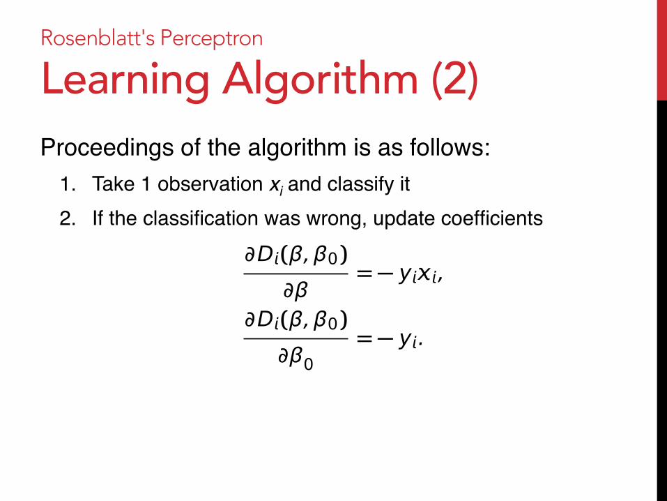
Learning Algorithm (2) Proceedings of the algorithm is as follows:"
1. Take 1 observation xi and classify it"2. If the classification was wrong, update coefficients"
∂D(β,β0)
∂β= ! y,
∂D(β,β0)
∂β0= ! y.
!!ββ0
""!ββ0
"+ρ!yy
"00
Rosenblatt's Perceptron
Learning Algorithm (2) Proceedings of the algorithm is as follows:"
1. Take 1 observation xi and classify it"2. If the classification was wrong, update coefficients"
∂D(β,β0)
∂β= ! y,
∂D(β,β0)
∂β0= ! y.
!!ββ0
""!ββ0
"+ρ!yy
"
Rosenblatt's Perceptron
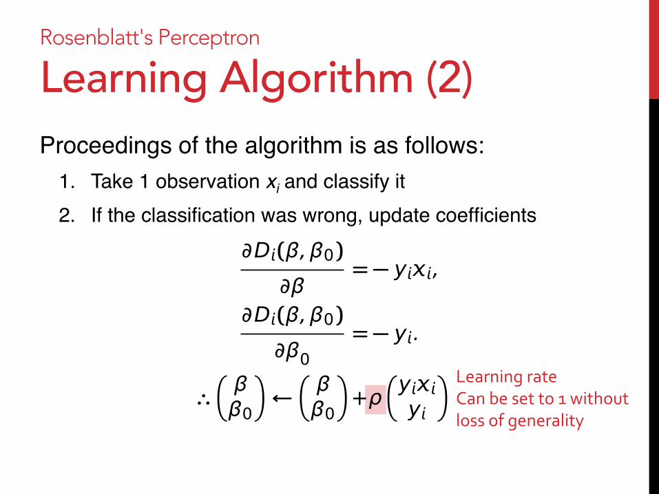
Learning Algorithm (2) Proceedings of the algorithm is as follows:"
1. Take 1 observation xi and classify it"2. If the classification was wrong, update coefficients"
∂D(β,β0)
∂β= ! y,
∂D(β,β0)
∂β0= ! y.
!!ββ0
""!ββ0
"+ρ!yy
" Learning rate Can be set to 1 without loss of generality
Rosenblatt's Perceptron
Learning Algorithm (3) Updating parameter may lead misclassifications of other correctly-classified observations."Therefore, although each update reduces each Di , it can increase total D."

Rosenblatt's Perceptron
Learning Algorithm (3) Updating parameter may lead misclassifications of other correctly-classified observations."Therefore, although each update reduces each Di , it can increase total D."
Rosenblatt's Perceptron
Convergence Theorem If data is linear separable learning of perceptron terminates in finite steps. "Otherwise, learning never terminates.""
Rosenblatt's Perceptron
Convergence Theorem If data is linear separable learning of perceptron terminates in finite steps. "Otherwise, learning never terminates."

Rosenblatt's Perceptron
Convergence Theorem If data is linear separable learning of perceptron terminates in finite steps. "Otherwise, learning never terminates.""
However, in practical, it is difficult to know if"• the data is not linear separable and never converge"• or the data is linear separable but time-consuming"
"
"
Rosenblatt's Perceptron
Convergence Theorem If data is linear separable learning of perceptron terminates in finite steps. "Otherwise, learning never terminates.""
However, in practical, it is difficult to know if"• the data is not linear separable and never converge"• or the data is linear separable but time-consuming"
"
In addition, the solution is not unique depending on the initial value or data order.""

Today's topics þ Logistic regression (contd.)"
þ On the analogy with Least Squares Fitting"þ Logistic regression vs. LDA"
¨ Separating Hyperplane"¨ Rosenblatt's Perceptron"¨ Optimal Hyperplane"
Today's topics þ Logistic regression (contd.)"
þ On the analogy with Least Squares Fitting"þ Logistic regression vs. LDA"
¨ Separating Hyperplane"þ Rosenblatt's Perceptron"¨ Optimal Hyperplane"
Optimal Hyperplane
Derivation of KKT cond. (1) This section could be hard for some audience.""To make story bit clearer, let us study general on optimization problem. The theme is:"
Optimal Hyperplane
Derivation of KKT cond. (1) This section could be hard for some audience.""To make story bit clearer, let us study general on optimization problem. The theme is:"
Duality and KKT condition for optimization problem"
Optimal Hyperplane
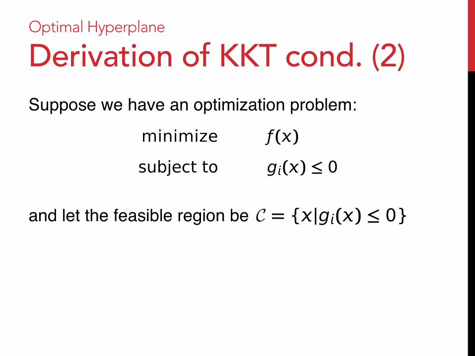
Derivation of KKT cond. (2) Suppose we have an optimization problem:""""and let the feasible region be"
minimize ƒ ()
subject to g() ! 0
C = {|g() ! 0}

Optimal Hyperplane
Derivation of KKT cond. (3) On the region of optimization, relaxation is the technique often used to make problem easier.""

Optimal Hyperplane
Derivation of KKT cond. (3) On the region of optimization, relaxation is the technique often used to make problem easier.""Lagrange relaxation, as done below, is one of that:"" minimize L(, y) = ƒ () +
!
yg()
subject to y ! 0.

Optimal Hyperplane
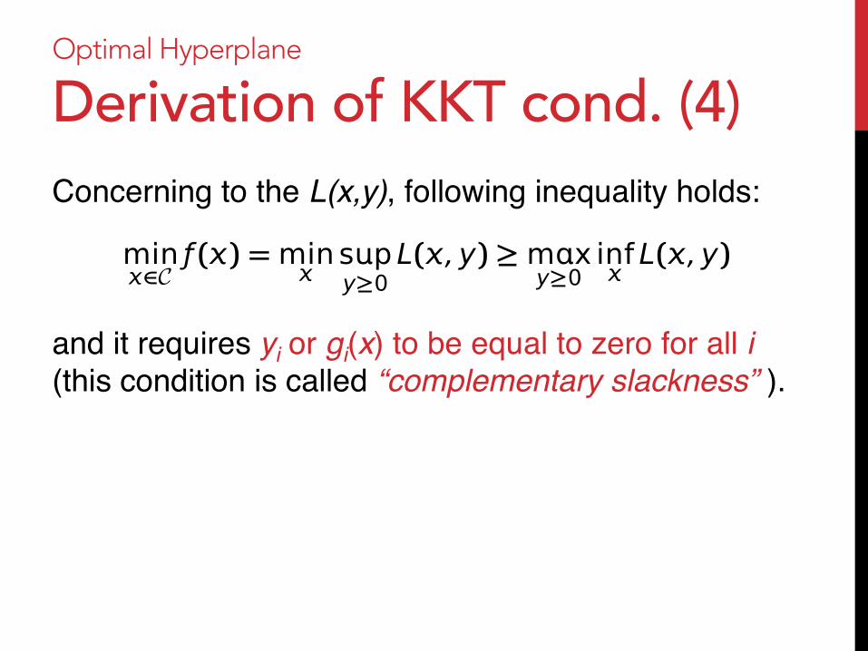
Derivation of KKT cond. (4) Concerning to the L(x,y), following inequality holds:"""and it requires yi or gi(x) to be equal to zero for all i (this condition is called “complementary slackness” )."
min!C
ƒ () =min
spy"0
L(, y) "mxy"0
infL(, y)
Optimal Hyperplane
Derivation of KKT cond. (4) Concerning to the L(x,y), following inequality holds:"""and it requires yi or gi(x) to be equal to zero for all i (this condition is called “complementary slackness” )."
min!C
ƒ () =min
spy"0
L(, y) "mxy"0
infL(, y)

Optimal Hyperplane
Derivation of KKT cond. (4) Concerning to the L(x,y), following inequality holds:"""and it requires yi or gi(x) to be equal to zero for all i (this condition is called “complementary slackness” ).""According to the inequality, maximizing infx L(x,y) tells us the lower boundary for the original problem."
min!C
ƒ () =min
spy"0
L(, y) "mxy"0
infL(, y)
Optimal Hyperplane
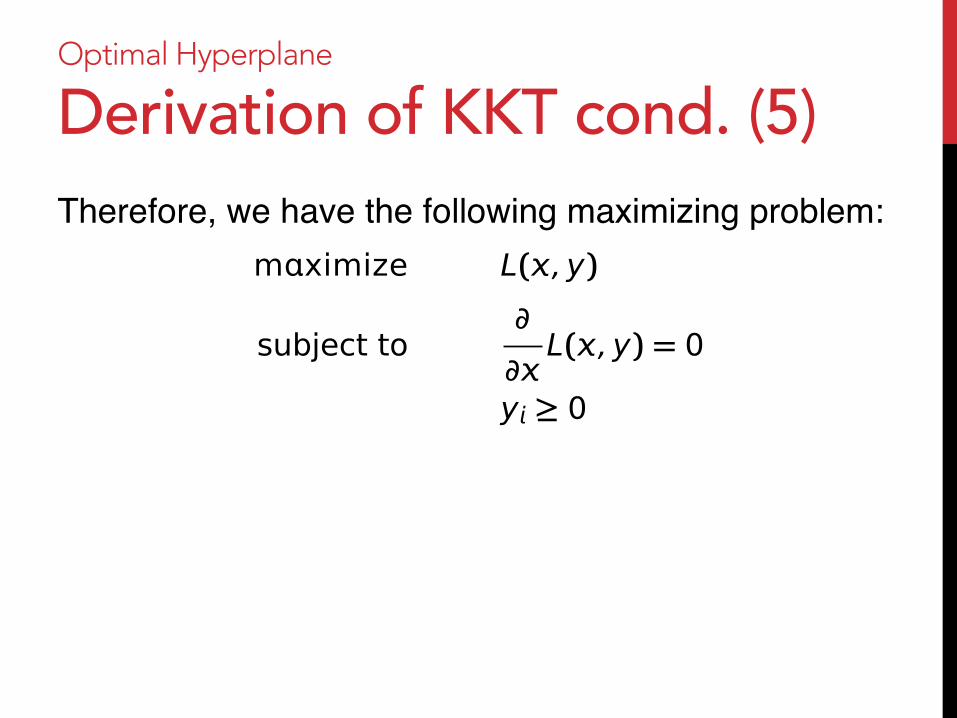
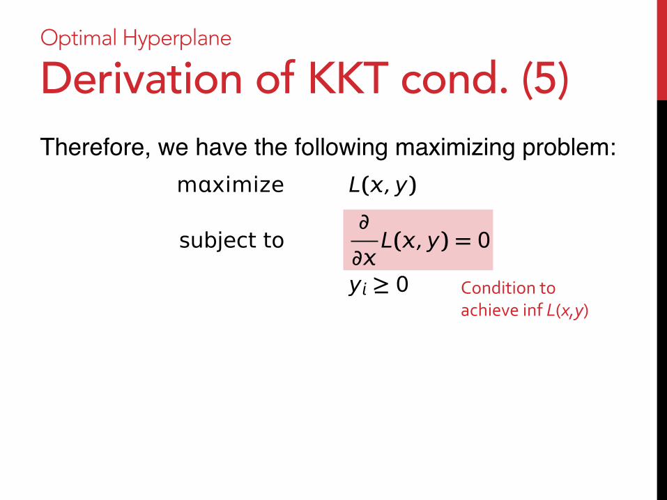
Derivation of KKT cond. (5) Therefore, we have the following maximizing problem:"""""
mximize L(, y)
subject to∂
∂L(, y) = 0
y ! 0
Optimal Hyperplane
Derivation of KKT cond. (5) Therefore, we have the following maximizing problem:"""""
mximize L(, y)
subject to∂
∂L(, y) = 0
y ! 0 Condition to achieve inf L(x,y)
Optimal Hyperplane
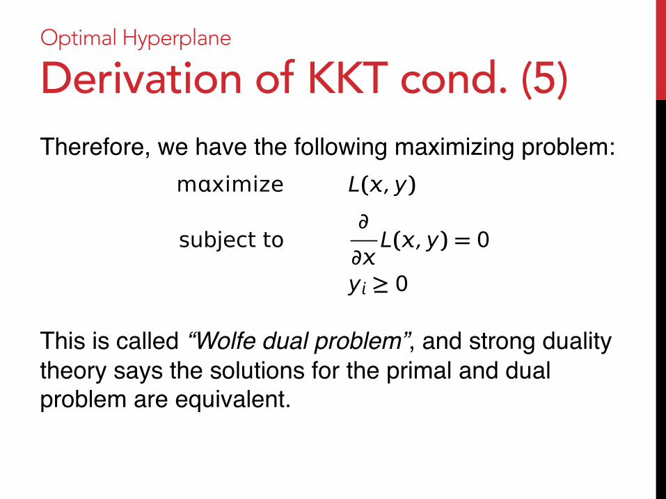
Derivation of KKT cond. (5) Therefore, we have the following maximizing problem:"""""This is called “Wolfe dual problem”, and strong duality theory says the solutions for the primal and dual problem are equivalent."
mximize L(, y)
subject to∂
∂L(, y) = 0
y ! 0

Optimal Hyperplane
Derivation of KKT cond. (5) Therefore, we have the following maximizing problem:"""""This is called “Wolfe dual problem”, and strong duality theory says the solutions for the primal and dual problem are equivalent."
mximize L(, y)
subject to∂
∂L(, y) = 0
y ! 0

Optimal Hyperplane
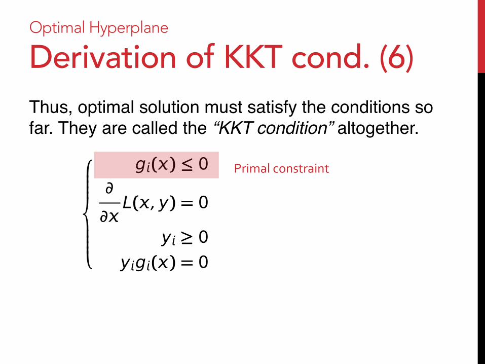
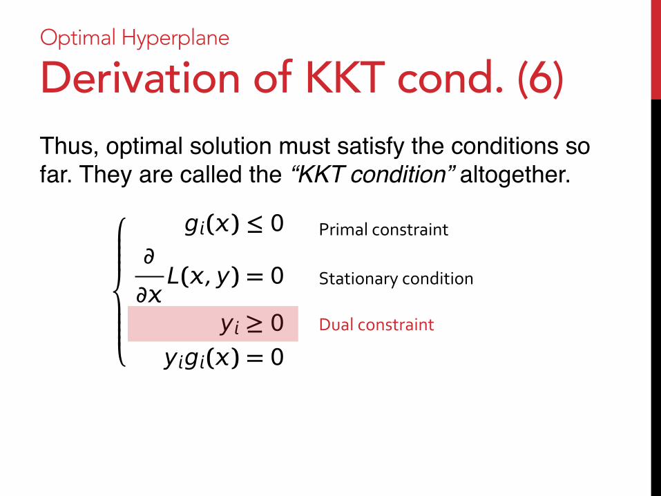
Derivation of KKT cond. (6) Thus, optimal solution must satisfy the conditions so far. They are called the “KKT condition” altogether."!""""#""""$
g() ! 0∂
∂L(, y) = 0
y " 0yg() = 0
Optimal Hyperplane
Derivation of KKT cond. (6) Thus, optimal solution must satisfy the conditions so far. They are called the “KKT condition” altogether."!""""#""""$
g() ! 0∂
∂L(, y) = 0
y " 0yg() = 0
Primal constraint
Optimal Hyperplane
Derivation of KKT cond. (6) Thus, optimal solution must satisfy the conditions so far. They are called the “KKT condition” altogether."!""""#""""$
g() ! 0∂
∂L(, y) = 0
y " 0yg() = 0
Primal constraint
Stationary condition
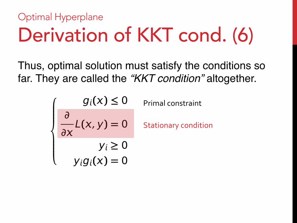
Optimal Hyperplane
Derivation of KKT cond. (6) Thus, optimal solution must satisfy the conditions so far. They are called the “KKT condition” altogether."!""""#""""$
g() ! 0∂
∂L(, y) = 0
y " 0yg() = 0
Primal constraint
Stationary condition
Dual constraint
Optimal Hyperplane
Derivation of KKT cond. (6) Thus, optimal solution must satisfy the conditions so far. They are called the “KKT condition” altogether."!""""#""""$
g() ! 0∂
∂L(, y) = 0
y " 0yg() = 0
Primal constraint
Stationary condition
Dual constraint
Complementary slackness

Optimal Hyperplane
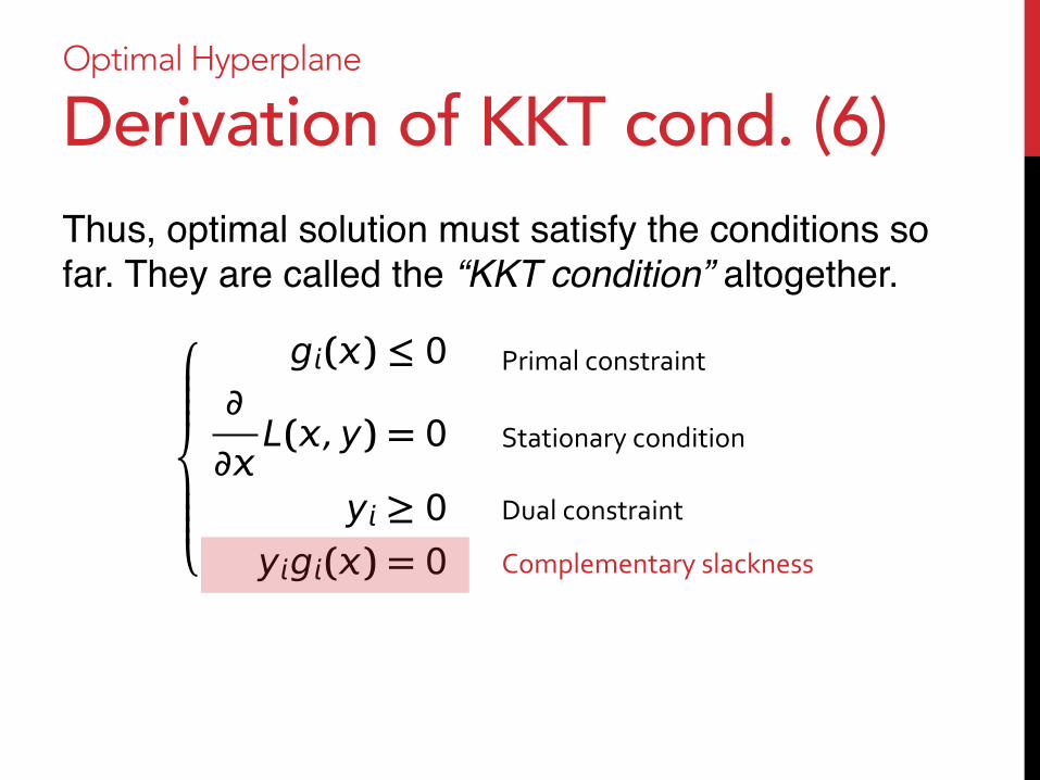
Derivation of KKT cond. (6) Thus, optimal solution must satisfy the conditions so far. They are called the “KKT condition” altogether."!""""#""""$
g() ! 0∂
∂L(, y) = 0
y " 0yg() = 0
Primal constraint
Stationary condition
Dual constraint
Complementary slackness

Optimal Hyperplane
KKT for Opt. Hyperplane (1) We learned about the KKT conditions.""Then, get back to the original problem: finding optimal hyperplane."

Optimal Hyperplane
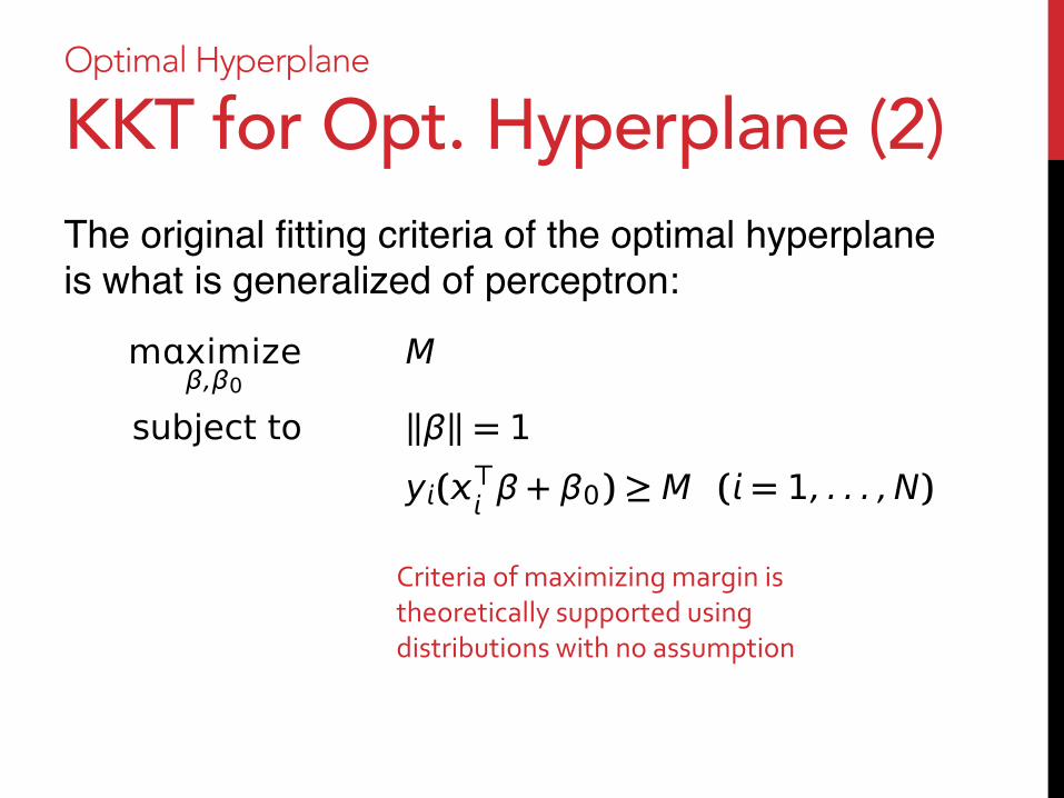
KKT for Opt. Hyperplane (2) The original fitting criteria of the optimal hyperplane is what is generalized of perceptron:"" mximize
β,β0M
subject to !β! = 1
y(" β + β0) # M ( = 1, . . . , N)
Optimal Hyperplane
KKT for Opt. Hyperplane (2) The original fitting criteria of the optimal hyperplane is what is generalized of perceptron:"" mximize
β,β0M
subject to !β! = 1
y(" β + β0) # M ( = 1, . . . , N)
Criteria of maximizing margin is theoretically supported using distributions with no assumption

Optimal Hyperplane
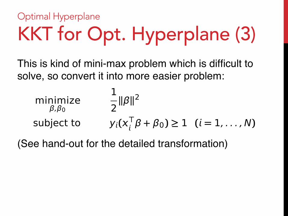
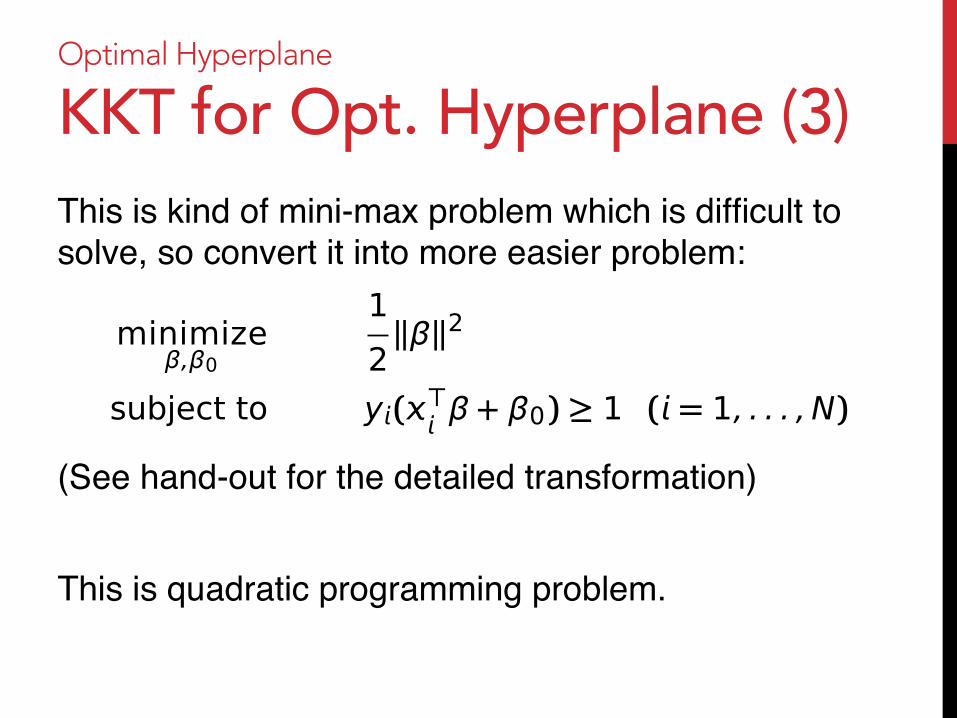
KKT for Opt. Hyperplane (3) This is kind of mini-max problem which is difficult to solve, so convert it into more easier problem:""""
Optimal Hyperplane
KKT for Opt. Hyperplane (3) This is kind of mini-max problem which is difficult to solve, so convert it into more easier problem:""""(See hand-out for the detailed transformation)"
minimizeβ,β0
1
2!β!2
subject to y(" β + β0) # 1 ( = 1, . . . , N)
Optimal Hyperplane
KKT for Opt. Hyperplane (3) This is kind of mini-max problem which is difficult to solve, so convert it into more easier problem:""""(See hand-out for the detailed transformation)""This is quadratic programming problem."
minimizeβ,β0
1
2!β!2
subject to y(" β + β0) # 1 ( = 1, . . . , N)

Optimal Hyperplane
KKT for Opt. Hyperplane (4) To make use of KKT condition, let's make object function into Lagrange function:"
Lp =1
2!β!2 "
N!
=1α"y(# β + β0) " 1
#

Optimal Hyperplane
KKT for Opt. Hyperplane (5) Thus, the KKT condition is:"!""""""""""""#""""""""""""$
y(! β + β0) " 1 ( = 1, . . . , N),
β =N%
=1αy,
0 =N%
=1αy,
α " 0 ( = 1, . . . , N),
α&y(! β + β0) # 1
'= 0 ( = 1, . . . , N),

Optimal Hyperplane
KKT for Opt. Hyperplane (5) Thus, the KKT condition is:"""
"
""
""
"Solution is obtained by solving this."
!""""""""""""#""""""""""""$
y(! β + β0) " 1 ( = 1, . . . , N),
β =N%
=1αy,
0 =N%
=1αy,
α " 0 ( = 1, . . . , N),
α&y(! β + β0) # 1
'= 0 ( = 1, . . . , N),

Optimal Hyperplane
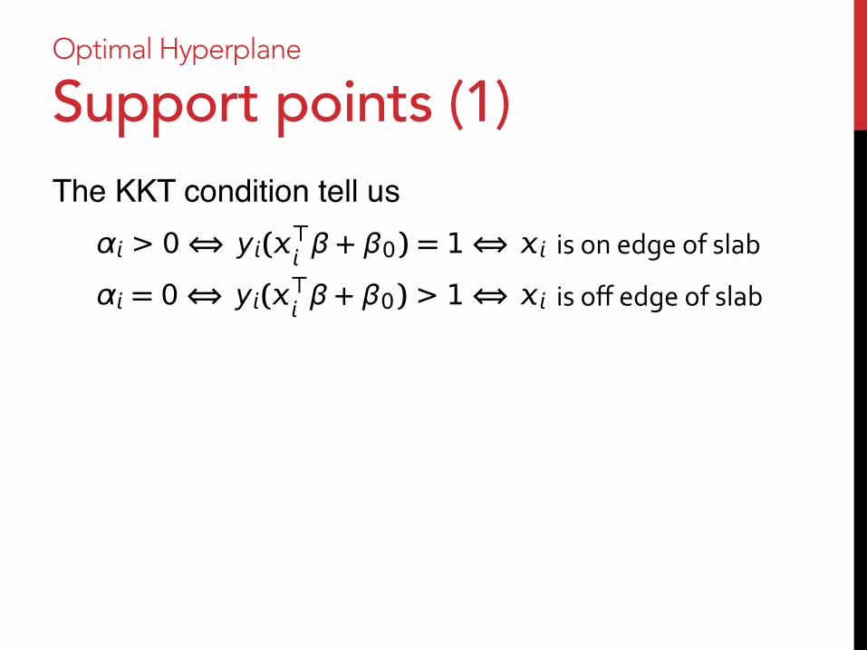
Support points (1) The KKT condition tell us""""
α > 0! y(" β + β0) = 1!
α = 0! y(" β + β0) > 1!
is on edge of slab
is off edge of slab

Optimal Hyperplane
Support points (1) The KKT condition tell us""""
α > 0! y(" β + β0) = 1!
α = 0! y(" β + β0) > 1!
is on edge of slab
is off edge of slab

Optimal Hyperplane
Support points (1) The KKT condition tell us""""
α > 0! y(" β + β0) = 1!
α = 0! y(" β + β0) > 1!
is on edge of slab
is off edge of slab
Optimal Hyperplane
Support points (1) The KKT condition tell us""""
α > 0! y(" β + β0) = 1!
α = 0! y(" β + β0) > 1!
is on edge of slab
is off edge of slab

Optimal Hyperplane
Support points (1) The KKT condition tell us""""Those points on the edge of the slab is called “support points” (or “support vectors” )."
α > 0! y(" β + β0) = 1!
α = 0! y(" β + β0) > 1!
is on edge of slab
is off edge of slab
Optimal Hyperplane
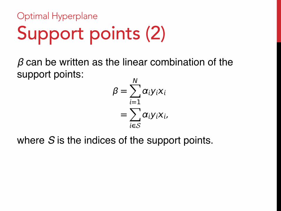
Support points (2) β can be written as the linear combination of the support points:""""where S is the indices of the support points."
β =N!
=1αy
=!
!Sαy,
Optimal Hyperplane
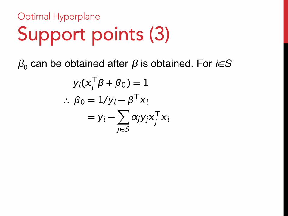
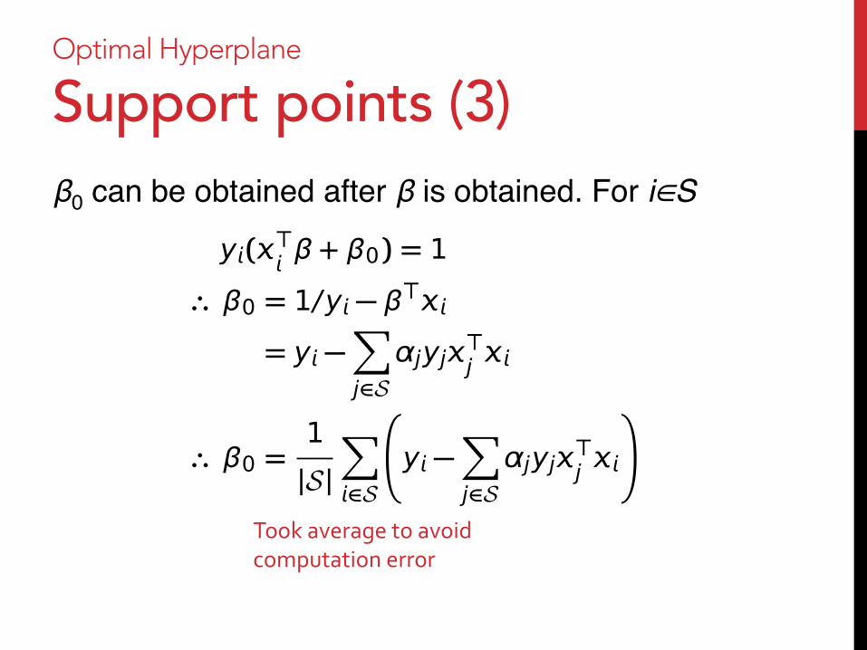
Support points (3) β0 can be obtained after β is obtained. For i∈S"
y(! β + β0) = 1
! β0 = 1/y " β!= y "
!
j#Sαjyj!j
! β0 =1
|S |!
#S
"y "
!
j#Sαjyj!j
#
00
Optimal Hyperplane
Support points (3) β0 can be obtained after β is obtained. For i∈S"
y(! β + β0) = 1
! β0 = 1/y " β!= y "
!
j#Sαjyj!j
! β0 =1
|S |!
#S
"y "
!
j#Sαjyj!j
#
Took average to avoid computation error
Optimal Hyperplane
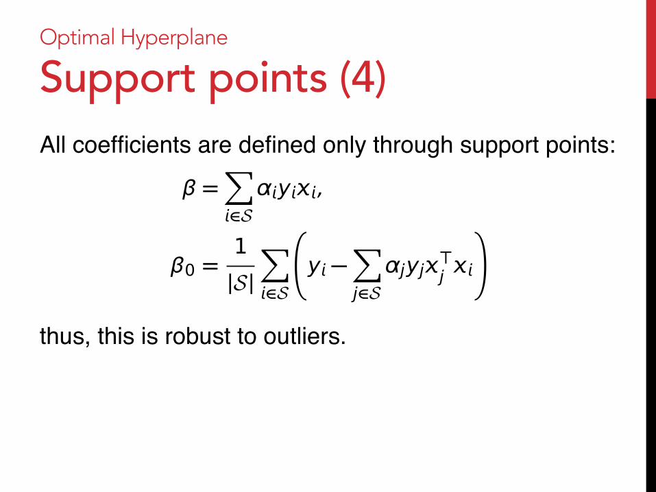
Support points (4) All coefficients are defined only through support points:"""""thus, this is robust to outliers.""
β =!
!Sαy,
β0 =1
|S |!
!S
"y "
!
j!Sαjyj#j
#

Optimal Hyperplane
Support points (4) All coefficients are defined only through support points:"""""thus, this is robust to outliers.""
However, do not forget that which will be support points is defined using all data points."
β =!
!Sαy,
β0 =1
|S |!
!S
"y "
!
j!Sαjyj#j
#

Today's topics þ Logistic regression (contd.)"
þ On the analogy with Least Squares Fitting"þ Logistic regression vs. LDA"
¨ Separating Hyperplane"þ Rosenblatt's Perceptron"¨ Optimal Hyperplane"
Today's topics þ Logistic regression (contd.)"
þ On the analogy with Least Squares Fitting"þ Logistic regression vs. LDA"
¨ Separating Hyperplane"þ Rosenblatt's Perceptron"þ Optimal Hyperplane"
Today's topics þ Logistic regression (contd.)"
þ On the analogy with Least Squares Fitting"þ Logistic regression vs. LDA"
þ Separating Hyperplane"þ Rosenblatt's Perceptron"þ Optimal Hyperplane"

Summary LDA Logistic
Regression Perceptron Optimal Hyperplane
With linear separable data Training error may occur
True separator found, but coef. may be infinite
True separator found, but not unique
Best separator found
With non-linear separable data Work well Work well Algorithm never
stop Not feasible
With outliers Not robust Robust Robust Robust