1

Loan Portfolio Performance and El Niño, an Intervention Analysis

Benjamin Collier, Ani L. Katchova, and Jerry R. Skees1

This is an electronic version of a journal article, please cite as: Collier, B., A.L. Katchova, and J. Skees. “Loan Portfolio Performance and El Nino, an

Intervention Analysis.” Agricultural Finance Review 71(2011):98-119.

Selected Paper prepared for presentation at the Southern Agricultural Economics Association

Annual Meeting, Orlando, FL, February 6-9, 2010

Copyright 2010 by [Collier, Katchova, and Skees]. All rights reserved. Readers may make verbatim copies of this document for non-commercial purposes by any means, provided this

copyright notice appears on all such copies.

1 Benjamin Collier is a doctoral applicant, Ani Katchova is an assistant professor, and Jerry Skees is the H.B. Price Professor of Policy and Risk in the Department of Agricultural Economics at the University of Kentucky.

2

Loan Portfolio Performance and El Niño, an Intervention Analysis

Abstract Purpose – This paper illustrates that natural disasters can significantly threaten financial institutions serving the poor. The authors test the case of a microfinance institution (MFI) in Northern Peru, where severe El Niño events create catastrophic flooding. Design/methodology/approach – Portfolio-level, monthly data from January 1994 to October 2008 were examined using an intervention analysis. The paper tested whether the 1997-1998 El Niño increased problem loans and estimated the magnitude of the effect. Findings – The results indicate El Niño significantly increased problem loans, specifically the level of restructured loans. While restructured loans averaged 0.5 percent of the total loan portfolio before the El Niño, the estimated cumulative effect of El Niño indicates that an additional 3.6 percent of the portfolio value was restructured due to this event. Research limitations/implications – Future research could build on these results by modeling insurance-type mechanisms for the MFI. Additional research that replicates these analyses in another context would be highly valuable for comparison across natural disasters and financial institutions. Practical implications – The findings demonstrate that the correlated risk exposure of many small borrowers can significantly affect the lender and the importance of considering bank management in assessing disaster risk of a financial institution. Social implications – Lender strategies to minimize losses may require long-term restructuring that perpetuates the effects of the disaster in the community. Originality/value – This paper may be of particular value to researchers and practitioners hoping to improve the effectiveness and efficiency of MFIs concentrated in regions exposed to natural disaster risk. Keywords: Financial institutions, Natural disasters, Portfolio investment, Peru

3

Loan Portfolio Performance and El Niño, an Intervention Analysis

Natural disasters can significantly threaten financial institutions serving the poor. Moreover,

without proper assessment of natural disaster risk, microfinance institutions (MFIs) experience

the risk of either underestimating their exposure (threatening long-term stability) or

overestimating their exposure (unnecessarily limiting access to credit). Thus, methodologies to

enhance assessment of natural disaster risk for MFIs are needed. This study estimates the effects

of a natural disaster on the lending portfolio performance of a financial institution serving the

poor. Specifically, we have identified an MFI in Piura, a region in northern Peru severely

affected by El Niño. Extreme El Niño events like those in 1982-83 and 1997-98 create

catastrophic flooding that destroys transportation infrastructure, productive assets, crops, and

private homes and disrupts the livelihoods of households engaged in a wide range of activities.

Background: Banking and Natural Disaster Risk

Access to financial services, especially credit, has played an increasingly important role in

development economics theory and applications in the past four decades. Many households have

gained access to microcredit and increasingly sophisticated approaches are being adopted to

enhance the performance of financial institutions serving the poor. For example in some regions,

banking regulators are governing financial institutions providing microfinance

(http://www.sbs.gob.pe/portalSBS/), and credit rating agencies (e.g., Planet Rating and

MicroRate) have emerged that specialize in MFIs. Such advancements are generally intended to

enhance the efficiency, effectiveness, and stability of microfinance providers with the end result

of increasing access to financial services at better terms (e.g., lower interest rates for loans). Yet,

in this context, many challenges remain to providing microcredit to the poor. One such challenge

is natural disaster risk.

4

Natural disasters result in spatially correlated losses that can substantially affect the

lending portfolio, especially if the portfolio is geographically concentrated (Bessis, 1998; Skees

and Barnett, 2006). In this context, correlated risks cannot be completely managed by increasing

the number of borrowers if all borrowers have some exposure. Figure 1 presents a stylized

version of this problem. In this example, the bank lends to n identical borrowers that are exposed

to both idiosyncratic risk (e.g., death of the breadwinner, health problems in the household, etc.)

and correlated risk (e.g., severe weather risk, price risk, etc.). As n increases, the concentration of

the portfolio declines and the bank is less exposed to the idiosyncratic risks of borrowers;

however, as the figure shows, the correlated risk exposure of the bank remains (see also

Katchova and Barry, 2005, Garside et al., 1999).

Natural disasters are categorized as a component of operational risk by banking

regulators. There has been increasing recognition that 1) assessing and measuring operational

risk is an important aspect of protecting bank solvency; and 2) the risks facing financial

institutions (credit risk, market risk, operational risk, etc.) are interrelated (Basel Committee on

Banking Supervision, 2004; Greuning and Bratanovic, 2009). To manage correlated risks,

banking regulators require that lenders maintain certain levels of capital. Still, lenders may be

uncertain of their level of exposure to a natural disaster, as assessing this risk can be quite

difficult (Charnobai and Rachev, 2006; Garside et al., 1999). Holding too little capital threatens

the solvency of the lender when a catastrophe occurs. However, because banks typically operate

on small profit margins but are highly leveraged (low capital-to-asset ratios), holding larger-

than-necessary capital reserves can represent significant opportunity costs for lenders (Greuning

and Bratanovic, 2009).

Intervention Analysis

5

A common methodology used to examine the effects of catastrophic events on business

operations is intervention analysis. These analyses use time-series data and identify the

occurrence of the event with dummy variables. The immediate and long-term effects of the event

can then be modeled using the specification of the time-series model. Intervention analysis has

been used to estimate the effects of a variety of disasters including the effects of the September

11 terrorist attacks on the airline industry (Guzhva, 2008); the 1986 nuclear disaster in

Chernobyl on tourism in Sweden (Hultkrantz and Olsson, 1997); Hurricane Hugo on the business

of a public hospital (Fox, 1996) and lumber prices (Prestemon and Holmes, 2000) in South

Carolina; and floods, cyclones, earthquakes, and other disasters on daily values for an Australian

capital market index (Worthington and Valadkhani, 2004).

In the context of financial institutions, intervention analysis has primarily been used to

assess the effects of policy and regulation changes or how well capital markets integrate

information. For example, Ortiz (1983) examines the effects of the devaluation of the Mexican

peso on the ratio of U.S. dollars to pesos held as savings deposits in Mexican banks; Allen and

Wilhelm (1988) analyze the effects of the 1980 Depository Institutions Deregulatory and

Monetary Control Act on the market values of deposit-taking institutions; and Philippatos and

Viswanathan (1991) examine the effects of the 1987 Brazilian debt moratorium announcement

on the market value of U.S. banks. Much of the research on financial institutions has

concentrated on the effects of an event on stock prices for publicly traded firms.

A wealth of literature exists regarding the effect of a specific event on the value of a

financial institution in the event studies literature (MacKinlay, 1997). In some contexts,

intervention analysis and event study methodologies are quite similar; however, generally

intervention analysis examines a specific event while event studies often attempt to estimate the

6

effects of a type of event. As a result, event studies more typically examine several event

occurrences and rely on a contemporaneous baseline (e.g., the S&P 500 if the study is examining

movements in stock prices) as a control parameter (Binder, 1998). El Niño, the event of interest

in this study, has such significant effects on the banking industry throughout Peru limiting the

ability to find a suitable contemporaneous control group. Additionally, this study examines the

effect of a single extreme El Niño on one financial institution. Therefore, an intervention

analyses methodology was chosen.

In sum, while intervention analysis and similar methodologies have been used to estimate

the effects of catastrophic events on business performance, and these methodologies have been

used to estimate the effects of a variety of events on bank performance, we are unaware of any

published study estimating the effects of a catastrophic event on lender portfolio performance,

especially for a financial institution serving the poor.

The purpose of this paper is to assess exposure of an MFI in Piura to the consequences

associated with the extreme El Niño of 1997-98. Given a long time series, the effects of El Niño

on the proportions of troubled loans in the lending portfolio (loans that are restructured from

their original terms and loans that are late in payments) can be isolated and inferences can be

developed regarding the effects of extreme natural disasters like those created by El Niño. The

paper has two objectives. The first objective is to test a hypothesis that the 1997-98 El Niño

significantly increased the levels of late and/or restructured loans in the lending portfolio. A

significant increase would consist of a pattern of (one-tailed) statistically significant increases in

late and/or restructured loans in the months leading up to, during, and after the 1997-98 El Niño.

The pattern of results for late and restructured loans will be analyzed for additional insights into

when El Niño began affecting the lending portfolio and what combination of late and

7

restructured loans the MFI used to address these problems. The second objective is to estimate

the magnitude of the effect on troubled loans. We anticipate that these analyses will highlight the

significant operational risk associated with such a natural disaster to geographically concentrated

financial institutions.

Piura

Piura is a diverse geographic region in northwestern Peru with a population of 1.7 million

(Instituto Nacional de Estadística e Informática, 2007). Agriculture is an important livelihood in

the region, employing 37 percent of the workforce, which almost exclusively works on small

farms of less than 10 hectares (Instituto Nacional de Estadística e Informática, 2007; Oft, 2009;

Trivelli, 2006). Along the Pacific coast, Piura is an arid region with good soils and irrigated

agriculture, making it one of the most productive agricultural regions in Peru. Moving from the

coast eastward, the region is dominated by trees crops such as coffee and cocoa as the terrain

changes quickly to semi-tropical small mountains. Beyond these regions are the high Andes

where agriculture supports local consumption. Fifty-four percent of the population in Piura is at

or below the poverty line (Instituto Nacional de Estadística e Informática, 2007). Credit is an

important component of livelihood enhancement for households in Piura, and organizations

providing small-enterprise loans have grown significantly in recent years. For example, the loan

portfolio of Caja Piura, one of the largest municipal banks in Piura and the lender whose

portfolio is analyzed in this study, grew from USD 2.6 million in January 1994 to USD 312

million in October 2008 (http://www.sbs.gob.pe/portalSBS/). Caja Piura lends to a variety of

commercial and retail clients with an emphasis in small-enterprise loans; its average loan size is

USD 3,182 (Trivelli, 2006).

Piura is severely affected by El Niño (United States Agency for International

8

Development, 2006). El Niño events occur when ocean currents and trade winds deviate from

their normal cycle in the Southern Pacific, resulting in elevated sea surface temperatures and

warmer trade winds off the coast of Peru (McPhaden, 2003; Oldenborgh et al., 2005). These

warm trade winds meet cool air descending from the Andes Mountains causing excess rainfall

from December through April in Piura. Signs of an impending El Niño occur several months

before extreme rainfall begins (McPhaden, 2003). During extreme El Niño events such as those

in 1982-83 and 1997-98, catastrophic flooding occurred, beginning early in the year, about

February 1983 and February 1998. In these years, rainfall was 40 times above normal for

January to April, and volume in the Piura River was 41 times above its median volume. Experts

predict such an extreme El Niño may now occur as frequently as 1 in every 15 years (Skees and

Murphy, 2009).

Orlove et al. (2004) report rumors of an impending El Niño event as early as March of

1997, and the Peruvian government announced the potential for an El Niño event in June 1997.

Signals become stronger as the period of excess rainfall approaches, and forecasting transitions

from whether or not an El Nino event will occur to predicting the magnitude of the event. Ex

post surveys conducted by Orlove et al. (2004) indicated that many households in Peru were

unable to identify the specific month when they first heard the forecast of an impending El Niño,

but roughly 60 percent of the survey reported having heard by June 1997. Orlove et al., (2004)

also found many households engaged in risk mitigating activities such as securing their homes

before extreme rainfall and flooding began. They note that, especially for those in vulnerable

economic sectors such as fishing, households were making these investments when entering a

time of expected reduced income due to the impending natural disaster. These conditions put

additional pressure on household budgets and would increase the opportunity cost of repaying

9

loans. Thus, it may be the case that competition for household funds reduced repayment rates

even in the months leading up to the catastrophic flooding.

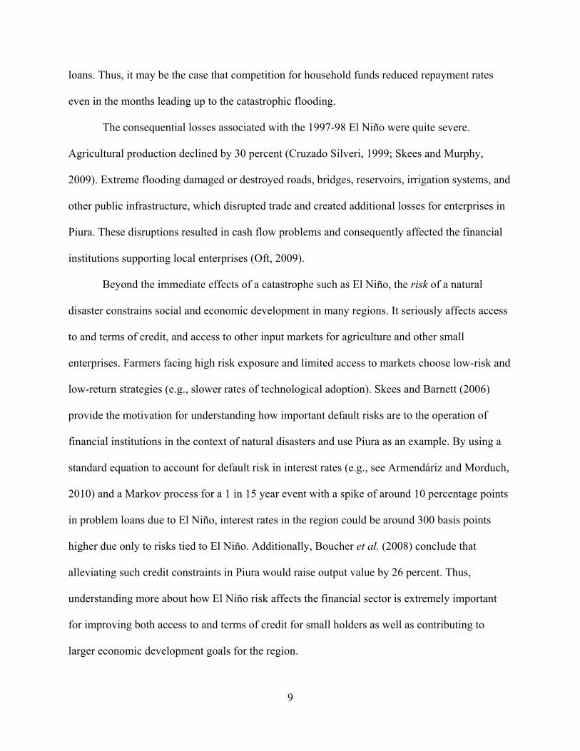
The consequential losses associated with the 1997-98 El Niño were quite severe.

Agricultural production declined by 30 percent (Cruzado Silveri, 1999; Skees and Murphy,

2009). Extreme flooding damaged or destroyed roads, bridges, reservoirs, irrigation systems, and

other public infrastructure, which disrupted trade and created additional losses for enterprises in

Piura. These disruptions resulted in cash flow problems and consequently affected the financial

institutions supporting local enterprises (Oft, 2009).

Beyond the immediate effects of a catastrophe such as El Niño, the risk of a natural

disaster constrains social and economic development in many regions. It seriously affects access

to and terms of credit, and access to other input markets for agriculture and other small

enterprises. Farmers facing high risk exposure and limited access to markets choose low-risk and

low-return strategies (e.g., slower rates of technological adoption). Skees and Barnett (2006)

provide the motivation for understanding how important default risks are to the operation of

financial institutions in the context of natural disasters and use Piura as an example. By using a

standard equation to account for default risk in interest rates (e.g., see Armendáriz and Morduch,

2010) and a Markov process for a 1 in 15 year event with a spike of around 10 percentage points

in problem loans due to El Niño, interest rates in the region could be around 300 basis points

higher due only to risks tied to El Niño. Additionally, Boucher et al. (2008) conclude that

alleviating such credit constraints in Piura would raise output value by 26 percent. Thus,

understanding more about how El Niño risk affects the financial sector is extremely important

for improving both access to and terms of credit for small holders as well as contributing to

larger economic development goals for the region.

10

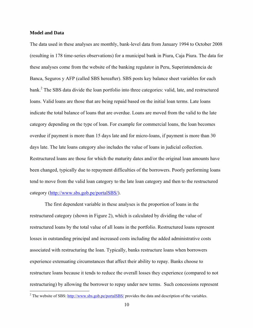
Model and Data

The data used in these analyses are monthly, bank-level data from January 1994 to October 2008

(resulting in 178 time-series observations) for a municipal bank in Piura, Caja Piura. The data for

these analyses come from the website of the banking regulator in Peru, Superintendencia de

Banca, Seguros y AFP (called SBS hereafter). SBS posts key balance sheet variables for each

bank.2 The SBS data divide the loan portfolio into three categories: valid, late, and restructured

loans. Valid loans are those that are being repaid based on the initial loan terms. Late loans

indicate the total balance of loans that are overdue. Loans are moved from the valid to the late

category depending on the type of loan. For example for commercial loans, the loan becomes

overdue if payment is more than 15 days late and for micro-loans, if payment is more than 30

days late. The late loans category also includes the value of loans in judicial collection.

Restructured loans are those for which the maturity dates and/or the original loan amounts have

been changed, typically due to repayment difficulties of the borrowers. Poorly performing loans

tend to move from the valid loan category to the late loan category and then to the restructured

category (http://www.sbs.gob.pe/portalSBS/).

The first dependent variable in these analyses is the proportion of loans in the

restructured category (shown in Figure 2), which is calculated by dividing the value of

restructured loans by the total value of all loans in the portfolio. Restructured loans represent

losses in outstanding principal and increased costs including the added administrative costs

associated with restructuring the loan. Typically, banks restructure loans when borrowers

experience extenuating circumstances that affect their ability to repay. Banks choose to

restructure loans because it tends to reduce the overall losses they experience (compared to not

restructuring) by allowing the borrower to repay under new terms. Such concessions represent 2 The website of SBS: http://www.sbs.gob.pe/portalSBS/ provides the data and description of the variables.

11

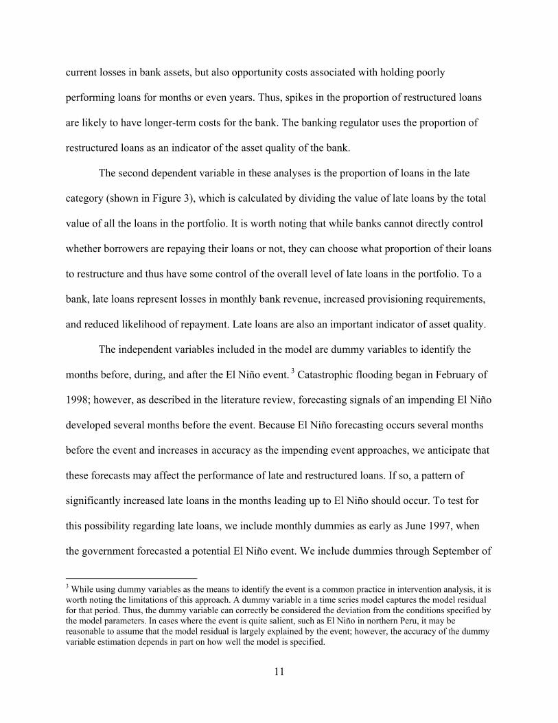
current losses in bank assets, but also opportunity costs associated with holding poorly

performing loans for months or even years. Thus, spikes in the proportion of restructured loans

are likely to have longer-term costs for the bank. The banking regulator uses the proportion of

restructured loans as an indicator of the asset quality of the bank.

The second dependent variable in these analyses is the proportion of loans in the late

category (shown in Figure 3), which is calculated by dividing the value of late loans by the total

value of all the loans in the portfolio. It is worth noting that while banks cannot directly control

whether borrowers are repaying their loans or not, they can choose what proportion of their loans

to restructure and thus have some control of the overall level of late loans in the portfolio. To a

bank, late loans represent losses in monthly bank revenue, increased provisioning requirements,

and reduced likelihood of repayment. Late loans are also an important indicator of asset quality.

The independent variables included in the model are dummy variables to identify the

months before, during, and after the El Niño event. 3 Catastrophic flooding began in February of

1998; however, as described in the literature review, forecasting signals of an impending El Niño

developed several months before the event. Because El Niño forecasting occurs several months

before the event and increases in accuracy as the impending event approaches, we anticipate that

these forecasts may affect the performance of late and restructured loans. If so, a pattern of

significantly increased late loans in the months leading up to El Niño should occur. To test for

this possibility regarding late loans, we include monthly dummies as early as June 1997, when

the government forecasted a potential El Niño event. We include dummies through September of

3 While using dummy variables as the means to identify the event is a common practice in intervention analysis, it is worth noting the limitations of this approach. A dummy variable in a time series model captures the model residual for that period. Thus, the dummy variable can correctly be considered the deviation from the conditions specified by the model parameters. In cases where the event is quite salient, such as El Niño in northern Peru, it may be reasonable to assume that the model residual is largely explained by the event; however, the accuracy of the dummy variable estimation depends in part on how well the model is specified.

12

1998 to account for the possibility that deteriorating loan performance may not occur

immediately after the flooding for loans that mature at the end of a production period.

Because banks experience losses and costs from restructuring loans, we anticipate that if

they use forecasting information in their decision to restructure loans, it will occur later in the

year when forecasting information is stronger. The severity of the El Niño may affect how

significantly they alter the terms of the loan during the restructuring process. We include

monthly dummies from October 1997 through September 1998 for the analyses of restructured

loans,

Examining late and restructured loans concurrently enhances the interpretation of an

effect in either category and provides insights into the management strategies of the bank. For

example, the data may suggest a pattern in which late loans increase during the event then,

several months after the event, the proportion of restructured loans increases. If this pattern

occurred it would likely be an indication that some borrowers had difficulty making loan

payments during El Niño, and that the bank restructured loans for troubled borrowers based on

their reduced repayment capacity due to the event. Alternatively, finding an El Niño effect on the

proportion of late loans but not on restructured loans would likely be an indication that the bank

is taking a passive approach to managing troubled assets in the lending portfolio associated with

El Niño.

Estimation Procedures

The model involves a two step procedure: time series estimation and intervention analysis.

Completing our first objective — testing whether the 1997-98 El Niño significantly increased the

levels of late and/or restructured loans in the lending portfolio — requires fitting a time series

model and testing the monthly dummies for significance. If the effect of El Nino on late and/or

13

restructured loans is significant, completing our second objective — estimating the magnitude of

the effect — requires applying intervention analysis to the results from the time series model.

Fitting the Time-Series Model

We use a Box-Jenkins methodology to fit the time-series model (Box and Jenkins, 1968, see also

Enders, 2004; Greene, 2000; Pindyck and Rubinfeld, 1997). First, we test the stationarity of the

dependent variable (first for proportion of restructured loans then for proportion of late loans).

Stationarity indicates that characteristics of the dependent variable (e.g., mean and variance) are

not changing across the time-series, and therefore can be estimated with fixed coefficients for

each independent variable. If restructured loans or late loans is not stationary, several approaches

can be used to transform the data, the most common of which is taking the first difference of the

dependent variable (Δ = − ). Second, we analyze the data to select the appropriate

time-series model. The intention of the time-series procedures is to create an independent and

identically-distributed process by accounting for autoregressive (AR) and/or moving average

(MA) relationships in the model (see Greene, 2000; Enders, 2004). AR processes are a

relationship between current and previous values of the dependent variable; MA processes are a

relationship between current values of the dependent variable and previous values of the error

term. Thus, the basic time-series model can be written

= + + +

where is the dependent variable, is the intercept term, is the error term, denotes the AR

term, denotes the MA term, is the coefficient for the corresponding AR term, and the is

the coefficient for the corresponding MA term. Time-series models that both correct for

stationarity using differencing and incorporate AR and/or MA terms are referred to as

14

autoregressive integrated moving average (ARIMA) models. We examine the model residuals

using the autocorrelation (ACF) and partial autocorrelation functions (PACF) to estimate the

dependence order (the AR and MA processes) of the model. The ACF and PACF describe

correlations between the dependent variable in the current period and model residuals from

previous periods (see Greene, 2000, or Enders, 2004). Diagnostic tests are also used to identify

the best-fitting model. We use goodness of fit tests including the Akaike Information Criterion

(AIC) and Schwarz Bayesian Information Criterion (SBC), the Ljung-Box Q statistic for white

noise, and the coefficients of the lag variables to assess the models (see Enders, 2004). We then

test the time series model for stability — that is that the autoregressive structure of the model

will not cause it to diverge over time. A necessary condition for stability is ∑ < 1=1 , a

sufficient condition for stability is ∑ < 1=1 (Enders, 2004).

After appropriately fitting the time series model, we use maximum likelihood estimation

to test the coefficients on the monthly dummies to determine if El Niño significantly increases

the proportion of late and/or restructured loans in the lending portfolio. Additionally, the model

can be used to identify the pattern and timing in which troubled loans developed by comparing

the effects on late loans to those on restructured loans. If El Niño has no significant effect, no

additional analyses are needed.

Intervention Analysis

Regarding the second objective, the time series must be altered to improve estimation of the

magnitude of the event. First, we identify and control for extreme values of the dependent

variable that are not associated with the El Niño event of interest — outliers. While controlling

for such outliers should improve the fit of the model, the intervention analysis literature warns of

over-fitting by including too many outliers (e.g., Greene, 2000); therefore, we include up to four

15

outliers with an inclusion criteria that their values must deviate from the mean with significance

level of < 0.01 (two-tailed test). Finally, we re-estimate the time-series model with the outlier

dummies included.4

It should be noted that excluding outliers when testing a null hypothesis truncates the

distribution and biases the results, increasing the likelihood of a significant result. Thus, for our

first objective — a hypothesis test that El Niño significantly increases troubled loans — we

estimate a time series model without outlier dummies. In contrast, when an outlier is clearly not

associated with the event of interest (e.g., in our data if an outlier occurs several years before the

1997-98 El Niño event) including it in the model reduces the precision of the estimate of that

event. Not only do these outliers increase the variance unaccounted for in the model, but they can

affect the estimation of the coefficients and the lag structure of the model. Therefore, for our

second objective — estimating the magnitude of the effect of El Niño on the lending portfolio —

we include outlier dummies to reduce unrelated variance.

The intervention analysis employs the time-series model controlling for outliers by

including dummy variables for the outliers to estimate the effects of the event. We use a

maximum likelihood estimation to assess the effects of the El Niño dummies on the restructured

loans and/or late loans. The magnitudes of the coefficients for the event dummies represent the

immediate effects of the 1997-98 El Niño (Enders, 2004). For example, consider a model with a

one period AR lag = + + + +

Where is an outlier dummy and is an event dummy. The immediate effect of the event is the

4 Consistent with the previous footnote describing the limitations of dummy variables, identifying outliers with dummy variables can have important model implications. An outlier may be an indication of an extreme event unrelated to the event of interest or of an extreme value of an important explanatory variable excluded from the model. When researchers are unable to identify the cause of outlying values, a cautious approach is best as including a large number of outlier dummies may result in over-fitting the model to available observations (see Greene, 2000).

16

coefficient of the dummy variable . We only analyze the effects for the event dummies that

have an immediate effect, that is significant at least at the one-tailed α=0.05 level, in the original

time series model, the model before the outliers are omitted.

We also estimate the long-term effects of the event based on the structure of the time-

series model, specifically, the AR process (Enders, 2004). The AR process indicates how current

values of the dependent variable relate to future values. For example using the one period AR lag

model above, the effect of the dummy variable on the independent variable in the current period

affects the value of the independent variable in the next period because of the AR

structure = + + + +

by substitution for = + ( + + + + ) + + +

Thus, when shocks associated with the event enter the model, their total effects must be

estimated using the AR terms specified in the time-series model. For example, for the model

with one AR lag

= 1 + + +⋯+ =

where is the dependent variable, is the event dummy, is the coefficient on the event

dummy, is the coefficient on the AR variable, and represent future periods in the time-series

( , + 1, + 2,… , + ). Results

In this section, the time-series and intervention analysis procedures described in the previous

section are applied to estimate the effects of the 1997-98 El Niño on the proportion of

17

restructured loans and on the proportion of late loans in the lending portfolio of Caja Piura. The

results are organized around the objectives identified in the introduction — first, we test for a

significant increase in problem loans due to El Niño, then if significant, we estimate the

magnitude of the effect.

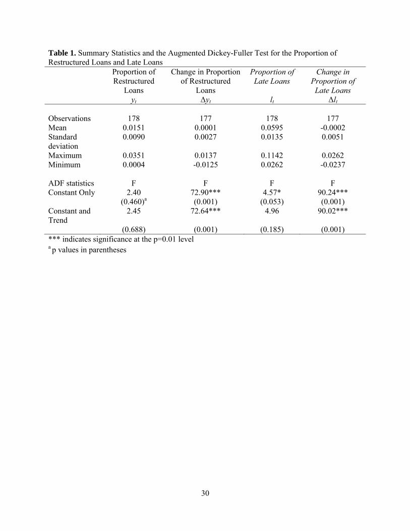
The augmented Dickey-Fuller test was used to assess the stationarity of the proportion of

restructured loans ( ) and the proportion of late loans (lt). This test indicates that the proportion

of restructured loans and the proportion of late loans are both nonstationary; however, the

differenced proportion of restructured loans and the differenced proportion of late loans are

stationary, shown in Table 1. Therefore, we use the differenced proportion of restructured loans,

or change in the proportion of restructured loans (i.e., Δ = − ; shown in Figure 4) and

the change in proportion of late loans (Δlt ) as the dependent variables in the following analyses.

Testing for a Significant Increase in Restructured Loans and/or Late Loans

For restructured loans, inspection of the ACF and PACF and the model fit statistics indicate an

AR lag structure with a lag at the third (Δyt-3) and seventh (Δyt-7 ) periods and no MA terms. The

necessary and sufficient conditions for stability hold for this time-series model. The maximum

likelihood estimation suggests significant effects of the El Niño event on the change in

proportion of restructured loans in December 1997, January, March, April and May 1998,

reported in Table 2. Significant effects in December and January indicate loans were being

restructured before the catastrophic flooding due to El Niño began in February 1998. Significant

effects in March, April, and May 1998 coincide with the major period of flooding due to El

Niño. By June 1998, the proportion of restructured loans seems to have reached a plateau as no

significant increases in the proportion of restructured loans are found in the monthly dummies

after June.

18

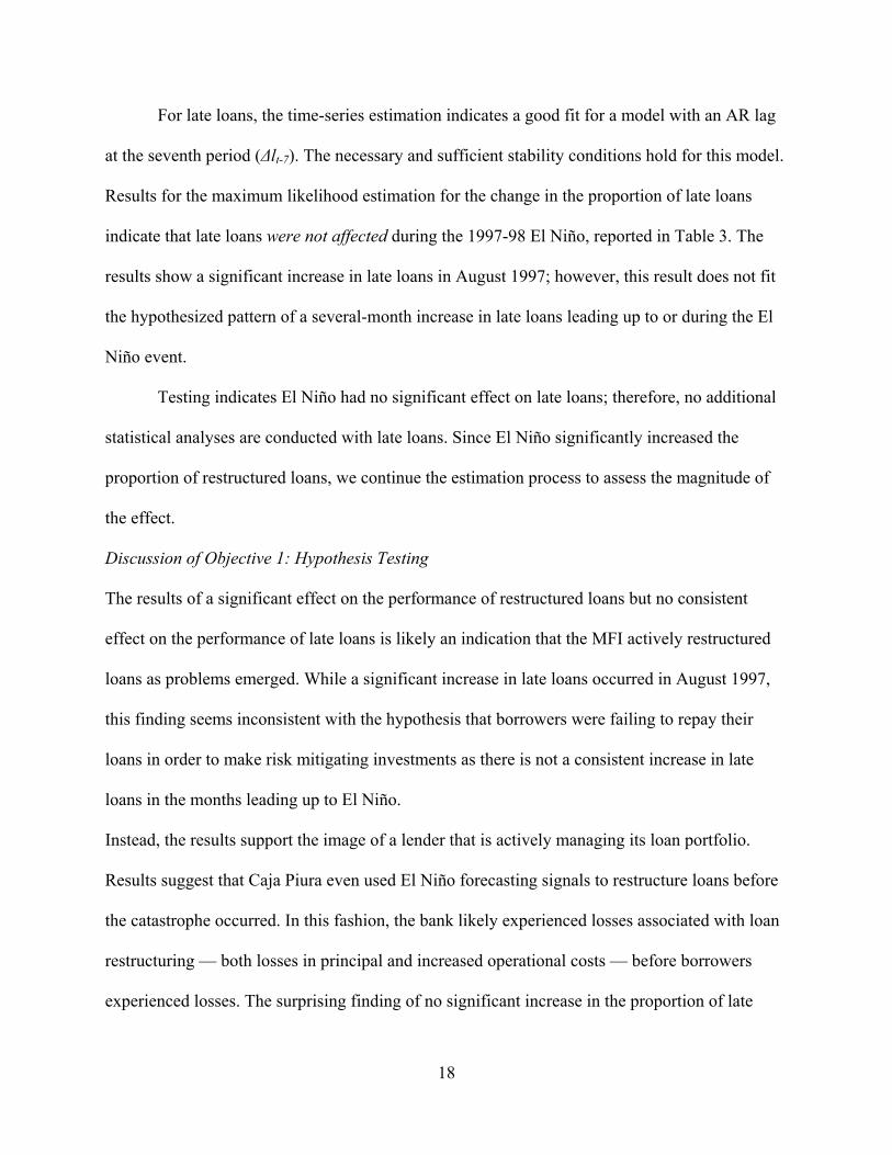
For late loans, the time-series estimation indicates a good fit for a model with an AR lag

at the seventh period (Δlt-7). The necessary and sufficient stability conditions hold for this model.

Results for the maximum likelihood estimation for the change in the proportion of late loans

indicate that late loans were not affected during the 1997-98 El Niño, reported in Table 3. The

results show a significant increase in late loans in August 1997; however, this result does not fit

the hypothesized pattern of a several-month increase in late loans leading up to or during the El

Niño event.

Testing indicates El Niño had no significant effect on late loans; therefore, no additional

statistical analyses are conducted with late loans. Since El Niño significantly increased the

proportion of restructured loans, we continue the estimation process to assess the magnitude of

the effect.

Discussion of Objective 1: Hypothesis Testing

The results of a significant effect on the performance of restructured loans but no consistent

effect on the performance of late loans is likely an indication that the MFI actively restructured

loans as problems emerged. While a significant increase in late loans occurred in August 1997,

this finding seems inconsistent with the hypothesis that borrowers were failing to repay their

loans in order to make risk mitigating investments as there is not a consistent increase in late

loans in the months leading up to El Niño.

Instead, the results support the image of a lender that is actively managing its loan portfolio.

Results suggest that Caja Piura even used El Niño forecasting signals to restructure loans before

the catastrophe occurred. In this fashion, the bank likely experienced losses associated with loan

restructuring — both losses in principal and increased operational costs — before borrowers

experienced losses. The surprising finding of no significant increase in the proportion of late

19

loans before, during, or after the event also supports the conclusion that the bank had a strong

preference for restructuring loans rather than increasing its portfolio of late loans and was

working dynamically to minimize losses as problems emerged. The lender might be motivated to

take this strategy due to higher provisioning rates for late loans than restructured loans or as a

means to encourage borrowers to continue paying rather than defaulting as their capacity to pay

changed.

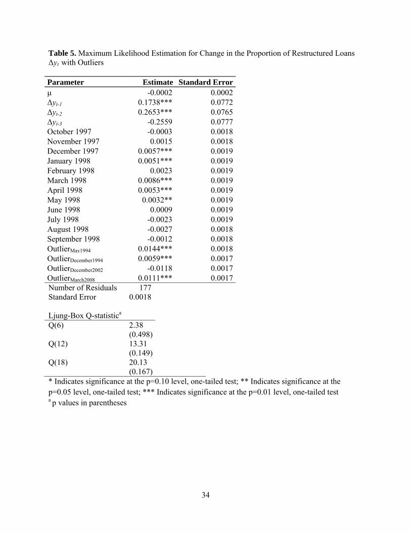
Estimating the Magnitude of the Effect

To improve estimation of the magnitude of the effect, the four most significant outliers — May

1994, December 1994, December 2002, and March 2008 — are added as dummy variables to the

model to improve fit Excluding values associated with the 1997-98 El Niño, these outliers

represent the most extreme changes from one period to the next. We do not know the specific

events that occurred during these months to cause such significant changes in the proportion of

restructured loans.

The time-series process was again tested and several autoregressive structures were

compared. The analyses indicated no MA terms should be included, but that two AR models —

one AR model for periods = 1, 2, 3, and7 and one AR model for periods = 1, 2, and3 —

are suitable according to ACF and PACF residuals and the goodness of fit and white noise

measures, shown in Table 4. Because these models are comparable, the AR model with lags at 1,

2, and 3 is chosen for parsimony. Thus, the model isΔ = + + + + + +

The necessary and sufficient conditions for stability hold for this model.

Second, we apply the intervention analysis procedure. Given this model, we use a

maximum likelihood estimation to examine the immediate effects of El Niño on the change in

20

the proportion of restructured loans, results shown in Table 5. The immediate effect is seen in the

monthly dummy variables for those months with significant increases for the time series model

used in hypothesis testing — December 1997, January, March, April, and May 1998.. The largest

immediate effect is seen in March 1998 when the proportion of restructured loans increases by

0.86 percent of the value of the loan portfolio.

To estimate the long-term effects, we return to the dependence order of the model. The

process for estimating long-term effects for a model with a single AR term is described in the

Model and Data section. Extending the example from that section to the time-series model in this

analysis, which has three AR terms, leads to the following Δ = 1 + + +⋯+ + + +⋯+ + + +⋯+

where represents the dummy for each of the months (e.g., March 1998) and the jth

superscript represents the final value of included for which is arbitrarily close to zero —

this term converges to zero at an exponential rate as increases. The term converges to zero

after roughly 10 periods for this El Niño event based on the coefficients in the model. To identify

the entire effect of El Niño on the change in proportion of restructured loans, the long-term

effects for all significant months must be added together, shown in Table 6.5 These analyses

indicate El Niño had a total cumulative effect of 3.8 percent, that is, the proportion of

restructured loans increased by 3.8 percent of the value of the total loan portfolio due to the

1997-98 El Niño.

Discussion of Objective 2: Estimating the Effect of El Niño

The total estimated increase in the proportion of restructured loans at a level of 3.8 percent of the

5 Confidence intervals are also included in Table 5 to assist the reader in evaluating the precision with which the immediate effects are evaluated.

21

total portfolio represents the highest magnitude effect of the 1997-98 El Niño event when

examining the loan portfolio. That is, the lender would have experienced a permanent 660

percent increase in restructured loans if the loans never matured and the bank took no further

action to minimize losses.6 The actual proportion of restructured loans fails to reach this

magnitude most likely because of actions taken by the lender to stem losses. As can be seen in

Figure 2, the proportion of restructured loans declined following the event, perhaps due to debt-

forgiveness policies of the bank, but for several years, the bank maintained a higher proportion

of restructured loans than before the event.

Conclusions and Policy Implications

This study uses time-series estimation and intervention analysis to test and estimate the effects of

the 1997-98 El Niño on loan portfolio performance for a rural lender in Peru. The event

significantly increased the proportion of restructured loans but did not increase the proportion of

late loans in the portfolio. The total effect of El Niño was estimated as an increase in restructured

loans of 3.8 percent of the total value of the loan portfolio. The largest single immediate effect

for restructured loans occurred in March 1998 when the increase was equivalent to 0.86 percent

of the lending portfolio.

The immediate and total effects of the 1997-98 El Niño event are dramatic. The average

proportion of restructured loans from January 1994 to November 1997 was 0.5 percent,

indicating the event increased the proportion of restructured loans 660 percent above the average

value. Given that the value of the total loan portfolio before the event in November 1997 was

54.6 million Peruvian Nuevo Soles (PEN), the estimated total value of loans restructured due to

6 Using the differenced data, which is required for this time-series to be stationary, necessitates conceptualizing the change due to the El Niño event as permanent. The analyses do not provide any indication as to how quickly the lender can recover from the event. Evaluating lender recovery requires information about bank policies (average loan maturity for restructured loans, the extent to which loans were forgiven, etc.), bank liabilities (e.g., savings deposits), and systemic events such as political interventions, which is beyond the scope of this paper.

22

the 1997-98 El Niño was PEN 2.1 million, roughly USD 771,000 (in 1997 dollars).7

These analyses demonstrate three primary themes regarding loan portfolio performance

and natural disaster risk. First, the correlated risk exposure of many small borrowers can lead to

large effects in the lending portfolio when a catastrophic event occurs. This finding is not new

and is consistent with the emphasis of the Basel Committee on the interrelatedness of operational

and credit risks; however, this case is a dramatic example of this exposure. These findings are

worthy of careful consideration by regulators managing MFIs as they may challenge the

sufficiency of generally accepted operational risk assessment approaches in some contexts. For

example in Peru, Caja Piura and similar MFIs are regulated under standards quite similar to

Basel II (see Superintendencia de Banca, Seguros y AFP, 2009). Under these regulations MFIs

hold capital to manage their operational risk based on a percentage of their annual positive gross

income from the previous three years.8 Estimating operational risk based on gross income levels

may be insufficient for banks concentrated in regions exposed to significant natural disaster risk.

We recognize many MFIs are not under ongoing regulatory supervision, and for these

institutions prudent consideration on the part of owners and managers is needed.

In practice, such catastrophic events have led some microcredit providers to ration credit,

especially for agriculture which can be one of the economic sectors most highly exposed to the

correlated risks that are tied to natural disasters. Caja Piura began rationing credit to agriculture

after the 1997-98 El Niño (Tarazona and Trivelli, 2006). While limiting exposure to correlated

risk through credit rationing is an understandable approach for lenders, it can both impede

growth for the bank and development in the region (Boucher et al., 2008). It is also worth noting

7 The exchange rate in the fall of 1997 was 2.66 PEN to 1 USD (United States Central Intelligence Agency, 2002). 8 Two approaches under Basel II require basing capital requirements for operational risk on gross income: the Standardized Approach and the Basic Indicator Approach (BCBSm 2004). There a more advanced approach for managing operational risk, but as of January 2010, the Peruvian banking regulator reported no banks use the most advanced approach in Peru.

23

again the significant infrastructure and household income losses that had widespread effects in

Piura extending beyond agriculture (Oft, 2009). Such reports of widespread losses challenge the

effectiveness of agricultural credit rationing strategies for MFIs in this region, as well. More

efficient and effective risk management mechanisms such as those that transfer these risks

through insurance or securitization have the potential to greatly improve the performance of

microcredit providers.

Second, the findings emphasize the importance of considering bank management in

assessing disaster risk to a loan portfolio. A theme from the diverse intervention analysis and

event studies literatures is that the effects of natural disasters are often context-specific.

Likewise, many factors determine the way banks optimize portfolio performance that are based

on the risk, local institutions, culture, and available disaster relief mechanisms. Perhaps the most

fascinating aspect of the analyses in this study is the evidence that Caja Piura likely used

forecasting information to restructure loans before significant losses occurred.

Third, the findings imply that bank strategies to minimize losses may require long-term

restructuring that perpetuates the effects of the disaster in the community. These analyses show

that Caja Piura restructured nearly all the loans affected by El Niño, and reports from the region

indicate that the terms of restructuring included extending the loan years into the future

(Tarazona and Trivelli, 2006). Not only do such repayment plans create long-term indebtedness

among local borrowers, but they tie up bank capital that could otherwise be used to expand

access to credit. Findings in other regions of the world indicate these long-term consequences to

the community are common among other types of disasters, as well (Dercon, 1998;

GlobalAgRisk, 2009). Thus, bank policies combined with risk transfer mechanisms, perhaps risk

transfer mechanisms for borrowers, that offer credible alternatives to long-term loan

24

restructuring have the potential to improve recovery time for the community or region. Careful

consideration is needed to develop clear ex ante rules for these policies as ad hoc debt

forgiveness can entrench borrower expectations of nonrepayment that contribute to longer term

credit constraints.

Important follow-up analyses could advance this work. “Natural disasters” encompasses

a broad category of events and El Niño probably poorly represents some types of disasters. For

example, the effects of drought may not be as pervasive as flooding as it is not likely to

destroying transportation infrastructure, homes, or buildings. Thus, these methods could be

replicated for lenders that have experienced other disasters, which may lead to problem loans and

the need for restructuring. Additionally, each occurrence of the same natural disaster can have

significantly different effects (Jobst, 2007); therefore, comparing these findings to analyses using

data for previous extreme El Niño events, such as the one in 1982-83, may be insightful.

25

References

Armendáriz, B. and Morduch, J. (2010), “Subsidy and sustainability”, in The Economics of

Microfinance, 2nd ed., MIT Press, Cambridge, MA, pp. 231-256.

Basel Committee on Banking Supervision (2004), International Convergence of Capital

Measurement and Capital Standards: A Revised Framework, Bank for International Settlements,

Basel, Switzerland.

Bessis, J. (1998), “Correlations and portfolio risk”, in Risk Management in Banking, John Wiley

& Sons, New York, NY, pp. 289-297.

Binder, J.J. (1998), “The event study methodology since 1969”, Review of Quantitative Finance

and Accounting, Vol. 11 No. 2, pp. 111-137.

Box, G.E.P. and Jenkins, G.M. (1968), “Some recent advances in forecasting and control”,

Journal of the Royal Statistical Society. Series C (Applied Statistics), Vol. 17 No. 2, pp. 91-109.

Boucher, S., Carter, M. and Guirkinger, C. (2008), “Risk rationing and wealth effects in credit

markets: theory and implications for agricultural development”, American Journal of

Agricultural Economics, Vol. 90 No. 2, pp. 409-423.

Charnobai, A. and Rachev, S.T. (2006), “Applying robust methods to operational risk

modeling”, Journal of Operational Risk, Vol. 1 No. 1, pp. 27-41.

Cruzado Silveri, E. (1999), “El fenómeno El Niño en Piura 97/98 y el rol del estado:

consecuencias sectoriales y sociales 7”, report, Centro de Investigacion y Promocion del

Campesinado (CIPCA), Departamento de Investigacion Socioeconomica, Piura, Peru.

26

Dercon, S. (1998), “Wealth, risk, and activity choice: cattle in western Tanzania”, Journal of

Development Economics, Vol. 55 No.1, pp. 1-42.

Enders, W. (2004), Applied Econometric Time-Series, 2nd ed., John Wiley & Sons, Hoboken, NJ.

Fox, R.T. (1996), “Using intervention analysis to assess catastrophic events on business

environment”, International Advances in Economic Research, Vol. 2 No. 3, pp. 341-349.

Garside, T., Stott, H. and Stevens, A. (1999),“Credit portfolio management”, available at:

http://www.erisk.com/learning/research/013_200creditportfoliomodels.pdf (accessed 23 April

2010).

GlobalAgRisk (2009), The Role of Risk Assessment in Setting Insurance Priorities and Policy,

Vol. 2, Developing Agricultural Insurance in Vietnam: Four Educational Handbooks, AgroInfo,

Hanoi, Vietnam.

Greene, W.H. (2000), Econometric Analysis, 4th ed., Prentice Hall, Upper Saddle River, NJ.

Greuning, H. and Bratanovic, S.B. (2009), Analyzing Banking Risk: A Framework for Assessing

Corporate Governance and Risk Management, 3rd ed., The World Bank, Washington, DC.

Guzhva, V.S. (2008), “Applying intervention analysis to financial performance data: the case of

US airlines and September 11th”, Journal of Economics and Finance, Vol. 32 No. 3, pp. 243-

259.

Hultkrantz, L. and Olsson, K. (1997), “Chernobyl effects on domestic and inbound tourism in

Sweden—a time-series analysis”, Environmental and Resource Economics, Vol. 9 No. 2, pp.

239-258.

27

Instituto Nacional de Estadística e Informática (2007), “Perú: perfil de la pobreza según

departamentos, 2004–2006”, report REF HC 230.P6 I51P, Instituto Nacional de Estadística e

Informática, Lima, Peru, December.

Jobst, A. (2007), “Operational risk: the sting is still in the tail but the poison depends on the

dose”, working paper WP/07/239, International Monetary Fund, Washington, DC, November.

Katchova, A. and Barry, P. (2005), “Credit risk models and agricultural lending”, American

Journal of Agricultural Economics, Vol. 87 No. 1, pp. 194-205.

MacKinlay, A.C. (1997), “Event studies in economics and finance”, Journal of Economic

Literature, Vol. 35 No. 1, pp. 13-39.

McPhaden, M.J. (2003), “El Niño and La Niña: causes and global consequences”, in

MacCracken, M.C. and Perry, J.S. (Eds.), Encyclopedia of Global Environmental Change,

Volume 1, The Earth System: Physical and Chemical Dimensions of Global Environmental

Change, John Wiley & Sons, Hoboken, NJ, pp. 353-370.

Prestemon, J.P. and Holmes, T.P. (2000), “Timber price dynamics following a natural

catastrophe”, American Journal of Agricultural Economics, Vol. 82 No. 1, pp. 145-160.

Philippatos, G.C. and Viswanathan, K.G. (1991), “Brazilian debt crisis and financial markets: an

analysis of major economic events leading to the Brazilian debt moratorium”, Applied Financial

Economics, Vol. 1 No. 4, pp. 223-234.

Pindyck, R.S. and Rubinfeld, D.L. (1997), Econometric Models and Economic Forecasts, 4th ed.,

McGraw-Hill, New York, NY.

28

Oft, P. (2009), “Can resilience be built through microfinance tools? A case study of coping and

adaptation strategies to climate-related shocks in Piura, Peru”, PhD dissertation, University of

Bonn, Germany, March.

Oldenborgh, G.J., Philip, S.Y. and Collins, M. (2005), “El Niño in a changing climate: a multi-

model study”, Ocean Science, Vol. 1 No. 2, pp. 81-95.

Orlove, B.S., Broad, K. and Petty, A.M. (2004), “Factors that influence the use of climate

forecasts: evidence from the 1997/98 El Niño event in Peru”, American Meteorological Society,

Vol. 85 No. 11, pp. 1735-1743.

Superintendencia de Banca, Seguros y AFP (2009), “Resolución S.B.S. N°2115-2009,

Reglamento para el requerimiento de patrimonio efectivo por riesgo operacional”,

Superintendencia de Banca, Seguros y AFP, Lima, Perú, 2 April.

Superintendencia de Banca, Seguros y AFP (2008), “Resolution 11356-2008, Se aprueba el

nuevo reglamento para la evaluación y clasificación del deudor y la exigencia de provisiones”,

Superintendencia de Banca, Seguros y AFP, Lima, Perú, 19 November.

Skees, J.R. and Barnett, B.J. (2006), “Enhancing micro finance using index-based risk transfer

products”, Agricultural Finance Review, Vol. 66 No. 2, pp. 235-250.

Skees, J.R. and Murhpy, A.G. (2009) “ENSO Business Interruption Index Insurance (EBIII) for

catastrophic flooding in Piura, Peru”, working paper, GlobalAgRisk, Inc., Lexington, KY, 12

February.

Tarazona, A. and Trivelli, C. (2006), “Financiamento rural en Piura: informe final”, final report,

29

Instituto de Estudios Peruanos, Lima, Peru, January.

Trivelli, C. (2006), “Rural finance and insurance on the north coast of Peru”, summary report

2005/06, Instituto de Estudios Peruanos, Lima, Peru, September.

United States Agency for International Development (2006), “Hedging weather risk for

microfinance institutions in Peru: comprehensive report”, report prepared by GlobalAgRisk, Inc.,

United States Agency for International Development, Washington, DC, November.

United States Central Intelligence Agency (2002), “Field listing—Exchange rates, The World

Factbook 2002”, available at: http://www.faqs.org/docs/factbook/fields/2076.html (accessed 23

April 2010).

Worthington, A. and Valadkhani, A. (2004), “Measuring the impact of natural disasters on

capital markets: an empirical application using intervention analysis”, Applied Economics, Vol.

36 No. 19, pp. 2177-2186.

30

Table 1. Summary Statistics and the Augmented Dickey-Fuller Test for the Proportion of Restructured Loans and Late Loans Proportion of

Restructured Loans

yt

Change in Proportion of Restructured

Loans Δyt

Proportion of Late Loans

lt

Change in Proportion of Late Loans

Δlt

Observations 178 177 178 177 Mean 0.0151 0.0001 0.0595 -0.0002 Standard deviation

0.0090 0.0027 0.0135 0.0051

Maximum 0.0351 0.0137 0.1142 0.0262 Minimum 0.0004 -0.0125 0.0262 -0.0237 ADF statistics F F F F Constant Only 2.40 72.90*** 4.57* 90.24*** (0.460)a (0.001) (0.053) (0.001) Constant and Trend

2.45 72.64*** 4.96 90.02***

(0.688) (0.001) (0.185) (0.001) *** indicates significance at the p=0.01 level a p values in parentheses

31

Table 2. Maximum Likelihood Estimation for Change in the Proportion of Restructured Loans Δyt , One-Tailed Test Parameter Estimate Standard Errorμ -0.0001 0.0002Δyt-3 -0.1975 0.0751Δyt-7 0.2230*** 0.0755October 1997 0.0000 0.0025November 1997 0.0014 0.0025December 1997 0.0057*** 0.0024January 1998 0.0046** 0.0025February 1998 0.0018 0.0025March 1998 0.0089*** 0.0024April 1998 0.0052** 0.0024May 1998 0.0044** 0.0025June 1998 0.0006 0.0025July 1998 -0.0015 0.0024August 1998 -0.0049 0.0025September 1998 -0.0015 0.0025Number of Residuals 177 Standard Error 0.002454 Ljung-Box Q-statistica

Q(6) 8.59 (0.072)

Q(12) 10.39 (0.407)

Q(18) 11.18 (0.798)

* Indicates significance at the p=0.10 level, one-tailed test; ** Indicates significance at the p=0.05 level, one-tailed test; *** Indicates significance at the p=0.01 level, one-tailed test a p values in parentheses

32

Table 3. Maximum Likelihood Estimation for Changes in Proportion of Late Loans Δlt Parameter Estimate Standard Errorμ -0.0003 0.0003Δlt-7 -0.2722 0.0768June 1997 -0.0004 0.0050July 1997 0.0040 0.0050August 1997 0.0094* 0.0050September 1997 0.0016 0.0050October 1997 0.0062 0.0050November 1997 -0.0015 0.0050December 1997 -0.0161 0.0050January 1998 0.0052 0.0051February 1998 0.0040 0.0051March 1998 0.0003 0.0050April 1998 0.0042 0.0050May 1998 -0.0064 0.0050June 1998 0.0008 0.0050July 1998 0.0006 0.0050August 1998 0.0041 0.0050September 1998 -0.0002 0.0050Number of Residuals 177 Standard Error 0.0050

* Indicates significance at the p=0.10 level, one-tailed test a p values are in parentheses

Ljung-Box Q-statistica Q(6) 3.41

(0.636) Q(12) 5.59

(0.899) Q(18) 17.66

(0.411)

33

Table 4. Comparison of ARIMA Models for Change in the Proportion of Restructured Loans Δyt

AR structures Model with AR lags

p=1, 2, 3, 7 Model with AR lags p=1,2,3

Estimates of lag coefficientsa μ -0.0002 -0.0002 (-0.92) (-0.93) Δ 0.162**

(2.21) 0.16027** (2.05) Δ 0.290***

(3.95) 0.26407*** (3.42) Δ -0.256***

(-3.46) -0.25171*** (-3.21) Δ 0.270***

(3.78)

Goodness of Fit Measures Standard Error Estimate 0.001727 0.001797 AIC -1728.97 -1713.95 SBC -1662.27 -1640.9 Ljung-Box Q-statisticb Q(6) 3.48

(0.176) 2.38 (0.498)

Q(12) 6.30 (0.613)

13.31 (0.149)

Q(18) 10.96 (0.690)

20.13 (0.167)

* Indicates significance at the p=0.10 level ** Indicates significance at the p=0.05 level *** Indicates significance at the p=0.01 level

a t values are in parentheses b p values are in parentheses

34

Table 5. Maximum Likelihood Estimation for Change in the Proportion of Restructured Loans Δyt with Outliers Parameter Estimate Standard Errorμ -0.0002 0.0002Δyt-1 0.1738*** 0.0772Δyt-2 0.2653*** 0.0765Δyt-3 -0.2559 0.0777October 1997 -0.0003 0.0018November 1997 0.0015 0.0018December 1997 0.0057*** 0.0019January 1998 0.0051*** 0.0019February 1998 0.0023 0.0019March 1998 0.0086*** 0.0019April 1998 0.0053*** 0.0019May 1998 0.0032** 0.0019June 1998 0.0009 0.0019July 1998 -0.0023 0.0019August 1998 -0.0027 0.0018September 1998 -0.0012 0.0018OutlierMay1994 0.0144*** 0.0018OutlierDecember1994 0.0059*** 0.0017OutlierDecember2002 -0.0118 0.0017OutlierMarch2008 0.0111*** 0.0017Number of Residuals 177 Standard Error 0.0018 Ljung-Box Q-statistica

Q(6) 2.38 (0.498)

Q(12) 13.31 (0.149)

Q(18) 20.13 (0.167)

* Indicates significance at the p=0.10 level, one-tailed test; ** Indicates significance at the p=0.05 level, one-tailed test; *** Indicates significance at the p=0.01 level, one-tailed test a p values in parentheses

35

Table 6 Immediate and Total Effects on the Change in Proportion of Restructured Loans of the 1998 El Niño by Month

Month Immediate Effect c (%)

95% Confidence Intervals c (one-tailed test, %)9

Total Effect (%)

December 1997 0.57 0.22-0.88 0.78 January 1998 0.51 0.20-0.82 0.70 March 1998 0.86 0.55-1.17 1.17 April 1998 0.53 0.22-0.84 0.72May 1998 0.32 0.01-0.63 0.44Cumulative Total Effect 3.81

9 0.95 = ( − 1.64 ∗ ≤ ≤ + 1.64 ∗ ) where c is the effect in the sample, C is the actual effect, and se is the standard error of the estimate

36

Figure 1. Effects of Correlated Risk on the Lending Portfolio

37

Figure 2. Proportion of Restructured Loans by Month from January 1994 to October 2008

38

Figure 3. Proportion of Late Loans by Month from January 1994 to October 2008