Embed Size (px)
Citation preview

LMM and GLMM basics
©2011 Ben Bolker
March 14, 2011
Licensed under the Creative Commons attribution-noncommercial
license (http://creativecommons.org/licenses/by-nc/3.0/). Please
share & remix noncommercially, mentioning its origin.
1 Preliminaries
> library(faraway)
> data(pulp)
You should always examine the data. If you are worried about datasnooping, then make sure that you decide beforehand (and if necessary writedown) which analyses you plan do to, and why. Proceeding with analysiswithout doing at least cursory textual and graphical summaries of the datais insane.
1.1 Textual summaries
> summary(pulp)
bright operator
Min. :59.80 a:5
1st Qu.:60.00 b:5
Median :60.50 c:5
Mean :60.40 d:5
3rd Qu.:60.73
Max. :61.00
From this we can see that the data set is extremely simple (a singlenumerical response and a single categorical predictor). The number of op-erators is so small that we can immediately see the experimental design(5 measurements for each of 4 operators), but if necessary we could use
1

1 PRELIMINARIES 2
> table(pulp$operator)
to get a full enumeration of the number of observations per operator (in thiscase, we could also increase the value of maxsum (default 7), which speci-fies how many levels of factors to report, e.g. summary(pulp,maxsum=10):see ?summary.data.frame). For more complicated data sets, table is re-ally useful for figuring out the experimental design: how treatments aredistributed among blocks, whether the design is balanced, etc..
We could go slightly further in getting summaries:
> tmpf <- function(x) { round(c(mean(x),sd(x)),3) }
> aggregate(bright~operator,data=pulp,FUN=tmpf)
operator bright.1 bright.2
1 a 60.240 0.518
2 b 60.060 0.241
3 c 60.620 0.228
4 d 60.680 0.217
The command stem(pulp$bright) gives a text-based approximation ofa histogram of the data (something of an anachronism at this point, butcute).
1.2 Graphical summaries
At this point it really makes much more sense to turn to graphical sum-maries.
Try
> with(pulp,plot(operator,bright))
to see what you get. Were you surprised? Why is this form of plottingsuboptimal for a data set with only 5 observations per group, even thoughit would make sense for a larger data set . . . ? You could add the individualpoints to the plot:
> with(pulp,points(operator,bright,col="red"))
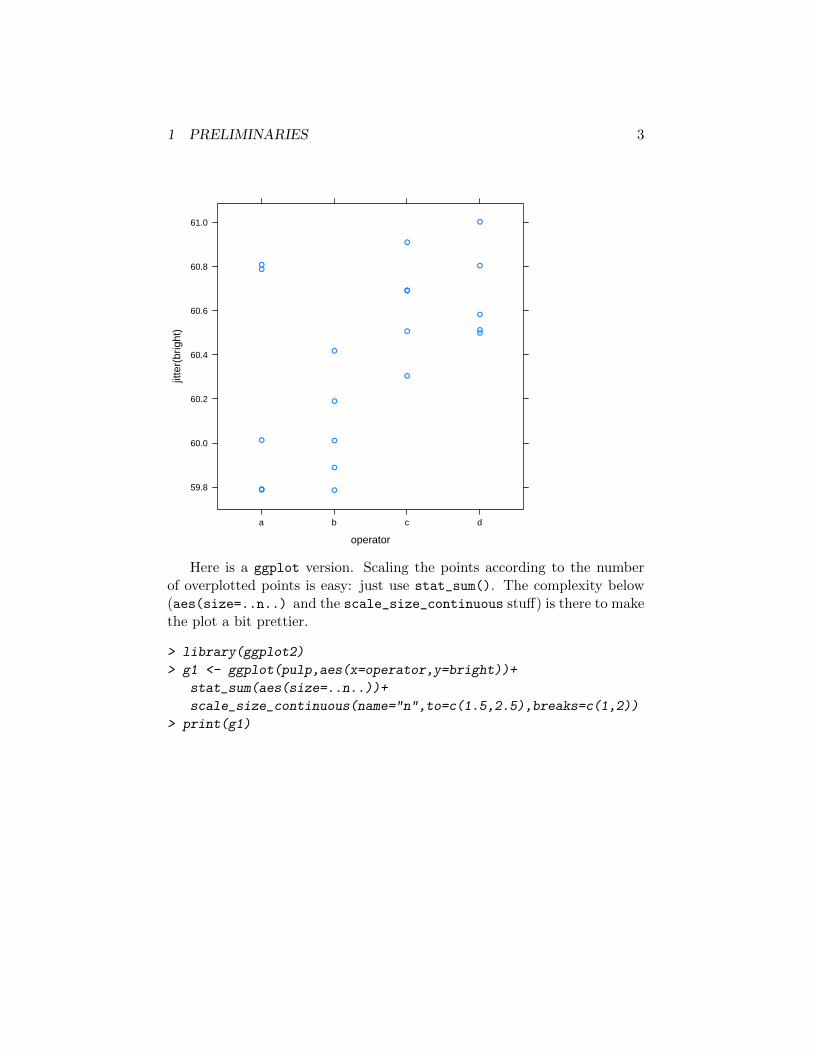
By now you should have noticed that some points have duplicated nu-merical values. The quick and dirty way to deal with this is to jitter thedata, e.g.:
> library(lattice)
> print(xyplot(jitter(bright)~operator,data=pulp))
1 PRELIMINARIES 3
operator
jitte
r(br
ight
)
59.8
60.0
60.2
60.4
60.6
60.8
61.0
a b c d
●
●
●●
● ●
●
●
●
●
●●
●
●
●
●
●
●
●●
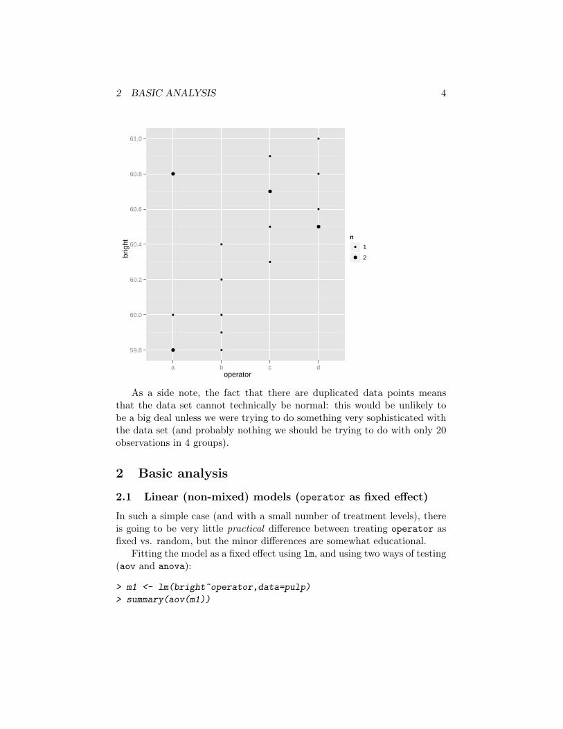
Here is a ggplot version. Scaling the points according to the numberof overplotted points is easy: just use stat_sum(). The complexity below(aes(size=..n..) and the scale_size_continuous stuff) is there to makethe plot a bit prettier.
> library(ggplot2)
> g1 <- ggplot(pulp,aes(x=operator,y=bright))+
stat_sum(aes(size=..n..))+
scale_size_continuous(name="n",to=c(1.5,2.5),breaks=c(1,2))
> print(g1)
2 BASIC ANALYSIS 4
operator
brig
ht
59.8
60.0
60.2
60.4
60.6
60.8
61.0
●
●
●
●
●
●
●
●
●
●
●
●
●
●
●
●
a b c d
n● 1
● 2
As a side note, the fact that there are duplicated data points meansthat the data set cannot technically be normal: this would be unlikely tobe a big deal unless we were trying to do something very sophisticated withthe data set (and probably nothing we should be trying to do with only 20observations in 4 groups).
2 Basic analysis
2.1 Linear (non-mixed) models (operator as fixed effect)
In such a simple case (and with a small number of treatment levels), thereis going to be very little practical difference between treating operator asfixed vs. random, but the minor differences are somewhat educational.
Fitting the model as a fixed effect using lm, and using two ways of testing(aov and anova):
> m1 <- lm(bright~operator,data=pulp)
> summary(aov(m1))

2 BASIC ANALYSIS 5
Df Sum Sq Mean Sq F value Pr(>F)
operator 3 1.34 0.44667 4.2039 0.02261 *
Residuals 16 1.70 0.10625
---
Signif. codes: 0 ‘***’ 0.001 ‘**’ 0.01 ‘*’ 0.05 ‘.’ 0.1 ‘ ’ 1
> anova(m1)
Analysis of Variance Table
Response: bright
Df Sum Sq Mean Sq F value Pr(>F)
operator 3 1.34 0.44667 4.2039 0.02261 *
Residuals 16 1.70 0.10625
---
Signif. codes: 0 ‘***’ 0.001 ‘**’ 0.01 ‘*’ 0.05 ‘.’ 0.1 ‘ ’ 1
We can also use anova to explicitly test one model against its reducedversion (again with the same results):
> m0 <- update(m1,.~.-operator)
> anova(m0,m1)
Analysis of Variance Table
Model 1: bright ~ 1
Model 2: bright ~ operator
Res.Df RSS Df Sum of Sq F Pr(>F)
1 19 3.04
2 16 1.70 3 1.34 4.2039 0.02261 *
---
Signif. codes: 0 ‘***’ 0.001 ‘**’ 0.01 ‘*’ 0.05 ‘.’ 0.1 ‘ ’ 1
2.2 Classical approach: operator as a random effect
The aov() function allows a simple form of random effects estimation, viathe Error specification:
> a1 <- aov(bright~Error(operator),data=pulp)
> (s1 <- summary(a1))

2 BASIC ANALYSIS 6
Error: operator
Df Sum Sq Mean Sq F value Pr(>F)
Residuals 3 1.34 0.44667
Error: Within
Df Sum Sq Mean Sq F value Pr(>F)
Residuals 16 1.7 0.10625
(We could also have expressed the formula as an “intercept-only” model viabright~1+Error(operator).) There are no fixed effects at all in this model,so the summary shows only the error SSQ and MSQ.
We can (not particularly conveniently) test the hypothesis that theamong-operator variance is zero by using pf(...,lower.tail=FALSE) tocompute the appropriate upper tail area:
> pf(0.44667/0.10625,df1=3,df2=16,lower.tail=FALSE)
[1] 0.02260834
In this case the p-values are identical whether we treat operator as a randomor a fixed effect . . .
I did the test above by looking at the results from summary and pluggingthe appropriate numbers into pf. As a general practice, it is better to specifythis test based on digging the values out from inside the s1 object, but this isactually a tremendous nuisance because of the way the results are organizedinternally: it takes quite a bit of digging around with str to figure out whatto extract.
> ssq_operator <- s1[["Error: operator"]][[1]][["Mean Sq"]]
> ssq_within <- s1[["Error: Within"]][[1]][["Mean Sq"]]
> df_operator <- s1[["Error: operator"]][[1]][["Df"]]
> df_within <- s1[["Error: Within"]][[1]][["Df"]]
> pf(ssq_operator/ssq_within,df_operator,df_within,lower.tail=FALSE)
[1] 0.02260890
The bottom line is that, while you can do ANOVA on classical balanceddesigns in R (see MASS chapter 10 for more details), it is not very convenientto do so.
In particular, the classical machinery provided by R is not well gearedto doing F tests of random effects; most of the testing framework assumes

2 BASIC ANALYSIS 7
that you want to test particular fixed effects with appropriate error terms.(My guess about this omission is that, in the classical experimental designframework, the random effect terms (e.g. experimental block) are all nui-sance variables that are neither of interest in themselves nor dispensableif they turn out to be non-significant. In contrast, in genetics — the otherhistorical source of random and mixed effects ANOVA — the random effectsare of great interest . . . )
2.3 Using lme
Rule of thumb: if you have a design that is more than slightly complicated(e.g. unbalanced, non-nested, etc.), then you should use lme (nlme package)or lmer (lme4 package).
> library(nlme)
> m2 <- lme(bright~1,random=~1|operator,data=pulp)
> summary(m2)
Linear mixed-effects model fit by REML
Data: pulp
AIC BIC logLik
24.6262 27.45952 -9.3131
Random effects:
Formula: ~1 | operator
(Intercept) Residual
StdDev: 0.2609286 0.32596
Fixed effects: bright ~ 1
Value Std.Error DF t-value p-value
(Intercept) 60.4 0.1494437 16 404.1655 0
Standardized Within-Group Residuals:
Min Q1 Med Q3 Max
-1.4666202 -0.7595239 -0.1243466 0.6280955 1.6012410
Number of Observations: 20
Number of Groups: 4
The summary extracts summary statistics about the fit (AIC, BIC, and log-likelihood); standard deviations (and correlations in more complex cases)

2 BASIC ANALYSIS 8
for each random effect fitted and for the residual standard error; a standardtable of fixed-effect parameters with the value, standard error, and Waldstatistics (and p values); a summary of residuals (good for a preliminaryassessment of whether the residuals are badly skewed or otherwise wonky);and basic statistics on the number of levels per group (also good for sanity-checking your results).
The standard accessors (fitted, residuals, logLik, AIC, predict etc.)work for lme models, with some wrinkles (for each method, see the appropri-ate lme-specific help page, e.g. ?fitted.lme for fitted, to see specificallywhat it does when applied to lme objects). There are a few accessors whichare new or different.
� use VarCorr() to extract the variance components
� coef() gives the predicted coefficients for each random-effects level:use fixef() to get just the fixed-effect coefficients or ranef() to getthe random-effects coefficients (predictors)
� lme uses the (idiosyncratic) intervals(), rather than the morestandard confint(), to extract confidence intervals (based onquadratic approximations, which are exactly correct for the fixed ef-fects but can be dicey for random-effects variances. (Use inter-
vals(...,which="fixed") or intervals(...,which="var-cov") toget just one type of intervals.)
Exercise: Try out these accessors on the model fit above. Convinceyourself that (1) the residual variance is the same as estimated above by theclassical approach; (2) that the estimated variance among operators is notthe same; (3) that the classical estimate of the among-operator variance iswithin the 95% confidence intervals estimated by lme.
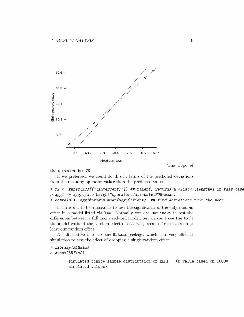
Now let’s use ranef to demonstrate the shrinkage of the estimates (pre-dictions) of operator effects:
> shrinkest <- coef(m2)[["(Intercept)"]]
> fixest <- coef(lm(bright~operator-1,data=pulp))
> par(las=1,bty="l")
> plot(shrinkest~fixest,xlab="Fixed estimates",ylab="Shrinkage estimates")
> abline(a=0,b=1)
> refit2 <- lm(shrinkest~fixest)
> abline(refit2,lty=2)
2 BASIC ANALYSIS 9
●
●
●
●
60.1 60.2 60.3 60.4 60.5 60.6 60.7
60.2
60.3
60.4
60.5
60.6
Fixed estimates
Shr
inka
ge e
stim
ates
The slope ofthe regression is 0.76.
If we preferred, we could do this in terms of the predicted deviationsfrom the mean by operator rather than the predicted values:
> r2 <- ranef(m2)[["(Intercept)"]] ## ranef() returns a *list* (length=1 in this case)
> agg1 <- aggregate(bright~operator,data=pulp,FUN=mean)
> estvals <- agg1$bright-mean(agg1$bright) ## find deviations from the mean
It turns out to be a nuisance to test the significance of the only randomeffect in a model fitted via lme. Normally you can use anova to test thedifferences between a full and a reduced model, but we can’t use lme to fitthe model without the random effect of observer, because lme insists on atleast one random effect.
An alternative is to use the RLRsim package, which uses very efficientsimulation to test the effect of dropping a single random effect:
> library(RLRsim)
> exactRLRT(m2)
simulated finite sample distribution of RLRT. (p-value based on 10000
simulated values)

3 LME4 10
data:
RLRT = 3.4701, p-value = 0.0241
If you run this a few times, you’ll get slightly different answers each time,but all should agree reasonably closely with the classical answer (p ≈ 0.02)above.
We can also compute the intra-class correlation (VarCorr produces aslightly complicated object, so we collapse it to a numeric vector beforetrying to manipulate it):
> vc <- VarCorr(m2)
> vcn <- as.numeric(vc)
> vcn[1]/(vcn[1]+vcn[2])
[1] 0.3905369
3 lme4
> ## unfortunately lme4 and nlme don't play nicely together.
> ## remove one before trying to use the other ...
> detach("package:nlme")
In lme4, random effects are expressed in a single formula along withfixed effects, as terms of the form (effect|group) (i.e. like the terms inthe random= argument to lme, but surrounded by parentheses).
> library(lme4)
> m3 <- lmer(bright~(1|operator),data=pulp)
> summary(m3)
Linear mixed model fit by REML
Formula: bright ~ (1 | operator)
Data: pulp
AIC BIC logLik deviance REMLdev
24.63 27.61 -9.313 16.64 18.63
Random effects:
Groups Name Variance Std.Dev.
operator (Intercept) 0.068084 0.26093
Residual 0.106250 0.32596
Number of obs: 20, groups: operator, 4

4 ARABIDOPSIS ANALYSIS 11
Fixed effects:
Estimate Std. Error t value
(Intercept) 60.4000 0.1494 404.2
This gives very similar results to lme. One of the main differences is that inthe summary, lmer does not give p values . . .
4 Arabidopsis analysis
And now for a brief exploration of a (much) more complicated data set . . .In this data set, the response variable is the number of fruits (i.e. seed
capsules) per plant. The number of fruits produced by an individual plant(the experimental unit) was hypothesized to be a function of fixed effects,including nutrient levels (low vs. high), simulated herbivory (none vs. apicalmeristem damage), region (Sweden, Netherlands, Spain), and interactionsamong these. Fruit number was also a function of random effects includingboth the population and individual genotype. Because Arabidopsis is highlyselfing, seeds of a single individual served as replicates of that individual.There were also nuisance variables, including the placement of the plantin the greenhouse, and the method used to germinate seeds. These wereestimated as fixed effects but interactions were excluded.
> dat.tf <- read.csv("Banta_TotalFruits.csv",
colClasses=c(rep("factor",8),"integer"))
> ## reorder levels
> dat.tf$amd <- factor(dat.tf$amd, levels=c("unclipped", "clipped"))
Running
> with(dat.tf, table(popu, gen))
(try it for yourself!) reveals that we have only 2–4 populations per regionand 2–3 genotypes per population. However, we also have 2–13 replicates pergenotype per treatment combination (four unique treatment combinations:2 levels of nutrients by 2 levels of simulated herbivory). Thus, even thoughthis was a reasonably large experiment (625 plants), there were a very smallnumber of replicates with which to estimate variance components, and manymore potential interactions than our data can support. Therefore, judiciousselection of model terms, based on both biology and the data, is warranted.We note that we don’t really have enough levels per random effect, nor
4 ARABIDOPSIS ANALYSIS 12
enough replication per unique treatment combination. Therefore, we decideto ignore the fixed effect of “region”, but now recognize that populations indifferent regions are widely geographically separated.
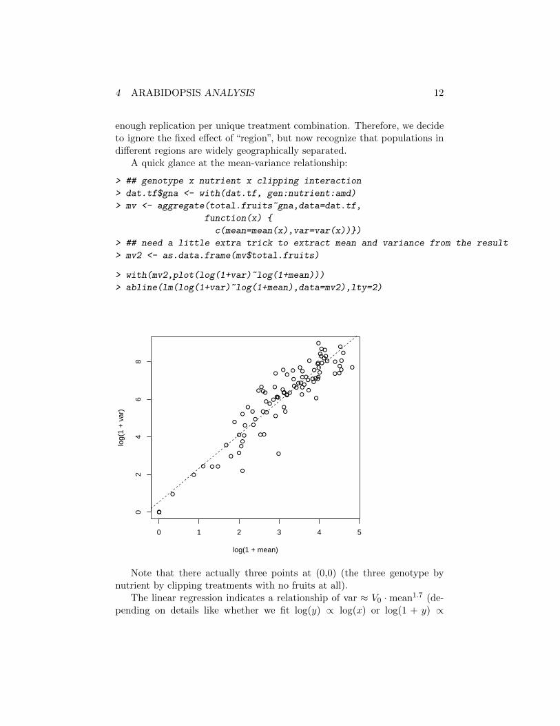
A quick glance at the mean-variance relationship:
> ## genotype x nutrient x clipping interaction
> dat.tf$gna <- with(dat.tf, gen:nutrient:amd)
> mv <- aggregate(total.fruits~gna,data=dat.tf,
function(x) {
c(mean=mean(x),var=var(x))})
> ## need a little extra trick to extract mean and variance from the result
> mv2 <- as.data.frame(mv$total.fruits)
> with(mv2,plot(log(1+var)~log(1+mean)))
> abline(lm(log(1+var)~log(1+mean),data=mv2),lty=2)
●
●
●
●
●
●
●
●●
●
●
●
●
●
●
●●
●
●
●
●
●
●
●
●
●
●
●
●
●
●
●
●
●
●
●
●
●
●
●
●
●
●
●
●
●
●
●
●
●
●
●
●
●
● ●
●
●
●
●
●
●
●
●
●
●
●
●
●
●
●●
●
●
●●
●
●
●
●
●●
●
●
●
●
●
●
●
●
●
●
●
●
●
●
0 1 2 3 4 5
02
46
8
log(1 + mean)
log(
1 +
var
)
Note that there actually three points at (0,0) (the three genotype bynutrient by clipping treatments with no fruits at all).
The linear regression indicates a relationship of var ≈ V0 ·mean1.7 (de-pending on details like whether we fit log(y) ∝ log(x) or log(1 + y) ∝

4 ARABIDOPSIS ANALYSIS 13
log(1 + x)). We will hope that adding an observation-level random effectwill take care of this overdispersion.
> dat.tf$obs <- 1:nrow(dat.tf) ## observation-level effect
Here is an ambitious model fit that includes all the fixed effects (nutrient× clipping interaction, experimental design details, as well as random effectsfor the interactions of the treatments at both the among-population and thewithin-population, among-genotype level.
> mp_full <- lmer(total.fruits ~ nutrient*amd +
rack + status +
(amd*nutrient|popu)+
(amd*nutrient|gen)+
(1|obs),
data=dat.tf, family="poisson")
Pay special attention to the (amd*nutrient|popu) and(amd*nutrient|gen) terms; these allow the effects of clipping (amd),nutrient addition, and their interaction to vary across populations andacross genotypes. Genotypes are implicitly nested within populations;that is, they have unique labels, but each label occurs only within a singlepopulation. If they did not have not have unique labels — if we hadlabelled genotypes 1, 2, 3 . . . within each population — then we would haveto specify the genotype effect as (amd*nutrient|popu:gen). We might beable to code the two random effects together as (amd*nutrient|popu/gen),but I didn’t try it.
You can run this model yourself (it took about a minute to run on mysystem); I ran this model and a variety of others as a batch, so you can loadthe results and access the value as mf_fits$full:
> load("Afits.RData") ## get previous fits
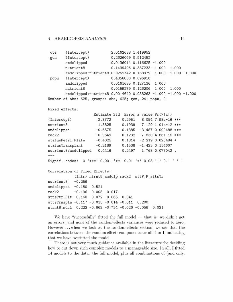
> summary(mp_fits$full)
Generalized linear mixed model fit by the Laplace approximation
Formula: total.fruits ~ nutrient * amd + rack + status + (amd * nutrient | popu) + (amd * nutrient | gen) + (1 | obs)
Data: dat.tf
AIC BIC logLik deviance
2682 2806 -1313 2626
Random effects:
Groups Name Variance Std.Dev. Corr
4 ARABIDOPSIS ANALYSIS 14
obs (Intercept) 2.0162638 1.419952
gen (Intercept) 0.2626069 0.512452
amdclipped 0.0136014 0.116625 -1.000
nutrient8 0.1499496 0.387233 -1.000 1.000
amdclipped:nutrient8 0.0252742 0.158979 1.000 -1.000 -1.000
popu (Intercept) 0.4856830 0.696910
amdclipped 0.0161635 0.127136 1.000
nutrient8 0.0159279 0.126206 1.000 1.000
amdclipped:nutrient8 0.0014640 0.038263 -1.000 -1.000 -1.000
Number of obs: 625, groups: obs, 625; gen, 24; popu, 9
Fixed effects:
Estimate Std. Error z value Pr(>|z|)
(Intercept) 2.3772 0.2951 8.054 7.98e-16 ***
nutrient8 1.3825 0.1939 7.129 1.01e-12 ***
amdclipped -0.6575 0.1885 -3.487 0.000488 ***
rack2 -0.9649 0.1232 -7.830 4.86e-15 ***
statusPetri.Plate -0.4025 0.1814 -2.219 0.026484 *
statusTransplant -0.2189 0.1538 -1.423 0.154607
nutrient8:amdclipped 0.4416 0.2497 1.768 0.077042 .
---
Signif. codes: 0 ‘***’ 0.001 ‘**’ 0.01 ‘*’ 0.05 ‘.’ 0.1 ‘ ’ 1
Correlation of Fixed Effects:
(Intr) ntrnt8 amdclp rack2 sttP.P sttsTr
nutrient8 -0.256
amdclipped -0.150 0.521
rack2 -0.196 0.005 0.017
sttsPtr.Plt -0.160 0.072 0.065 0.041
sttsTrnspln -0.117 -0.015 -0.014 -0.011 0.200
ntrnt8:mdcl 0.222 -0.662 -0.734 -0.026 -0.058 0.021
We have “successfully” fitted the full model — that is, we didn’t getan errors, and none of the random-effects variances were reduced to zero.However . . . when we look at the random-effects section, we see that thecorrelations between the random effects components are all -1 or 1, indicatingthat we have overfitted the model.
There is not very much guidance available in the literature for decidinghow to cut down such complex models to a manageable size. In all, I fitted14 models to the data: the full model, plus all combinations of (amd only,
4 ARABIDOPSIS ANALYSIS 15
nutrient only, intercept only) varying at the population or genotype level (9models), plus a model with only an intercept effect of genotype or population(no random effects at the other level), or an observation-level random effectonly (no effects of population or genotype).
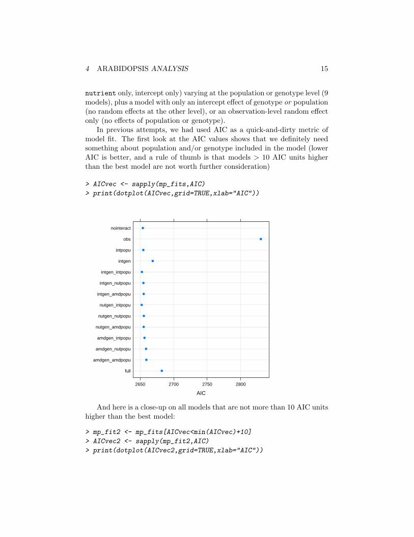
In previous attempts, we had used AIC as a quick-and-dirty metric ofmodel fit. The first look at the AIC values shows that we definitely needsomething about population and/or genotype included in the model (lowerAIC is better, and a rule of thumb is that models > 10 AIC units higherthan the best model are not worth further consideration)
> AICvec <- sapply(mp_fits,AIC)
> print(dotplot(AICvec,grid=TRUE,xlab="AIC"))
AIC
full
amdgen_amdpopu
amdgen_nutpopu
amdgen_intpopu
nutgen_amdpopu
nutgen_nutpopu
nutgen_intpopu
intgen_amdpopu
intgen_nutpopu
intgen_intpopu
intgen
intpopu
obs
nointeract
2650 2700 2750 2800
●
●
●
●
●
●
●
●
●
●
●
●
●
●
And here is a close-up on all models that are not more than 10 AIC unitshigher than the best model:
> mp_fit2 <- mp_fits[AICvec<min(AICvec)+10]
> AICvec2 <- sapply(mp_fit2,AIC)
> print(dotplot(AICvec2,grid=TRUE,xlab="AIC"))
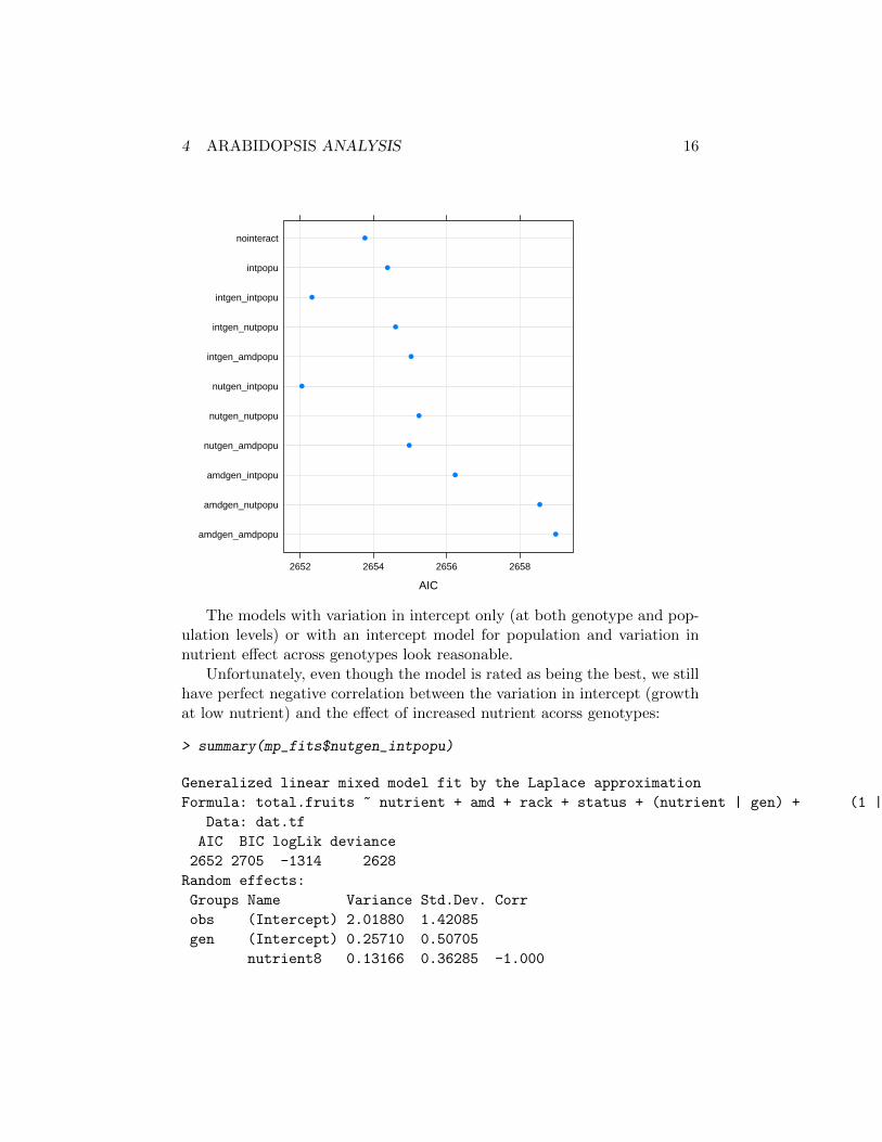
4 ARABIDOPSIS ANALYSIS 16
AIC
amdgen_amdpopu
amdgen_nutpopu
amdgen_intpopu
nutgen_amdpopu
nutgen_nutpopu
nutgen_intpopu
intgen_amdpopu
intgen_nutpopu
intgen_intpopu
intpopu
nointeract
2652 2654 2656 2658
●
●
●
●
●
●
●
●
●
●
●
The models with variation in intercept only (at both genotype and pop-ulation levels) or with an intercept model for population and variation innutrient effect across genotypes look reasonable.
Unfortunately, even though the model is rated as being the best, we stillhave perfect negative correlation between the variation in intercept (growthat low nutrient) and the effect of increased nutrient acorss genotypes:
> summary(mp_fits$nutgen_intpopu)
Generalized linear mixed model fit by the Laplace approximation
Formula: total.fruits ~ nutrient + amd + rack + status + (nutrient | gen) + (1 | popu) + (1 | obs) + nutrient:amd
Data: dat.tf
AIC BIC logLik deviance
2652 2705 -1314 2628
Random effects:
Groups Name Variance Std.Dev. Corr
obs (Intercept) 2.01880 1.42085
gen (Intercept) 0.25710 0.50705
nutrient8 0.13166 0.36285 -1.000

4 ARABIDOPSIS ANALYSIS 17
popu (Intercept) 0.71573 0.84601
Number of obs: 625, groups: obs, 625; gen, 24; popu, 9
Fixed effects:
Estimate Std. Error z value Pr(>|z|)
(Intercept) 2.3802 0.3354 7.096 1.29e-12 ***
nutrient8 1.3793 0.1870 7.375 1.64e-13 ***
amdclipped -0.6707 0.1822 -3.682 0.000232 ***
rack2 -0.9615 0.1233 -7.797 6.33e-15 ***
statusPetri.Plate -0.3994 0.1817 -2.198 0.027916 *
statusTransplant -0.2209 0.1539 -1.435 0.151327
nutrient8:amdclipped 0.4449 0.2473 1.799 0.071992 .
---
Signif. codes: 0 ‘***’ 0.001 ‘**’ 0.01 ‘*’ 0.05 ‘.’ 0.1 ‘ ’ 1
Correlation of Fixed Effects:
(Intr) ntrnt8 amdclp rack2 sttP.P sttsTr
nutrient8 -0.379
amdclipped -0.254 0.445
rack2 -0.172 0.004 0.018
sttsPtr.Plt -0.141 0.074 0.066 0.041
sttsTrnspln -0.101 -0.018 -0.015 -0.011 0.199
ntrnt8:mdcl 0.189 -0.621 -0.738 -0.027 -0.057 0.020
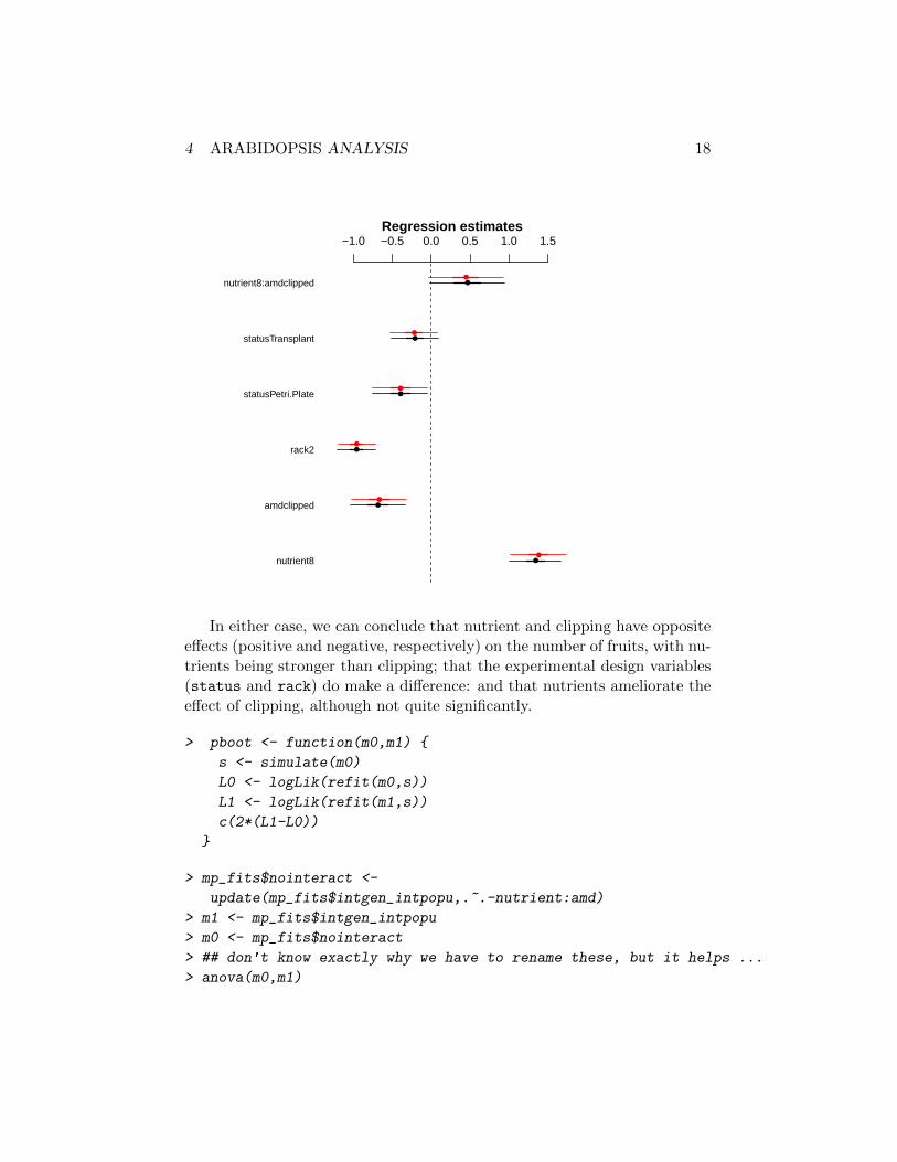
For what it’s worth, including or excluding the random effect of nutrientat the genotype level has very little effect on the estimates of the fixed effects:
> source("coefplot_new.R")
> coefplot(list(mp_fits$intgen_intpopu,mp_fits$nutgen_intpopu),intercept=FALSE)
4 ARABIDOPSIS ANALYSIS 18
Regression estimates−1.0 −0.5 0.0 0.5 1.0 1.5
nutrient8
amdclipped
rack2
statusPetri.Plate
statusTransplant
nutrient8:amdclipped
●
●
●
●
●
●
●
●
●
●
●
●
In either case, we can conclude that nutrient and clipping have oppositeeffects (positive and negative, respectively) on the number of fruits, with nu-trients being stronger than clipping; that the experimental design variables(status and rack) do make a difference: and that nutrients ameliorate theeffect of clipping, although not quite significantly.
> pboot <- function(m0,m1) {
s <- simulate(m0)
L0 <- logLik(refit(m0,s))
L1 <- logLik(refit(m1,s))
c(2*(L1-L0))
}
> mp_fits$nointeract <-
update(mp_fits$intgen_intpopu,.~.-nutrient:amd)
> m1 <- mp_fits$intgen_intpopu
> m0 <- mp_fits$nointeract
> ## don't know exactly why we have to rename these, but it helps ...
> anova(m0,m1)

4 ARABIDOPSIS ANALYSIS 19
Data: dat.tf
Models:
m0: total.fruits ~ nutrient + amd + rack + status + (1 | gen) + (1 |
m0: popu) + (1 | obs)
m1: total.fruits ~ nutrient + amd + rack + status + (1 | gen) + (1 |
m1: popu) + (1 | obs) + nutrient:amd
Df AIC BIC logLik Chisq Chi Df Pr(>Chisq)
m0 9 2653.8 2693.7 -1317.9
m1 10 2652.3 2696.7 -1316.2 3.4465 1 0.06339 .
---
Signif. codes: 0 ‘***’ 0.001 ‘**’ 0.01 ‘*’ 0.05 ‘.’ 0.1 ‘ ’ 1
The parametric bootstrap takes about 12 seconds per replicate, so youshouldn’t try to run the following code — the results are read in from thebatch file.
(Don’t actually do this unless you want to spend a long time!)
> pbootdist <- replicate(1000,pboot(mp_fits$nointeract,mp_fits$intgen_intpopu))
> obsdev <- (2*(logLik(m1)-logLik(m0)))
> (pval.nominal <- c(pchisq(obsdev,df=1,lower.tail=FALSE)))
[1] 0.06338761
> (pval.PB <- mean(pbootdist>obsdev))
[1] 0.073
> hist(pbootdist,freq=FALSE,breaks=100,col="gray")
> lines(density(pbootdist,from=0),col=2)
> curve(dchisq(x,df=1),col=4,add=TRUE)
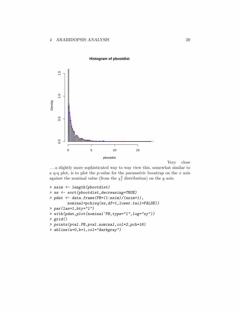
4 ARABIDOPSIS ANALYSIS 20
Histogram of pbootdist
pbootdist
Den
sity
0 5 10 15
0.0
0.5
1.0
1.5
Very close. . . a slightly more sophisticated way to way view this, somewhat similar toa q-q plot, is to plot the p-value for the parametric boostrap on the x axisagainst the nominal value (from the χ2
1 distribution) on the y axis.
> nsim <- length(pbootdist)
> ss <- sort(pbootdist,decreasing=TRUE)
> pdat <- data.frame(PB=(1:nsim)/(nsim+1),
nominal=pchisq(ss,df=1,lower.tail=FALSE))
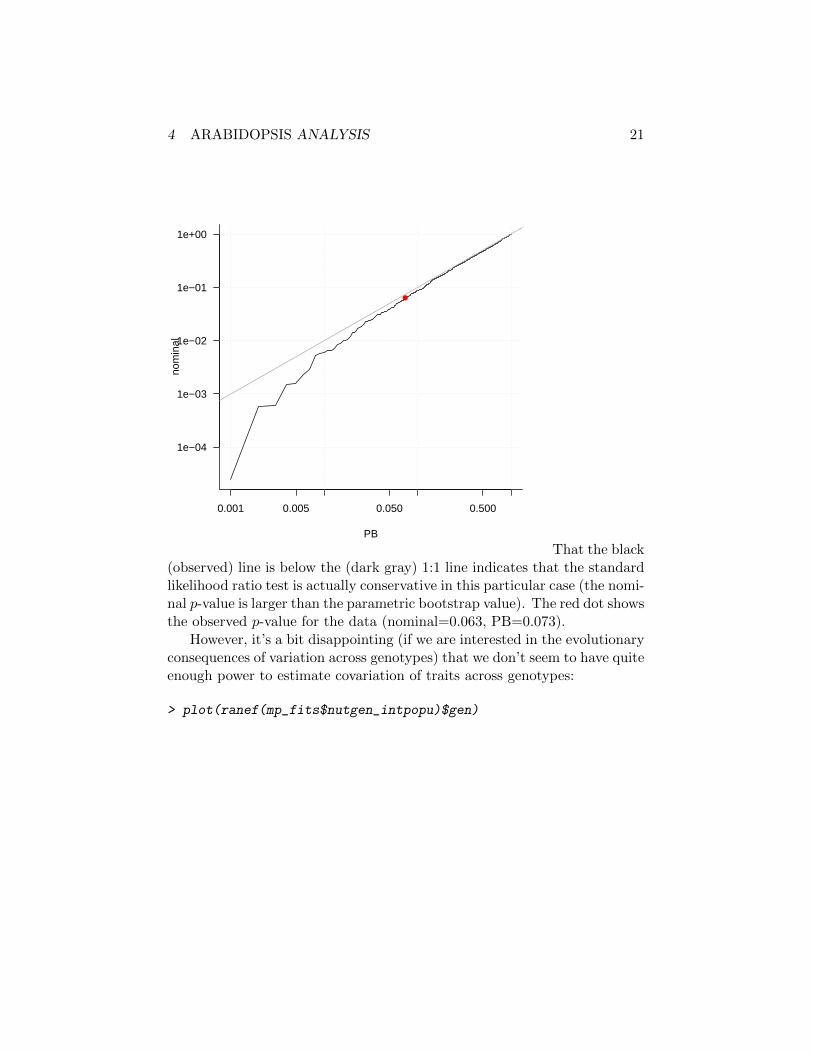
> par(las=1,bty="l")
> with(pdat,plot(nominal~PB,type="l",log="xy"))
> grid()
> points(pval.PB,pval.nominal,col=2,pch=16)
> abline(a=0,b=1,col="darkgray")
4 ARABIDOPSIS ANALYSIS 21
0.001 0.005 0.050 0.500
1e−04
1e−03
1e−02
1e−01
1e+00
PB
nom
inal
●
That the black(observed) line is below the (dark gray) 1:1 line indicates that the standardlikelihood ratio test is actually conservative in this particular case (the nomi-nal p-value is larger than the parametric bootstrap value). The red dot showsthe observed p-value for the data (nominal=0.063, PB=0.073).
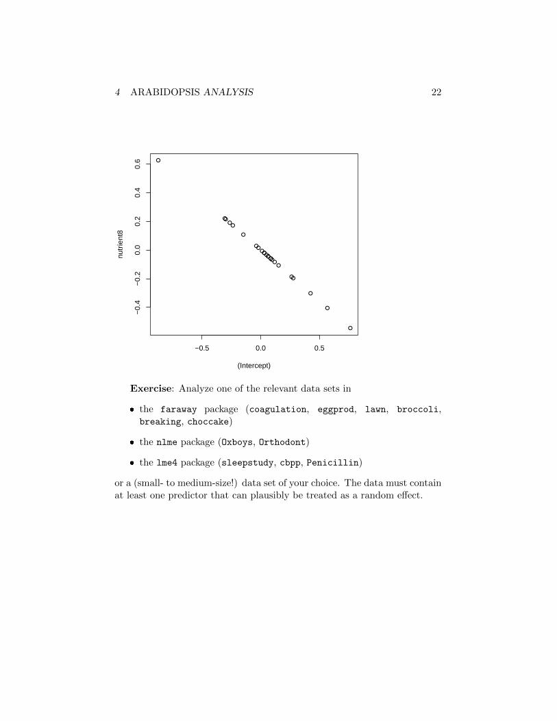
However, it’s a bit disappointing (if we are interested in the evolutionaryconsequences of variation across genotypes) that we don’t seem to have quiteenough power to estimate covariation of traits across genotypes:
> plot(ranef(mp_fits$nutgen_intpopu)$gen)
4 ARABIDOPSIS ANALYSIS 22
●
●
●●
●
●●●
●
●●
●
●
●
●
●
●
●
●
●
●
●
●
●
−0.5 0.0 0.5
−0.
4−
0.2
0.0
0.2
0.4
0.6
(Intercept)
nutr
ient
8
Exercise: Analyze one of the relevant data sets in
� the faraway package (coagulation, eggprod, lawn, broccoli,breaking, choccake)
� the nlme package (Oxboys, Orthodont)
� the lme4 package (sleepstudy, cbpp, Penicillin)
or a (small- to medium-size!) data set of your choice. The data must containat least one predictor that can plausibly be treated as a random effect.