LITERATURE REVIEW IN SUPPORT OF PAMS PROGRAM ASSESSMENT › projects › regional-pams-assessment › nescaum … · LITERATURE REVIEW IN SUPPORT OF PAMS PROGRAM ASSESSMENT FINAL

LITERATURE REVIEW IN SUPPORT OFPAMS PROGRAM ASSESSMENT

FINAL REPORTSTI-900860-2039-FR

By:Charles L. Blanchard

ENVAIR526 Cornell AvenueAlbany, CA 94706

Hilary H. MainSonoma Technology, Inc.

1360 Redwood Way, Suite CPetaluma, CA 94954-1169

Prepared for:Gary Kleiman

NESCAUM129 Portland Street, Suite 501

Boston, MA 02114

June 1, 2001

1360 Redwood Way, Suite CPetaluma, CA 94954-1169

707/665-9900FAX 707/665-9800

www.sonomatech.com

This page is intentionally blank.

iii

PREFACE

This report summarizes a literature review performed as Task 1 of a project for theNortheast States for Coordinated Air Use Management (NESCAUM) and the Mid-AtlanticRegional Air Management Association (MARAMA) to aid in analyzing and interpretingPhotochemical Assessment Monitoring Station (PAMS) data and in recommendingimprovements to PAMS operations. In this task, we reviewed PAMS-related scientific literature,government reports, and previous literature reviews pertaining to analysis of PAMS andPAMS-like data in the NESCAUM and MARAMA regions, in other regions, and in otherresearch and field studies. The report includes summaries of selected key analysis report,recommendations concerning specific data management or analysis techniques that could beapplied to PAMS data, and a bibliography.

The goal of this task is to investigate how PAMS (and similar) data have been—or couldbe—used to meet PAMS objectives, with special emphasis on evaluating potential modificationsto the existing network.

This literature review was used in later tasks of the project to help us formulaterecommendations concerning monitoring, data management, and data analysis methods thatcould be applied to PAMS data to meet the PAMS program objectives.

Please refer to Main and Roberts (2001) for final recommendations to the Northeast andMid-Atlantic States PAMS program.

Main H.H. and Roberts P.T. (2001) Recommendations for the PAMS network in theNortheast and Mid-Atlantic states. Final report prepared for NESCAUM, Boston, MA,by Sonoma Technology, Inc., Petaluma, CA, STI-900860-2067-FR, June. Also availableat <http://www.nescaum.org/committees/pams.html>.

This page is intentionally blank.

v

TABLE OF CONTENTS

Section Page

PREFACE ...................................................................................................................................... iiiLIST OF FIGURES.......................................................................................................................viiLIST OF TABLES ........................................................................................................................vii

1. INTRODUCTION ..............................................................................................................1-11.1 Task Objectives ........................................................................................................1-11.2 PAMS Program Background ....................................................................................1-1

1.2.1 Monitoring Information ................................................................................1-11.2.2 Pams Data Analysis Objectives ....................................................................1-2

1.3 Approach...................................................................................................................1-41.4 Review of Literature and Evaluation of Objectives..................................................1-4

1.4.1 Track Progress ..............................................................................................1-51.4.2 Improve Emission Inventories ......................................................................1-51.4.3 Identify Key Constituents and Parameters....................................................1-51.4.4 Characterize Transport..................................................................................1-51.4.5 Apply and Evaluate Photochemical Models.................................................1-5

2. SUMMARY OF LITERATURE REVIEW .......................................................................2-12.1 Tracking Trends........................................................................................................2-1

2.1.1 Applicable Data Analysis Methods ..............................................................2-12.1.2 Limitations of the Methods...........................................................................2-22.1.3 Adequacy of PAMS Data to Support Methods.............................................2-22.1.4 Recommendations.........................................................................................2-3

2.2 Improving Emission Inventories...............................................................................2-42.2.1 Applicable Data Analysis Methods ..............................................................2-42.2.2 Limitations of the Methods...........................................................................2-52.2.3 Adequacy of PAMS Data to Support Methods.............................................2-62.2.4 Recommendations.........................................................................................2-7

2.3 Identifying Key Constituents And Parameters Involved In PhotochemicalOzone Formation ......................................................................................................2-82.3.1 Applicable Data Analysis Methods ..............................................................2-82.3.2 Limitations of the Methods...........................................................................2-92.3.3 Adequacy of PAMS Data to Support Methods...........................................2-102.3.4 Recommendations.......................................................................................2-11

2.4 Characterizing Transport ........................................................................................2-142.4.1 Applicable Data Analysis Methods ............................................................2-142.4.2 Limitations of the Methods.........................................................................2-182.4.3 Adequacy of PAMS Data to Support Methods...........................................2-182.4.4 Recommendations.......................................................................................2-18

vi

TABLE OF CONTENTS (Concluded)

Section Page

2.5 Providing Data For Model Application And Evaluation ........................................2-192.5.1 Applicable Data Analysis Methods ............................................................2-192.5.2 Limitations of the Methods.........................................................................2-202.5.3 Adequacy of PAMS Data to Support Methods...........................................2-202.5.4 Recommendations.......................................................................................2-22

2.6 Forecasting Episodes ..............................................................................................2-222.6.1 Applicable Data Analysis Methods ............................................................2-222.6.2 Recommendations.......................................................................................2-22

2.7 Other Uses of PAMS Data......................................................................................2-22

3. RECOMMENDATIONS....................................................................................................3-13.1 General Recommendations for the PAMS Network.................................................3-1

3.1.1 Number of Sites of Each Type......................................................................3-13.1.2 Species Measured at Each Site .....................................................................3-13.1.3 Frequency and Resolution of Measurements................................................3-2

3.2 Specific Recommendations for the NESCAUM and MARAMA Regions—Preliminary and Contingent Upon Completion of Data Analyses............................3-23.2.1 Number of Sites of Each Type......................................................................3-33.2.2 Species, Frequency, and Resolution of Measurements at Each Site ............3-3

4. REFERENCES ...................................................................................................................4-1

APPENDIX A: BIBLIOGRAPHY ...........................................................................................A-1

vii

LIST OF FIGURES

Figure Page

2-1. Summary statistics describing an indicator of VOC or NOx limitation during the1995 NARSTO-Northeast study......................................................................................2-12

2-2. Aloft ozone concentrations on the morning of June 19, 1995, at three locations............2-16

2-3. Aloft ozone concentrations on the morning of July 14, 1995, at three locations ............2-17

LIST OF TABLES

Table Page

1-1. Decision matrix to be used to identify example activities that will help the analystaddress scientific/technical questions and objectives ........................................................1-5

2-1. Site key for Figure 2-1.....................................................................................................2-13

2-2. EPA ORD priorities for use of PAMS data for model evaluation...................................2-21

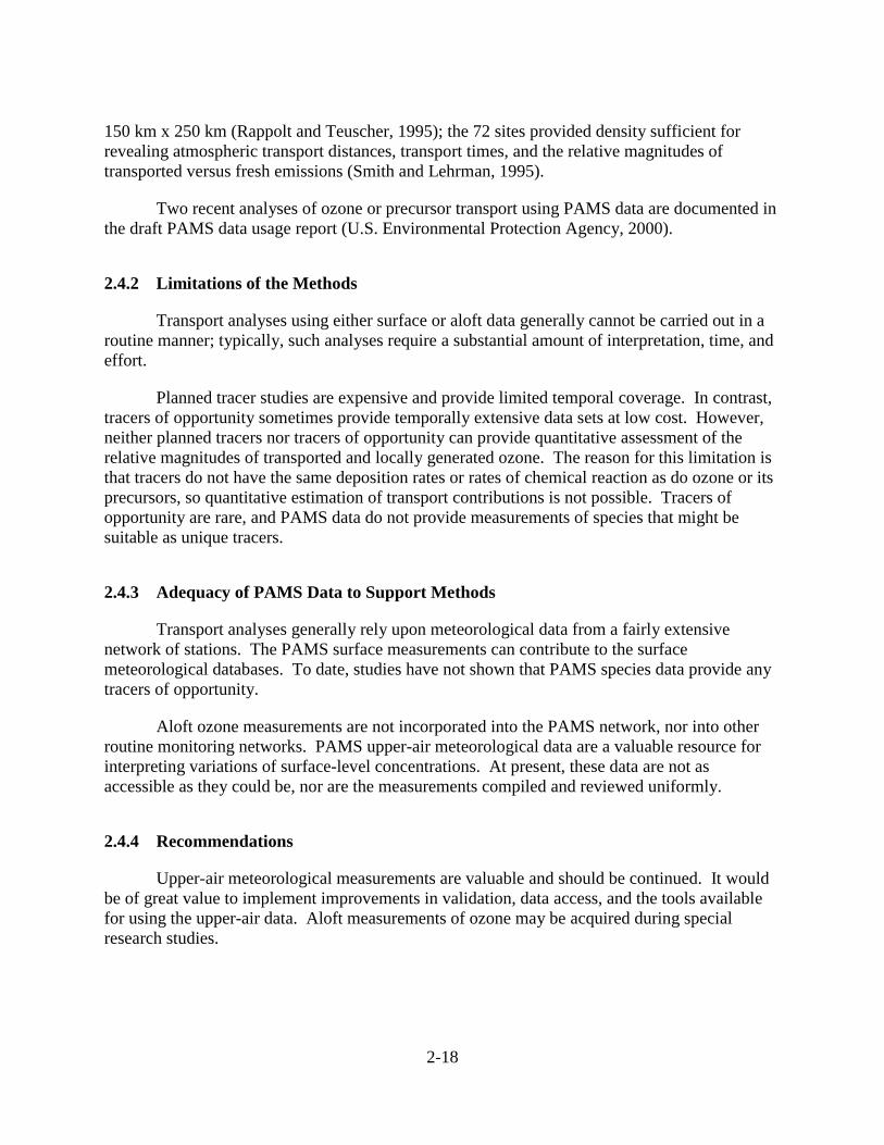
3-1. PAMS monitoring sites in the NESCAUM and MARAMA regions ................................3-5

1-1

1. INTRODUCTION

This report summarizes a literature review performed as Task 1 of a project for theNortheast States for Coordinated Air Use Management (NESCAUM) and the Mid-AtlanticRegional Air Management Association (MARAMA) to aid in analyzing and interpretingPhotochemical Assessment Monitoring Station (PAMS) data and in recommendingimprovements to PAMS operations.

1.1 TASK OBJECTIVES

The goal of this task is to investigate how PAMS (and similar) data have been – or couldbe – used to meet PAMS objectives, with special emphasis on evaluating potentialmodifications to the existing network. We reviewed scientific literature, government reports,and previous literature reviews pertaining to analysis of PAMS and PAMS-like data in theNESCAUM and MARAMA regions, in other regions, and in other research and field studies.We provide a review of selected key analysis reports, recommendations concerning specific datamanagement or analysis techniques that could be applied to PAMS data in the NESCAUM andMARAMA regions, and a bibliography.

1.2 PAMS PROGRAM BACKGROUND

1.2.1 Monitoring Information

State and local air pollution control agencies operate the PAMS sites. The PAMSnetworks typically monitor 56 target hydrocarbons and 2 carbonyl compounds, ozone, oxides ofnitrogen (NOx and/or NOy), and meteorological measurements. Sample speciation may varyamong sites as some agencies report more hydrocarbons and/or carbonyl compounds than thePAMS target list. Differences among analytical techniques also can alter the list (e.g.,co-eluters).

The sampling frequency varies among regions, states, and sites in the PAMS program.For example, hydrocarbons are sampled on a 1-hr or 3-hr average basis; may or may not cover a24-hr period; and are collected every day, every third day, or on an episodic basis. Carbonylcompounds are typically collected as 3-hr averages every third day but other sampling variationsexist. Most sites take surface meteorological measurements, including wind speed, winddirection, and temperature reported hourly. PAMS program upper-air meteorologicalmeasurement requirements may be met in a number of ways, including using rawinsondes, radarprofilers, or twice daily National Weather Service soundings.

The number of PAMS sites varies among metropolitan statistical areas (MSAs). Ozoneprecursors (volatile organic compounds [VOC] and NOx) and surface meteorology are requiredto be measured at two to five sites in an MSA, depending on the MSA population. Upper-airmeteorology must be monitored at one representative site in an MSA. PAMS measurements

1-2

(U.S. Environmental Protection Agency, 2001) are made at different site types that have differentmeasurement objectives:

• Type 1 – Upwind and background characterization site.

• Type 2 and 2A – Maximum ozone precursor emissions impact site.

• Type 3 – Maximum ozone concentration site.

• Type 4 – Extreme downwind monitoring site.

It is convenient to use the site types as defined by the EPA to discuss the PAMS data inthis report because the PAMS monitoring and analysis community is familiar with thedesignations. In a geographic region such as the Northeast and Mid-Atlantic, the site types maybe clearly defined from a political boundary point of view but may be less clearly defined in theregion as a whole. For example, a Type 4 site may also be a Type 1 site for another MSA. Forthis project, the data from each site were analyzed with respect to the proximity of the site tosources, age of air mass, diurnal characteristics, etc. rather than solely relying on site type.

1.2.2 PAMS DATA ANALYSIS OBJECTIVES

Analyses of PAMS data were originally intended to fulfill eleven objectives:

National Ambient Air Quality Standard (NAAQS) Attainment and Control StrategyDevelopment

1. Attainment/nonattainment determinations2. Assessment of the relative contributions of local and upwind sources3. Boundary conditions for photochemical modeling4. Episode selection5. Model evaluation

State Implementation Plan (SIP) Control Strategy Evaluation

6. Evaluation of the effectiveness of implemented control strategies

Emissions Tracking

7. Corroboration of nitrogen oxides (NOx) and volatile organic compound (VOC)inventories and trends

8. Corroboration of VOC species source profiles

9. Analysis of air toxics

Ambient Trend Appraisals

10. Trends for ozone (O3), NOx, total and speciated VOC, including adjustments forvariations in meteorological conditions

Exposure Assessment

11. Estimation of risk levels and the size of affected populations

1-3

A set of refocused objectives was developed in a recent State and Territorial Air PollutionProgram Administrators/Association of Local Air Pollution Control Officials(STAPPA/ALAPCO) PAMS workshop (STAPPA/ALAPCO, 2000). We have structured ourreview according to the refocused objectives. For convenience, we have mapped the originalgoals to the refocused objectives. The numbers in brackets below identify the original PAMSobjectives, mapping each to one or more of the newer objectives. In addition, we have addedone objective [see (v) below] that more explicitly includes the original PAMS objectivespertaining to photochemical model development and evaluation. The refocused objectives are to

Help assess ozone control programs by

(i) tracking trends [10],

(ii) assisting in improving emission inventories [7, 8],

(iii) identifying key constituents and parameters involved in photochemical ozone formation[6],

(iv) characterizing transport [2],

(v) providing data for model application and evaluation [3, 4, 5], and

(vi) assisting in forecasting episodes [new].

Use PAMS data to benefit other programs by

(vii) helping to characterize ambient air toxics for exposure modeling and trend analyses[9, 11],

(viii) helping to characterize emissions and ambient concentrations of nitrogen species[7, 10],

(ix) providing data for evaluation of particulate matter [new], and

(x) enhancing special studies [3, 4, 5].

Our review focuses on the first six objectives (i-vi) – those pertaining to the use of PAMSdata for evaluating the effectiveness of ozone control programs. Although these six primaryobjectives are of broad interest, in the context of the PAMS program we consider themprincipally in relation to the ongoing assessment of control strategies. For example, trendassessment is a key PAMS data-analysis objective because it is the principal means fordocumenting rates of progress toward attainment of the federal 1-hr or proposed 8-hr ozonestandards. Similarly, accurate emission inventories are needed to focus control efforts on themost important sources; the PAMS data can be used to improve emission inventories. Inaddition, our understanding of the atmospheric processes involved in photochemical ozoneformation, while of general scientific interest, is of specific regulatory interest as to how itaffects decisions about sources to control and the levels of emissions control required.

1-4

1.3 APPROACH

We first defined PAMS data analysis objectives (Section 1.1.2). For each objective, we1. describe applicable data analysis methods,2. give example applications,3. discuss limitations of the methodologies,4. discuss limitations of the data (focusing on the capability of the data for supporting

methodologies), and5. provide recommendations for PAMS.

1.4 REVIEW OF LITERATURE AND EVALUATION OF OBJECTIVES

The types of data and data analyses needed to support the six primary, refocused PAMSanalysis objectives are identified in summary form in Table 1. This table lists the six primaryPAMS data analysis objectives and identifies specific technical questions associated with eachobjective. For each technical question, the table identifies one or more data analysis approaches(indicated as “x”s in the row for each question). By following the column for each approach tothe second page, the table identifies specific measurements, techniques, or computer software(indicated as “x”s in the column for each data analysis approach). These approaches andtechniques are discussed in detail in the following sections. A recent draft report (U.S.Environmental Protection Agency, 2000) documents 38 studies that have recently beencompleted using PAMS data. One or more of each of eleven types of analyses described in thePAMS workbook was conducted in the set of 38 studies. Some of those studies are included asexamples in later sections of this report.

1-5

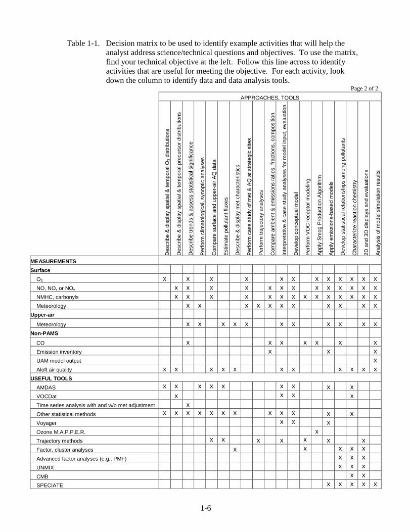
Table 1-1. Decision matrix to be used to identify example activities that will help theanalyst address scientific/technical questions and objectives. To use thematrix, find your technical objective at the left. Follow this line across toidentify activities that are useful for meeting the objective. For each activity,look down the column to identify data and data analysis tools.

Page 1 of 2APPROACHES, TOOLS

Des

crib

e &

disp

lay

spat

ial &

tem

pora

l O3 d

istri

butio

ns

Des

crib

e &

disp

lay

spat

ial &

tem

pora

l pre

curs

or d

istri

butio

ns

Des

crib

e tre

nds

& as

sess

sta

tistic

al s

igni

fican

ce

Perfo

rm c

limat

olog

ical

, syn

optic

ana

lyse

s

Com

pare

sur

face

and

upp

er-a

ir AQ

dat

a

Estim

ate

pollu

tant

flux

es

Des

crib

e &

disp

lay

met

cha

ract

eris

tics

Perfo

rm c

ase

stud

y of

met

& A

Q a

t stra

tegi

c si

tes

Perfo

rm tr

ajec

tory

ana

lyse

s

Com

pare

am

bien

t & e

mis

sion

s ra

tios,

frac

tions

, com

posi

tion

Inte

rpre

tativ

e &

case

stu

dy a

naly

ses

for m

odel

inpu

t, ev

alua

tion

Dev

elop

con

cept

ual m

odel

Perfo

rm V

OC

rece

ptor

mod

elin

g

Appl

y Sm

og P

rodu

ctio

n Al

gorit

hm

Appl

y em

issi

ons-

base

d m

odel

s

Dev

elop

sta

tistic

al re

latio

nshi

ps a

mon

g po

lluta

nts

Cha

ract

eriz

e re

actio

n ch

emis

try

2D a

nd 3

D d

ispl

ays

and

eval

uatio

ns

Anal

ysis

of m

odel

sim

ulat

ion

resu

lts

SCIENCE/TECHNICAL QUESTIONS/OBJECTIVES

Assess ozone trends xAssess precursor trends x

Evaluate emissions inventories x x xPerform source attribution x x x

Assess O3 concentration distributions x xCharacterize precursor concentration distributions x xCharacterize meteorological processes x x xDescribe climatological patterns xAscertain VOC sources (natural vs. anthropogenic) x xAssess VOC and/or NOx reduction influence on O3 x x x x x

Estimate fluxes into and within region x x xAssess contribution of subregions, carryover x x

Obtain data for model initial, boundary conditions xEvaluate air quality models x x x x xEvaluate meteorological models x x x xDetermine met & AQ phenomena to be reproduced x x x x

Forecast episodesAssess precursors with respect to O3concentrations x x x x x

1-6

Table 1-1. Decision matrix to be used to identify example activities that will help theanalyst address science/technical questions and objectives. To use the matrix,find your technical objective at the left. Follow this line across to identifyactivities that are useful for meeting the objective. For each activity, lookdown the column to identify data and data analysis tools.

Page 2 of 2APPROACHES, TOOLS

Des

crib

e &

disp

lay

spat

ial &

tem

pora

l O3 d

istri

butio

ns

Des

crib

e &

disp

lay

spat

ial &

tem

pora

l pre

curs

or d

istri

butio

ns

Des

crib

e tre

nds

& as

sess

sta

tistic

al s

igni

fican

ce

Perfo

rm c

limat

olog

ical

, syn

optic

ana

lyse

s

Com

pare

sur

face

and

upp

er-a

ir AQ

dat

a

Estim

ate

pollu

tant

flux

es

Des

crib

e &

disp

lay

met

cha

ract

eris

tics

Perfo

rm c

ase

stud

y of

met

& A

Q a

t stra

tegi

c si

tes

Perfo

rm tr

ajec

tory

ana

lyse

s

Com

pare

am

bien

t & e

mis

sion

s ra

tios,

frac

tions

, com

posi

tion

Inte

rpre

tativ

e &

case

stu

dy a

naly

ses

for m

odel

inpu

t, ev

alua

tion

Dev

elop

con

cept

ual m

odel

Perfo

rm V

OC

rece

ptor

mod

elin

g

Appl

y Sm

og P

rodu

ctio

n Al

gorit

hm

Appl

y em

issi

ons-

base

d m

odel

s

Dev

elop

sta

tistic

al re

latio

nshi

ps a

mon

g po

lluta

nts

Cha

ract

eriz

e re

actio

n ch

emis

try

2D a

nd 3

D d

ispl

ays

and

eval

uatio

ns

Anal

ysis

of m

odel

sim

ulat

ion

resu

lts

MEASUREMENTSSurface

O3 x x x x x x x x x x x xNO, NOx or NOy x x x x x x x x x x x x xNMHC, carbonyls x x x x x x x x x x x x x xMeteorology x x x x x x x x x x x

Upper-air Meteorology x x x x x x x x x x x

Non-PAMS CO x x x x x x xEmission inventory x x xUAM model output xAloft air quality x x x x x x x x x x x

USEFUL TOOLS AMDAS x x x x x x x x xVOCDat x x x xTime series analysis with and w/o met adjustment xOther statistical methods x x x x x x x x x x x xVoyager x x xOzone M.A.P.P.E.R. xTrajectory methods x x x x x x xFactor, cluster analyses x x x x xAdvanced factor analyses (e.g., PMF) x x xUNMIX x x xCMB x xSPECIATE x x x x x

2-1

2. SUMMARY OF LITERATURE REVIEW

2.1 TRACKING TRENDS

2.1.1 Applicable Data Analysis Methods

Rates of progress toward attainment of the ozone standard are tracked by analyzingtrends in ozone concentrations. Indeed, quantifying rates of progress is a necessary part of theSIP process. However, understanding the factors that are responsible for the observed trendsrequires additional analyses, including characterizations of trends in precursor concentrations.Moreover, because ozone formation is highly nonlinear, examining trends in precursorconcentrations is the most direct way to investigate the effects of emission control programs.Trends in precursor concentrations may be used to corroborate changes in emission inventories.

While many statistical techniques have been employed to detect air pollutant trends, theymay be conveniently categorized using the following dichotomies:

• Analysis of hourly concentration data versus seasonal or monthly statistics, such as theannual maximum hourly concentration.

• Analysis of statistics closely related to the ozone standard versus more robust air-qualityindicators. For example, the fourth-highest hourly ozone maximum during eachthree-year period is closely linked with the expected-exceedance form of the federal1-hr ozone standard, but is known to exhibit considerable year-to-year variability. Toimprove the signal-to-noise ratio, the California Air Resources Board (ARB) includesanalyses of trends in the average of the top 30 daily ozone 1-hr maxima each year.

• Incorporation versus no incorporation of adjustments for year-to-year variations inmeteorological phenomena that influence the rate of ozone formation.

Because ozone concentrations are highly correlated from hour to hour and even from day to day,analyses based upon hourly or daily data must be carried out using reasonably sophisticatedstatistical time series techniques. Besides accounting for the correlation structure within thedata, such techniques also incorporate filtering (Rao and Zurbenko, 1994; Rao et al., 1999) orsmoothing (Sirois, 1993) procedures for extracting linear, nonlinear, or step changes that aretypically small in relation to the wide variations observed in the hourly or daily ozoneconcentrations. Simpler regression techniques are appropriate for annual statistics. Usually,either substantial averaging of the data (e.g., the top 30 ozone maxima) or adjustment formeteorological variations that influence the annual extreme concentrations (e.g., fourth-highesthourly maximum during each three-year period) is needed to obtain detectable trends overperiods of less than ten years.

Twelve recent analyses of ozone or precursor trends using PAMS data are documented inthe draft PAMS data usage report (U.S. Environmental Protection Agency, 2000).

2-2

2.1.2 Limitations of the Methods

Trends in ozone and other species of interest are difficult to quantify because the majorityof the day-to-day, and even year-to-year, variation in concentrations is attributable to variationsin weather. This variation cannot be removed by simply adding more monitoring locationsbecause all locations within a particular area experience the same weather patterns and tend toshow highly correlated variations in concentrations.

Because ozone is a secondary pollutant, concentration variations are affected by changesin the concentrations of many other chemical species. Therefore, documenting the effects of anemission rule is more readily accomplished by examining trends in specific primary pollutants,rather than in ozone.

The utility of trend analyses depends upon the magnitudes of emission reductions, thequality and length of record of the monitoring data, and the relative magnitudes of the emissions-and weather-driven variations in ambient pollutant concentrations (Blanchard, 2000). For asignal-to-noise ratio of 1:1, about two to four years of monthly data are needed to detect a lineartrend with high probability (90%) at a 95% confidence level, whereas 10 to 20 years of data areneeded when the signal-to-noise ratio falls to 0.1:1 (Weatherhead et al., 1998). Variations inurban ozone concentrations are dominated by weather; temperature variations, random variation,and emissions-related trends have been shown to account for 70%, 20%, and 10%, respectively,of the total variance of ozone concentrations at several monitoring locations (Rao and Zurbenko,1994; Rao et al., 1999). Given such an unfavorable ratio of signal to noise (~0.1:1), ozone trendanalyses have typically incorporated procedures for adjusting for variations in temperature andother meteorological factors (e.g., Rao and Zurbenko, 1994; Rao et al., 1999; Kolaz andSwinford, 1990; Kuntasal and Chang, 1987; Cassmassi and Bassett, 1993; Zeldin et al., 1991;Stoeckenius, 1991; Cox and Chu, 1993; Shively, 1991; Bloomfield et al., 1996); used statistics(e.g., median, 90th percentile) that are less sensitive to meteorological variations than are theextreme ozone concentrations (Fiore et al., 1998; Korsog and Wolff, 1991; Curran and Frank,1991; Chock et al., 1982); or have averaged data spatially and temporally (Fujita, 1993). Thecapabilities of the methods that have been employed to account for the effects of weathervariations on ozone concentrations have not been systematically compared, so none can beidentified as superior (Rao et al., 1999). Although some success has been achieved in identifyingtrends and demonstrating their qualitative consistency with the magnitudes of emissionreductions, ozone trend analyses generally have not been able to link ambient concentrationswith specific source types or locations. An exception is time series analyses that havedemonstrated step changes in urban ozone concentrations occurring when new emission controlprocedures were implemented, thus quantifying a relationship between the controlled sourcesand ambient ozone concentrations (Milanchus et al., 1998.; Rao and Zurbenko, 1994; Box andTiao, 1975).

2.1.3 Adequacy of PAMS Data to Support Methods

The single most important factor affecting the success of trend analyses is the quality ofthe data record. A long and continuous record is needed, with reasonably complete sampling

2-3

during each ozone season. One site with a high-quality record is more valuable than many siteswith short records or incomplete sampling.

Data are needed to support analyses of trends in ozone and ozone precursorconcentrations. Accurate, high-resolution measurements of NOx (or NOy), carbon monoxide(CO), and total nonmethane hydrocarbons (NMHC) are desirable for this purpose and are notparticularly resource-intensive because they are continuous, hourly measurements. ContinuousCO (ppbv detection limits) and NMHC (50 ppbv detection limits) are not measured at PAMSsites. For tracking total hydrocarbon concentrations, the continuous NMHC measurements (i.e.,not speciated) may be a reasonable, and less resource-demanding, substitute for total nonmethaneorganic compounds (NMOC) (speciated canister samples or gas chromatograph [GC]). Theexception is the need to document changes in specific compounds in relation to the adoption ofnew emission rules. For example, Main et al. (1998; 1999) showed that statistically significantdecreases in ambient benzene weight fractions occurred between 1994 and 1995, coinciding withthe reduction of benzene amounts in the reformulated gasoline that was introduced in 1995. Fortotal NMHC, detection of significant changes is not necessarily expected in a data set of five tosix years; thus, it is important to continue to gather data to compile a longer record.

Spatial representativeness of measurements is an issue for trend analysis when there isreason to suspect that trends differ among locations. For example, urban center trends may differfrom trends in suburban areas due to growth and development, which has largely occurred insuburbs. Nationwide, CO monitors, most of which are in center-city locations, recorded peak8-hr CO concentration declines averaging 39% from 1990 to 1998, a greater than proportionaldecline than the 16% reduction of total CO emissions during the same period (U.S.Environmental Protection Agency, 2000). The data suggest that the CO emission reduction wasmore prominent in the urban centers (i.e., reductions were not offset by growth in vehicle milestraveled near urban-center monitors). It is possible that some areas experiencing high growthrates may have experienced increases in local emission rates. For comparison, peak ozonemonitors are generally located in downwind areas where growth of commute traffic may haveresulted in locally higher ozone precursor loading rates. During the period 1989-98, 104 of139 Metropolitan Statistical Areas (MSAs) exhibited statistically significant declines in thesecond maximum 8-hr CO concentration, whereas only 25 of 198 MSAs showed statisticallysignificant declines in the fourth maximum 8-hr ozone concentration (U.S. EnvironmentalProtection Agency, 2000). (Trends were based upon spatial averages of all monitors within eachMSA.) Ozone concentrations increased at 17 of 24 National Park Service sites where ozone ismonitored (U.S. Environmental Protection Agency, 2000). Anecdotal evidence suggests that atsome sites, declines in peak ozone concentrations appear to be associated with rising NOx levels,and possibly titration of ozone by NO, rather than resulting from reductions of ozone formation.

2.1.4 Recommendations

Trends, and the relationship of ozone to precursor trends, will be best recognized usingcontinuous, complete, and long-term sampling for ozone, CO, NOx (or NOy), and total NMHC(or speciated NMOC) at Type 2 and Type 3 PAMS locations. The principal program needs forPAMS sites are to ensure the continuity of monitoring at existing locations, to addhigh-resolution (ppbv) CO (which will serve other purposes, as discussed in Section 2.2), and to

2-4

replace speciated NMOC with accurate continuous measurements of total NMHC (50 ppbv orbetter resolution) at locations where speciated hydrocarbons might be discontinued for otherreasons (see Section 2.2). Comparability of NMHC to total NMOC measurements should beestablished through a period during which collocated NMHC and NMOC measurements aremade. If trends in carbonyl concentrations are deemed of sufficient interest, an attractive costoption is to replace cartridge sampling with continuous formaldehyde monitors at some Type 2or Type 3 locations.

2.2 IMPROVING EMISSION INVENTORIES


PAMS data can be used in two general ways to help evaluate emission inventories:

• Compare ratios of ambient measurements of species with corresponding ratios inemission inventories to evaluate the relative composition of inventories. For example,comparisons of ambient to emissions ratios of TNMOC/NOx,1 CO/NOx, andTNMOC/CO have helped identify shortfalls in estimates of hydrocarbon emissions. Thespeciation of hydrocarbon emission estimates has been examined using ratios such asacetylene/benzene.

• Apply receptor models to resolve the composition of ambient hydrocarbonconcentrations into components related to different types of emission sources. Receptormodeling may be enhanced through trajectory analyses to confirm that the identifiedsource types are, in fact, located along calculated back trajectories.

The first approach is sometimes known as a “top-down” inventory evaluation. As noted,top-down emission inventory evaluations can be divided into two parts: (1) comparison ofambient- and emission inventory-derived hydrocarbon/NOx and CO/NOx ratios and(2) comparison of chemical species groups and/or individual chemical species. Comparison ofambient- and emission inventory-derived hydrocarbon/NOx and CO/NOx ratios provides a meansof comparing the relative mass of emissions in the ambient air quality and the emissioninventory. Comparisons of the individual chemical species in the ambient air quality and in theemission inventory can serve as an indicator of the accuracy in the speciation of the inventorybecause individual chemical compounds are characteristic of emissions from specific sourcecategories.

Top-down inventory evaluation is typically combined with a “bottom-up” evaluation.The latter uses data or estimates from sources other than the PAMS monitors, such as censusinformation or activity data, to investigate the accuracy of the calculations used for generatingemission estimates. Since “bottom-up” approaches are not carried out using PAMS data, theyare not discussed further here. The “top-down” approach is especially useful for providing anindependent assessment of the emission estimates.

1 Conventional terminology often refers to the "VOC/NOx" ratio. However, ambient measurements reportTNMOC/NOx. We have used the terms "TNMOC" and "hydrocarbon" in most discussions.

2-5

Receptor modeling provides an important tool for attributing ambient hydrocarbonconcentrations to their emission source types (source attribution). This information then is usefulfor re-evaluating the relative contributions of different source types as specified by emissioninventories. At present, over a dozen different types of receptor models have been developed.The U.S. Environmental Protection Agency (EPA) Office of Air Quality Planning and Standards(OAQPS) recognizes two models as part of its SIP development guidance documentation. Theyare the chemical mass balance model (CMB) and a multivariate statistical procedure known asprincipal components analysis (PCA). Other methods currently under investigation by EPAinclude positive matrix factorization (PMF) and UNMIX.

Three recent emission inventory evaluations using PAMS data are documented in thedraft PAMS data usage report (U.S. Environmental Protection Agency, 2000).


Top-down inventory evaluation. Top-down emission inventory evaluation is used toidentify areas of an emission inventory that appear suspect. The methodology can compare therelative amounts of pollutants in the inventory and in the ambient atmosphere, but it cannotquantify absolute errors in the inventory; it complements, but does not substitute for, a bottom-upevaluation.

Comparisons of ambient air quality data and emission inventory estimates forhydrocarbon, CO, and NOx are based on the premise that ambient concentrations are primarilyinfluenced by fresh emissions emitted in the vicinity of the monitor. However, precursortransport, carryover effects, and chemical reactions can also influence concentrations. Theinfluence of these confounding effects on the comparison can be minimized (but not eliminated)by selecting monitoring sites located in areas with high emission rates and by examining datacollected when emission rates are high and reaction rates are low. Using early morning samplingperiods is most appropriate when making emission comparisons because, typically, emissions arehigh while wind speed, atmospheric mixing height, temperature, and chemical reactivity are low.Data from early morning sampling periods are most likely to contain minimal effects fromupwind transport and photochemistry. Because anthropogenic hydrocarbon emissions comefrom combustion, fugitive, and evaporative sources, estimating hydrocarbon emissions can bevery difficult; in contrast, anthropogenic NOx is emitted only by combustion sources and istherefore assumed to be the more accurate of the two.

Comparisons between ambient- and emissions inventory-derived ratios can be madereasonably robust by matching individual chemical species in the ambient air quality data to theemission inventory prior to the analysis. The emission inventory and ambient air quality data arethen compared for the same early morning time period and are matched spatially by grid cellscorresponding to the predominant wind speed and direction at each ambient air qualitymonitoring site. Wind analyses are performed to calculate air parcel travel distances during themorning ambient air quality sampling period.

Receptor modeling. The earliest applications of receptor modeling were oriented toapportioning aerosol mass to its emission source types; receptor-modeling methods were later

2-6

extended to hydrocarbons selected on the basis of having lower rates of reaction with hydroxylradical (OH) (Watson et al., 1999; Tombach, 1982; Scheff et al., 1989; Scheff et al., 1993;Scheff et al., 1996; Fujita et al., 1994; Fujita et al., 1995). Aerosol and hydrocarbon receptormodeling serve different purposes. For aerosols, receptor modeling is typically used to estimatethe contributions of different source types to the aerosol mass; emission reductions required fromeach source type are then estimated by determining the difference between aerosol mass and thelevel of the particulate matter (PM) NAAQS and applying linear rollback. In contrast, there areno NAAQS for hydrocarbons. Hydrocarbon receptor modeling is used to apportion the totalambient TNMOC concentration to different sources, and this information is then used to evaluateemission estimates. Apportionment of hydrocarbons using CMB analysis has consistently shownthat ambient motor vehicle contributions are two to three times their proportions in emissioninventories while contributions from coatings (e.g., paints), solvents, and biogenic emissions arelower than indicated by inventory estimates (Watson et al., 1999). Applications of hydrocarbonreceptor modeling are subject to important uncertainties arising from the assumptions of themethodologies.

The important assumptions underlying the CMB model are that emissions compositionsare constant over the periods of source and receptor sampling; all chemical species arenonreactive; all source types have been identified and included; the number of source types is nogreater than the number of chemical species measured; the source profiles are linearlyindependent; and measurement uncertainties are independent, random and normal in distribution(Watson, 1982; Watson, 1997). In practice, deviations from assumptions always occur and thetrue uncertainties of the estimated source strengths exceed the uncertainties predicted by theCMB model (Watson, 1997); for hydrocarbon receptor modeling, the assumption ofnonreactivity is not met. Because few or no sources can be tagged uniquely by a singlecompound, the method depends upon measuring many species whose relative proportions differin the emissions from different source types (Watson, 1997). The availability of accurate, area-specific source profiles is an important limitation. Statistical methods, such as PCA, PMF, andUNMIX, do not require source profiles, but large quantities of data are required and the resultsmust be interpreted to associate source types with statistically derived quantities (factors).


Inventory evaluation. Top-down emission inventory evaluation uses measurements togenerate ratios, the most common of which are TNMOC/NOx, CO/NOx, and TNMOC/CO.When inconsistencies between ambient- and emission inventory-derived ratios exist, theavailability of all three ratios can help indicate which pollutant is over- or underestimated. Thus,there is a need to add measurements of CO to PAMS Type 2 sites (i.e., at locations best suited toinventory evaluation). Ratios of individual hydrocarbons, or groups of species, can be used tocheck the relative species composition of inventories. Chinkin et al. (1999) used ratios ofparaffins, olefins, and aromatics, computed from PAMS measurements taken in southernCalifornia, to show that ambient paraffin content was slightly greater, and ambient olefin contentslightly less, than the emission inventory proportions. The match between PAMS species andthe species contained within emission inventories is imperfect, though, so emissions ofcarbonyls, alcohols, ethers, acetates, glycols, esters, formates, organic amines, organic oxides,

2-7

phenols, terpenes, organic acids, C11+ hydrocarbons, and halogenated species cannot bechecked.

Receptor modeling. The speciated hydrocarbon data provided by the PAMS network arewell suited for application of receptor models because they include a variety of species thatprovide multi-species fingerprints of different emission source types. Examples of some of thespecies that are typically used to define source profiles are automobile exhaust (e.g., ethylene,acetylene, benzene, and toluene), gasoline evaporative emissions (e.g., n-butane), liquid fuel(e.g., isobutane, isopentane, and toluene), petroleum refining (e.g., isobutane, n-pentane, andC6-C8 compounds), and architectural and industrial coatings (e.g., n-hexane, cyclohexane,toluene). At present, PAMS speciation does not permit diesel and gasoline exhaust to bedistinguished well; measurements of elemental carbon or semi-volatile compounds couldpotentially improve discrimination.

The number of PAMS sites appears sufficient for receptor modeling. In many urbanareas, hydrocarbon compositions and, by implication, relative source contributions appear to besimilar among most or all of the locations where speciated hydrocarbon data have been collected.For example, the spatial and temporal variations in the relative hydrocarbon composition duringthe 1987 Southern California Air Quality Study (SCAQS) were small, and overall compositionwas indicative of a predominant contribution from light-duty motor vehicles (Lurmann andMain, 1992). Later analyses of the 1997 Southern California Ozone Study (SCOS) dataindicated that higher relative concentrations of lower-reactivity species occurred at somedownwind locations and were indicative of more aged air masses (Main et al., 1999). Within theMARAMA region, some variations of composition occurred among PAMS Type 2 sites, but allType 2 sites exhibited hydrocarbon compositions and diurnal variations indicative of freshemissions at all times (Main et al., 1999). From the standpoint of receptor modeling, nocompelling need for more sites is apparent.


High-sensitivity hourly CO monitors (ppbv detection limits) should be added to PAMSType 2 sites to aid the evaluation of emission inventories through computation of a complete setof TNMOC/NOx, CO/NOx, and TNMOC/CO ratios.

Preliminary review of the data obtained to date suggests a general similarity of sourcecomposition among Type 2 and Type 2A, or other near-source, sites. If further analyses indicatethat hydrocarbon speciation at PAMS Type 2A sites is closely similar to speciation at PAMSType 2 sites, consideration should be given to reducing the amount of data acquired at Type 2Asites. In view of the resource-intensiveness of speciated hydrocarbon measurements,hydrocarbon speciation at PAMS Type 2A sites may be dispensable.

2-8

2.3 IDENTIFYING KEY CONSTITUENTS AND PARAMETERS INVOLVED INPHOTOCHEMICAL OZONE FORMATION


Methods for identifying key constituents and parameters involved in ozone formationmay be conveniently grouped into two general categories: descriptive data analyses andinterpretive, or process-oriented, data analyses. Descriptive analyses include statisticalsummaries of ozone and precursor concentration distributions, as well as descriptive evaluationsof meteorological processes and climatological variables. Descriptive analyses often provide the"raw material” for interpretive data analyses and for conceptual models of ozone formation.

Interpretive analyses include various techniques of graphic display. For example, plots ofmean diurnal profiles of species concentrations can yield insights into the times of occurrence offresh emissions, their effects on ozone formation rates, and transport of ozone and precursorspecies.

Species ratios provide insights into air mass age, the presence of fresh emissions, anddeposition rates. Some ratios may involve the same species that are used for emission-inventoryevaluation, but the purpose and methods differ from those of inventory evaluation. For example,the ratio of CO/NOx at Type 2 sites is useful for inventory evaluation; the same ratio, or the ratioof CO/NOy, at Type 3 or Type 4 sites can provide insight into the rates of reaction of NOx ordeposition of nitric acid (HNO3) and other components of NOy.

Various approaches for characterizing the reaction rates of different hydrocarbons havebeen proposed, including the maximum incremental reactivity (MIR) and maximum ozonereactivity (MOR) (Carter and Atkinson, 1987). There have been some disagreements about themerits of different approaches to assessing reactivity or the implications for control strategies;however, considerations of reactivities have helped bring more perspective to the relativeimportance of different species in contributing to ozone formation than was the case when onlyspecies mass, or concentration levels, were considered. Vukovich (2000), for example,combined PAMS speciated hydrocarbon measurements made in Baltimore with literature valuesof the species reactivities with OH to evaluate the relative contributions of the measured speciesto ozone formation; Vukovich found that the 10 hydrocarbons with the highest OH reactivitiesaccounted for 78% to 82% of the total reactivity, but only 24% to 27% of the total hydrocarbonconcentration.

Other interpretive, or process-oriented, data analyses that are carried out independently ofmodeling applications may provide results of direct applicability to control strategy evaluationsand ozone attainment demonstrations. The most well-developed techniques of this type are“data-driven” techniques designed to provide a qualitative assessment of the relative utility ofhydrocarbon versus NOx emission reductions (e.g., Cardelino and Chameides, 1995; Sillman,1995; Chang et al., 1997; Blanchard et al., 1999, 2000). Observation-driven methods (ODMs)use measurements from one or more monitoring locations to qualitatively assess the relativesensitivities of peak ozone concentrations to reductions in hydrocarbon or NOx emissions. Ingeneral, qualitative equivalency exists among these methods (Chameides et al., 2000).

2-9

The extent to which ozone levels respond to decreases in the emissions of nitrogen oxide(NO) or hydrocarbons depends on many factors. An important, though coarse, indicator of therelative benefits of controlling the two precursors is the ratio of ambient TNMOC/NOxconcentrations upwind of locations experiencing exceedances of the ozone standard (bothsurface and aloft concentrations are of relevance). The basis for this indicator lies in the ozoneisopleth diagrams derived from smog-chamber studies and from modeling. An ozone isoplethdiagram, which shows peak ozone concentration as a function of initial hydrocarbon and NOxconcentrations, concisely summarizes the results of single-day smog chamber experiments (thepeak ozone concentrations plotted on an isopleth diagram are implicitly a function of a largernumber of controlling variables that are held fixed). Ozone isopleth plots can also be producedusing the calculations from a chemical mechanism. Isopleth plots are extremely useful forconveying qualitatively the key features of the systems under study. Such plots show theimportance of the initial hydrocarbon/NOx in determining the directional response of peak ozoneas a function of changes in initial hydrocarbon, NOx, or both. In some cases, hydrocarbon/NOxratios are thought to be misleading as indicators of ozone sensitivity, but when used inconjunction with some of the other ODMs, it is possible to use ratios of hydrocarbons/NOx toderive consensus findings.

Thirteen recent descriptive or interpretive analyses of ozone or precursor species usingPAMS data are documented in the draft PAMS data usage report (U.S. Environmental ProtectionAgency, 2000).


Descriptive and interpretive analyses. The insights obtained from purely descriptiveanalyses are typically limited, but such analyses are nonetheless important for providing keymaterial for interpretation. Hales et al. (1993) describe limitations associated with the MIR andMOR scales. The limitations associated with other interpretive methodologies are illustrated inthe following discussion of the methods for delineating hydrocarbon and NOx sensitivity.

Hydrocarbon and NOx limitation.2 Essentially all regional or multiday nonattainmentproblems involve complex situations with multiple source regions and complicated transportpatterns. Examples of such cases include the Northeast Corridor, the southern Lake Michiganarea, and California's San Joaquin Valley. Many of these nonattainment cases of particularconcern pose difficult challenges to data-driven techniques designed to provide a qualitativeassessment of the relative utility of VOC versus NOx emission reductions methods, includingmethods based on the ratio of hydrocarbons/NOx. Applications should employ cross-checksusing multiple methods and comparisons with other data analyses.

Observation-driven methods for delineating areas of VOC and NOx limitation share anumber of characteristics. Because they are all driven by ambient measurements, the accuracy oftheir findings depends upon the precision and accuracy of the ambient measurements, as well asupon the details of the formulation of the methods. Moreover, conclusions are also dependent

2 Conventional terminology refers to "VOC-limitations". We have used "TNMOC" and "hydrocarbon" to refer toambient data.

2-10

upon the representativeness of the locations of the ambient monitoring sites. With the exceptionof the ozone-NOy correlation method (Trainer et al., 1993), all the ODMs can be traced back toenvironmental chamber experiments, either directly or indirectly through chemical mechanismsthat were developed from chamber data. Should chambers have an unknown systematic biasaffecting the applicability of findings to the ambient atmosphere, the ODMs could also be biased.

Ambient TNMOC/NOx ratios are highly variable; this variability potentially obscures thediscriminatory capabilities of the TNMOC/NOx. It is helpful to think of the comparison ofambient TNMOC/NOx to a criterion value as a statistical test: if the mean (or median)TNMOC/NOx is sufficiently greater than the criterion, considering the variability in bothmeasurements and criterion, then one control strategy is indicated (i.e., NOx control). If theTNMOC/NOx ratio is sufficiently smaller than the criterion, again considering variability,another strategy is indicated (i.e., VOC control). However, if the TNMOC/NOx and the criterionare insufficiently different, considering the variability in each, the outcome is ambiguous. Wolffand Korsog (1992) argued that correlations between peak ozone and morning VOC/NOx arestatistically insignificant or weak, implying that the variability in VOC/NOx is unrelated to highozone concentrations. Moreover, Wolff and Korsog (1992) point out that ambient TNMOC/NOxratios suggest VOC-only control strategies for Atlanta, Baltimore, Cleveland, New York/NewJersey, Philadelphia, and St. Louis (based on current EPA guidance), whereas grid-basedmodeling suggests benefits of NOx control for Atlanta and disbenefits for New York.


Descriptive and interpretive analyses. The PAMS network provides a rich database fordescribing and relating ozone concentrations to the concentrations of its precursor hydrocarbonand NOx species, and to products of photochemical oxidation. Existing compliance monitorsgenerally suffice for providing descriptive statistical summaries of ozone concentrations withadequate spatial resolution. The PAMS data, however, are a source of time-resolvedmeasurements that are not otherwise collected. In this regard, the auto-GC data are especiallyuseful for providing hourly resolution, continuous data that may be analyzed for diurnal patternsor interpreted using time series analysis. In contrast, the 3-hr canister samples collected everythird day typically do not provide a very sharp resolution of diurnal patterns or a recordamenable to time series analysis. Those measurements do, however, contribute to a fullerstatistical description than would otherwise be available in the absence of PAMS.

Hydrocarbon and NOx limitation. The PAMS data support application of severalmethods for delineating VOC and NOx limitation. With measurements of ozone, NO, and NOy,the methods of Trainer et al. (1993), Blanchard et al. (1999), Milford et al. (1994), and Sillman(1995) can be used. However, the correlational approach of Trainer et al. (1993) is more usefulwhen ozone is correlated with NOz (NOy-NOx) than with NOy; also, the data supportcomputation of Sillman’s (1995) indicator ratio of O3/NOy, but not O3/NOz, nor the potentiallymore useful ratio of H2O2/HNO3. For all these methods, both NOx and NOy should be measuredwith accuracies of about 1 ppbv down to concentrations of about 1 ppbv.

2-11

Cardelino and Chameides (1995) describe the use of a box model (Observation-BasedModel or OBM) for calculating the sensitivity of ozone to VOC or NOx reductions. The methodrequires measurements of NO that are accurate at sub-ppbv concentrations (Cardelino andChameides, 1995) which are not provided by the PAMS or other routine monitoring networks.The OBM also may require continuous GC measurements of hydrocarbon species(documentation is not clear on this point). Multi-hour averages appear to be inadequate giventhe need to interpolate concentrations to relatively fine time resolution.

Ozone formation is difficult to understand and describe because it is governed by non-linear processes with numerous feedback effects. "Real-world" data have the most compellingweight for establishing an event or process and revealing its dynamics. Unfortunately, such datamay be insufficient for explaining the spatial or temporal patterns of ozone concentrations, dueto the lack of certain measurements (e.g., precursor species concentrations) or to insufficienttemporal or spatial resolution or coverage.

Typically, a transition between VOC and NOx limitation occurs between urban areas andtheir rural surroundings. Delineation of this transition is valuable for assessing how areas mightrespond to projected emission controls and clarifying the implications for population exposure.

The PAMS network has too few sites, and compliance networks have too few sites withmeasurements of NOx or NOy, to delineate the transitions between VOC and NOx limitation inany of the PAMS domains. Most PAMS Type 2 sites are VOC-limited, while Type 1, Type 3,and Type 4 sites are NOx-limited during ozone episodes (Figure 2-1). In the figure, where theextent of reaction is less than ~0.6, ozone formation is usually VOC-limited. As ozoneformation becomes NOx-limited, the extent approaches 1; for the types of averages shown inFigure 2-1, extent values exceeding ~0.8 indicate where ozone is likely responsive to changes inNOx levels. The sites have been grouped according to their PAMS or AIRS site types. Theresults show that nearly all sites were more NOx-limited on days having peak 8-hr ozoneconcentrations exceeding 80 ppbv than on other days. Ozone formation was most NOx-limitedduring hours having ozone concentrations exceeding 124 ppbv. Nine of the 12 Type 1, Type 3,and Type 4 sites were NOx-limited on all episode days (sites classed as 1/3 or 1/4 are listed hereas 3 or 4, respectively). Seventeen of the 23 Type 2, or other urban, sites were VOC-limited,averaged over all episode days. Nine of the 16 suburban sites were transitional, averaged overall episode days. The transition between VOC and NOx limitation generally occurs somewherein suburban or surrounding rural areas. Delineation of the transition is possible if NOx or NOymonitors are added to some of the numerous ozone compliance monitoring locations that arepresently operational downwind of every major urban area. While this augmentation does notinvolve PAMS sites, greater coordination between the PAMS and compliance monitors wouldenhance the value of the data that are presently being acquired by both networks.


To reduce the analytical workload, speciated hydrocarbon measurements at PAMSType 3 sites could be replaced with continuous NMHC (with better than 50 ppbC detection limit)during most times. Occasional samples could be collected for speciation. These data might be

2-12

used for analyses of air mass age and possible comparison with predictions of VOC and NOxsensitivity obtained from other analyses.

Within each of the PAMS urban domains, NOx or NOy monitors could be added at threeto six downwind suburban or rural compliance monitoring locations where ozone is presentlymeasured to improve the delineation of the transition from urban, VOC-limited ranges toNOx-limited regions.

CO

RB

WG

RW

BRN

XC

HPE

EHFD

EPVD

ESSX KF

SLK

CF

LYN

NBE

AVBE

THBG

PTC

HEL

CH

ESD

CN

ED

CN

WJO

HN

MO

RR

NW

HV

NYC

GPR

OV

TKM

AW

ASH

YOR

KAL

DN

FTM

DN

BRY

RID

STFD

WAR

EAL

LEAL

TOAM

HS

BLFE BN

LBR

ISC

HAR

ERIE

LAN

CLA

WR

NEW

CN

OR

RR

EAD

SCR

AW

APA

WIL

KC

ELT

LPSP

NEW

BTR

UAR

EH

ARR

HO

LKN

LLI

TTLO

UD

PSP

00.10.20.30.40.50.60.70.80.9

1

Exte

nt o

f Rea

ctio

n

CO

RB

WG

RW

BRN

XC

HPE

EHFD

EPVD

ESSX KF

SLK

CF

LYN

NBE

AVBE

THBG

PTC

HEL

CH

ESD

CN

ED

CN

WJO

HN

MO

RR

NW

HV

NYC

GPR

OV

TKM

AW

ASH

YOR

KAL

DN

FTM

DN

BRY

RID

STFD

WAR

EAL

LEAL

TOAM

HS

BLFE BN

LBR

ISC

HAR

ERIE

LAN

CLA

WR

NEW

CN

OR

RR

EAD

SCR

AW

APA

WIL

KC

ELT

LPSP

NEW

BTR

UAR

EH

ARR

HO

LKN

LLI

TTLO

UD

PSP

00.10.20.30.40.50.60.70.80.9

1

Exte

nt o

f Rea

ctio

n

CO

RB

WG

RW

BRN

XC

HPE

EHFD

EPVD

ESSX KF

SLK

CF

LYN

NBE

AVBE

THBG

PTC

HEL

CH

ESD

CN

ED

CN

WJO

HN

MO

RR

NW

HV

NYC

GPR

OV

TKM

AW

ASH

YOR

KAL

DN

FTM

DN

BRY

RID

STFD

WAR

EAL

LEAL

TOAM

HS

BLFE BN

LBR

ISC

HAR

ERIE

LAN

CLA

WR

NEW

CN

OR

RR

EAD

SCR

AW

APA

WIL

KC

ELT

LPSP

NEW

BTR

UAR

EH

ARR

HO

LKN

LLI

TTLO

UD

PSP

00.10.20.30.40.50.60.70.80.9

1

Exte

nt o

f Rea

ctio

n

1 2 Other urban 3 Other suburban 4 Other rural

Figure 2-1. Summary statistics describing an indicator of VOC or NOx limitation during the1995 NARSTO-Northeast study: (top) mean afternoon extent of reaction on all13 episode days, (middle) mean extent during 8-hr periods with ozone averagesexceeding 80 ppbv, and (bottom) mean extent during hours with 1-hr ozoneconcentrations exceeding 124 ppbv. Site key is provided in Table 2-1. Source:Blanchard, 1998.

2-13

Table 2-1. Site key for Figure 2-1.Page 1 of 2

SiteCode State Location

Site Type (PAMS 1-4, or rural[R], urban [U], suburban [S])

CORB VA Corbin 1WGRW RI West Greenwich 1BRNX NY New York City Bronx 2CHPE MA Chicopee 2EHFD CT East Hartford 2EPVD RI East Providence 2ESSX MD Essex 2KFS ME Kittery 2LKCF MD Lake Clifton 2LYNN MA Lynn 2BEAV PA Beaver Falls UBETH PA Bethlehem UBGPT CT Bridgeport UCHEL MA Chelsea UCHES PA Chester UDCNE DC Washington DC 34th & Dixon Sts NE UDCNW DC Washington DC 24 & L Sts NW UJOHN PA Johnstown UMORR NY Morrisania Center UNWHV CT New Haven UNYCG NY New York City Greenpoint Ave UPROV RI Providence UTKMA DC Washington DC Takoma UWASH DC Washington DC McMillian Res UYORK PA York UALDN MD Aldino 3FTMD MD Fort Meade 3/1NBRY MA Newbury 3RID NJ Lawrence (Rider College) 3STFD CT Shenipsit State Forest 3WARE MA Quabbin Summit 3ALLE PA Allentown SALTO PA Altoona SAMHS NY Amherst SBLFE DE Bellefonte SBNL NY Brookhaven National Laboratory SBRIS PA Bristol SCHAR PA Charleroi SERIE PA Erie S

2-14

Table 2-1. Site key for Figure 2-1.Page 2 of 2

SiteCode State Location

Site Type (PAMS 1-4, or rural[R], urban [U], suburban [S])

LANC PA Lancaster SLAWR PA Lawrenceville SNEWC PA Newcastle SNORR PA Norristown SREAD PA Reading SSCRA PA Scranton SWAPA PA Washington SWILK PA Wilkes-Barre SCELT ME Cape Elizabeth 4LPSP DE Lums Pond State Park 4/1NEWB NJ New Brunswick (Rutgers Research Farm) 4/1TRU MA Truro 4ARE PA Arendtsville RHARR PA Harrisburg RHOL PA Holbrook RKNL PA Kunkletown RLITT PA Little Buffalo State Park RLOUD NY Loudonville RPSP NY Pinnacle State Park R

2.4 CHARACTERIZING TRANSPORT


A variety of techniques have been used to characterize the transport of ozone and ozoneprecursors. As described in more detail in this section, upper-air measurements of ozone andozone precursors are the most straightforward means for characterizing transport. Techniquesthat employ surface measurements are also useful. Such techniques include assessment of airmass ages using VOC species ratios that differ in reactivity; analysis of surface wind speeds anddirections; calculation of recirculation factors based upon average and vector-averaged winds;and analyses of the times of occurrence of peak ozone values along trajectories.

In some situations, successive monitoring sites located along the orientation of theprevailing surface wind direction may show ozone peaks occurring at progressively later times,with the product of the times between peaks and the average wind speed approximately equal tothe distances between sites. Direct transport is indicated in such situations. However, many ofthe most significant ozone problems involve much more complicated patterns of transport. Forexample, Roberts et al. (1994) showed that data from the 1991 Lake Michigan Ozone Study wereinconsistent with direct transport northwards from Chicago toward Milwaukee; rather, the lake-

2-15

breeze–land-breeze circulation appeared to transport emissions over Lake Michigan, returningthem later in the day, with daytime south-to-north transport occurring over the water. The timesof occurrence of peak ozone values were similar for many of the sites located along the lakeshorebecause the lake breeze moved emissions-laden air masses from over the lake onshore atapproximately the same times.

Recirculation can be quantified using a ratio derived from vector-average and scalar-average winds. Particularly informative results can be obtained using rawinsonde or radar windprofiler data to generate a vertical profile of recirculation factors (e.g., Ray, 1998).

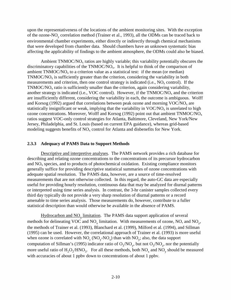
Various research studies have used aloft measurements (aircraft, ozonesondes) of ozoneand precursors to characterize transport. Figures 2-2 and 2-3 provide examples of aircraftmeasurements made during the 1995 NARSTO-Northeast study. Above approximately 400 to600 m elevation, ozone concentrations were ~80 ppbv within spirals flown between 0400 and0700 EST. Thus, substantial concentrations of ozone were available over an extended region forcarryover into the daytime. These data also show that in the air aloft, ozone levels had reachedtheir maximum potential—the air masses were aged and had too little NOx to sustain furtherozone production after sunrise. However, at the urban locations, ozone levels below ~400 mwere depleted relative to concentrations aloft, and the presence of higher concentrations of NOyimplied that ozone had been depleted by reaction with fresh emissions of NO. With sunrise,sufficient NOx was present to then generate much higher ozone concentrations, as indicated bythe maximum potential ozone values in Figures 2-2 and 2-3, though of course these higherconcentrations would be diminished following vertical mixing with air aloft having ozoneconcentrations of ~80 ppbv.

When aloft ozone or precursor measurements are combined with measurements of windspeeds and velocities, estimates of ozone transport across flux planes are possible. Exampleapplications include Roberts et al. (1994) and Blumenthal et al. (1997).

Tracer studies are also useful for characterizing atmospheric transport; in addition, tracersare used to quantify dispersion characteristics of plumes, providing empirical data for evaluatinglong-range trajectory models and conducting material balances for use in quantitative sourceapportionment. Both planned tracer releases, using inert, nondepositing gases such as sulfurhexafluoride (SF6) or perfluorocarbons, and tracers of opportunity have been used. Atmospherictransport studies are logistically less demanding than other types of tracer applications sincedocumentation of tracer locations and travel times typically suffices to meet the objectives ofsuch studies (Rappolt and Teuscher , 1995). Caution must be exercised in inferring transportdistances because the deposition rates of the pollutants of interest exceed those of the tracers bymany orders of magnitude. Planned tracer releases have been used to qualitatively track thetransport of pollutants from the Los Angeles metropolitan area into the Mojave Desert (Reible etal., 1982), from a power plant south of Las Vegas into Arizona (Green, 1998), within the LosAngeles area (Horrell et al., 1989), and from sources near ground level compared with tall stacks(Englund et al.,1989). During the 1990 San Joaquin Valley Air Quality Study (SJVAQS),perfluorocarbon tracer releases revealed transport from the San Francisco Bay areaapproximately 250 km down the length of the San Joaquin Valley (Rappolt and Quon, 1995).The SJVAQS operated 72 tracer monitoring sites within a domain of approximately

2-16

0.0

50.0

100.0

150.0

200.0

250.0

Con

cent

ratio

n (p

pbv)

0 200 400 600 800 1000 1200 1400 1600 1800 2000Elevation (m)

Overwater spiral June 19, 1995 morning flight 0700

New Haven June 19, 1995 morning flight 0500

0.0

50.0

100.0

150.0

200.0

250.0

Con

cent

ratio

n (p

pbv)

0 200 400 600 800 1000 1200 1400 1600 1800 2000Elevation (m)

0.0

50.0

100.0

150.0

200.0

250.0

Con

cent

ratio

n (p

pbv)

0 200 400 600 800 1000 1200 1400 1600 1800 2000Elevation (m)

Brookhaven June 19, 1995 morning flight 0400

Measured ozone

Measured ozone

Measured ozone

Maximum potential ozone estimated from measured NOy



Figure 2-2. Aloft ozone concentrations on the morning of June 19, 1995 at three locations.The maximum potential ozone concentrations were predicted using the methodof Blanchard et al. (1999). Data were obtained by STI aircraft. Source:Blanchard, 1998.

2-17

New Haven July 14, 1995 morning flight 0500

0.0

50.0

100.0

150.0

200.0

250.0

Con

cent

ratio

n (p

pbv)

0 200 400 600 800 1000 1200 1400 1600 1800 2000Elevation (m)

0.0

50.0

100.0

150.0

200.0

250.0

Con

cent

ratio

n (p

pbv)

0 200 400 600 800 1000 1200 1400 1600 1800 2000Elevation (m)

Brookhaven July 14, 1995 morning flight 0400

Overwater spiral July 14, 1995 morning flight 0700

0.0

50.0

100.0

150.0

200.0

250.0

Con

cent

ratio

n (p

pbv)

0 200 400 600 800 1000 1200 1400 1600 1800 2000Elevation (m)

Measured ozone

Measured ozone

Measured ozone




Figure 2-3. Aloft ozone concentrations on the morning of July 14, 1995 at three locations.The maximum potential ozone concentrations were predicted using the methodof Blanchard et al. (1999). Measurements were made by STI aircraft. Source:Blanchard, 1998.

2-18

150 km x 250 km (Rappolt and Teuscher, 1995); the 72 sites provided density sufficient forrevealing atmospheric transport distances, transport times, and the relative magnitudes oftransported versus fresh emissions (Smith and Lehrman, 1995).

Two recent analyses of ozone or precursor transport using PAMS data are documented inthe draft PAMS data usage report (U.S. Environmental Protection Agency, 2000).


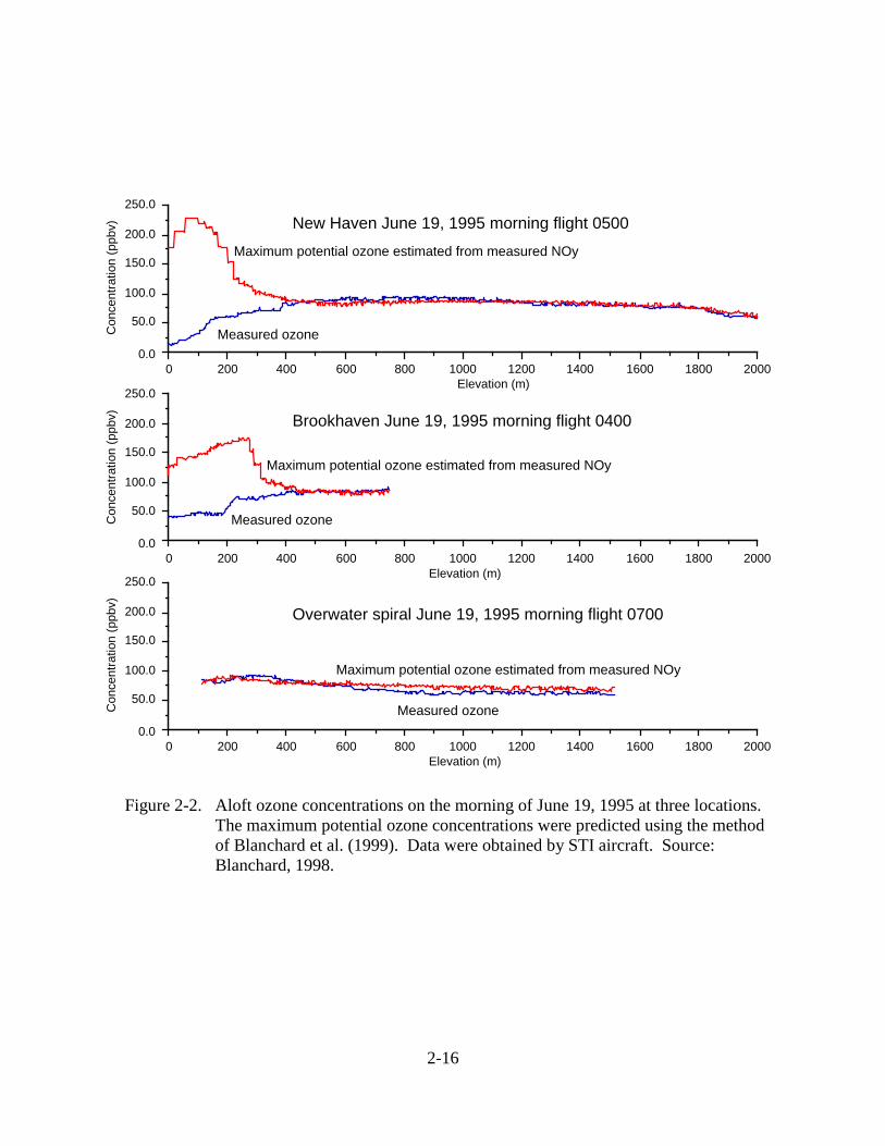
Transport analyses using either surface or aloft data generally cannot be carried out in aroutine manner; typically, such analyses require a substantial amount of interpretation, time, andeffort.

Planned tracer studies are expensive and provide limited temporal coverage. In contrast,tracers of opportunity sometimes provide temporally extensive data sets at low cost. However,neither planned tracers nor tracers of opportunity can provide quantitative assessment of therelative magnitudes of transported and locally generated ozone. The reason for this limitation isthat tracers do not have the same deposition rates or rates of chemical reaction as do ozone or itsprecursors, so quantitative estimation of transport contributions is not possible. Tracers ofopportunity are rare, and PAMS data do not provide measurements of species that might besuitable as unique tracers.


Transport analyses generally rely upon meteorological data from a fairly extensivenetwork of stations. The PAMS surface measurements can contribute to the surfacemeteorological databases. To date, studies have not shown that PAMS species data provide anytracers of opportunity.

Aloft ozone measurements are not incorporated into the PAMS network, nor into otherroutine monitoring networks. PAMS upper-air meteorological data are a valuable resource forinterpreting variations of surface-level concentrations. At present, these data are not asaccessible as they could be, nor are the measurements compiled and reviewed uniformly.


Upper-air meteorological measurements are valuable and should be continued. It wouldbe of great value to implement improvements in validation, data access, and the tools availablefor using the upper-air data. Aloft measurements of ozone may be acquired during specialresearch studies.

2-19

2.5 PROVIDING DATA FOR MODEL APPLICATION AND EVALUATION


Four principal methods have been employed for evaluating modeling accuracy:performance evaluation, sensitivity analysis, diagnostic evaluation, and corroborating analyses.PAMS data potentially can contribute to both performance evaluation and diagnostic evaluation.In addition, PAMS data can be used for conducting complementary corroborating analyses usingtechniques such as delineating VOC and NOx limitation.

Performance evaluation is the process of comparing model predictions to observedambient data. For Eulerian models, comparisons of predictions to observations are complicatedby an important incommensurability: model predictions are concentration averages over thedimensions of a grid cell, whereas ambient measurements are concentrations recorded at aspecific location and time. Thus, perfect agreement is not expected. The existence of multiplemonitoring stations within the dimensions of a typical model grid cell (i.e., 4-5 km horizontalscale) is helpful for characterizing the variability across stations. When the predicted ozonevalues of urban- and regional-scale Eulerian models have been compared with ozonemeasurements, mean errors of about 35% have been typical, along with biases of about 5% to15%, usually toward underprediction of ozone peaks

A more demanding test of model performance than comparing predicted and measuredozone concentrations is to compare predicted and observed concentrations of precursor species,such as NO, NO2, TNMOC, or some hydrocarbon or carbonyl species. Because precursorspecies are not monitored as extensively as is ozone, past comparisons of predicted andmeasured precursor concentrations have been limited, but they typically revealed discrepancieson the order of 30% to 50% (Roth et al., 1989). PAMS measurements provide a rich databasewith which to test model applications more thoroughly.

Performance evaluation, through comparison of predicted and measured concentrations,is necessary but not sufficient for evaluating model accuracy. A serious limitation of modelperformance evaluation is that predicted and measured species concentrations may agreereasonably well if compensating errors exist. Thus, additional tests are needed. Modelevaluation typically also includes sensitivity analysis, which is the process of determining amodel’s response, or sensitivity, to variations in key model inputs, parameters, or equations.One approach to sensitivity analysis is to simply alter input or parameter values, rerun the model,and determine the effects. Model sensitivities to variations of input or parameter values can alsobe determined more directly through several mathematical techniques. The primary procedurethat has been used in photochemical air quality models is known as the direct decoupled method(Dunker, 1981, 1984). This method has been applied to identify the sensitivity of the predictedmixing ratios of ozone and other species to uncertainties in the rate constants and stoichiometriccoefficients of the chemical reactions used in a gas-phase chemical mechanism (Gao et al.,1995a, 1995b). Sensitivity analyses typically do not require ambient measurements, so PAMSdata are not critical for this aspect of model testing.

2-20

A third approach to model evaluation employs techniques for diagnostic evaluation ofsimulations. Diagnostic evaluations typically examine the capacity of a model application toreproduce a variety of atmospheric processes that are thought to substantially influence ambientpollutant concentrations. Emphasis is placed on designing tests to reveal flaws in the model, ifpresent. For example, a performance evaluation protocol (Roth et al., 1998) developed for anEulerian modeling application (SARMAP) to central California (Chang et al., 1997; Lu andChang, 1998) establishes a series of diagnostic steps, beginning with a review of the scientificformulation of the model and concluding with comparisons to other modeling studies. A keystep is the evaluation of individual components of the model, which is accomplished through aseries of three emissions-related tests, thirteen meteorological tests, and eight air-quality tests.

One recent photochemical model evaluation using PAMS data is documented in the draftPAMS data usage report (U.S. Environmental Protection Agency, 2000).


Thorough performance and diagnostic evaluation of a model, or modeling system,requires substantial effort and commitment of the necessary resources. When completed, themodeling system is expected to be of known reliability and capable of providing levels ofaccuracy commensurate with its intended uses. In practice, such a rigorous evaluation process ismore comprehensive in scope and consumptive of time and effort than the process typicallyadopted for use. Schedule, financial, and technical resource constraints usually limit the abilityto carry out some aspects of the evaluation program. In this regard, it appears unrealistic todesign the PAMS network around a complete set of model evaluation needs. However, some ofthe data required for model evaluation may be acquired within the existing PAMS protocol, orwith modest changes, and at reasonable program cost.


A complete model evaluation process normally requires data that can only be acquiredduring special field studies. Routine measurements, including those of the PAMS network,should be considered as a supplement to the more extensive databases that are designedspecifically for model evaluation.

The EPA Office of Research and Development (ORD) has recently identified a set ofmeasurements needed for diagnostic model evaluation (Table 2-2). The EPA then comparedthese measurement needs with available PAMS data. Three changes to the PAMS measurementprotocol were considered possible: (1) addition of some continuous formaldehyde monitors,(2) addition of NO2-specific monitors, and (3) addition of some high-sensitivity (ppbv detectionlimits) CO monitors. These recommendations are consistent with recommendations derivedfrom consideration of other uses of the PAMS data. In addition, for performance and diagnosticmodel evaluation, maintaining hydrocarbon speciation at as many Type 2 and Type 3 sites aspossible would be highly desirable. Note that other PAMS data analyses do not necessarilyrequire speciation at all Type 3 sites. The measurement of other species, such as HNO3, H2O2,HONO, OH or nitrate radicals, and other compounds, was considered useful from a modelingperspective but too expensive or difficult to do on a routine basis.

Table 2-2. EPA ORD priorities for use of PAMS data for model evaluation (reproduced from ORD memo).

Priority Locations Recommended Parameters Reason For Need

1 All sites NO2NOy (with preference of NO2 over NOy if forced tochoose one or the other)NOO3speciated VOC*Total NMHC

To check ratios over time as the characterof the atmosphere changes due to controlsand other forces

HCHO (formaldehyde–continuous/short term)

H2O2 (1 hr routinely, but capability in special study toachieve 5 minute average)

To check on regime change and style ofO3 production

2 Selected sites

PANs (n-PAN, PPN, total PAN); HNO3 To track trends over time

3 Special sites H2O

4 Special sites CO (need to determine which PAMS sites also have COmonitors)–need ppb resolution, however

5 Special sites Other VOC compounds (e.g., oxygen-containingcompounds)

Needed for other model mechanismtesting

6 Special sites Other aldehydes–if high enough (surface reactions onparticles?)

*VOCs needed for aging studies–27 VOCs for emission check purposes; some of those and another 10 (total of 37) needed for diagnostics. Data needed downwind ofdowntown. ORD expressed concern about dropping compounds even at upwind and downwind sites for aging study purposes.PAN = peroxyacetylnitratePPN = peroxypropionylnitrate

2-21

2-22

One of the stated PAMS objectives is to provide hydrocarbon measurements appropriatefor evaluating the initial or boundary conditions of modeling studies. However, regional, andeven urban-scale, modeling studies all locate the model domain boundaries far upwind of themain areas of study. PAMS Type 1 sites typically are not close to model boundaries. Thus, theusefulness of PAMS data for constraining model boundary concentrations appears limited.


Type 3 sites should be reviewed for replacement of carbonyl measurements withcontinuous formaldehyde monitors. NO2-specific monitors should be added to some Type 3 sitesand the usefulness of the data evaluated. High-sensitivity (ppbv detection limits) CO monitorsshould be added to Type 2 and Type 3 sites. VOC speciation should be maintained at Type 2and Type 3 sites.

2.6 FORECASTING EPISODES


Ozone forecasting has typically relied upon analyses of meteorological data to predict theoccurrence of conditions conducive to ozone formation. In part, synoptic analyses have beenused to identify, for example, the locations of high pressure systems or blocking ridges. Indifferent parts of the country, various specific measured or derived meteorological quantitieshave been found useful as predictors of high-ozone days. Such quantities include upper-airtemperatures, certain pressure gradients, or other indicators of stagnation conditions. Recently,some forecasting techniques applied to the Atlanta area have made use of pinene and selectedolefin concentrations. Morning concentrations of other species may also prove useful. Anotherrecent approach has been to use the Urban Airshed Model (UAM) to forecast next-day peakozone concentrations (Chang and Cardelino, 2000). In general, most forecasting approaches arelikely to rely primarily on analysis of meteorological conditions. The availability of real-timesounding data will aid such methods. Such data are also needed for UAM forecasting if thatapproach proves feasible.


Enable real-time access to PAMS auto-GC and surface and upper-air meteorological data.

2.7 OTHER USES OF PAMS DATA

PAMS data potentially are useful for purposes that are auxiliary to the original objectivesof the network, including

• characterizing ambient air toxics for exposure modeling and trend analyses, • characterizing emissions and ambient concentrations of nitrogen species, • providing data for evaluation of particulate matter, and • enhancing special studies.

2-23

To be most useful for these other purposes, further consideration should be given to thetypes of measurements made and the time periods sampled. For example, ambient toxicassessment realistically requires year-round measurements. Typical sampling routines involvecollection of 24-hr samples once every 6 or 12 days throughout the year. Other samplingregimens are employed for studies of PM. Potentially, PAMS speciated VOC measurementsmight provide research-level information relevant to the formation of secondary organic carbonaerosol. Further assessment is needed. Conversely, measurements of elemental carbon, typicallyincluded within sampling of PM, could be useful in VOC receptor modeling for distinguishingdiesel from gasoline exhaust if they were carried out with adequate time resolution (hourly ormulti-hour).

Two recent analyses of air toxics exposure using PAMS data are documented in the draftPAMS data usage report (U.S. Environmental Protection Agency, 2000).

3-1

3. RECOMMENDATIONS

In reviewing the literature, we have prepared general recommendations for the PAMSnetwork and specific recommendations for the Northeast and Mid-Atlantic PAMS sites. Theserecommendations should be considered preliminary as we have not yet completed our analysesof the data. We suggest these recommendations be used as a place from which to begindiscussions and analyses.

3.1 GENERAL RECOMMENDATIONS FOR THE PAMS NETWORK

3.1.1 Number of sites of each type1. Examine the possibility of eliminating speciated hydrocarbon sampling at the second

Type 2 site in many large cities. Preliminary data analyses suggest that in many cities,source composition is similar at both Type 2 sites, so little new information is beinggenerated from speciated hydrocarbon measurements at the second site. However, itwould generally be useful to maintain monitoring of ozone, NO, NOx, and CO at thesecond Type 2 site, depending upon the existing spatial density of monitoring. Ifspeciated hydrocarbon measurements are discontinued at Type 2A sites, optionallyreplace speciated hydrocarbon sampling with continuous total NMHC (+/- 10 ppbC at50 ppbC). The continuous measurements are less resource-intensive and yieldinformation on primary pollutant emission levels and changes over time, the spatialdistribution of which is valuable to understand.

2. Maintain a long and continuous data record with good data quality and a high level ofdata completeness at one or a few sites; this record is more important than broad spatialcoverage for the purpose of trend analysis. However, the representativeness of sitesrequires assessment. A good example is the possibility of opposing trends at some Type2 and Type 3 sites. In some areas, Type 2 sites may have experienced declining levels ofozone precursors. However, downwind sites may have experienced less or no change inprecursor levels as suburban growth counterbalanced emission controls. Sufficientspatial coverage is needed to capture all trends.

3. Maintain a sufficient density of monitoring sites with measurements of ozone, NO, andNOx in areas between Type 2 and Type 3 sites so that the transition from VOC to NOxlimitation, which typically occurs somewhere in the near-to-far downwind area, could beidentified to within 10 km. This recommendation pertains more to the whole compliancenetwork than to PAMS sites. Nonetheless, it is an important design consideration.

3.1.2 Species measured at each site1. Measure NO2 and NOy at Type 3 and Type 4 PAMS sites with +/- 1 ppbv in the range

1 to 10 ppbv. In addition, maintain a conventional NOx measurement at all sites duringsome periods, and at some sites continuously, to facilitate comparison with NOx datafrom other monitoring sites.

3-2

2. Add high sensitivity (ppbv detection limits) hourly CO monitors to PAMS Type 2 orType 2A sites for aiding the evaluation of emission inventories.

3. Add high sensitivity (ppbv detection limits) hourly CO monitors to PAMS Type 3 sitesfor assessing the loss rates of NOx and NOy and improving evaluations of the relationshipbetween ozone formation and NOx levels.

4. Standardize upper-air meteorological measurement reporting and make data more widelyaccessible.

5. Add semivolatile measurements to Type 2 sites on the morning of every sixth day, or addcontinuous elemental or black carbon measurements, to better estimate the dieselemissions contributions.

6. Eliminate use of the Nafion dryer, if possible, to allow expansion of the PAMS target listto include more species such as pinenes and to improve accuracy of measurements ofC2-C6 alkenes, including isoprene.

7. Replace some Type 3 or Type 4 monitors with continuous total NMHC (+/- 10 ppbC at50 ppbC). Collocate continuous NMHC and speciated measurements for a sufficienttime to establish a relationship. Then use occasional canisters to check speciation.

8. Tailor the PAMS target species list to permit summing of closely related compounds.For some groups of compounds, summing could improve the accuracy of values close todetection limits and eliminate possible misidentification of close peaks. Candidatecompounds for summing are (1) 2,2-dimethylpentane, 2-methylpentane, and 3-methylpentane, (2) o-, m-, and p-ethyl toluenes, and (3) o-, m-, and p-diethyl benzenes.

9. Consider “lumping” C2 and C3 compound concentrations at selected sites to simplify theanalytical demands.

3.1.3 Frequency and resolution of measurements1. Reduce carbonyl measurement requirements to afternoon samples at downwind sites and

morning samples at Type 2 sites. Expand the list of carbonyls measured to be morecomplete (including heavier carbonyls) OR use continuous formaldehyde monitors atselected sites.

2. Eliminate or reduce measurements at some Type 3 or Type 4 sites.

3.2 SPECIFIC RECOMMENDATIONS FOR THE NESCAUM AND MARAMAREGIONS—PRELIMINARY AND CONTINGENT UPON COMPLETION OFDATA ANALYSES

Based on the general recommendations of Section 3-1, we provide a set of specificrecommendations for the PAMS monitors in the NESCAUM and MARAMA regions. Theserecommendations are presented for consideration and further evaluation by NESCAUM. Theyare not intended to be final, nor are they meant to be implemented without careful review of alltheir implications by NESCAUM, MARAMA, EPA, and other parties involved with the PAMSnetwork.

3-3

3.2.1 Number of sites of each type1. Review site typing. Preliminary analysis of the PAMS data suggests that some sites

exhibit characteristics similar to sites of other types (see Table 3-1). Therecommendations that follow should be reconsidered upon review of the existing sitetypes.

2. If further data analyses reveal highly similar hydrocarbon speciation between Type 2 and2A sites in some areas, consider eliminating speciated hydrocarbon sampling at Type 2Asites: Long Island MA, Hamden CT, Queens Com. College NY, Living Classroom MD,Camden NJ, Ft. Lee School VA. Consider if any of these Type 2A sites provide morerepresentative data than the Type 2 sites. Maintain ozone and NOx or NOy monitors.Optionally replace speciated hydrocarbon sampling with continuous NMHC.

3. Review AIRS for coverage near Type 3 sites and in downwind suburban and rural areas.Within each of the PAMS urban domains, add NOx or NOy monitors to three to sixdownwind suburban or rural compliance monitoring locations where ozone is presentlymeasured.

3.2.2 Species, frequency, and resolution of measurements at each site1. Add NO2 and/or NOy instrumentation at the following Type 3 sites: Newbury MA,

Stafford CT, Borderland MA, Ware MA, Sherwood Island CT, Aldino MD, RiderCollege NJ, and Fort Meade MD. Add NO2 and/or NOy to the existing NOxinstrumentation at the following Type 4 sites: Acadia ME, Cape Elizabeth ME, TruroMA, New Brunswick NJ. In the NESCAUM area, all Type 3 and Type 4 sites exceptNewbury now have NOy. Maintain existing NOx instruments, or add them wherepossible, to allow comparisons between NOx and NOy.

2. Add high-sensitivity (ppbv detection limits) hourly CO monitors to the following PAMSType 2 and Type 2A sites: Lynn MA, Long Island MA, Bronx NY, Queens CommunityCollege NY, Kittery ME, East Providence RI, Chicopee MA, McMillan Reservoir DC,Essex MD, Clifton Park MD, Living Classroom MD.

3. Add high-sensitivity (ppbv detection limits) hourly CO monitors to PAMS Type 3 sites:Newbury MA, Stafford CT, Borderland MA, Ware MA, Sherwood Island CT, AldinoMD, Rider College NJ, and Fort Meade MD.

4. Replace some Type 3 or Type 4 monitors with continuous total NMHC (+/- 10 ppbC at50 ppbC). Type 3 sites are Newbury MA, Stafford CT, Borderland MA, Ware MA,Sherwood Island CT, Aldino MD, Rider College NJ, and Fort Meade MD. Type 4 sitesare Acadia National Park ME, Cape Elizabeth ME, Truro MA, and Lums Pond DE. Useoccasional canisters to check speciation. Consider lumping C2 and C3 compounds wherespeciation is done.

5. Install continuous formaldehyde instruments at Type 2 (Lynn MA, Long Island MA,Bronx NY, Queens Community College NY, Kittery ME, East Providence RI, ChicopeeMA, McMillan Reservoir DC, Essex MD, Clifton Park MD, Living Classroom MD) andType 3 sites (Newbury MA, Stafford CT, Borderland MA, Ware MA, Sherwood IslandCT, Aldino MD, Rider College NJ, and Fort Meade MD). If continuous formaldehyde

3-4

monitors are installed, reduce cartridge measurement requirements to occasional spotchecks with afternoon samples at Type 3 sites and morning samples at Type 2 sites. Ifspot checks are done, expand the list of carbonyls measured to be more complete (heaviercarbonyls) at Type 3 and Type 4 sites; eliminate expanded carbonyl sampling at Type 2sites (data analyses to date indicate that formaldehyde is an adequate predictor ofacetaldehyde, and higher carbonyls are present at low concentrations).

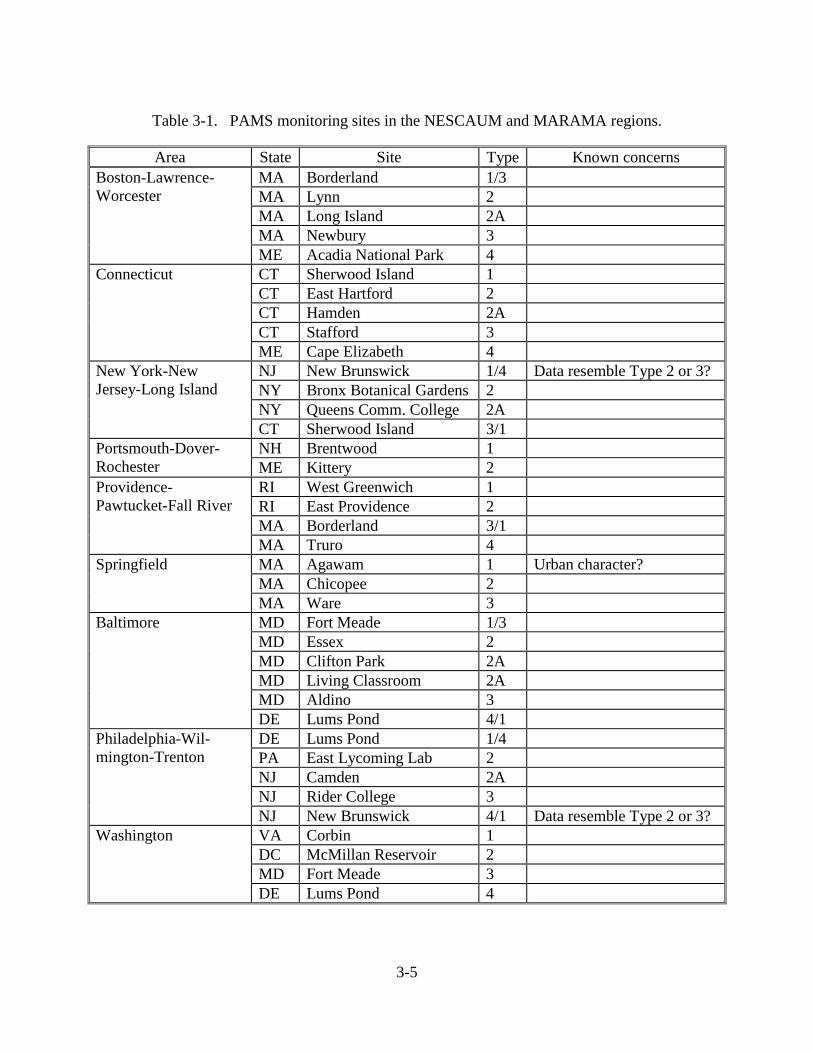
3-5

Table 3-1. PAMS monitoring sites in the NESCAUM and MARAMA regions.

Area State Site Type Known concernsMA Borderland 1/3MA Lynn 2MA Long Island 2AMA Newbury 3

Boston-Lawrence-Worcester

ME Acadia National Park 4CT Sherwood Island 1CT East Hartford 2CT Hamden 2ACT Stafford 3

Connecticut

ME Cape Elizabeth 4NJ New Brunswick 1/4 Data resemble Type 2 or 3?NY Bronx Botanical Gardens 2NY Queens Comm. College 2A

New York-NewJersey-Long Island

CT Sherwood Island 3/1NH Brentwood 1Portsmouth-Dover-

Rochester ME Kittery 2RI West Greenwich 1RI East Providence 2MA Borderland 3/1

Providence-Pawtucket-Fall River

MA Truro 4MA Agawam 1 Urban character?MA Chicopee 2

Springfield

MA Ware 3MD Fort Meade 1/3MD Essex 2MD Clifton Park 2AMD Living Classroom 2AMD Aldino 3

Baltimore

DE Lums Pond 4/1DE Lums Pond 1/4PA East Lycoming Lab 2NJ Camden 2ANJ Rider College 3

Philadelphia-Wil-mington-Trenton

NJ New Brunswick 4/1 Data resemble Type 2 or 3?VA Corbin 1DC McMillan Reservoir 2MD Fort Meade 3

Washington

DE Lums Pond 4

4-1

4. REFERENCES

PAMS ProgramBortnick S.M., Coutant B.W., Holdcraft J.R., Boehm R., Ma Z.J., and Holdren M.W. (2001)

Photochemical assessment monitoring stations (PAMS): data assessment. Final technicalreport prepared for U.S. Environmental Protection Agency, Office of Air QualityPlanning and Standards, Research Triangle Park, NC by Battelle, Columbus, OH,Contract No. 68-D98-030, January. Also available at<http://www.nescaum.org/committees/pams.html>.

STAPPA/ALAPCO (2000) Draft recommendations from a PAMS workshop sponsored by EPA,State, and Territorial Air Pollution Program Administrators and the Association of LocalAir Pollution Control Officials, Las Vegas, NV, March.

U.S. Environmental Protection Agency (2000) Draft PAMS data usage report (a cross tabulationof PAMS data in studies/analyses, 1999-2000. Prepared by U.S. EnvironmentalProtection Agency, Office of Air Quality Planning and Standards Emissions Monitoringand Analysis Division, Research Triangle Park, NC, November.

TrendsBlanchard C.L. (2000) Methods for attributing ambient air pollutants to emission sources.

Annual Review of Energy and the Environment 24, 239-265.

Bloomfield P.R, Steinberg L.J., and Yang Q. (1996) Accounting for meteorological effects inmeasuring ozone levels and trends. Atmos. Environ. 30, 3067-3077.

Box G.E.P. and Tiao G.C. (1975) Intervention analysis with applications to economic andenvironmental problems. JASA 70, 70-79.

Cassmassi J.C. and Bassett M.E. (1993) Air quality trends in the South Coast Air Basin. InSouthern California Air Quality Study Data Analysis: Proceedings of an InternationalSpecialty Conference, Pittsburgh PA: Air and Waste Management Association, pp. 27-32.

Chock D.P., Kumar S., and Hermann R.W. (1982) An analysis of trends in oxidant air quality inthe south coast air basin of California. Atmos. Environ. 16, 2615-2624.

Cox W.M. and Chu S. (1993) Meteorologically adjusted ozone trends in urban areas: aprobabilistic approach. Atmos. Environ. 27B, 425-434.

Curran T.C. and Frank N.H. (1991) Ambient ozone trends using alternative indicators. In:Tropospheric Ozone And The Environment: Papers From an International SpecialtyConference, Los Angeles, CA March 19-22, 1990. Berglund R.L., Lawson D.R., andMcKee D.J., eds., Air and Waste Management Association, Pittsburgh, PA, pp. 749-759.

Fiore A.M., Jacob D.J., Logan J.A., and Yin J.H. (1998) Long-term trends in ground level ozoneover the contiguous United States, 1980-1995. J. Geophys. Res. 103(D1), 1471-1480.

4-2

Fujita E. (1993) Trends in emissions and ambient concentrations of CO, NMHC and NOx in theSouth Coast Air Basin. In Proceedings of an International Specialty Conference:Southern California Air Quality Study Data Analysis, Air and Waste ManagementAssociation, Pittsburgh, PA, pp. 43-48.

Kolaz D.J. and Swinford R.L. (1990) How to remove the influence of meteorology from theChicago area ozone trend. Paper no. 90-97.5 presented at the 83rd Annual Meeting andExhibition of the Air & Waste Management Association, June 24-29, 1990.

Korsog P.E. and Wolff G.T. (1991) An examination of tropospheric ozone trends in thenortheastern U.S. (1973-1983) using a robust statistical method. Atmos. Environ. 25B,47-57.

Kuntasal G. and Chang T.Y. (1987) Trends and relationships of O3, NOx and HC in the SouthCoast Air Basin of California. J. Air Pollut. Control Assoc. 37, 1158-1163.

Main H.H., Roberts P.T., and Reiss R. (1998) Analysis of photochemical assessment monitoringstation (PAMS) data to evaluate a reformulated gasoline (RFG) effect. Final reportprepared for U.S. Environmental Protection Agency, Office of Mobile Sources,Washington, DC by Sonoma Technology, Inc., Santa Rosa, CA, STI-997350-1774-FR2,April. Also available at <http://epa.gov/oar/oaqps/pams/rfg-oms.pdf>.

MARAMA (1997) 1995 ozone atlas for the Mid Atlantic region. Mid-Atlantic Regional AirManagement Association, Baltimore, MD, June.

Milanchus M.L., Rao S.T., and Zurbenko I.G. (1998) Evaluating the effectiveness of ozonemanagement efforts in the presence of meteorological variability. J. Air & Waste Manag.Assoc. 48, 201-215.

Rao S.T. and Zurbenko I.G. (1994) Detecting and tracking changes in ozone air quality. J. Air &Waste Manag. Assoc. 44, 1089-1092.

Rao S.T., Porter P.S., Zurbenko I.G., Dunker A.M., and Wolff G.T. (1999) Ozone air qualityover North America: a critical review of trend detection techniques and assessments.NARSTO Critical Review Paper, <http://www.cgenv.com/Narsto>.

Shively T.S. (1991) An analysis of the trend in ground-level ozone using non-homogeneouspoisson processes. Atmos. Environ. 25B, 387-395.

Sirois A. (1993) Temporal variation of sulphate and nitrate concentrations in precipitation inEastern North America: 1979-1990. Atmos. Environ. 27A, 945-963.

Stoeckenius T. (1991) Adjustment of ozone trends for meteorological variation. In:Tropospheric Ozone And The Environment: Papers From an International SpecialtyConference, Los Angeles, CA March 19-22, 1990. Berglund R.L., Lawson D.R., andMcKee D.J., eds., Air and Waste Management Association, Pittsburgh, PA, pp. 781-800.

U.S. Environmental Protection Agency (2000) National Air Quality and Emissions TrendsReport, 1998. U.S. Environmental Protection Agency, Research Triangle Park, NC,<http://www.epa.gov/oar/aqtrnd98>.

4-3

Weatherhead E.C., Reinsel G.C., Tiao G.C., Meng X.L., Choi D., Cheang W.K., Keller T.,DeLuisi J., Wuebbles D.J., Kerr J.B., Miller A.J., Oltmans S.J., and Frederick J.E. (1998)Factors affecting the detection of trends: Statistical considerations and applications toenvironmental data. J. Geophys. Res. 103, 17149-17161.

Zeldin M.D., Cassmassi J.C., and Hoggan M. (1991) Ozone trends in the South Coast Air Basin:an update. In Tropospheric Ozone And The Environment: Papers From an InternationalSpecialty Conference, Los Angeles, CA, March 19-22, 1990. Berglund R.L., LawsonD.R., and McKee D.J., eds., Air and Waste Management Association, Pittsburgh, PA,pp. 760-771.

Inventory accuracy – Top-down evaluationChinkin L.R., Funk T.H., Main H.H., and Roberts P.T. (1999) PAMS data analysis for Southern

California, Volume VI: Use of PAMS data to evaluate a South Coast Air Basin emissioninventory. Report prepared for South Coast Air Quality Management District, DiamondBar, CA by Sonoma Technology, Inc., Petaluma, CA, STI-997528-1916-FR, November.

Lurmann F.W. and Main H.H. (1992) Analysis of the ambient VOC data collected in theSouthern California Air Quality Study. Report prepared for the California Air ResourcesBoard, Sacramento, CA by Sonoma Technology, Inc., Santa Rosa, CA, STI-99120-1161-FR, Contract No. A823-130, February.

Main H.H. and Roberts P.T. (1993) Validation and analysis of the Lake Michigan Ozone Studyambient VOC data. Draft final report prepared for Lake Michigan Air DirectorsConsortium, Des Plaines, IL by Sonoma Technology, Inc., Santa Rosa, CA, STI-90217-1352-DFR, April.

Main H.H., Hurwitt S.B., and Roberts P.T. (1999) Spatial and temporal characteristics ofCalifornia PAMS and long-term trend site VOC data (1990-1997). Final report preparedfor U.S. Environmental Protection Agency, Research Triangle Park, NC by SonomaTechnology, Inc., Petaluma, CA, STI-998241-1883-FR, May.

Main H.H., Alcorn S.H., and Roberts P.T. (1999) Characteristics of volatile organic compoundsin the mid-Atlantic region. Final report prepared for MARAMA, Baltimore, MD, bySonoma Technology, Inc., Petaluma, CA, STI-998484-1869-FR2, November.

Stoeckenius T. and Jimenez M. (2000) Reconciliation of an emissions inventory with PAMSambient monitoring data in the Mid-Atlantic states. Revised final report prepared forMARAMA, Baltimore, MD, by ENVIRON International Corporation, Novato, CA undersubcontract to E.H. Pechan & Associates, Springfield, VA, May.

Inventories - Receptor ModelingFujita E.M., Watson J.G., Chow J.C., and Lu Z. (1994) Validation of the chemical mass balance

receptor model applied to hydrocarbon source apportionment in the Southern CaliforniaAir Quality Study. Environ. Sci. Technol. 28, 1633-1649.

Fujita E.M., Watson J.G., Chow J.C., and Magliano K. (1995) Receptor model and emissionsinventory source apportionments of nonmethane organic gases in California’s SanJoaquin Valley and San Francisco Bay area. Atmos. Environ. 29, 3019-3035.

4-4

Scheff P.A., Wadden R.A., Bates B.A., and Aronian P.F. (1989) Source fingerprints for receptormodeling of volatile organics. J. Air Pollut. Control Assoc. 39, 469-478.

Scheff P.A. and Wadden R.A. (1993) Receptor modeling of volatile organic compounds. 1.emission inventory and validation. Environ. Sci. Technol. 27, 617-625.

Scheff P.A., Wadden R.A., Kenski D.M., Chung J., and Wolff G. (1996) Receptor modelevaluation of the southeast Michigan Ozone Study ambient NMOC measurements. J. Air& Waste Manag. Assoc. 46, 1048-1057.

Tombach I. (1982) Application of receptor modeling to volatile organic compounds. In:Receptor Models Applied To Contemporary Pollution Problems: APCA SpecialtyConference Proceedings. Air and Waste Management Association, Pittsburgh, PA,pp. 338-347.

Watson J.G. (1982) Overview of receptor model principles. In Receptor Models Applied ToContemporary Pollution Problems: APCA Specialty Conference Proceedings. Air andWaste Management Association, Pittsburgh, PA, pp. 6-17.

Watson J.G. (1997) Observational models: the use of chemical mass balance methods.Presented at U.S. Environmental Protection Agency Source Attribution Workshop,Research Triangle Park July 16-18, 1997.

Watson J.G., Chow J.C., and Fujita E.M. (1999) Review of volatile organic compound sourceapportionment by chemical mass balance. NARSTO Critical Review Paper,<http://www.cgenv.com/Narsto>.

Interpretive Data AnalysesCarter W.P.L. and Atkinson R. (1987) An experimental study of incremental hydrocarbon

reactivity. Environ. Sci. Tech. 21, 670-679.

Chaemides W.L. et al. (2000) An assessment of tropospheric ozone pollution – A NorthAmerican perspective, <http://www.cgenv.com/Narsto>.

Hales J.M., Gery M.W., and Crouse R. (1993) VOC reactivity and its application to emissionregulation. American Petroleum Institute, Washington, DC.

Roberts P.T., Main H.H., and Hurwitt S.B. (1999) Technical assistance to MARAMA on EPAcumulative exposure project (CEP): review of air toxics modeling. Final report preparedfor MARAMA, Baltimore, MD, by Sonoma Technology, Inc., Petaluma, CA,STI-998561-1853-FR, January.

Vukovich FM. (2000) Weekday/weekend differences in OH reactivity with VOCs and CO inBaltimore, Maryland. J. Air & Waste Manag. Assoc. 50, 1843-1851.

Delineation of VOC and NOx LimitationBlanchard C.L. (1998) Analysis of data from the 1995 NARSTO-Northeast Air Quality Study:

observation-driven methods for delineating VOC and NOx limitation. Prepared forCoordinating Research Council, Atlanta, GA, March.

4-5

Blanchard C.L., Lurmann F.W., Roth P.M., Jeffries H.E., and Korc M. (1999) The use ofambient data to corroborate analyses of ozone control strategies. Atmos. Environ. 33,369-381.

Blanchard C.L. (2000) Ozone process insights from field experiments - Part III: Extent ofreaction and ozone formation. Atmos. Eviron. 34, 2035-2043.

Blanchard C.L., Roberts P.T., Chinkin L.R., and Roth P.M. (1995) Application of smogproduction (SP) algorithms to the Coastal Oxidant Assessment for Southeast Texas(COAST) data. Paper 95- TP15P.04 presented at the Air and Waste ManagementAssociation 88th Annual Meeting and Exhibition, San Antonio, Texas, June 18-23.

Cardelino C.A. and Chameides W.L. (1995) An observation-based model for analyzing ozoneprecursor relationships in the urban atmosphere. J. Air & Waste Manag. Assoc. 45, 161-180.

Chang T.Y. and Rudy S.J. (1993) Ozone-precursor relationships: a modeling study of semi-empirical relationships. Environ. Sci. Tech. 27, 2213-2219.

Chang T.Y. and Suzio M.J. (1995) Assessing ozone-precursor relationships based on a smogproduction model and ambient data. J. Air & Waste Manag. Assoc. 45, 20-28.

Chang T.Y., Chock D.P., Nance B.I., and Winkler S.L. (1997) A photochemical extent parameterto aid ozone air quality management. Atmos. Environ. 2787-2794.

Jacob D.J., Horowitz L.W., Munger J.W., Heikes B.G., Dickerson R.R., Artz R.S. and KeeneW.C. (1995) Seasonal transition from NOx- to hydrocarbon- limited conditions for ozoneproduction over the eastern United States in September. J. Geophys. Res. 100(D5), 9315-9324.

Lu C.H. and Chang J.S. (1998) On the indicator-based approach to assess ozone sensitivities andemissions features. J. Geophys. Res. 103(D3), 3453-3462.

Milford J.B., Gao D., Sillman S., Blossey P., and Russell A.G. (1994) Total reactive nitrogen(NOy) as an indicator for the sensitivity of ozone to NOx and hydrocarbons. J. Geophys.Res. 99(D2), 3533-3542.

Sillman S, He D., Cardelino C., and Imhoff R. E. (1997) The use of photochemical indicators toevaluate ozone-NOx-hydrocarbon sensitivity: case studies from Atlanta, New York, andLos Angeles. J. Air & Waste Manag. 47, 1030-1040.

Sillman S. (1995) The use of NOy, H2O2, and HNO3 as indicators for ozone-NOx-hydrocarbonsensitivity in urban locations. J. Geophys. Res. 100(D7), 14175-14188.

Trainer M, Parrish D.D., Buhr M.P., Norton R.B., Fehsenfeld F.D., Anlauf K.G., BottenheimJ.W., Tang Y.Z., Wiebe H.A., Roberts J.M., Tanner R.L., Newman L., Bowersox V.C.,Meagher J.F., Olszyna K.J., Rodgers M.O., Wang T., Berresheim H., Demerjian K.L. andRoychowdhury U. K.. (1993) Correlation of ozone with NOy in photochemically aged air.J. Geophys. Res. 98, 2917-2926.

Wolff G.T. and Korsog P.E. (1992) Ozone control strategies based on the ratio of volatileorganic compounds to nitrogen oxides. J. Air & Waste Manag. Assoc. 42, 1173-1177.

4-6

TransportBlanchard C.L. (1998) Analysis of data from the 1995 NARSTO-Northeast Air Quality Study:

observation-driven methods for delineating VOC and NOx limitation. Prepared forCoordinating Research Council, Atlanta, GA, March.

Blumenthal D.L., Lurmann F.W., Roberts P.T., Main H.H., MacDonald C.P., Knuth W.R., andNiccum E.M. (1997) Three-dimensional distribution and transport analyses forSJVAQS/AUSPEX. Final report prepared for the San Joaquin Valley Air Pollution StudyAgency, Sacramento, CA by Sonoma Technology, Inc., Santa Rosa, CA, Technical andBusiness Systems, Santa Rosa, CA, and California Air Resources Board, Sacramento,CA, STI-91060-1705-FR, February.

Englund W.G., Teuscher L.H., and Marsh S. (1989) Perfluorocarbon tracer experiments duringthe Southern California Air Quality Study of 1987. Paper no. 89-138.1 presented at the82nd Annual Meeting and Exhibition of the Air and Waste Management Association,Anaheim, CA, June 25-30.

Green M. (1998) The Project MOHAVE tracer study: study design, data quality, and overviewof results. Desert Research Institute, Las Vegas, NV, 89119.

Horrell R.S., Deem M., Wyckoff P., Shair F., and Crawford N. (1989) Ground release SF6 tracerexperiments used to characterize transport and dispersion of atmospheric pollutantsduring the Southern California Air Quality Study of 1987. Paper no. 89-138.2 presentedat the 82nd Annual Meeting and Exhibition of the Air and Waste ManagementAssociation, Anaheim, CA, June 25-30.

Rappolt TJ and Quon SL. 1995. Inert tracer gas measurements. In:SJVAQS/AUSPEX/SARMAP 1990 Air Quality Field Measurement Project. SolomonP.A. and Thuillier R. H., eds., Pacific Gas and Electric Company, San Ramon, CA, Vol.II, pp. 8-1 to 8-63.

Rappolt T.J. and Teuscher L.H. (1995) Identification of regional air mass transport using tracerstudies. In Proceedings, Regional Photochemical Measurement and Modeling Studies,Volume I: Results and Interpretation of Field Measurements. Ranzieri A.J. and SolomonP.A., eds., Air and Waste Management Association, Pittsburgh, PA, pp. 166-180.

Reible D.D., Ouimette J.R., and Shair F.H. (1982) Atmospheric transport of visibility degradingpollutants into the California Mojave Desert. Atmos. Environ. 16, 599-613.

Roberts P.T., Dye T.S., Korc M.E., and Main H.H. (1994) Air quality data analysis for the 1991Lake Michigan Ozone Study. Final Report prepared for Lake Michigan Air DirectorsConsortium, Des Plaines, IL by Sonoma Technology, Inc., Santa Rosa, CA, STI-92022-1410-FR, September.

Roberts P.T., Dye T.S., Ray S.E., Anderson J.A., Blumenthal D.L., MacDonald C.P., Main H.H.,and Kumar N. (1999) Analysis of data from the 1995 NARSTO-Northeast StudyVolume V: Three-dimensional analysis of aircraft and upper-air meteorological data.Report prepared for Coordinating Research Council, Atlanta, GA, under subcontract toENVIRON International Corp., Novato, CA by Sonoma Technology, Inc., Petaluma CA,STI-95426-1836-FR, April.

4-7

Smith T.E. and Lehrman D.E. (1995) Long-range tracer studies in the San Joaquin Valley. InProceedings, Regional Photochemical Measurement and Modeling Studies, Volume I:Results and Interpretation of Field Measurements. Ranzieri A.J. and Solomon P.A., eds.,Air and Waste Management Association, Pittsburgh, PA, pp. 151-165.

Model Performance EvaluationChang J.S., Jin S., Li Y., Beauharnois M., Lu C.H., Huang H.C., Tanrikula S., and DaMassa J.

(1997) The SARMAP Air Quality Model. California Air Resources Board, Sacramento,CA.

Demerjian K.L., Roth P.M., and Blanchard C.L. (1995) A new approach for demonstratingattainment of the ambient ozone standard: modeling, analysis, and monitoringconsiderations. U.S. Environmental Protection Agency, Research Triangle Park, NC,EPA/600/R-96/134.

Dunker A.M. (1981) Efficient calculation of sensitivity coefficients for complex atmosphericmodels. Atmos. Environ. 15, 1155-1161.

Dunker A.M. (1984) The decoupled direct method for calculating sensitivity coefficients inchemical kinetics. J. Chem. Phys. 81, 2385-2393.

Gao D., Stockwell W.R., and Milford J.B. (1995a) First-order sensitivity and uncertaintyanalysis for a regional-scale gas-phase chemical mechanism. J. Geophys. Res. 100,23153-23166.

Gao D., Stockwell W.R., and Milford J.B. (1995b) Global uncertainty analysis of a regional-scale gas-phase chemical mechanism. J. Geophys. Res. 101, 9107-9119.

Lu C.H. and Chang J.S. (1998) On the indicator-based approach to assess ozone sensitivites andemissions features. J. Geophys. Res. 103, 3453-3462.

Roth P.M., Blanchard C.L., and Reynolds S.D. (1989) The role of grid-base, reactive air qualitymodeling in policy analysis: perspectives and implications, as drawn from a case study..U.S. Environmental Protection Agency, Research Triangle Park, NC, EPA/600/3-89/082.

Roth P.M., Reynolds S.D., Blanchard C.L., Chang J., Jin S., Magiano K., Seaman N., TanrikulaS., and Tesche T.W. (1998) Protocol for Evaluating the Performance of the SARMAPModel. California Air Resources Board, Sacramento, CA.

ForecastingChang M.E. and Cardelino C. (2000) Application of the Urban Airshed Model to forecasting

next-day peak ozone concentrations in Atlanta, GA. J. Air & Waste Manag. Assoc. 50,2010-2024

Documents

LITERATURE REVIEW IN SUPPORT OF PAMS PROGRAM ASSESSMENT › projects › regional-pams-assessment › nescaum … · LITERATURE REVIEW IN SUPPORT OF PAMS PROGRAM ASSESSMENT FINAL