Limit cycle bifurcations in resonant LC power inverters

Nonlinear Dynamics manuscript No.(will be inserted by the editor)

Limit cycle bifurcations in resonant LC power inverters under zerocurrent switching strategy

Luis Benadero · Enrique Ponce · Abdelali El Aroudi · Francisco Torres

Received: date / Accepted: date

Abstract The dynamics of a DC-AC self-oscillating LC res-onant inverter with a zero current switching strategy is con-sidered in this paper. A model that includes both the seriesand the parallel topologies and accounts for parasitic resis-tances in the energy storage components is used. It is foundthat only two reduced parameters are needed to unfold thebifurcation set of this extended system: one is related to thequality factor of the LC resonant tank and the other accountsfor the balance between serial and parallel losses. Througha rigorous mathematical study, a complete description of thebifurcation set is obtained and the parameter regions wherethe inverter can work properly is emphasized.

Keywords Piecewise linear dynamics · Limit cycles ·Bifurcations · Power inverters · ZCS control

E. Ponce and F. Torres are partially supported by the Spanish Ministe-rio de Economía y Competitividad, in the frame of project MTM2015-65608-P and by the Consejería de Economía y Conocimiento de laJunta de Andalucía under grant P12-FQM-1658. L. Benadero and A.El Aroudi were supported by the Spanish Ministerio de Ciencia e In-novación under grant DPI2013-47293-R.

L. BenaderoDepartament de FísicaUniversitat Politècnica de Catalunya, Barcelona, SpainE-mail: [email protected]

E. PonceDepartamento de Matemática AplicadaEscuela Técnica Superior de Ingeniería, Sevilla, SpainE-mail: [email protected]

A. El AroudiGAEI Research group, Departament d’Enginyeria Electrònica, Elèc-trica i AutomàticaUniversitat Rovira i Virgili, Tarragona, SpainE-mail: [email protected]

F. TorresDepartamento de Matemática AplicadaEscuela Técnica Superior de Ingeniería, Sevilla, SpainE-mail: [email protected]

1 Introduction

Resonant inverters were introduced many years ago althoughtheir use has been confined for a long time to very specificapplications, such as in high-voltage power supplies or au-dio amplifiers [1–3]. With the introduction of new regula-tions concerning efficiency and power density, power elec-tronics designers have been pushed to find increasingly moreefficient conversion systems. As a consequence, a renewedinterest has emerged in resonant conversion. In particular,resonant inverters have recently gained more popularity inemerging applications such as wireless power transfer [4–6],battery charging in electrical vehicles [7], induction heat-ing [8] and powering high intensity discharge lamps [9],among others.

Roughly speaking, resonant inverters are systems thatinclude a switching network and a resonant LC tank circuitthat converts a DC voltage into an AC voltage, thus provid-ing AC power to a load. To do so, the switching networktypically generates a square-wave signal that is applied toa resonant tank circuit. The switching frequency in reso-nant converters is usually very close to the resonant tankfrequency and therefore the AC amplitude of the state vari-ables is larger than the ripple of PWM hard switching con-verters. Furthermore, by rectifying and filtering the AC out-put of a resonant inverter, resonant DC-DC converters canbe formed.

Different types of resonant inverters exist and these areclassified according to the type of switching network, theconfiguration of the resonant tank circuit, and the number ofthe energy storage components. The parallel resonant con-verter (PRC) and the series resonant converter (SRC) areexamples of topologies with two energy-storage elements[10, 11], corresponding to the simplest possible configura-tions.

2 Luis Benadero et al.

A major advantage of resonant inverters is their ability tooperate with zero voltage switching (ZVS) or with zero cur-rent switching (ZCS) [12]. These techniques help to min-imize switching losses even when inverters work at highswitching frequency, hence allowing the use of small stor-age components. Therefore, the power density is improved.Another benefit is the low electromagnetic interference thatappears in resonant topologies.

Regarding the physical realization of resonant inverters,a serious problem for designers comes from the lack of arigorous analysis accounting for the dynamical behavior andthe stability of oscillations. That is why in the majority of thereported works, the results are not general and can only beapplied to particular cases. The purpose of this paper is toprovide a sound approach to deal with this problem and toget a deep insight into the dynamics of these systems.

A rather general piecewise linear (PWL) model includ-ing parasitic resistances for energy storage elements consid-ering both parallel and series design is introduced in thispaper. We assume a ZCS control and study thoroughly thedynamics that can be obtained depending on the choice ofdifferent parameters. For that, we derive a canonical modelwith only two parameters: one of them is related to the qual-ity factor of the LC circuit while the other accounts for thebalance between serial and parallel losses. The two extremevalues of this second parameter address to the ideal seriesand the parallel cases. The bifurcation set is obtained throughthe rigorous mathematical description of the different bi-furcation curves. The parameter region where the invertershould work for a proper operation is emphasized.

The study of PWL systems can be a difficult task thatis not within the scope of traditional analysis techniques fornonlinear systems. In particular, a sound bifurcation theoryis lacking for such systems due to their nonsmooth character,and so their study must be done case by case e.g., [13, 14].Enforced by modern nonlinear engineering problems, someworks in the literature on planar PWL systems deal with vec-tor fields where continuity at the boundary is not assumed.

Dealing with non-smooth systems, after the pioneeringwork of Filippov [15], many efforts have been devoted totheir bifurcation and stability analysis. One-parameter bi-furcations for these systems are throughly studied in [16].In particular, some specific cases are considered in [17–19].In [20], it was shown that when there exists a generalizedsingular point of pseudo-focus type, degenerate Hopf bifur-cations are possible. Later, other studies analyzing pertur-bations of systems in the so-called focus-focus (FF) caseappeared. For instance, the possible existence of two smalllimit cycles under general perturbations of FF systems thatcan move the equilibrium points out of the boundary is re-ported in [21]. The number of bifurcating limit cycles in-creases when the two involved subsystems share the linearpart of focus type and different quadratic terms are consid-

iL

S1

+

−

L

vC

+

−

S2

S3 S4

+

−

Vg

C rcp

to S1 and S4

to S2 and S3

δ

δ

rcs

rls

Rop

Ros

iL

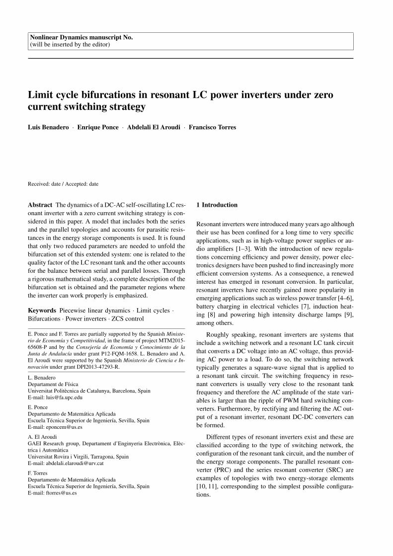
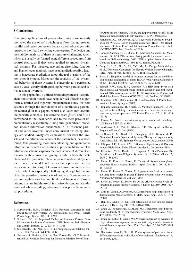
Fig. 1 Generalized schematic diagram of an LC resonant inverter.Here, some extra elements have been included to account for both par-allel and series resonant converters ans also for parasitic elements. Notethat if a resistor is missing, either its corresponding conductance or re-sistance vanishes.

ered, see [22], or even more when the linear terms do notcoincide, see for instance [23] and the references therein.

Restricting our attention to discontinuous PWL systemswith two zones separated by a straight line, some works havebeen done. In particular, in [24] a similar situation to the oneappearing in our model is considered, namely systems witha global vector field symmetrical with respect to the origin.

In this paper, a planar discontinuous PWL dynamicalsystem with symmetry and two linear zones is obtained tomodel a self-oscillating LC resonant inverter. At the discon-tinuity line a repulsive sliding set exists that plays a key rolein some limit cycle bifurcations. It is shown that the bound-aries of attraction of the existing equilibrium points are de-termined by unstable closed loops. The bifurcation pattern,which includes a saddle-node bifurcation of limit cycles, isextensively analyzed, getting a valuable information for thecorrect operation and design of the inverter.

The rest of the paper is organized as follows. In Section2, the mathematical model of the proposed general inverteris obtained and some canonical forms are derived in order tominimize the number of parameters for its analysis. Section3 is devoted to the complete determination of the bifurcationset regarding the two essential parameters previously intro-duced. In Section 4, some qualitative features regarding os-cillations are stressed and the safety region of the circuit ishighlighted. Finally, some concluding remarks are summa-rized in the last section.

2 System description and mathematical modeling

2.1 System Description

Figure 1 shows a generalized circuit diagram of a resonantDC-AC H-bridge inverter. In this diagram, some extra el-ements have been included in such a way that both paralleland series resonant converters can be studied. Also, parasiticresistances in the energy storage elements are taken into ac-count. In that diagram, the output series resistance Ros; the

Bifurcations in LC resonant inverters under ZCS strategy 3

inductor with inductance L and parasitic series resistor rls;the output parallel conductance Gop = 1/Rop; and the capac-itor with capacitance C with parasitic parallel conductancegcp = 1/rcp and parasitic series resistance rcs can be identi-fied. Other elements in the circuit diagram in Fig. 1 are theinput source voltage Vg, and the switches S1, S2, S3 and S4.

The circuit operation is based on an automatically ac-tivated switching between two configurations driven by thesignals δ and δ = 1− δ . The switches S1 and S4 are ONwhen iL > 0 (therefore δ = 1), and they are turned OFFwhen iL < 0 (δ = 0), where iL is the current through theinductor L. The switches S2 and S3 are respectively drivenin a complementary way to S1 and S4, so that a ZCS controlis implemented.

It is clear that without switching, the capacitor voltageand the inductor current tend to some constant values. Inother words, when δ = 1 there is always an equilibriumpoint with positive values for the capacitor voltage and theinductor current and when δ = 0 there is another equilibriumpoint with negative values for those magnitudes.

The goal of the switching control is to take advantage ofthe transient regimes associated to these equilibria. Then, bybuilding a suitable aggregation of orbits, a limit cycle, whichis the desired oscillating behavior in steady state regime, ismade up. This goal will be possible only under certain re-strictions, as shown later. Even when the switching is acting,the dynamics could be addressed to one of these equilibriumpoints depending on the starting conditions, which is unde-sirable. For instance, if the quality factor of the LC circuit islower than a critical value to be determined later, the normalzero initial condition lies on the attraction basin of the un-desired equilibria and therefore the limit cycle would not bereached. On the contrary, an appropriate choice of parame-ters will warrant a good performance for the inverter understandard initial conditions. Such a choice of parameters onlycan be soundly made after an analysis of all the possible dy-namics in the circuit. As an important feature to be fulfilled,the attraction basin of these equilibria should be minimizedas much as possible to get a robust operation for the inverter.

2.2 State-space model

Let vC be the voltage of the capacitor C and recalling iL is thecurrent in the inductor L, then, by applying Kirchoff voltageand current laws, we get

iL = ics +(icsrcs + vC)Gop,

uVg = LdiLdt

+ iL(Ros + rls)+ icsrcs + vC,

where ics, that is the current through rcs, is

ics =CdvC

dt+gcpvC.

After some algebra, the following model is obtained

ddt

(vCiL

)= A

(vCiL

)+ub, (1)

where

A =

−Gp

Cκ

C

−κ

L−Rs

L

, b =

0Vg

L

,

and the factor κ is introduced to define the equivalent seriesresistance Rs and the equivalent parallel conductance Gp,

κ =1

1+ rcsGop

Rs = Ros + rls +κrcs, Gp = gcp +κGop.

The variable u = 2δ − 1 is determined by the control,such that u = 1 (that is, δ = 1) if iL > 0, and u = −1 (thatis, δ = 0) if iL < 0. This control strategy based on the useof the sign of the inductor current in the switching decisionis called zero current switching (ZCS). Then, the switchingcondition, which is in general a function of the state vari-ables and time, depends only on the inductor current and itcan be expressed in terms of the state variables as

h(vC, iL) = iL, (2)

so that the ZCS control strategy leads to u = sign(h(vC, iL))and the system is autonomous.

Next, in order to simplify the analysis of its possible dy-namics and bifurcations, system (1)-(2) will be normalizedinto a simpler form with a minimum number of parameters.

2.3 Canonical forms

In this section, we will obtain the Frobenius or rational canon-ical form for the common linear part, which is well suitedfor our subsequent analysis. Doing so, the needed changesof variables preserve the discontinuity line, so that the sec-ond variable is still associated to the electrical current acrossthe inductance. Note that in general, if we choose instead theJordan canonical form, then the discontinuity line should notcoincide with any of the coordinate axes.

First, we consider the natural frequency ω0 and the qual-ity factor Q of the two linear subsystems in (1),

ω0 =√

det(A) =

√RsGp +κ2

LC,

1Q

=− tr(A)

ω0=

Gp

ω0C+

Rs

ω0L,

(3)


where det(A) and tr(A) stand for the determinant and thetrace of matrix A, respectively. Also, we introduce a param-eter β defined as

β =QGp

ω0C= 1− RsQ

ω0L=

GpLGpL+CRs

, (4)

where all the equivalent expressions for β come from (3).It is worth noting that 0≤ β ≤ 1. The case β = 0 arises

when Gp = 0, and it corresponds to the ideal series inverter,i.e., the resistors Gop and rcp are absent. The case β = 1arises when Rs = 0, i.e., the resistors Ros, rls and rcs are ab-sent and it corresponds to the ideal parallel inverter.

In searching for a canonical form, the state vector is re-defined by using the change of variables

x =

(x1x2

)=

κ

Vg−LGp

CVg

0ω0LVg

( vCiL

),

and the independent variable is changed by using a new timeτ = ω0t so that the following proposition is obtained.

Proposition 1 System (1)-(2) can be reduced to

dxdτ

= Ax+ub, (5)

h(x) = x2, (6)

where matrix A and vector b are redefined as

A =

0 1

−1−1Q

, b =

−β

Q1

,

and u = 1 if h(x)> 0 or u =−1 if h(x)< 0.

According to (6), the switching manifold Σ is defined as

Σ = {(x1,x2) : x2 = 0},

and so the state space of the canonical form has two linearityregions, namely

Σ+ = {(x1,x2) : x2 > 0}, Σ

− = {(x1,x2) : x2 < 0}.

The system (5), with a constant switch variable u, hasthe two equilibria

x± =±(x1,x2) =±(

1− β

Q2 ,β

Q

),

where it is assigned x+ and x− to u = 1 and u = −1 re-spectively. Whenever β > 0, since x2 > 0, we deduce thatx+ ∈ Σ+ and x− ∈ Σ−, so both equilibria are real. However,if β = 0 (the ideal series inverter case), then the two equi-libria are located at the points x± =±(1,0) ∈ Σ , that is theylie at the switching line.

For these new variables the natural frequency is the unityand the poles p± of system (5), that is, the eigenvalues ofmatrix A, are

p± =− 12Q±√

14Q2 −1.

Here, two different cases appear depending on the valueof the quality factor Q. If Q ≤ 1/2 then the eigenvalues arereal and negative, so that equilibria are stable nodes. On theother hand, if Q > 1/2 then both eigenvalues are complexwith negative real part, that is, equilibria are stable foci. Inthe piecewise smooth system (5)-(6) with the parameter con-dition β = 0, the node-focus transition at the value Q = 1/2gives rise to a non smooth bifurcation to be studied later.

When Q≤ 1/2 the equilibria have some invariant mani-folds associated to the real eigenvalues, so that orbits cannotcut such invariant manifolds. As a consequence, any trajec-tory can cross the switching manifold Σ at most once, pre-cluding the oscillatory dynamics.

When Q > 1/2, oscillatory dynamics can appear. Theeigenvalues of matrix A given in (5) are now

p± =− 12Q± i

√1− 1

4Q2 = σ ± iν .

Note that these eigenvalues are located on the unit circle be-cause σ2 + ν2 = 1. Then it turns out more convenient tostudy the dynamical behavior of our system by means of anew parameter γ which is associated to the focus contrac-tion when γ < 0 or the focus expansion when γ > 0. Theparameter γ will be crucial to study the bifurcations of sys-tem (1)-(2) and it is introduced as follows,

γ =σ

ν=

−1√4Q2−1

< 0. (7)

Notice that as γ < 0, the focus is contractive. We are then inposition of stating the following result.

Proposition 2 Assuming Q > 1/2, system (1)-(2) can be re-duced to

dxdθ

= Ax+ub, (8)

h(x) = x2, (9)

where matrix A and vector b are redefined as

A =

(0 1+ γ2

−1 2γ

), b =

(2βγ

1

),

and u = 1 if h(x)> 0 or u =−1 if h(x)< 0.The system has two equilibria of focus type, with eigen-

values γ± i, namely

x± =±(

1− 4βγ2

1+ γ2 ,−2βγ

1+ γ2

). (10)


Proof For any value of parameter Q, system (1)-(2) can bereduced to (5)-(6). If Q > 1/2, the parameter γ in (7) is welldefined. Now, making in (5) the change of variables,

x1 = x1, x2 = νx2, θ = ντ,

dropping tildes and taking into account that

1+ γ2 =

1ν2 ,

1νQ

=−2γ,

system (8)-(9) is obtained. Equilibria computation is direct.

It is worth noting that if x(θ) is a solution of system(8)-(9), then −x(θ) is also a solution. As a consequence,an invariant closed curve Γ is either symmetric with respectto the origin or there exists another invariant closed curve Γ ′

which is the symmetrical one to Γ with respect to the origin.It must be emphasized that the reduced systems (5)-(6)

and (8)-(9) have only two parameters, Q and β , or γ andβ respectively. The parameters Q and γ are related to theglobal dissipation of the system while the parameter β canbe understood as the dissipation balance between series andparallel resistances.

In the following, we focus on the case Q > 1/2, and ac-cording to Proposition 2, we study system (8)-(9).

3 Sliding and crossing dynamics, limit sets andbifurcations

First, the sliding dynamics is studied; afterwards, the cross-ing dynamics and possible periodic orbits will be addressed.

3.1 Sliding set and pseudo equilibrium point

In accordance to the defined switching manifold Σ and thetwo corresponding state regions Σ+ and Σ−, system (8)-(9)can be rewritten as x = F(x), where

F(x) ={F+(x) =

(F+

1 (x),F+2 (x)

)= Ax+b, x ∈ Σ+,

F−(x) =(F−1 (x),F−2 (x)

)= Ax−b, x ∈ Σ−.

(11)

Orbits are well defined while they evolve without touch-ing the switching manifold Σ . To define the orbits arrivingat the discontinuity line Σ , we must distinguish between twodifferent possibilities. If the two vector fields point to thesame direction, we can concatenate solutions in a naturalway. On the contrary, when such normal components are inopposition, we adopt the Filippov convex method. In the se-quel, we will closely follow reference [16] to describe theFilippov method regarding system (11).

The product of the two normal components to the switch-ing manifold, at a point x = (x1,0) ∈ Σ is

(∇h(x)F+(x)) · (∇h(x)F−(x)) = F+2 (x)F−2 (x) = x2

1−1,

where ∇(·) is the gradient operator, and then

∇h(x) = (0,1),F+2 (x) =−x1 +1,F−2 (x) =−x1−1.

The crossing set Σ c ⊂ Σ is the set of all points x ∈ Σ ,where the normal components of F at both sides of the switch-ing manifold have the same sign, that is

Σc = {(x1,0) : |x1|> 1} .

At these points the orbits of system (11) cross the switchingmanifold Σ , i.e., orbits reaching Σ from one zone concate-nate in a natural way with orbits leaving Σ and entering theother zone.

The sliding set Σ s ⊂ Σ is the complement in Σ of thecrossing set Σ c, i.e.

Σs = {(x1,0) : |x1| ≤ 1},

which is the set of all points x ∈ Σ , where the normal com-ponents of the vector fields to the discontinuity line have op-posite sign or one of them vanishes. Note that F+

2 (x1,0) andF−2 (x1,0) do not simultaneously vanish at any point (x1,0).The sliding set is repulsive because for system (11),

F+2 (x)≥ 0 and F−2 (x)≤ 0, x ∈ Σ

s.

The Filippov method associates to every x ∈ Σ s the so-called sliding field Fs(x) by means of the convex combina-tion

Fs(x) = λF−(x)+(1−λ )F+(x),

where λ = λ (x) is selected so that Fs(x) is tangent to thesliding set, that is

∇h(x)Fs(x) = λ∇h(x)F−(x)+(1−λ )∇h(x)F+(x) = 0,

and then,

λ (x) =∇h(x)F+(x)

∇h(x)(F+(x)−F−(x))

For system (10), this implies

λ (x1) =F+

2 (x1,0)F+

2 (x1,0)−F−2 (x1,0)=

1− x1

2.

Therefore, for (x1,0) ∈ Σ s, the scalar differential equation

x1 = λF−1 (x1,0)+(1−λ )F+1 (x1,0) = 2βγx1 (12)

defines the so called sliding dynamics in the sliding set Σ s

for system (8)-(9).Solutions of (12) are called sliding solutions. In partic-

ular, constant sliding solutions are called pseudo-equilibria


of the system. When β = 0, equation (12) reduces to x1 = 0,and so every point in the sliding set is a pseudo-equilibriumpoint of system (11). When β > 0, the origin is the onlypseudo-equilibrium point. Taking into account that the slid-ing set Σ s is repulsive and that the origin is stable for thesliding dynamics, it turns out that system (11) has a pseudo-saddle at the origin for β > 0.

For system (11), the sliding set is delimited by the twopoints x±B = ±(1,0). If β > 0, then F+

2 (x+B ) = 0 and, re-calling that γ < 0, F−1 (x+B ) = 2βγ < 0. Moreover, since theorbit of the vector field F+ passing through x+B at a time, sayθ = θB, belongs to Σ+ for 0 < |θ − θB| < ε , the point x+Bis called a visible tangency point. Analogously, due to thesymmetry of the vector field, the point x−B = −(1,0) is alsoa visible tangency point.

Although the system is discontinuous, for any initial con-dition x(0), it is possible to define, both in forward and back-ward time, a unique solution Φ(θ ,x(0)), with Φ(0,x(0)) =x(0). Of course, assuming x(0)∈ Σ+ (x(0)∈ Σ− is symmet-rical), the corresponding solution Φ(θ ,x(0)) can be com-puted by solving x = F+(x) while x(θ) ∈ Σ+.

If a forward time solution x(θ) does not reach the switch-ing manifold Σ , it tends to the stable equilibrium x+. Oth-erwise, if the orbit reaches Σ at the point (x1(θ1),0) thennecessarily x1(θ1) ≥ 1. If x1(θ1) > 1, then the orbit entersΣ− and the vector field F− must be used to resume the com-putation. In the case x1(θ1) = 1, the system enters in slidingmode regime described by equation (12) and sliding takesplace for θ > θ1; if β > 0, this orbit tends toward the pseudo-saddle equilibrium at the origin and when β = 0, then it isassumed that x(θ) = x(θ1) = (1,0) for all θ > θ1.

In contrast, a backward time solution x(θ) always reachesthe discontinuity line Σ . Therefore, there exists a time θ2 < 0for which x(θ2) = (x1(θ2),0)∈ Σ , where x1(θ2)< 1. At thispoint, the following possibilities arise when θ < θ2.

(a) If β ≥ 0 and x1(θ2) < −1, the orbit crosses Σ and F−must be used to resume the reverse time computation.

(b) If β = 0 and−1≤ x1(θ2)< 1, then x(θ) = x(θ2) for allθ < θ2.

(c) If β > 0 and −1≤ x1(θ2)< 1, then the following casesarise(c1) If x1(θ2) = −1, then the orbit crosses Σ and then

follows in backward time the unique standard orbitin Σ− through the point x−B .

(c2) If−1< x1(θ2)< 0, then for θ < θ2, the orbit slidesin backward time towards the point x−B . Then, weproceed as in (c1).

(c3) If x1(θ2) = 0, then x(θ) = x(θ2) = (0,0) for allθ < θ2.

(c4) If 0 < x1(θ2)< 1, then the orbit slides towards thepoint x+B . Afterwards, the orbit follows in back-ward time the unique standard orbit in Σ+ throughthe point x+B .

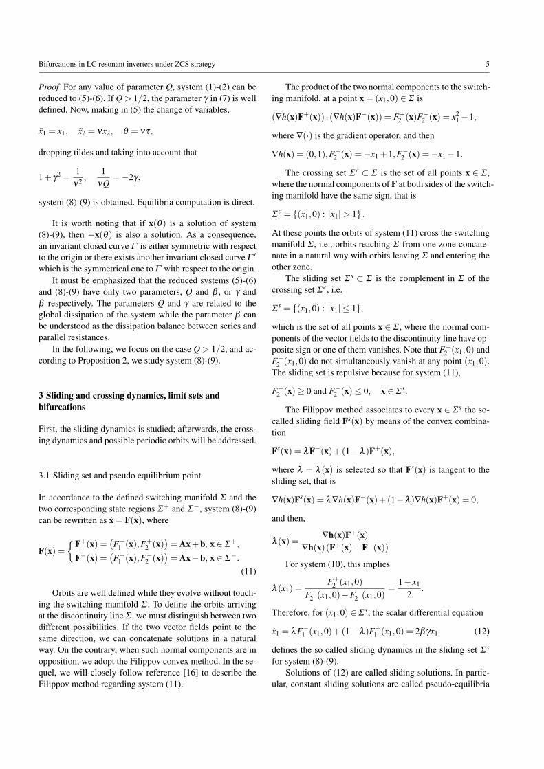
The different situations defined above are illustrated inFig. 2. Observe that excepting the orbits tangent to the switch-ing manifold Σ s at the points (±1,0), each panel can be ob-tained from the other one by reversing the sign of the arrows.Note also that system solutions are not invertible in the clas-sical sense, since the orbits can overlap on the sliding set,see [16].

3.2 Poincaré map associated to the switching manifold

Taking into account the symmetry of the vector field withrespect to the origin, we focus our attention on the upperhalf plane Σ+, where the system has an equilibrium point(x1,x2), see (10). Thus, by solving equation (8) with u = 1,it turns out(

x1(θ)− x1x2(θ)− x2

)= φ(θ)

(x1(0)− x1x2(0)− x2

), (13)

where φ(θ) is the evolution operator given by

φ(θ) = eγθ

(cosθ − γ sinθ (1+ γ2)sinθ

−sinθ cosθ + γ sinθ

).

We will resort to the auxiliary function

ϕγ(θ) = 1− eγθ (cosθ − γ sinθ), (14)

which was introduced in [13] and has the symmetry proper-ties

ϕ−γ(θ) = ϕγ(−θ), ϕ−γ(−θ) = ϕγ(θ), γ,θ ∈ R.

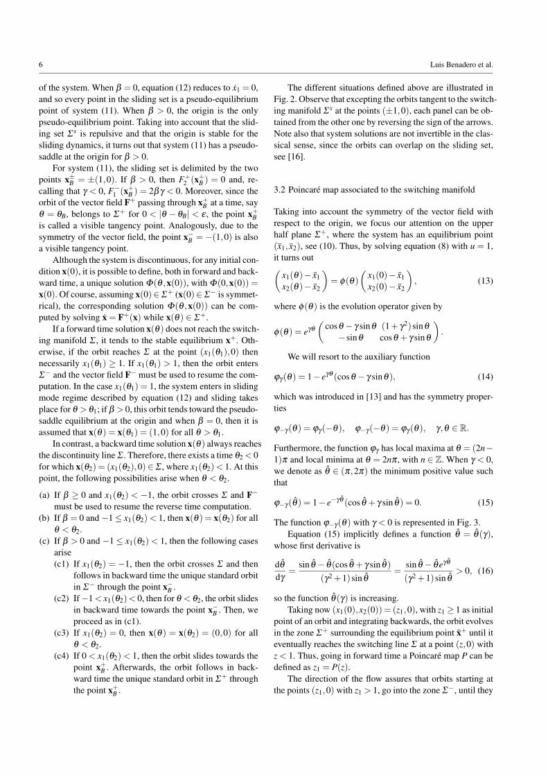
Furthermore, the function ϕγ has local maxima at θ = (2n−1)π and local minima at θ = 2nπ , with n ∈ Z. When γ < 0,we denote as θ ∈ (π,2π) the minimum positive value suchthat

ϕ−γ(θ) = 1− e−γθ (cos θ + γ sin θ) = 0. (15)

The function ϕ−γ(θ) with γ < 0 is represented in Fig. 3.Equation (15) implicitly defines a function θ = θ(γ),

whose first derivative is

dθ

dγ=

sin θ − θ(cos θ + γ sin θ)

(γ2 +1)sin θ=

sin θ − θeγθ

(γ2 +1)sin θ> 0, (16)

so the function θ(γ) is increasing.Taking now (x1(0),x2(0)) = (z1,0), with z1≥ 1 as initial

point of an orbit and integrating backwards, the orbit evolvesin the zone Σ+ surrounding the equilibrium point x+ until iteventually reaches the switching line Σ at a point (z,0) withz < 1. Thus, going in forward time a Poincaré map P can bedefined as z1 = P(z).

The direction of the flow assures that orbits starting atthe points (z1,0) with z1 > 1, go into the zone Σ−, until they


(a) Orbits in forward time. (b) Orbits in backward time.

Fig. 2 Orbits in a neighborhood of the sliding set when β > 0. Left panel: The sliding set is repulsive and the only two orbits entering the slidingset are the orbits arriving tangentially to the two points (±1,0). Right panel: In backward time the sliding set is attractive and orbits arriving atpoints (±x,0) with 0 < x≤ 1 leave the sliding set through the points (±1,0).

Fig. 3 Graph of function ϕ−γ (θ) with γ < 0. The value θ is definedby ϕ−γ (θ) = 0, with π < θ < 2π . The value θM is uniquely definedby ϕ−γ (−θM) = ϕ−γ (θM) or equivalently ϕγ (θM) = ϕγ (−θM), withπ < θM < θ .

reach Σ again at a point (z2,0) with z2 <−1. Therefore, wecan define another Poincaré map P as z2 = P(z1), for z1 > 1.

It is direct to see that when (P ◦P)(z) = z, a crossinglimit cycle exists and so, the crossing limit cycles corre-spond to fixed points of the map P◦P.

Assuming that P(z) = z1, we realize that the symmetryof the system imposes that P(−z) =−z1, and so

(P◦P)(z) =−P(−P(z)) = (−P)◦ (−P)(z).

Consequently, in looking for crossing limit cycles it issufficient to determine the points z < −1 such that P(z) =−z. Moreover, the derivative of the full Poincaré map P ◦Pat a fixed point z is

(P◦P)′(z) =−P′(−P(z))(−P′(z)) = (−P′(z))2,

hence, the fixed point is stable when |P′(z)|< 1 and unstablewhen |P′(z)|> 1.

Next the Poincaré map P is determined. Two cases arisesdepending on the value of β .

3.2.1 The case β = 0

When β = 0, the equilibrium point of the vector field F+ islocated at (1,0). Then, by solving equation (13), the Poincaré

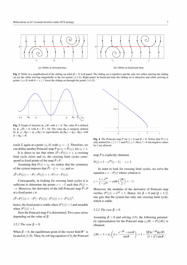
Fig. 4 The Poincaré map P for γ < 0 and β > 0. Notice that P(z) isonly defined for z≤ z < 1 and P(z)≥ 1. Here z > 0, but negative valuesfor z are allowed.

map P is explicitly obtained,

P(z) = 1− eγπ(z−1), z < 1.

In order to look for crossing limit cycles, we solve theequation z =−P(z) whose solution is

z =1+ eγπ

1− eγπ= coth

(γπ

2

)<−1.

Moreover, the modulus of the derivative of Poincaré mapverifies |P′(z)| = eγπ < 1. Hence, for β = 0 and Q > 1/2,one gets that the system has only one crossing limit cycle,which is stable.

3.2.2 The case β > 0

Assuming β > 0 and solving (13), the following paramet-ric representation for the Poincaré map z1(θ) = P(z(θ)) isobtained.

z(θ) = 1+ x2

(γ +

e−γθ − cosθ

sinθ

)= 1− 2βγe−γθ ϕγ(θ)

(1+ γ2)sinθ,


(17)

P(z(θ)) = 1+ x2

(γ− eγθ − cosθ

sinθ

)= 1+

2βγeγθ ϕ−γ(θ)

(1+ γ2)sinθ,

(18)

where π < θ ≤ θ , being ϕ−γ(θ) = 0. Obviously, variables zand P(z) also depend on parameters β and γ; such a depen-dence is made explicit only when it is oportune. The map Pis defined for z≤ z = z(θ)< 1, with P(z)≥ 1, and P(z)→∞

for z→−∞. An illustrative plot of the map P(z) is given inFig. 4.

Direct computations show that for π < θ ≤ θ , the twofirst derivatives of P are

P′(z) =− ϕγ(θ)

ϕγ(−θ)=

(z−1)e2γθ

P(z)−1< 0, (19)

P′′(z) =8β 2γ2(sinh(γθ)− γ sinθ)e3γθ

(1+ γ2)(P(z)−1)3 < 0. (20)

Moreover, when z→−∞, then θ → π and when z→ z, thenθ → θ . Therefore, we have

limz→−∞

P(z) = ∞, (21)

limz→−∞

P′(z) =−eγπ , limz→z

P′(z) =−∞. (22)

Now, we can state the following fact. For β > 0, sys-tem (11) can have at most two crossing limit cycles becausethe map P is concave down and so, its graph meets the sec-ondary diagonal at most in two points. The existence andstability of these crossing limit cycles are studied in Subsec-tion 3.4 after analyzing the closed curves containing the fullsliding set or a part of it.

3.3 The sliding invariant closed curves

Invariant closed curves containing points in the sliding setΣ s will be called sliding closed curves. Since orbits do notarrive at the repulsive sliding segment in forward time, theonly possible sliding invariant curves occur in backward timeand they must contain at least one of the tangency points.

When β = 0, from (12) every point in the sliding set is apseudo-equilibrium point and consequently sliding invariantclosed curves cannot exist.

To determine sliding limit cycles when β > 0, the orbitthrough the tangency point x+B = (1,0) is considered. Next,assuming γ < 0 and taking β as the bifurcation parameter,our interest is to compute the value of z, such that P(z) =1. From expression (18) the condition ϕ−γ(θ) = 0 must besatisfied, and so θ = θ , see (15). After some algebra, we get

z = P−1(1) = z(θ) = 1− 2βγ

γ + cot θ= 1− β

βhc(γ), (23)

where βhc(γ) is a function that can be defined as follows

βhc(γ) =12+

cot θ

2γ=

eγθ

2γ sin θ=

1

2(1− e−γθ cos θ). (24)

The equivalence among expressions in (24) comes from (15).Different scenarios can appear as it is shown in the next

proposition.

Proposition 3 Assuming γ < 0 in system (8)-(9), and takingβhc(γ) as in (24), the following statements hold.

(a) The function βhc(γ) is positive and increasing with γ .(b) If β = 0, then sliding limit cycles do no exist.(c) If 0 < β < βhc(γ), then there exists a symmetric pair of

unstable sliding limit cycles, each one of them living inonly one zone.

(d) If β = βhc(γ), then the above limit cycles become into asymmetric pair of unstable sliding homoclinic connec-tions to the origin.

(e) If βhc(γ) < β < 2βhc(γ), then there exists one unstablesliding limit cycle being symmetrical with respect to theorigin.

Proof The conditions π < θ < 2π and γ < 0 imply γ sin θ >

0, and then βhc > 0. Also, by computing the derivative

dβhc

dγ=

∂βhc

∂ θ

dθ

dγ+

∂βhc

∂γ,

we get

dβhc

dγ=

γ(θ − sin θ cos θ)− sin2θ

2eγθ sin θ(γ2 +1)(1− e−γθ cos θ)2,

and taking into account that θ − sin θ cos θ > 0, it is con-cluded that β ′hc(γ)> 0, and so βhc(γ) is increasing.

The orbit in backward time through the tangency pointx+B evolves in the region Σ+ and after surrounding the equi-librium point x+, arrives at the switching manifold at thepoint (z,0) and the following cases arise.

If β = 0, then the sliding set is full of pseudo-equilibriumwhat precludes the existence of any sliding motion.

If 0< β < βhc(γ), then from (23), it is found that 0< z<1. In this case, the orbit continues in backward time from thepoint (z,0) sliding towards the point x+B making one slidinginvariant closed curve. The symmetry imposes the existenceof another invariant closed curve on the other side of Σ .

When β = βhc(γ), then z = 0, i.e., the orbit arrives atthe pseudo-saddle located at the origin. Since the sliding dy-namics is repulsive towards the point x+B , there is a homo-clinic connection to the origin. The symmetry imposes theexistence of another homoclinic connection to the origin onthe other side of Σ .

When βhc(γ)< β < 2βhc(γ), then−1 < z < 0. From thepoint (z,0), the orbit continues sliding in backward time to-wards the tangency point x−B = (−1,0). Then the symmetry


imposes the closing of the orbit at the point x+B , making asliding limit cycle living in the two zones.

In any case, the invariant closed curve is unstable be-cause it contains a repulsive sliding segment.

3.4 The crossing limit cycles

In this section, the existence of crossing limit cycles is an-alyzed by fixing the parameter γ < 0 and taking β as thebifurcation parameter.

As shown before, crossing limit cycles are determinedby points z ≤ −1 satisfying P(z) = −z. Thus, they corre-spond to the zeros of the function

g(z) = z+P(z). (25)

The dependence for the function g of the parameters will besometimes emphasized by introducing the notation

g(z(θ ;β ,γ)) = z(θ ;β ,γ)+P(z(θ ;β ,γ)),

which from (17)-(18) can be written as,

g(z(θ ;β ,γ)) = 2− 4βγ

1+ γ2

(γ− sinh(γθ)

sinθ

). (26)

Next, some properties of the function g are established,see Fig. 5.

(a) The function g is defined for z ≤ z = P−1(1). Further-more, if z→−∞, then θ → π and from (26),

limz→−∞

g(z) =−∞.

In addition, taking into account (23), it is found

g(z) = z+P(z) = z+1 = 2− β

βhc(γ). (27)

(b) From (19)-(22) we deduce g′′(z)< 0 and so, the deriva-tive g′(z) monotonically decreases when −∞ < z < z,and furthermore,

limz→−∞

g′(z) = 1− eγπ > g′(z)> limz→z

g′(z) =−∞.

Since γ < 0, then 1− eγπ > 0, so that there exists onepoint zM(β ) with g′(zM(β )) = 1+P′(zM(β )) = 0. Thus,the function g is concave down and its maximum valueis g(zM(β )).

(c) Since the derivative of the Poincaré map P satisfies thecondition P′(zM(β )) = −1, the flight time θM ∈ (π, θ)

corresponding to the point zM(β ) is determined by therelation ϕγ(−θM)=ϕγ(θM), see (19) and Fig. 3, or equiv-alently by the equation

γ coth(γθM)− cotθM = 0. (28)

Note that γ coth(γθM)> 0, so that θM ∈ (π,3π/2). Then,the maximum value of function g is obtained by takingθ = θM in (26). Note that θM depends only on γ , so thatzM(β ,γ) = z(θM;β ,γ), see (17).

(d) It should be pointed out that

∂g(z(θ ;β ,γ))

∂β=−4γ

1+ γ2

(γ− sinh(γθ)

sinθ

)< 0. (29)

The function θM = θM(γ) which is implicitly definedfrom equation (28) has the first derivative

dθM

dγ=

2γθ − sinh(2γθ)

2sinh2(γθ)(1+ γ2)> 0,

and then the function θM(γ) is increasing. Also, from (28) itcan be shown that when γ →−∞, then θM → π and whenγ → 0, then θM tends to 4.493409..., which is the only rootof the equation θ cotθ = 1 in the interval (π,3π/2).

Since any crossing limit cycle is symmetric with respectto the origin, the minimum absolute value of its intersectionwith the switching manifold Σ is clearly 1, thus correspond-ing to a critical cycle that links the two endpoints x+B andx−B of the sliding set. Let this cycle be called critical cross-ing limit cycle (CC limit cycle, for short). For the sake ofconvenience, let us introduce the function

βcc(γ) = 2βhc(γ).

Now, the following results about crossing limit cyclesare given, see Fig. 5. Note that the new introduced valueβsn(γ) corresponds to the case when the maximum value offunction g vanishes.

Proposition 4 Assuming γ < 0 in system (8)-(9), there existsa positive function

βsn(γ) =(1+ γ2)sinθM

2γ (γ sinθM− sinh(γθM)), (30)

where θM is the only root of equation (28) in the interval(π,3π/2) such that

g(zM(βsn)) = 0

is satisfied and the following statements hold.

(a) The function βsn(γ) is positive and increasing with γ .(b) If β > βsn(γ) then there are no crossing limit cycles.(c) If β = βsn(γ) there exists one semi-stable crossing limit

cycle.(d) If βcc(γ)< β < βsn(γ) then there exist two crossing limit

cycles. The inner is unstable being the outer stable.(e) If β = βcc(γ) then there exist one unstable CC limit cy-

cle and one stable crossing limit cycle.(f) If β < βcc(γ) then there exists one stable crossing limit

cycle.

Proof Taking θ = θM and β = βsn in expression (26), theequality g(zM(βsn)) = 0 is obtained.


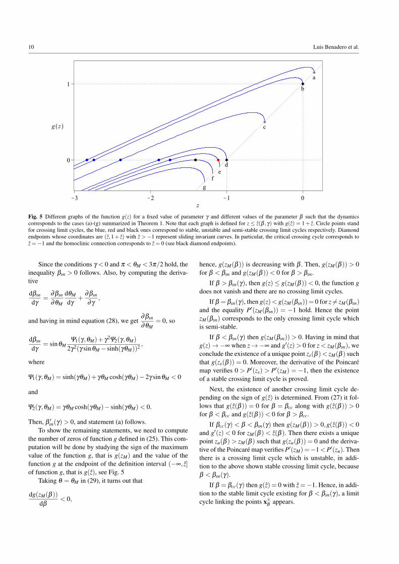
Fig. 5 Different graphs of the function g(z) for a fixed value of parameter γ and different values of the parameter β such that the dynamicscorresponds to the cases (a)-(g) summarized in Theorem 1. Note that each graph is defined for z ≤ z(β ,γ) with g(z) = 1+ z. Circle points standfor crossing limit cycles, the blue, red and black ones correspond to stable, unstable and semi-stable crossing limit cycles respectively. Diamondendpoints whose coordinates are (z,1+ z) with z > −1 represent sliding invariant curves. In particular, the critical crossing cycle corresponds toz =−1 and the homoclinic connection corresponds to z = 0 (see black diamond endpoints).

Since the conditions γ < 0 and π < θM < 3π/2 hold, theinequality βsn > 0 follows. Also, by computing the deriva-tive

dβsn

dγ=

∂βsn

∂θM

dθM

dγ+

∂βsn

∂γ,

and having in mind equation (28), we get∂βsn

∂θM= 0, so

dβsn

dγ= sinθM

Ψ1(γ,θM)+ γ2Ψ2(γ,θM)

2γ2(γ sinθM− sinh(γθM))2 ,

where

Ψ1(γ,θM) = sinh(γθM)+ γθM cosh(γθM)−2γ sinθM < 0

and

Ψ2(γ,θM) = γθM cosh(γθM)− sinh(γθM)< 0.

Then, β ′sn(γ)> 0, and statement (a) follows.To show the remaining statements, we need to compute

the number of zeros of function g defined in (25). This com-putation will be done by studying the sign of the maximumvalue of the function g, that is g(zM) and the value of thefunction g at the endpoint of the definition interval (−∞, z]of function g, that is g(z), see Fig. 5

Taking θ = θM in (29), it turns out that

dg(zM(β ))

dβ< 0,

hence, g(zM(β )) is decreasing with β . Then, g(zM(β )) > 0for β < βsn and g(zM(β ))< 0 for β > βsn.

If β > βsn(γ), then g(z)≤ g(zM(β ))< 0, the function gdoes not vanish and there are no crossing limit cycles.

If β = βsn(γ), then g(z)< g(zM(βsn))= 0 for z 6= zM(βsn)

and the equality P′(zM(βsn)) = −1 hold. Hence the pointzM(βsn) corresponds to the only crossing limit cycle whichis semi-stable.

If β < βsn(γ) then g(zM(βsn)) > 0. Having in mind thatg(z)→−∞ when z→−∞ and g′(z)> 0 for z < zM(βsn), weconclude the existence of a unique point zs(β )< zM(β ) suchthat g(zs(β )) = 0. Moreover, the derivative of the Poincarémap verifies 0 > P′(zs) > P′(zM) = −1, then the existenceof a stable crossing limit cycle is proved.

Next, the existence of another crossing limit cycle de-pending on the sign of g(z) is determined. From (27) it fol-lows that g(z(β )) = 0 for β = βcc along with g(z(β )) > 0for β < βcc and g(z(β ))< 0 for β > βcc.

If βcc(γ) < β < βsn(γ) then g(zM(β )) > 0,g(z(β )) < 0and g′(z) < 0 for zM(β ) < z(β ). Then there exists a uniquepoint zu(β )> zM(β ) such that g(zu(β )) = 0 and the deriva-tive of the Poincaré map verifies P′(zM)=−1<P′(zu). Thenthere is a crossing limit cycle which is unstable, in addi-tion to the above shown stable crossing limit cycle, becauseβ < βsn(γ).

If β = βcc(γ) then g(z) = 0 with z =−1. Hence, in addi-tion to the stable limit cycle existing for β < βsn(γ), a limitcycle linking the points x±B appears.


(a) β < βhc(γ) (b) β = βhc(γ)

(c) βhc(γ)< β < βcc(γ) (d) β = βcc(γ)

(e) βcc(γ)< β < βsn(γ) (f) β = βsn(γ)

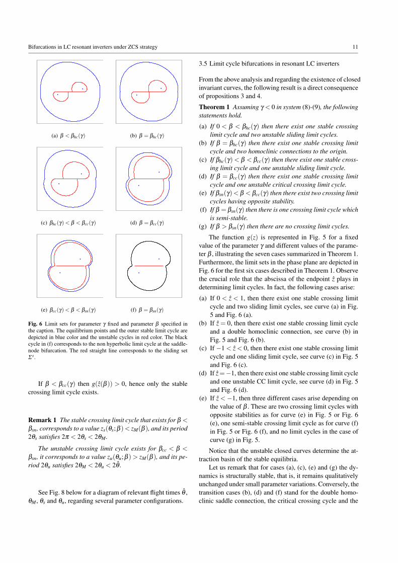
Fig. 6 Limit sets for parameter γ fixed and parameter β specified inthe caption. The equilibrium points and the outer stable limit cycle aredepicted in blue color and the unstable cycles in red color. The blackcycle in (f) corresponds to the non hyperbolic limit cycle at the saddle-node bifurcation. The red straight line corresponds to the sliding setΣ s.

If β < βcc(γ) then g(z(β )) > 0, hence only the stablecrossing limit cycle exists.

Remark 1 The stable crossing limit cycle that exists for β <

βsn, corresponds to a value zs(θs;β )< zM(β ), and its period2θs satisfies 2π < 2θs < 2θM .

The unstable crossing limit cycle exists for βcc < β <

βsn, it corresponds to a value zu(θu;β )> zM(β ), and its pe-riod 2θu satisfies 2θM < 2θu < 2θ .

See Fig. 8 below for a diagram of relevant flight times θ ,θM , θs and θu, regarding several parameter configurations.

3.5 Limit cycle bifurcations in resonant LC inverters

From the above analysis and regarding the existence of closedinvariant curves, the following result is a direct consequenceof propositions 3 and 4.

Theorem 1 Assuming γ < 0 in system (8)-(9), the followingstatements hold.

(a) If 0 < β < βhc(γ) then there exist one stable crossinglimit cycle and two unstable sliding limit cycles.

(b) If β = βhc(γ) then there exist one stable crossing limitcycle and two homoclinic connections to the origin.

(c) If βhc(γ)< β < βcc(γ) then there exist one stable cross-ing limit cycle and one unstable sliding limit cycle.

(d) If β = βcc(γ) then there exist one stable crossing limitcycle and one unstable critical crossing limit cycle.

(e) If βsn(γ)< β < βcc(γ) then there exist two crossing limitcycles having opposite stability.

(f) If β = βsn(γ) then there is one crossing limit cycle whichis semi-stable.

(g) If β > βsn(γ) then there are no crossing limit cycles.

The function g(z) is represented in Fig. 5 for a fixedvalue of the parameter γ and different values of the parame-ter β , illustrating the seven cases summarized in Theorem 1.Furthermore, the limit sets in the phase plane are depicted inFig. 6 for the first six cases described in Theorem 1. Observethe crucial role that the abscissa of the endpoint z plays indetermining limit cycles. In fact, the following cases arise:

(a) If 0 < z < 1, then there exist one stable crossing limitcycle and two sliding limit cycles, see curve (a) in Fig.5 and Fig. 6 (a).

(b) If z = 0, then there exist one stable crossing limit cycleand a double homoclinic connection, see curve (b) inFig. 5 and Fig. 6 (b).

(c) If −1 < z < 0, then there exist one stable crossing limitcycle and one sliding limit cycle, see curve (c) in Fig. 5and Fig. 6 (c).

(d) If z=−1, then there exist one stable crossing limit cycleand one unstable CC limit cycle, see curve (d) in Fig. 5and Fig. 6 (d).

(e) If z <−1, then three different cases arise depending onthe value of β . These are two crossing limit cycles withopposite stabilities as for curve (e) in Fig. 5 or Fig. 6(e), one semi-stable crossing limit cycle as for curve (f)in Fig. 5 or Fig. 6 (f), and no limit cycles in the case ofcurve (g) in Fig. 5.

Notice that the unstable closed curves determine the at-traction basin of the stable equilibria.

Let us remark that for cases (a), (c), (e) and (g) the dy-namics is structurally stable, that is, it remains qualitativelyunchanged under small parameter variations. Conversely, thetransition cases (b), (d) and (f) stand for the double homo-clinic saddle connection, the critical crossing cycle and the


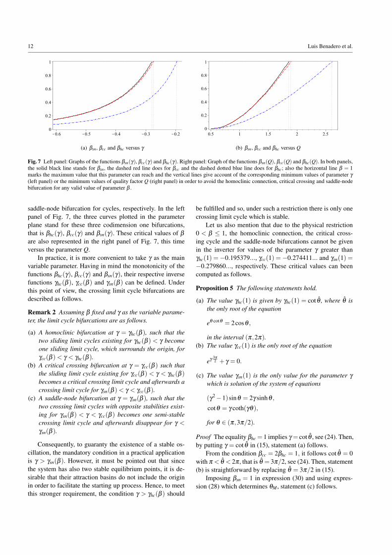
(a) βsn, βcc and βhc versus γ (b) βsn, βcc and βhc versus Q

Fig. 7 Left panel: Graphs of the functions βsn(γ), βcc(γ) and βhc(γ). Right panel: Graph of the functions βsn(Q), βcc(Q) and βhc(Q). In both panels,the solid black line stands for βsn, the dashed red line does for βcc and the dashed dotted blue line does for βhc; also the horizontal line β = 1marks the maximum value that this parameter can reach and the vertical lines give account of the corresponding minimum values of parameter γ

(left panel) or the minimum values of quality factor Q (right panel) in order to avoid the homoclinic connection, critical crossing and saddle-nodebifurcation for any valid value of parameter β .

saddle-node bifurcation for cycles, respectively. In the leftpanel of Fig. 7, the three curves plotted in the parameterplane stand for these three codimension one bifurcations,that is βhc(γ), βcc(γ) and βsn(γ). These critical values of β

are also represented in the right panel of Fig. 7, this timeversus the parameter Q.

In practice, it is more convenient to take γ as the mainvariable parameter. Having in mind the monotonicity of thefunctions βhc(γ), βcc(γ) and βsn(γ), their respective inversefunctions γhc(β ), γcc(β ) and γsn(β ) can be defined. Underthis point of view, the crossing limit cycle bifurcations aredescribed as follows.

Remark 2 Assuming β fixed and γ as the variable parame-ter, the limit cycle bifurcations are as follows.

(a) A homoclinic bifurcation at γ = γhc(β ), such that thetwo sliding limit cycles existing for γhc(β ) < γ becomeone sliding limit cycle, which surrounds the origin, forγcc(β )< γ < γhc(β ).

(b) A critical crossing bifurcation at γ = γcc(β ) such thatthe sliding limit cycle existing for γcc(β ) < γ < γhc(β )

becomes a critical crossing limit cycle and afterwards acrossing limit cycle for γsn(β )< γ < γcc(β ).

(c) A saddle-node bifurcation at γ = γsn(β ), such that thetwo crossing limit cycles with opposite stabilities exist-ing for γsn(β ) < γ < γcc(β ) becomes one semi-stablecrossing limit cycle and afterwards disappear for γ <

γsn(β ).

Consequently, to guaranty the existence of a stable os-cillation, the mandatory condition in a practical applicationis γ > γsn(β ). However, it must be pointed out that sincethe system has also two stable equilibrium points, it is de-sirable that their attraction basins do not include the originin order to facilitate the starting up process. Hence, to meetthis stronger requirement, the condition γ > γhc(β ) should

be fulfilled and so, under such a restriction there is only onecrossing limit cycle which is stable.

Let us also mention that due to the physical restriction0 < β ≤ 1, the homoclinic connection, the critical cross-ing cycle and the saddle-node bifurcations cannot be givenin the inverter for values of the parameter γ greater thanγhc(1) =−0.195379..., γcc(1) =−0.274411... and γsn(1) =−0.279860..., respectively. These critical values can beencomputed as follows.

Proposition 5 The following statements hold.

(a) The value γhc(1) is given by γhc(1) = cot θ , where θ isthe only root of the equation

eθ cotθ = 2cosθ ,

in the interval (π,2π).(b) The value γcc(1) is the only root of the equation

eγ3π2 + γ = 0.

(c) The value γsn(1) is the only value for the parameter γ

which is solution of the system of equations

(γ2−1)sinθ = 2γ sinhθ ,

cotθ = γ coth(γθ),

for θ ∈ (π,3π/2).

Proof The equality βhc = 1 implies γ = cot θ , see (24). Then,by putting γ = cot θ in (15), statement (a) follows.

From the condition βcc = 2βhc = 1, it follows cot θ = 0with π < θ < 2π , that is θ = 3π/2, see (24). Then, statement(b) is straightforward by replacing θ = 3π/2 in (15).

Imposing βsn = 1 in expression (30) and using expres-sion (28) which determines θM , statement (c) follows.


Fig. 8 Plots of the functions θs(γ) in solid blue, θu(γ) in solid red, θ(γ)in dash black and θM(γ) in dash-dotted black versus parameter γ , withparameter β ∈B. Note that θs = π when β = 0 and in the other cases,the four sets of two vertical lines indicate the smooth saddle-node andthe critical crossing bifurcations for cycles at γsn and γcc respectively.

4 Oscillation features regarding applications

This section is addressed to compute the frequency and sizeof the stable crossing limit cycle by considering γ as themain variable parameter. Notice that in the context of ap-plications, the system is expected to behave properly undersome specified load range. In practice a variation in the loadresistor, Ros or Rop, would produce a significant change inthe parameter γ , but minor changes in the parameter β .

According to Remarks 1-2, the stable limit cycle existsfor γsn(β )< γ < 0 with a half-period θs satisfying π < θs <

θM .Once computed θs as the smaller value for θ vanishing

(26), from the time changes used in propositions 1 and 2 wecan compute the period T (or the corresponding frequencyω = 2π/T ) of the stable oscillation in system (1). Since thenormalized time θ in system (8)-(9) is related to the realtime t in system (1)-(2) by the relation θ = ω0νt, we obtainT = 2θs/(νω0). Then, the relative frequency ωr with respectto the natural frequency ω0 is

ωr =ω

ω0=

πν

θs=

π

θs√

1+ γ2=

π

θs

√1− 1

4Q2 .

In order to evaluate the size of the oscillation, let us usethe absolute value of the intersection of the stable crossinglimit cycle with the switching manifold Σ , which will be de-noted as Σ−amplitude, for short aΣ . Then aΣ = P(z(θs)) =

|z(θs)|> 0, and from (17)-(18),

aΣ =P(z(θs))+ |z(θs)|

2= 2βγ

cosh(γθs)− cosθs

(1+ γ2)sinθs.

To illustrate the parameter dependence of these magni-tudes, they will be represented as function of either γ or Q,and β will be chosen within the set

B = {0,1/4,1/2,3/4,1}.

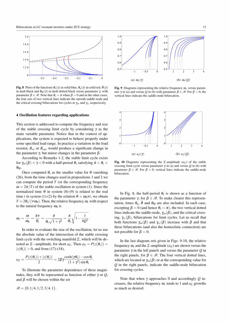
(a) ωr(γ) (b) ωr(Q)

Fig. 9 Diagrams representing the relative frequency ωr versus param-eter γ in (a) and versus Q in (b) with parameter β ∈B. For β > 0, thevertical lines indicate the saddle-node bifurcation.

(a) aΣ (γ) (b) aΣ (Q)

Fig. 10 Diagrams representing the Σ -amplitude (aΣ ) of the stablecrossing limit cycle versus parameter γ in (a) and versus Q in (b) withparameter β ∈ B. For β > 0, vertical lines indicate the saddle-nodebifurcation.

In Fig. 8, the half-period θs is shown as a function ofthe parameter γ , for β ∈B. To make clearer this represen-tation, times θu, θ and θM are also included. In each case,excepting β = 0 (and hence θs = π), the two vertical dottedlines indicate the saddle-node, γsn(β ), and the critical cross-ing, γcc(β ), bifurcations for limit cycles. Let us recall thatboth functions γsn(β ) and γcc(β ) increase with β and thatthese bifurcations (and also the homoclinic connection) arenot possible for β = 0.

In the last diagram sets given in Figs. 9-10, the relativefrequency ωr and the Σ -amplitude (aΣ ) are shown versus theparameter γ in the left panels and versus the parameter Q inthe right panels, for β ∈B. The four vertical dotted lines,which are located at γsn(β ) or at the corresponding value forQ in the right panels, indicate the saddle-node bifurcationfor crossing cycles.

Note that when γ approaches 0 and accordingly Q in-creases, the relative frequency ωr tends to 1 and aΣ growthsas much as desired.


5 Conclusions

Emerging applications of power electronics have recentlymotivated the use of soft switching self oscillating resonantparallel and series converters because their advantages withrespect to their hard switching counterparts. The design andthe stability analysis of these systems are challenging tasks,which are usually performed using different procedures fromcontrol theory, as if they were applied to smooth dynam-ical systems. For instance, averaging, describing functionand Hamel locus methods have been applied, possibly lead-ing to inaccurate predictions about the real dynamics of thenon-smooth system. Moreover, the analysis of the dynam-ical behavior of these systems is conventionally performedcase by case, clearly distinguishing between parallel and se-ries resonant inverters.

In this paper, first, a unified circuit diagram and its equiv-alent non smooth model have been derived allowing to per-form a unified and rigorous mathematical study for bothsystems through the introduction of a continuous parame-ter (called β in this paper), which also takes into accountthe parasitic elements. The extreme cases β = 0 and β = 1correspond to the ideal series and to the ideal parallel im-plementations respectively. Using this generalized model,non smooth bifurcation phenomena in LC resonant paral-lel and series inverters under zero current switching strat-egy are studied. Analytical expressions, for both the limitsets and the bifurcation values of the parameters, have beenfound, thus providing more understanding and quantitativeinformation for real circuits than in previous literature. Thebifurcation scheme explains the coexistence of different at-tractors in these inverters, giving details in both the stateplane and the parameter plane to prevent undesired dynam-ics. Hence, the model and the methods presented in thiswork can help to design LC resonant inverters more effec-tively, which is especially challenging if a global pictureof all the possible dynamics is of concern. Some issues re-garding applications like amplitude and frequency of oscil-lations, that are highly useful in control design, are also de-termined while avoiding, whenever it was possible, numeri-cal procedures.

References

1. Suryawanshi, H.M., Tarnekar, S.G.: Resonant converter in highpower factor, high voltage DC applications. IEE Proc. - Electr.Power Appl. 145, 4, 307-314 (1998)

2. Schwarz, F.C.: An Improved Method of Resonant Current PulseModulation for Power Converters. IEEE Trans. on Ind. Electron.and Control Instrum. 23, 2, 133-141 (1976)

3. Steigerwald, R.L., Ngo, K.D.T.: Full bridge lossless switching con-verter. U.S. Patent 4 864 479 (1989)

4. Samanta, S., Rathore, A.K.: A New Current-Fed CLC Transmit-ter and LC Receiver Topology for Inductive Wireless Power Trans-

fer Application: Analysis, Design, and Experimental Results. IEEETrans. on Transportation Electrification. 1, 4, 357-368 (2015)

5. Fernandes, R.C, de Oliveira, A.A.: Theoretical bifurcation bound-aries for Wireless Power Transfer converters. IEEE 13th Brazil-ian Power Electron. Conf. and 1st Southern Power Electron. Conf.(COBEP/SPEC). 1-4., Fortaleza (2015)

6. Bonache-Samaniego, R., Olalla, C., Martínez-Salamero, L., Mak-simovic, D.: 6.78 MHz self-oscillating parallel resonant converterbased on GaN technology. 2017 IEEE Applied Power Electron.Conf. and Expos. (APEC). 1594-1599, Tampa, FL (2017)

7. Deng, J., Li, S., Hu, S., Mi, C.C., Ma, R.: Design Methodologyof LLC Resonant Converters for Electric Vehicle Battery Chargers.IEEE Trans. on Veh. Technol. 63, 4, 1581-1592 (2014)

8. Baya, B.: Simplified model of resonant inverters for the modelisa-tion of induction heating of billet. IECON 40th Annual Conferenceof the IEEE Ind. Electron. Soc. 3270-3276, Dallas (2014)

9. Schnell, R.W., Zane, R.A., Azcondo, F.J.: HID lamp driver withphase controlled resonant-mode ignition detection and fast transi-tion to LFSW warm-up mode. IEEE 12th Workshop on Control andModel. for Power Electron. (COMPEL). 1-8, Boulder, CO (2010)

10. Erickson, R.W., Maksimovic, D.: Fundamentals of Power Elec-tronics. Lluwer, Springuer (2001)

11. Bonache-Samaniego, R., Olalla, C., Martínez-Salamero, L.: De-sign of self-oscillating resonant converters based on a variablestructure systems approach. IET Power Electron. 57, 1, 111-119(2015)

12. Ehsani, M.: Power conversion using zero current soft switching.U.S. Patent 5 287 261 (1994)

13. Andronov, A.A., Vitt, A., Khaikin, S.E.: Theory of oscillators.Pergamon Press, Oxford (1966)

14. di Bernardo, M., Budd, C.J., Champneys, A.R., Kowalczyk, P.:Piecewise-Smooth Dynamical Systems: Theory and Applications,Appl. Math. Sci. 163, Springer-Verlag London Ltd., London (2008)

15. Filippov, A.F., Arscott, F.M.: Differential Equations with Discon-tinuous Right-Hand Sides. Kluwer Academic, Dordrecht (1988).

16. Kuznetsov, Yu.A., Rinaldi, S., Gragnani, A.: One-Parameter Bi-furcations in Planar Filippov Systems. Int. J. Bifurc. Chaos 13,2157-2188 (2003)

17. Freire, E., Ponce, E., Torres, F.: Canonical discontinuous planarpiecewise linear systems. SIAM J. Appl. Dyn. Syst. 20, 11, 181-211 (2012)

18. Freire, E., Ponce, E., Torres, F.: A general mechanism to gener-ate three limit cycles in planar Filippov systems with two zones.Nonlinear Dynamics 78, 251-263 (2014)

19. Freire, E., Ponce, E., Torres, F.: On the critical crossing cycle bi-furcation in planar Filippov systems. J. Differ. Eq. 259, 7086-7107(2015)

20. Coll, B., Gasull, A., Prohens, R.: Degenerated Hopf bifurcation indiscontinuous planar systems. J. Math. Anal. Appl. 253, 671-690(2001)

21. Han, M., Zhang, W.: On Hopf bifurcation in non-smooth planarsystems. J. Differ. Eq. 248, 2399-2416 (2010)

22. Chen, X., Romanovski, V., Zhang, W.: Degenerate Hopf bifurca-tions in a family of FF-type switching systems J. Math. Anal. Appl.432, 1058-1076 (2015)

23. Chen, X., Llibre, J., Zhang, W.: Averaging approach to cyclicity ofHopf bifurcations in planar linear-quadratic polynomials discontin-uous differential systems. Disc. Cont. Dyn. Syst., 22, 10, 3953-3965(2017)

24. Giannakopoulos, F., Pliete, K.: Planar systems of piecewise lineardifferential equations with a line of discontinuity. Nonlinearity 14,1611-1632 (2001)

Documents

Limit cycle bifurcations in resonant LC power inverters