Life Course Data in Demography and Social Sciences:

Statistical and Data Mining Approaches

Gilbert Ritschard and Michel Oris University of Geneva1

Abstract This paper has essentially a methodological purpose. In a first section,

we shortly explain why demographers have been relatively reluctant to implement the life course paradigm and methods, while the quantitative focus and the concepts of demographic analysis a priori favored such implementation. A real intellectual crisis has been needed before demographers integrated the necessity to face up the challenge of shifting “from structure to process, from macro to micro, from analysis to synthesis, from certainty to uncertainty” (Willekens, 1999, p. 26). This retrospective look also shows impressive progresses to promote a real interdisciplinarity in population studies, knotting the ties between demography and the social sciences. However, we also note that the success of multivariate causal analyses has been so rapid that some pitfalls are not always avoided. In Section 2, we focus on statistical methods for studying transitions. First, readers mind is refreshed about regression like models, and then we consider the issue of population heterogeneity. We show how it could affect results interpretation, and illustrate the interest of robust estimates and of the notion of shared frailty to deal with it. We also present Markovian modeling. Though less popular than regression event history models, Markovian models are specifically well suited for studying successive transitions between states observed at periodic time. In Sections 3, we promote some tools from the developing field of data mining, with special attention on the mining of frequent sequences and induction trees. These highly flexible heuristic tools can, among others, handle trajectories. Hence, they may prove very useful to face the deficit of knowledge on trajectories we observe between standard demographic analysis and causal research.

1 From demographic analysis to life course approach Although demographic analysis has a long history (see Dupâquier and Dupâquier, 1985), the methods still used today have essentially been elaborated between the mid nineteenth and the mid twentieth century in Western societies that felt successively threatened by race degeneration, declining birth rates and ageing. The macro frame was that of the demographic transition, i.e. the evolution from young populations with high 1 Gilbert Ritschard (gilbert.ritschard@themes.unige.ch) is at the Department of Econometrics and Michel Oris (michel.oris@histec.unige.ch) at the Department of Economic History. Both belong also to the Laboratory of Demography and Family Studies and have benefited, for this research, from an help of the Swiss National Science Foundation, projects 1114-68113 and 100012-105478.

2

fertility and high (especially infant and child) mortality to ageing populations with net reproduction below the threshold of generations’ renewal and a tremendous increase in life expectancy at birth.

From a methodological point of view, a starting point in demographic analysis has been the mortality table. It implies a dynamic perception of population with entrances (births or in-migrations) and exits (deaths or out-migrations), and the idea that other events (like migration) can censor a given risk (like mortality). It rapidly constrained the conceptual distinction between a generation – i.e. those who are born in the same year or period – and a cohort – i.e. those who are experiencing an event (marriage for example) in the same year or period. The mortality table also resulted not only in an average age at death but in a distribution of the risk along the life course, providing a survival curve. Finally, the immediate comparison of these curves among sexes, and even more among matrimonial statuses, revealed selection processes, like those supporting the over-mortality of singles compared to married people. Heterogeneity and differential frailty were not ignored. After the generalization of mortality analysis (from mortality- to life-tables), certainly no scientific discipline was better prepared for the life course methods than demography. Nevertheless, the paradigms clearly diverged.

First, dealing with structures and flows, demography has been a science of reconstruction and description of patterns and behaviors, through a well-established quantitative methodology, and the conviction that higher the number of observations, more accurate - and possibly useful – were the results (see, as a typical example, Vallin 2001). Demography was a science of the masses, growing or stagnating, young or old, but not of the individuals!

Second, the engagement of generations of scholars was largely motivated by the central character of population issues and the location of demography at a crossroad between economy, sociology, epidemiological studies, territorial analysis, political sciences and, more recently, cultural and gender approaches. However, research and collaborations were in reality highly segmented, with a clear tendency to specialization on a geographical and/or thematic basis (typically mortality, fertility, marriage and family formation or dissolution, migrations, structures, prospective). Among many others, the last edition of the excellent Encyclopedia of Population (Demeny and McNicoll, 2003) illustrates that propensity. Such segmentation was clearly inscribed in the methods. In the estimations of mortality, mobility was statistically treated as a censor but explicitly presented as a bias for a “pure” analysis of mortality. Clearly, the approach consisted in studying a demographic behavior as independently as possible from the other ones, without systemic perspectives.

Third, the demographic evolution made apparent the limits of the established methodology. Both mortality- and life-tables can be calculated longitudinally, based on the observation of generations, or on cross-sectional data, i.e. the observation of deaths by age classes at a given time point – mixing thus generations with different history together. For the simplest table, that of mortality, since expectation of life at birth now exceeds 80, the longitudinal approach implies a population reconstruction from at least the 1920s, what is quite difficult, especially if we do not accept the hypothesis of a null effect of migration. Inversely, all the statistical offices of the developed countries collect the data for the calculation of cross-sectional measures since a long time. However, can we accept the underlying hypothesis of continuity while the duration of life wins one year each three to four years and while we know that the – generational – age

3

distribution of those gains has drastically changed during the last decades? Similarly, while in the context of the so-called “second demographic transition” there are so many changes in the fertility calendar, do we have to constrain ourselves to the observation of those generations who have finished their fertile life and renounce to study the present with other indicators than those of the moment? What is today the rationale of detailing the access to marriage while cohabitation is rising? How record an informal event like entrance in cohabitation? Both data collection and analytical tools have been challenged by recent changes in demographic behaviors and family dynamics (for a more in-depth discussion of those issues, see Caselli, Vallin and Wunsch, 2001).

A real intellectual crisis resulted from the hesitation about the status of demography within the social sciences, as well as from the frustration against segmentation and the deficiency of old methods. Also grew the conscience that description, especially some quantification with a pretension of objectivity, hid and diffused ideological visions about “good” or “optimal” populations (Greenhalgh 1996; van der Kaa 1996; Véron, 1993; Szreter, 1993; Hogdson 1988 and 1991; and many others).

Among the many reactions, revisions and re-examinations, new approaches and new methods rapidly emerged. No significant use of the life course statistical tools can be observed before the mid 1980s, while for example Cox foundling paper is dated 1972. When they finally have been integrated by demographers, the new methods found many use. Probably the most obvious progress they supported was to replace demography in its family setting. Something that could seem very strange, but perfectly illustrates this assertion, is indeed the discovery, precisely in the 1980s, of an almost complete absence of dialogue between demography and family sociology. While family is the place where most of the demographic behaviors take place and, to some extent, are decided, “few textbooks on population contain a chapter devoted to the demography of the family. Where such chapter does exist, it is generally shorter and more superficial than those that deal with fertility, mortality, nuptiality, and migration, or with the dynamics of age structure” (Höhn, 1992, p. 3). In 1982, the International Union for the Scientific Study of Population created an ad hoc committee to develop its study, but still in 1992 the animators of this group saw family demography as “a recent and relatively underdeveloped branch of population studies” (Berquo and Xenos, 1992, p. 8).

Its development has been extraordinary in the last years. Francesco Billari chapter in this volume, provides a nice illustration of such change, which is part of a shift from macro to micro, from an emphasis on macro-economic evolutions as the essential determinant of demographic “answers”, to a multi-causal - multivariate - approach of behaviors, a shift also from average results to a more detailed study of distributions. In a quantitative discipline, major evolutions necessarily imply to take up technical challenges. “The traditional demographic analysis of such events as births, marriages, divorces, deaths, and migration, has the advantage that numbers of these events can be related to individuals in the same age group and can, therefore, be measured more easily and included in models. The inclusion of other family members in such analyses causes difficulties because they will generally differ in age and sex, and complications are also introduced because they do not generally live together continuously” (Höhn, 1992, p. 3).

Although several attempts have been done to construct a “household demography” (Van Imhoff et al., 1995), the life course paradigm and its methodological individualism clearly imposed themselves. Offering both concepts and statistical methods, it represents a shift toward micro analysis of individual data and causal research that not

4

only deeply renews the discipline, but also provides the vocabulary for a new inter-disciplinarity, first within the social sciences, then beyond (Blossfelfd and Rohwer 2002; Dykstra and van Wissen, 1999). A first substantial gain has been the study of multiple events, marriage and first birth, or moving and starting a new job for instance, a kind of investigation that also raise the issue of event sequencing and interactions that is typically treated with event history analysis. If people have several careers that they must make compatible, their life transitions also reflect socio-economic constraints, cultural norms (about the “proper” age, sex or behavior), as well as compromises between several individual aspirations within or beyond the domestic unit. Through researches in this huge area, family demography made for sure tremendous progress during the last 20 years.

However, the shift has been so sudden that globally the complexity of causalities remains too often under-estimated (see especially Courgeau and Lelièvre, 1993; Blossfeld and Rowher, 2002; Bocquier, 1996; Alter, 1998; Billari here), as well as several technical traps. The problem is essentially that when studying a population of individuals observed along the time, since each life, product of complex and multiple interactions, is as a matter of fact unique. Hence, interpreting and generalizing from samples requires several cautions. In the next section, we remind the main event history regression models and discuss the question of heterogeneity. We cannot consider that the elaboration of indicators at an individual level about household, family and community contexts is enough to deal with the more and more raised issue of “linked” or “interdependent” lives (Hagestad, 2003). We show the interest of robust estimates and shared frailty in that perspective. In the same section, we also present the Markovian models that are particularly useful for the study of transitions within a set of states (matrimonial or social status, for example) periodically observed. In the interdisciplinary perspective that is the one of life course, we consider important to go beyond the simple transitions typically studied in demography (from single to married, from a first to a possible second child, from life to death, and so on) and to investigate how, from a starting position, a destination is selected among several possible. While family dynamics and life courses are more and more open, such investigations are essential to deal with the characterization of transitions as “normal” or “non-normal” without falling again in the trap of ideological reading (see, for example, the discussion in Oris and Poulain, 2003, about the stigmatization of early leaving home).

Indeed, we assess more globally that between aggregate descriptions and causal analysis there is a deficit of research on trajectories. Regression models attempt to quantify how a factor, measured by an indicator, affects a risk. Such results tell us nothing, however, about the calendar and no more about the alternatives to this risk in life courses. It is essential to look carefully at transitions in trajectories to properly target a causal analysis, and this step is clearly too often superficial, if not absent. Several methods, recently developed or recently made available in statistical packages, offer opportunities to fill this gap. Among them, we discuss in Section 3 data mining tools, especially mining event sequential association rules and induction trees that seem to us the more promising for life course data analysis.

2 Statistical modeling of life events Life courses data are longitudinal in their essence. Here, we focus on events, an event being the change of state of some discrete variable, e.g. the marital status, the number of

5

children, the job, the place of residence. Such data are collected in mainly two ways: as a collection of time stamped events or as state sequences. In the former case, each individual is described by a collection of time stamped events, i.e. the realization of each event of interest (e.g. being married, birth of a child, end of job, moving) is mentioned together with the time at which it occurred. In the second case, the life events of each individual are represented by the sequence of states of the variables of interest. Panel data are special case of state sequences where the states are observed at periodic time. The first kind of data is typically analyzed with event history regression methods, while methods for state sequence analysis like Markov transition models are best suited for the latter. We briefly discuss hereafter the scope and limits of these approaches.

2.1 Event history regression models When we have time stamped events, the question of interest is the duration of the spell between two successive events, or somewhat equivalently the hazard rate h(t) for the next event to occur precisely after a duration t, i.e. the conditional probability for the event to occur at t knowing that it did not occur before t. Longitudinal regression models focus on this aspect. They express either the duration or the hazard rate as a function of covariates. It is worth mentioning that these models are also known as survival models, especially in area like biomedicine and engineering where the event of concern is just death or breakdown.

There are continuous time models and discrete time forms. With continuous time, the main formulations (see Blossfeld et al., 1989; Courgeau and Lelièvre, 1993) are as a duration model or as a proportional hazard model. Duration models consider ln(T), the logarithm of the time to the event, as a linear function of the explanatory factors. Proportional hazard models suppose that the ratio between the hazard for a given profile (in terms of the covariates) and that for a reference baseline profile remains constant over time and expresses the logarithm of this ratio (or proportion) as a linear function of the covariates.

Duration models, also known as accelerated failure time models, assume usually an exponential, Weibull, log-normal, log-logistic or gamma distribution for the duration T. The proportional hazard model is compatible with for instance, exponential, Weibull and Gompertz duration distributions. It includes also the perhaps most widely used Cox (1972) semi-parametric model that requires no assumptions on the form of the duration distribution. Most statistical packages (SAS, S-Plus, Stata, R, TDA, ...) provide procedures for estimating such models. At least until version 13, SPSS, however, offers only support for the Cox model.

Discrete time models (see Allison, 1982; Yamaguchi, 1991) include the proportional hazard-odd model, also due to Cox (1972), the discrete proportional hazard model (Aranza-Ordaz, 1983) and the log-rate model (Holford, 1980). In the former, it is not just the hazard ratio, but the ratio of the odds of the hazards that is supposed constant and having a logarithm depending linearly on the covariates. The discrete proportional hazard model expresses the log minus log of the complementary hazard as a linear function of the covariates. The log-rate model on its side, expresses the log-hazard in terms of proper and interaction effects of categorical variables and also possibly of their interactions with duration.

6

For the estimation of the proportional hazard-odd model, some assumptions are usually required upon the baseline hazard-odd. Letting t0β be the baseline log-hazard-odd after a duration t, the most common assumptions are that it remains constant with t, is linear in t (Gompertz) or is linear in ln(t) (Weibull). With these assumptions, a proportional hazard-odd model can, if we organize the data in a person-period form, simply be estimated as a logistic regression. Hence, it can be estimated by any software that proposes logistic regression. Likewise, a log-rate model can be estimated with any log-linear model procedure that allows for weighted cell frequencies. Indeed, the log-rate model is a log-linear model of the weighted number of events occurring in a time interval, the weight being the inverse of the population at risk in this interval. The fitting of a discrete proportional hazard model requires the perhaps less frequently implemented procedures for binary regression with a complementary log-log link.

A common issue with the time to event models is the handling of censored data. Censored data occur when the observed start (left) and/or end (right) time of a spell are not its actual start and end time. For instance, if we observe job duration, some jobs may not be terminated at the time of the survey and are hence right censored. Though no event is recorded at the end of the right censored spells, these cases are taken into account by entering the population at risk for job length lower or equal to the observed duration.

Another issue is the handling of time varying covariates. The solution is quite straightforward in the discrete time setting that works on person-time data. For the continuous case, there are two major solutions: an ad-hoc extension of the Cox model that allows for discrete time varying covariate and the episode-splitting approach. (See for instance Blossfeld and Rowher, 2002, for details.) Time varying covariates offer a way to test and relax the somehow strong proportionality assumption required by most hazard rate models. Indeed, this assumption implies the time independency of the ratio of hazards of any two individuals, which clearly does not hold when the ratio depends on a time varying variable. It is common practice to check the significance of the interaction of a supposed time-independent variable with t or ln(t). A significant interaction would provide evidence again time invariance. See Therneau and Grambsch, (2000) for other tests of proportional hazards and more advanced developments of the Cox model.

This event history modeling, especially the Cox proportional hazard and the Cox discrete time proportional hazard odd models, has become popular among demographers. Together with other social science scientists, historical demographers have to face issues like competing events (multiple destinations), repeatable events and interacting events. The first two can easily be handled with a software like TDA (Rohwer and Pötter, 2002) that supports episodes defined by 4 parameters, namely the origin state, the start time, the destination state and the end time. The interaction between events, marriage end and first child for instance needs a simultaneous equation approach that has been investigated for instance by Lillard (1993) and which is discussed more in-depth in Billari’s contribution to this volume.

2.1.1 Shared heterogeneity and multi-level modeling. A further issue of importance, shared heterogeneity, has to do with the sampling nature of the data. These are often clustered, i.e. the individual data come from a selection of groups, parishes or families for example. In such cases, members of a same group share

7

a same contextual framework and it is then of primary importance to distinguish effects that hold at the group level from those that work at the individual level. A very concrete example is the study of orphans survival after father death, ran by Beekink et al. (1999) for a nineteenth century Dutch provincial town. In the event-history file, initially each orphan was considered as a single individual while there were not individuals but groups of siblings that entered in the population at risk because of a shared event – dad death – and supported this experience while sharing the same household context. Taking into account the interrelatedness of the observations changed the results! Along the same line, both in contemporary and historical demography the issue of the death clustering at the family level is a growing concern (Alter et al., 2001). All those studies extend the original discussion of “the impact of heterogeneity in individual frailty on the dynamics of mortality” by Vaupel et al. (1979).

To explain this aspect, let us consider the case of a simple linear regression of the number of children on the education level in the presence of three clusters like those depicted in Figure 1 where the clusters are, let us say, three villages. A simple regression on the whole data set leads to a line with a positive slope, indicating that the number of children increases with education. This effect clearly holds at the aggregated village level, i.e. the higher the average education level in a village, the higher the average number of children. This aggregated effect results despite the regression is fitted on individual data. A separate regression on each cluster exhibits a negative slope in each of the three villages, indicating a negative effect of education on the number of children at the individual level. Indeed similar misleading results may appear when event history regressions are fitted on clustered data as illustrated by the examples discussed by Beekink et al. (1999) and Alter et al. (2001). What are the solutions?

y = 3.2 + 0.2 x

y = 6.2 - 0.8 x

y = 15.6 - 0.8 x

y = 12.5 - 0.8 x

0

1

2

3

4

5

6

7

8

9

1 3 5 7 9 11 13 15

Education

Chi

ldre

n

Figure 1: Multi-level: A simple example with 3 clusters

Table 1 summarizes alternative formulations that can be adopted when we are in

presence of G groups. For the sake of simplicity we consider here regression models with c covariates, generalization to more complex models like event history models

8

being straightforward. Model m1 will capture effects at the group level. In models m2 to m4, differences between groups are introduced by means of additional parameters, an approach that is suitable as long as G is not too large. Model m2 fits separate models on each clusters, while in m3, the regressions are only seemingly independent, since the variance of the error term is supposed to be the same in each group. Model m4 corresponds to the well known case where, for each group, a specific effect is introduced as a dummy variable. For a large number of groups, random effects models2 m5 and m6 are best suited. In these models, the regression coefficients are allowed to vary randomly from one group to another. In the shared frailty formulation, only the constant is random, while the other coefficients remain the same for all groups. The main advantage of these random effect formulations is that their number of parameters is, as can be shown from the last column, independent of the number of clusters. Random effect models m5 and m6 may, therefore, have a much lower number of parameters than models m2 to m4 when G is large.

Table 1: Alternative linear models in presence of G clusters g

model constant effect of

covariate variance of error term

number of parameters

m1 average model same same same 1+c+1

m2 independent group specific group specific group specific G(1+c+1) m3 seemingly indep. group specific group specific same G(1+c)+1 m4 dummies group specific same same G+c+1

m5 random effects random across groups

random across groups

same 2(1+c)+1

m6 shared frailty random across groups

same same 2+c+1

Even if we are interested in the aggregated effect, estimating them with individual

data, as with model m1 for example requires some caution. Indeed, the standard errors of the aggregated effects are derived from individual residuals which may either over- or underestimate the between group discrepancy. For instance, in our example of Figure 1, leaving out in turn each of the three groups leads to great variations in the slope that would be underestimated by the classical standard error. This aspect has been investigated among others by Kish and Frankel (1974) and, for the Cox model for instance by Lin and Wei (1989). In such settings, it is good practice to use robust estimates of the variance of the regression coefficients. Such robust estimates are usually obtained as grouped jackknife estimates, i.e. by measuring the discrepancy of estimates obtained by leaving out successively each of the G clusters, and can be expressed as sandwich estimates (see for instance Therneau and Grambsch, 2000, p. 170–173).

2 Random effects models are also known as multilevel, hierarchical or mixed-effects models.

9

Facilities for dealing with clusters are offered by several statistical systems, Stata 8, S-Plus 6.2 and R 2.0 for instance. All the three mentioned programs propose options to get robust standard errors. They permit also the introduction of a shared frailty in parametric hazard rate and Cox models. Complete random effects are only available with discrete models that can be fitted with logistic regression procedures. Indeed, logistic models are special cases of Generalized Linear Models (GLM).3 Hence, multilevel logistic regression is available whenever multilevel GLM is implemented. Barber et al. (2000) for instance show how to estimate a model with several random effects with the HLM (Bryk et al., 1996) and MLN (Goldstein et al., 1998) programs.

2.1.2 Illustration. To illustrate the scope of robust standard errors and shared frailty we consider a data set of 5351 migrants collected from the 19th century population registers of the Belgian commune of Sart (see Alter and Oris, 2000; Alter et al., 2001, for a detailed description). This data set provides, among others, information about the emigration date, the destination and the date of return after emigration. Table 2 shows results of the fit of a continuous time Cox model. The hazard modeled is that of return after a time between 0 and 5 years, no return or return after 5 years being censored. We fitted a basic model, i.e. without the cluster or frailty options, the same model but requesting robust standard errors for the coefficients, and the model with a gamma γ(1/θ,1/θ) distributed frailty term shared by members of a same family.4

The hazard ratios reported are just the exponential of the coefficients. They indicate the hazard ratio for two profiles that differ by one unit of the corresponding variable. For the frailty model, this interpretation holds assuming the two profiles have a same frailty. For instance, according to the basic model, the chances to return for a single are about one and a half times the chances to return for a non single. Likewise, the probability to return is for a man about 3/4 of that for a woman. We checked on the basic model that none of the time-covariate interactions is significant, which comforts the proportionality assumption.

The coefficients are indeed the same for the basic and robust standard errors models. The significance of the coefficients differs however, as can be seen from the p-values. To be born in the Ardennes is significant at the 5% level when we do not care about the cluster effect, while it is clearly not when we control for it. This indicates that the seemingly significant birth place effect does not work at the family aggregated level. Likewise, we may notice that, though the effect of the household economic ratio is

3 GLM models (McCullagh and Nelder, 1989) cover a large number of parametric models. They assume a distribution of the natural exponential family for the dependent variable and are, in their simpler form, simply characterized by a link function that describes how the mean of the dependent variable is linked to the linear form of the explanatory variables. For example, we get the classical linear model with a Gaussian distribution and the identity link, the logistic model with a Bernoulli distribution and the logit link, and the log-linear model with a Poisson distribution and the log link. 4 The estimations were obtained with S-plus 6.2. We suspect a bug in Stata 8 that was not able to converge within 24 hours for the frailty model while S-Plus provided the results within 2 minutes.

Formally, the estimated hazard model is ),++= 11 ppgp xxthxxth ββν LL exp()(),,,( 01 where h0(t) is the baseline hazard function and gν the shared frailty term. We estimated this model assuming a gamma γ(1/θ,1/θ) distribution for the frailty term gν , for which we have 1)E( =gν and θ)Var( =gν .

10

significant among families, its significance is not as clear as we would expect from the basic model.

Table 2: Cox model for Return within 5 years after emigration, Sart 1812-1900, n=5351

coefficient hazard ratio p-value in % basic frailty basic Frailty basic robust frailty Economic ratio 1.02 0.30 2.76 1.35 0.2 3.8 45.0 Man -0.28 -0.18 0.76 0.83 0.1 0.2 5.6 Single 0.40 0.52 1.49 1.68 1.2 1.2 0.3 Born in Ardennes 0.25 0.17 1.29 1.18 4.1 15.0 28.0 Age when Leaving 0.01 0.00 1.01 1.00 12.0 17.0 62.0 To Ardennes destination reference category To rural -0.32 -0.60 0.73 0.55 5.7 14.0 0.2 To urban/indust. -0.07 -0.23 0.93 0.79 50.0 68.0 6.8 To other -1.25 -1.25 0.29 0.29 0.0 0.0 0.0 Head or spouse of parenthood reference category Child of head 0.02 -0.25 1.02 0.78 89.0 90.0 19.0 Other parenthood 0.12 -0.27 1.13 0.76 54.0 56.0 26.0 No parenthood -0.50 -0.54 0.61 0.58 6.7 7.3 9.0 Standard deviation θ of family effect 1.75 0.0

Let us now look at the results with a family shared frailty. First, we may notice the

highly significant variance of the random term, which clearly indicates a between families discrepancy. Two variables that looked significant become non significant, namely the gender (man) and the economic ratio. This is not surprising for the latter, which is a typical family contextual factor shared by members of a same family. Gender, on the other hand, is clearly an individual characteristic. Its lack of significance in the frailty model seems to indicate that the effect is not systematic within the families. Its overall significance follows probably from differences among male and female singles. A reverse phenomenon is observed for the rural destination effect that becomes significantly different from the reference Ardennes in the frailty model.

2.2 Markov transition models In the presence of state sequences in panel data form, a natural question is what are the transition probabilities from the states at time t−1 to the possible states at time t, and how are these probabilities affected by individual histories or contextual characteristics. Homogenous Markov models assume that these probabilities are independent of the time t. In first order models, the transitions are supposed to depend only upon the state at t−1, which means that the first lag summarizes the whole history of states at t−1 and before. Models of higher order k consider that the transitions depend on k lags, i.e. on the states at t−k,...,t−1. Thus, basic Markov models state that the transition probabilities remain constant over time and depend on a limited, usually small, set of previous states.

11

Markov models of order k generate, when we are in presence of s states, sk transition distributions, i.e. a huge number of probabilities. They may be approximated by Mixture Transition Distribution (MTD) models (Raftery and Tavaré, 1994; Berchtold, 2001; Berchtold and Raftery, 2002) that involve a much lower number of parameters, which renders the models easier to interpret.

Other extensions of the Markov model include the Hidden Markov Model (HMM) (see Rabiner, 1989; MacDonald and Zucchini, 1997) in which the successive states of the observed variable are only indirectly linked through an unobserved Markov chain and the Double Chain Markov Model (DCMM) (Paliwal, 1993; Berchtold, 1999, 2002) which states that the observed states are outcomes of a Markov process randomly selected by a Hidden process. The use of Hidden processes is a way to relax the usually strong homogeneity assumption. For example, when studying social mobility with data covering a whole century, it is hardly defendable to assume that the same process works during the whole period (Lynch 1998, especially p. 96).

Despite their interest, there has been only a limited use of Markov models, especially of non-homogenous ones, by historians and demographers. A search on “Markov” within the famous Population Index data base5 results in only 28 hits among thousands of references. Moreover, most of those 28 hits refer to working papers or highly focused articles (with an emphasis on the study of multistate population dynamics). The main reason of such a limited use is that standard statistical packages offer only limited facilities to fit such models. The available tools require a heavy coding task that discourages most potential users. We can expect, however, that Markov modeling will become much more popular with the recent release of March 2 (Berchtold and Berchtold, 2004). This software offers a friendly way to estimate Markov models without writing down any line of code.

2.2.1 Illustration. To illustrate the nature of knowledge we can expect from such an analysis, we consider here the Blossfeld and Rowher (2002) sample of 600 job episodes extracted from the German Life History Study. The episodes have been classified into 3 job length categories: (1) ≤ 3 years, (2) > 3 and ≤ 10 years, (3) more than 10 years, and the data reorganized into 162 individual sequences of 2 to 9 job episodes, dropping the cases with a single episode. The question considered is how the present episode length depends upon those of the preceding jobs. Notice that the job lengths sequences considered here are not panel data, which demonstrates that Markovian model are not restricted to panel data. In this setting, the subscript t refers simply to the position in the sequence rather to a specific time period.

The first order and second order homogenous transition matrices are given in Table 3. The same table gives also the distribution of the independence model in which the transition probabilities stay the same whatever the previous job length. Let us just briefly illustrate how these tables should be read. The independence distribution tells us that the overall probability for a new job to be a short one is 50% while this probability is 35% for a medium job and 15% for a long job. The first order matrix indicates that the probability that a new job started after a short one has 57% chances to be again a short job. This probability falls to 43% after a job of medium length and to 20% after a 5 http://popindex.princeton.edu/

12

long job. From the second order matrix, it follows for instance that this same probability is 55% when the preceding short job was itself preceded by a short one, 60% when the preceding short job followed a medium job and 100% when the preceding short job followed a long job. The last column in the tables gives the half length of a conservative 95% confidence interval for the probabilities in the concerned row. Hence, probabilities smaller than this half length should be considered as non significant.

Table 3: First and second order homogenous Markov matrices

job length at t half conf.

t−1 1 2 3 interval1 .57 .30 .13 .10 2 .43 .42 .15 .13 3 .20 .53 .27 .29

Indep .50 .35 .15 .07

job length at t half

conf. t−2 t−1 1 2 3 interval1 1 .55 .30 .15 .11 2 1 .60 .30 .10 .20 3 1 1 0 0 .65 1 2 .37 .45 .18 .18 2 2 .50 .41 .09 .20 3 2 .45 .33 .22 .38 1 3 .33 .17 .50 .46 2 3 0 .87 .13 .40 3 3 1 0 0 1

13

Table 4: Two state hidden Markov model

Hidden state at t half conf.

t−1 1 2 interval 1 .78 .22 .12 2 .53 .47 .19

initial .56 .44 .11

Hidden job length half conf.

state 1 2 3 interval 1 .75 .23 .02 .12 2 .05 .58 .37 .18

A glance at these tables leads to the following remarks. The first order matrix

exhibits some differences in the transition probabilities after a short (1), medium (2) or long (3) job. After a first job, the probability to start a short job is significantly higher than to start a medium or long job, while this is not the case after a medium or long job. The second order matrix does not provide evidence on the impact of the lag 2 job length. The main differences concern the transition probabilities after long jobs (3), which are mostly not statistically significant due to the low number of cases concerned. This was confirmed by fitting a MTD model for which we obtained a weight of 1 for the first lag and, hence, 0 for the second lag.

For relaxing the homogeneity assumption, we consider a HMM model with a two hidden state process. Fitting this model we get the distribution of the initial state of the hidden variable, the transition matrix of the hidden process and the distributions of the transition to the job length categories associated to each of the two hidden states. These results are given in Table 4. In addition we get estimates (not shown here) of the most likely sequence of hidden states associated to each observed sequence. Looking at the cross tabulation of these estimated hidden states with the observed job length

observed

hidden 1 2 3 1 118 19 0 2 0 65 35

we see that the first hidden state is mainly associated to short jobs and the second hidden state to medium and long jobs. This may suggest considering only two types of jobs: equal or less than 3 years, and more than 3 years.

14

Table 5: Global model goodness-of-fit statistics

pseudo Model m p −2LogLik Chi2 df sig BIC AIC R2 Indep 2 472.8 0 0 - 483.7 476.8 0 Hom. Order 1 6 462.6 10.2 4 .04 495.4 474.6 .022 Hom. Order 2 13 460.6 12.2 11 .35 531.7 486.6 .026 HMM 2 States 7 468.6 4.2 5 .52 506.9 482.6 .009 number of sequences: 107, usable n = 237

Table 5 summarizes goodness-of-fit statistics for our fitted models and, for the sake of comparison of the independence model. The shown statistics are the number of independent parameters p, the deviance measured as minus twice the log-likelihood6 (−2LogLik), the likelihood ratio Chi-Square statistics that measures the improvement in −2LogLik over independence, its associated degrees of freedom and its significance level, the pseudo R2 that gives the relative improvement in −2LogLik and the AIC and BIC information criteria.7 These figures show that the fitted models do not make much better than the independence model. We get the smallest −2LogLik value for the 2nd order homogenous model, but at the cost of 11 additional independent parameters. The 1st order homogenous model is the only one that significantly improves the −2LogLik of the independence model. It is also slightly better in terms of the AIC. No model outperforms the independence model in terms of the BIC however. These relatively bad results are largely attributable here to the insufficient number of data considered. This stresses a limitation of this Markov modeling approach, namely the complexity of the models in terms of number of estimated parameters that requires a very large number of data.

3 Mining longitudinal life course data Despite the last decade great boost in the use of data mining tools for the knowledge

discovery from data (KDD) in fields ranging from genetics to finance, from marketing to medical diagnosing, from text analysis to image or speech recognition, such approaches have received only little attention for extracting interesting knowledge from longitudinal data describing life courses. An important exception is Blockeel et al. (2001) who showed how mining frequent itemsets may be used to detect temporal changes in event sequences frequency from the Austrian FFS data. In Billari et al. (2000), three of the same authors also experienced an induction tree approach for exploring differences in Austrian and Italian life event sequences. We initiated ourselves (Oris et al., 2003) social mobility analysis with induction trees.

6 The deviance -2LogLik may be seen as the distance between the predictions generated by the model and the observed counts. Hence it is a measure of global fit. However, it cannot be used here to test the fit since we do not know its distribution. 7 The AIC and BIC criteria are penalized forms of the –2LogLik that take account of the complexity, i.e. the number of estimated parameters. Among the two, the BIC is usually prefered since the AIC is known to insufficiently penalize complexity. The model with the minimal BIC offers the best compromise between fit and complexity.

15

Data mining is mainly concerned with the characterization of interesting pattern, either per se (unsupervised learning) or for a classification or prediction purpose (supervised learning). Unlike the statistical modeling approach, it makes no assumptions about an underlying process generating the data and proceeds mainly heuristically.

Beside their non-parametric or assumption free characteristic, data mining methods present also the advantage for our social demographic framework to be able to handle sequences of the various family, education, work, health, emotional and other personal events that define a life course. They seem in that regard promising tools for gaining knowledge about life trajectories and should thus usefully complement the previously discussed statistical methods. Event history models, for example, focus on the risk of a given transition, but do not provide insights on trajectories. Markov models, on the other hand, attempt to characterize the stochastic process that drives successive transitions between states. They provide in that sense some synthetic information about trajectories. However, only trajectories between states of a generally unique variable, social or civil status for example, can be investigated this way. Markov models, even those allowing for covariates, can hardly handle together the various life events. Furthermore, Markov models remain quite rigid by assuming that the transition probabilities do not depend upon the present time but only on a small limited number (the order of the Model) of previous states. From a substantial standpoint, the hereafter discussed sequence mining approach is best suited to discover among the many possible trajectories, for example from the diversity of formations to the diversity of working lives, those that are typical of real life courses of real persons and by contrast those that are atypical.

Since data mining methods are mainly assumption free, exploring trajectories with them may answer to the criticisms of the French sociologist Pierre Bourdieu about the “biographical delusion” (1986). Bourdieu, in fact, denounced the concept of “life cycle”, and its emphasis on norms, norms supposed to lend to “normal” trajectories. With the assumption free mining of longitudinal data, we precisely pass the boarder between the “causality” or “data modeling culture” and what Breiman (2001) calls the “algorithmic culture” (see also the discussion in Billari’s article in this volume).

In the rest of this section, we shortly describe the mining of sequential rules and the induction tree approach, focusing on the nature of knowledge we may expect from such tools. For a more general introduction to data mining, see for instance Hand et al. (2001) or Han and Kamber (2001). These books cover many more methods. The two discussed here are however, in our mind, the two more promising ones for longitudinal data.

3.1 Mining event sequential association rules Each life course can be seen as a sequence of life events: birth, important disease, recovering from disease, starting school, ending school, first job, first union, leaving home, first child, death of father, marriage, ... Mining sequential association rules aims at determining the most typical sequences or subsequences together with their frequencies, and at deriving association rules like, for example, having experienced the subsequence first job, first union, first child, is most likely to be followed by a sequence marriage, second child. By contrast, indeed, mining frequent sequences and rules also reveals atypical life courses. Note that event sequences differ from state sequences as

16

considered by Markov models or optimal matching. Nevertheless, sequence mining could as well be applied to state sequences.

Technically, the mining of frequent event sequences and sequential association rules is a special case of the mining of frequent itemsets and association rules. In data mining, an association rule is just a rule that says that if A occurs then B is very likely to occur too. The basic tuning parameters of the mining process are the support and the confidence thresholds. The support is the minimal frequency in the data base for an itemset to be selected, while the confidence of the rule is the probability that the consequence occurs when the premise is observed. These basic selection criteria are complemented by other additional interestingness measures, like for example the proportion of the rule counter examples. Most algorithms for seeking frequent itemsets and rules are variants of the well known Apriori algorithm (Agrawal and Srikant, 1994; Mannilia et al., 1994). A typical application consists in finding the items that are more often ordered together by customers. Sequences that we consider here differ from general itemsets in that order matters. Multiple algorithms adapted for sequences have been proposed since the pioneering contributions by Agrawal and Srikant (1995) and Mannila et al. (1997).

3.1.1 Illustration. We have not yet ourselves experienced a sequential rule mining analysis on demographic data. For the sake of illustration, we shortly report here the analysis carried out by Blockeel et al. (2001). The data considered originated from the 1995 Austrian Fertility and Family Survey (FFS). The events analyzed are those of the partnership and fertility retrospective histories of 4,581 women and 1,539 men aged between 20 and 54 at the survey time. The observed women and men were partitioned into 5 years cohorts and the objective of the analysis was to discover frequent partnership and birth event patterns that mostly varied among cohorts.

The mining was done by means of the Warmr process implemented in the ACE Data Mining System (Blockeel et al., 2004). The search was not limited to simple sequences of strictly ordered events but allowed for more complex patterns combining multiple subsequences. An important found pattern was for instance having a child after first union and having both a marriage and a second child after this first birth, the marriage and second child being not ordered. The seeking of such not strictly ordered pattern requires indeed some filtering, namely the elimination of redundant patterns. For example, completing the above mentioned pattern with the additional condition of having a marriage after the first union would not brought any new information and is therefore redundant. Also, the rules generated were restricted to premises refereeing to the cohort. Finally, only patterns that exhibit a great discrepancy in the proportion of individuals satisfying it in each cohort were retained.

17

Figure 2: Negative trend in the proportion of first unions starting at marriage (Figure

reproduced from Blockeel et al., 2001, with permission of the authors)

Figure 2 is an example of outcome provided by this analysis. It shows the strong declining proportion of individuals that started their first union when they married. The mining process found this pattern, i.e. date of first union equals date of marriage, to be the one that exhibits the strongest changes in frequency among cohorts. Indeed, many other sometimes more complicated patterns were found to also have great variability in their frequency.

3.2 Social transition analysis with induction trees Let us now turn to induction trees and the insight they may provide on the understanding of mobility. In mobility analysis, the focus is on how states at previous time t−1, t−2, ... and possibly some additional covariates influence the present state at t. This setting is very similar to that of Markovian models. In contrast with this parametric modeling approach, the tree induction is, however, a non parametric method. It provides a heuristical way to catch how the previous states and covariates jointly influence the state at t. Though we focus here on intergenerational social mobility analysis, it is worth mentioning that the scope of induction trees for life course analysis is much broader. For instance, De Rose and Pallara (1997) used a tree approach for segmenting time to marriage curves of Italian women, Billari et al. (2000) used trees for analyzing differences in event sequences between Austrians and Italians, and we can easily imagine many other applications.

Induction trees, i.e. decision trees induced from data, are basically supervised classification tools (Quinlan, 1986). As pointed out in Ritschard and Zighed (2003), they convey also powerful descriptive information. Their learning principle is quite simple and they produce easily interpretable results.

An induced tree defines rules for predicting the value of a response variable from a set of potential predictors. The set of rules characterizes indeed a partition of the cases, each rule defining a class. The prediction inside each class of this partition is simply the

18

modal observed value when the response is categorical and the mean observed value when it is quantitative. In the quantitative case, the tree is called a regression tree (Breiman et al., 1984). Extension in this case include model trees (Malerba et al., 2002) and logistic model trees (Landwehr et al., 2003), which use a linear or logistic regression for the prediction inside the classes of the partition. Tree algorithms have also been proposed for predicting functions instead of values and those that like RECPAM (Ciampi et al., 1988) predict for instance survival functions may be of special interest for life course analysis. Here we consider only categorical responses, i.e. classification trees. The easiest way to describe the tree induction principle is by looking at an example. We begin therefore by describing the framework of the illustration we will consider.

We use social family history data on intergenerational social transition in 19th century Geneva (Ryczkowska and Ritschard, 2004). The data were collected from the marriage registration acts that provide the profession of the spouses as well as that of their parents. For 572 acts, it has been possible to find a match with the marriage of the father of one of the spouses. For these cases, we have the profession of the married man, of his father at the son’s marriage, of the matched father at his own marriage and of the grand-father at the matched father marriage. The professions were grouped into three social statuses, namely low, high and clock and watch makers who formed an important specific corporation in the 19th century Geneva.

19

����

����

���� ������

��

���

�� �������

����

��

���� ������

� ��

����

���� ������

���

���

��� �������

����

� ��

�� ������

�

���

���� ������

��

���

���� ����

���

����

���� ������

����

���

� �� �����

����

����

��� ������

����

����

���� ������

���

����

���� ������

����

����

�� ������

����

���

���� ���� �

��������

������ �� ����� ��� ��

���

������ �� ������� ��

���

��������� �� ���

��������

����

� ��

�� ������

��������� �� ���

����

���

���� ������

���

���

��� �����

���

� �

��� ����

����

����

���� ������

��������

��������

������ �� ������� ��

���

����

����

��� ������

� ��

���

��� �����

����

�����

���

����

��������������

!"�#$%��!"���&��'�

!� (

#$����$����)�

!"���&��!� (

#$���

�*"��$����)���'

����

����������

!"�#$%��

����+'�������

����

����������

����#,�%

����#,�%

!"�#$%��!"���&��������'�

���� �

�������

!� (

#$�������� �

��

�$����)�����

!"�#$%��!"���&���

����

!� (

#$���

�$����)�����

����������

����������

����������#,�%

Figure 3: Social transition tree with birth place covariate

20

The variable we want to predict is the status of the son at his marriage, which is clearly a categorical response, and we consider four potential predictors. The first three are status variables, namely the status of the father at son’s marriage, the status of the matched father at his own marriage and the status of the grand-father at father’s marriage. The fourth predictor is the birth place that can take one of 12 values: Geneva city (GEcity), Geneva surrounding land (GEland), neighboring France (neighbF), Vaud (VD), which is a neighboring region of Geneva, Neuchatel (NE), a further French speaking region also specialized in watch and clock making, other French speaking Switzerland (otherFrCH), German speaking Switzerland (GermanCH), Italian speaking Switzerland (TI), France (F), Germany (D), Italy (I) and other. The grown tree is shown in Figure 3.

The tree growing principle is as follows. First, all cases are grouped together in a root node (at the top of the tree) in which the distribution of the response variable, the status of the married man for our analysis, is its marginal distribution. The goal is to split this group in new nodes such that the distribution of the response variable differs as much as possible from one node to the other. The splitting is done iteratively using the categorical values of the predictor selected at each step. At the first step, we seek the predictor that best splits the root node and split it according to its values. The process is then repeated at each new node until a stopping rule is reached. Stopping rules typically concern the minimal node size, the maximal number of levels or the statistical significance of the improvement in the optimized criterion. In our study, we have retained the CHAID method (Kass, 1980) that selects at each step the predictor that, when it is cross tabulated with the response variable, generates the most significant independence Chi-Square statistics.8 CHAID also seeks the aggregation level of the categories of the predictors that generates the most significant Chi-square and splits then indeed according to the optimally merged categories. We generated the tree of Figure 3 with Answer Tree 3.1 (SPSS, 2001) by setting the minimal node size to 15 and requiring a maximal significance level of 5%.

Alternative methods, among which CART proposed by Breiman et al. (1984) and C4.5 due to Quinlan (1993) are among the best known, differ mainly by the criteria used for selecting the split variable at each step.9

3.2.1 Knowledge provided by the tree. Looking at Figure 3, we see that the first split is done according to the father status at son’s marriage. This tells us that among the four attributes considered, the status of the father is the most discriminating. The status of the married man depends for instance more on the father status than on his birth place. The distribution inside the nodes of the 8 Significance is generally evaluated with a Bonferroni correction for taking account of the multiple test sequence that controls each split decision. 9 CART maximizes the reduction in the Gini index also known as the quadratic entropy. It generates only successive binary splits. C4.5 uses the gain ratio defined as the reduction in Shannon’s entropy normalized by the entropy of the distribution among the classes of the generated partition. Unlike the CHAID method, for which the significance of the Chi-square provides a natural validation for the split, CART and C4.5 do not have such a natural split validation criteria. These methods complete therefore the growing process with a post pruning round that, starting from the leaves, eliminates unreliable splits. Only splits that improve the predictive error rate are retained. There are also graph induction tools like SIPINA (Zighed and Rakotomalala, 1996), which generalize trees by allowing the merge of nodes with similar inside distribution.

21

first level are just the columns of the cross classification of the statuses of the father and the son. We observe here that the clock makers form a much closed group with a high probability for the son to become a clock maker when the father is himself clock maker while this probability is much lower for the three other groups. A similar result holds for the high classes, while there are evidences about social ascension possibilities when the father belongs to the lower class.

Three of the four first level nodes are split further. The only one that is not split is that of married men whose father belongs to the clock and watch makers. This node is thus a terminal leaf, which indicates that the status of clock maker fathers conveys all the significant information for predicting the status of the son. This is a consequence of the strong social reproduction process inside the class of clock makers. The married men whose father was deceased are split according to the grand-father’s status, which means that the grand-father status is more discriminating for this subgroup than the status of the father at his own marriage. There is a strong tendency for the married man to reproduce the grand-father’s status when the father is deceased. The group defined by a high status of the father as well as that defined by a low father’s status are split according to the birth place. Both splits are binary. They do not make use, however, of the same binary partition of birth places. In both cases, i.e. with a father belonging to the low or high classes, the men born either in neighboring France, in German speaking Switzerland or in Vaud have a relatively high probability to get only a low status. This is also true for men born in French speaking Switzerland outside Geneva and Neuchatel when their father belongs to the lower class.

The additional levels show that when the high position of the father results from a recent social ascension, i.e. ascension since the father marriage (level 3) or from the position of the grand-father (level 4), the reproduction of the father status by the married man is less strong. The subtree that concerns the men whose father deceased, shows effects of the grand-father status very similar to those of the status of the father when he is alive at the marriage.

3.2.2 Goodness-of-fit of the descriptive tree. Classically, the quality of a tree is evaluated in terms of its classification predictive quality, which is measured by the tree correct classification rate. Recall that the classification is done by assigning to each case the most frequent value in its leaf. For our tree, the correct classification rate is 57.6%. This corresponds to a 42.4% error rate. At the root node, before introducing any predictor, the correct classification rate is 44.4%, which gives an error rate of 55.6%. Our tree allows thus a 24% (= (55.6-42.4)/55.6) reduction of the error rate. These figures are, nevertheless, irrelevant in our case, since we are not using the tree for classification purposes. We do not consider the classification results. The descriptive knowledge considered follows directly from the distributions inside the nodes. Hence, we consider the tree as a probability tree rather than a classification tree. In Ritschard and Zighed (2003) we have proposed indicators that better suit this descriptive point of view. We can for instance measure with a Likelihood-Ratio Chi-square (G2) the divergence between the distributions predicted by the tree (those in the leaves) and those of the finest partition that our four predictors may generate.10 We get 312.5 for 300 degrees of freedom, and its p-value is 29.8% indicating

10 G2 is indeed the deviance -2LogLik. It measures how far the counts predicted by the tree are from those

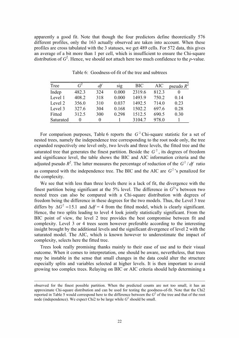
22

apparently a good fit. Note that though the four predictors define theoretically 576 different profiles, only the 163 actually observed are taken into account. When these profiles are cross tabulated with the 3 statuses, we get 489 cells. For 572 data, this gives an average of a bit more than 1 per cell, which is insufficient to ensure the Chi-square distribution of G2. Hence, we should not attach here too much confidence to the p-value.

Table 6: Goodness-of-fit of the tree and subtrees

Tree G2 df sig BIC AIC pseudo R2 Indep 482.3 324 0.000 2319.6 812.3 0 Level 1 408.2 318 0.000 1493.9 750.2 0.14 Level 2 356.0 310 0.037 1492.5 714.0 0.23 Level 3 327.6 304 0.168 1502.2 697.6 0.28 Fitted 312.5 300 0.298 1512.5 690.5 0.30 Saturated 0 0 1 3104.7 978.0 1

For comparison purposes, Table 6 reports the 2G Chi-square statistic for a set of

nested trees, namely the independence tree corresponding to the root node only, the tree expanded respectively one level only, two levels and three levels, the fitted tree and the saturated tree that generates the finest partition. Beside the 2G , its degrees of freedom and significance level, the table shows the BIC and AIC information criteria and the adjusted pseudo R2. The latter measures the percentage of reduction of the dfG /2 ratio as compared with the independence tree. The BIC and the AIC are 2G ’s penalized for the complexity.

We see that with less than three levels there is a lack of fit, the divergence with the finest partition being significant at the 5% level. The difference in G2’s between two nested trees can also be compared with a Chi-square distribution with degrees of freedom being the difference in these degrees for the two models. Thus, the Level 3 tree differs by 15.1=∆ 2G and ∆df = 4 from the fitted model, which is clearly significant. Hence, the two splits leading to level 4 look jointly statistically significant. From the BIC point of view, the level 2 tree provides the best compromise between fit and complexity. Level 3 or 4 trees seem however preferable according to the interesting insight brought by the additional levels and the significant divergence of level 2 with the saturated model. The AIC, which is known however to underestimate the impact of complexity, selects here the fitted tree.

Trees look really promising thanks mainly to their ease of use and to their visual outcome. When it comes to interpretation, one should be aware, nevertheless, that trees may be instable in the sense that small changes in the data could alter the structure especially splits and variables selected at higher levels. It is then important to avoid growing too complex trees. Relaying on BIC or AIC criteria should help determining a

observed for the finest possible partition. When the predicted counts are not too small, it has an approximate Chi-square distribution and can be used for testing the goodness-of-fit. Note that the Chi2 reported in Table 5 would correspond here to the difference between the G2 of the tree and that of the root node (independence). We expect Chi2 to be large while G2 should be small.

23

somewhat robust tree. Splits behind the optimal BIC or AIC will be less reliable and their interpretation requires then more caution.

4 Conclusion This paper stressed the scope and limits of various methods available for analyzing life course data globally, and especially in demography. Demographers and historical demographers invented their own longitudinal analytical tools like the life tables or the family reconstitution, almost since the birth of their discipline. However, everywhere but probably more in the French-speaking areas, those sciences of the masses hesitated to make the step further, while they were so close from the life course perspective and methods. Many academics are still living this transition… For the practitioners of highly quantitative sciences, we did not hide the complexity of the new approaches and wanted to both introduce and illustrate promising methodological perspectives. In the same time, we did not elaborate this contribution only for our disciplinary fellows, since one of the most important evolutions is that the analytical techniques obviously lend us to neighboring disciplines that share the same tools and explore similar concepts, giving to the interdisciplinary ambition a growing substance.

We choose to illustrate different approaches, and especially the emerging data mining techniques that should be able to provide original additional insights on results provided by more classical statistical methods. The discussion, however, is by no means exhaustive. Among the techniques we did not discuss, optimal matching (Abbot and Forrest, 1986; Malo and Munoz, 2003) deserves special attention. Optimal matching is, like Markovian models, a state sequence analysis tool. It is merely a data mining approach, since it proceeds heuristically. Unlike the mining of frequent sequences that does not care about the similarity between sequences, optimal matching is concerned with the discovering of similarities between sequence patterns. Optimal matching evaluates the proximity between two sequences by seeking the minimal number of changes that can transform a sequence a into a sequence b. Survival (Ciampi et al., 1988; Segal, 1988) and risk trees (Leblanc and Crowley, 1992) developed in the field of biomedicine during the first half of the 90’s would also merit further attention from historians and demographers.

It is worth mentioning that the statistical and data mining approaches are not substitutes for one another. They are complementary, each method bringing its own insight. The choice of a method will be dictated by the kind of data available: spell durations, event sequences, state sequences, and indeed the type of results expected: knowledge about probability of transitions, effects on these risks, characteristic trajectories or life sequences. Another important element for this choice, at least for the end user, is the availability of user-friendly softwares and the level of expertise required to run the method and interpret the results. Many softwares propose duration or hazard models and/or classification trees. It is less obvious to find friendly tools for Markov models and the mining of sequential rules. March 2 is a promising solution for Markov models, while specialized softwares like Clementine propose sequence mining tools (see http://www.kdnuggets.com for a list of commercial and free data mining softwares). The use and interpretation of hazard models is very similar to that of other regression like models, which renders them attractive. The interpretation of induction trees is also very straightforward and looks therefore as a promising tool. Nevertheless, the fine tuning of trees, which may be highly instable, requires generally more care than

24

hazard models. Mining frequent sequential patterns requires also some experience to get interesting patterns. In any case, the new highlights provided by these data mining approaches are worth the effort.

References

Abbot, A. and J. Forrest (1986). Optimal matching methods for historical sequences. Journal of Interdisciplinary History 16, 471–494.

Agrawal, R. and R. Srikant (1994, September). Fast algorithm for mining association rules in large databases. In Proceedings 1994 International Conference on Very Large Data Base (VLDB’94), Santiago, Chile, pp. 487–499.

Agrawal, R. and R. Srikant (1995). Mining sequential patterns. In Proceedings of the International Conference on Data Engeneering (ICDE), Taipei, Taiwan, pp. 487–499.

Allison, P. D. (1982). Discrete-time methods for the analysis of event histories. In S. Lienhardt (Ed.), Sociological Methodology, pp. 61–98. San Francisco: Jossey-Bass Publishers.

Alter, G., M. Oris, and G. Broström (2001). The family and mortality: A case study from rural Belgium. Annales de la démographie historique 1, 11–31.

Alter, G. and M. Oris (2000). Mortality and economic stress: Individual and household responses in a nineteenth-century Belgian village. In T. Bengtsson O. Saito (Eds.), Population and Economy: From Hunger to Modern Economic Growth, pp. 335–370. Oxford: Oxford University Press.

Alter, G. (1998). L’event history analysis en démographie historique: difficultés et perspectives. Annales de Démographie historique 2, 23–3.

Aranza-Ordaz, F. J. (1983). An extension of the proportional hazards model for grouped data. Biometrics 39, 109-117.

Barber, J. S., S. A. Murphy, W. G. Axinn, and J. Maples (2000). Discrete-time multilevel hazard analysis. In M. E. Sobel M. P. Becker (Eds.), Sociological Methodology, 30, pp. 201–235. New York: The American Sociological Association.

Beekink, E., F. van Poppel and A. C. Liefbroer (1999). Surviving the loss of the parent in a nineteenth-century Dutch provincial town. Journal of Social History 32, 614-670.

Berchtold, A. and A. Berchtold (2004). MARCH 2.01: Markovian model computation and analysis. User’s guide, www.andreberchtold.com/march.html.

Berchtold, A. and A. E. Raftery (2002). The mixture transition distribution model for high-order Markov chains and non-gaussian time series. Statistical Science 17(3), 328–356.

Berchtold, A. (1999). The double chain Markov model. Communications in Statistics: Theory and Methods 28(11), 2569–2589.

Berchtold, A. (2001). Estimation in the mixture transition distribution model. Journal of Time Series Analysis 22(4), 379–397.

25

Berchtold, A. (2002). High-order extensions of the double chain Markov model. Stochastic Models 18(2), 193–227.

Berquo, E. and P. Xenos (1992). Editor’s introduction. In E. Berquo P. Xenos (Eds.), Family systems and cultural change, pp. 8–12. Oxford: Clarendon Press.

Billari, F. C., J. Fürnkranz, and A. Prskawetz (2000). Timing, sequencing, and quantum of life course events: a machine learning approach. Working Paper 010, Max-Plank-Institute for Demographic Research, Rostock.

Blockeel, H., L. Dehaspe, J. Ramon, and J. Struyf (2004). The ACE data mining system. User’s manual, Katholieke Universiteit Leuven, Leuven.

Blockeel, H., J. Fürnkranz, A. Prskawetz, and F. Billari (2001). Detecting temporal change in event sequences: An application to demographic data. In L. D. Raedt A. Siebes (Eds.), Principles of Data Mining and Knowledge Discovery: 5th European Conference, PKDD 2001, Volume LNCS 2168, pp. 29–41. Freiburg in Brisgau: Springer.

Blossfeld, H.-P., A. Hamerle, and K. U. Mayer (1989). Event history analysis, Statistical theory and application in the social sciences. Hillsdale NJ: Lawrence Erlbaum.

Blossfeld, H.-P. and G. Rowher (2002). Techniques of Event History Modeling, New Approaches to Causal Analysis (2nd ed.). Mahwah NJ: Lawrence Erlbaum.

Bocquier, P. (1996). L’analyse des enquêtes biographiques à l’aide du logiciel STATA. Paris: Centre français sur la population et le développement.

Bourdieu, P. (1986). L'illusion biographique. Actes de la Recherche en Sciences sociales 62-63, 69-72.

Breiman, L. (2001). Satistical modeling: The two cultures (with discussion). Statistical Science 16 (3), 199-231.

Breiman, L., J. H. Friedman, R. A. Olshen, and C. J. Stone (1984). Classification And Regression Trees. New York: Chapman and Hall.

Bryk, A., S. W. Raudenbush, and R. Congdon (1996). HLM: Hierarchical Linear and Nonlinear Modeling with the HLM/2l and HLM/3l Programs. Chicago: Scientific Software International.

Caselli, G., J. Vallin and G. Wunsch (Eds.) (2001). Démographie : analyse et synthèse, vol. I. La dynamique des populations. Paris: Institut national d'études démographiques.

Ciampi, A., S. A. Hogg, S. McKinney, and J. Thiffault (1988). RECPAM: a computer program for recursive partitioning and amalgamation for censored survival data and other situations frequently occuring in biostatistics i. methods and program features. Computer Methods and Programs in Biomedicine 26(3), 239–256.

Courgeau, D. and E. Lelièvre (1993). Event History Analysis in Demography. Oxford: Clarendon Press.

Cox, D. R. (1972). Regression models and life-tables. Journal of the Royal Statistical Society, Series B 34(2), 187–220.

Demeny, P. and G. McNicoll (eds.) (2003). Encyclopedia of Population. New York: McMillan, 2 vol.

26

De Rose, A. and A. Pallara (1997). Survival trees: An alternative non-parametric multivariate technique for life history analysis. European Journal of Population 13, 223–241.

Dupâquier, J. and M. Dupâquier (1985). Histoire de la démographie. Paris: Perrin. Dykstra, P. and L. J. G. van Wissen (1999). Introduction: the life course approach as an

interdisciplinary framework for population studies. In L. J. G. van Wissen and P. Dykstra (Eds.), Population Issues. An Interdisciplinary Focus, pp. 1–22. New York: Plenum Press.

Goldstein, H., J. Rasbash, I. Plewis, D. Draper, W. Browne, M. Yang, G. Woodhouse, and M. Haely (1998). A user guide to MLwiN. Technical report, Multilevels Models Project, London.

Greenhalgh, S. (1996), The social construction of population science: an intellectual, institutional and political history of twentieth-century demography, Comparative Studies in Society and History 38, 1, 26-66.

Hagestad, G. O. (2003). Interdependent lives and relationships in changing times. a life course view of families and aging. In R. A. H. Settersten (Ed.), Toward New Understanding of Later Life, pp. 135–160. Amytiville-New York: Baywood Publishing.

Hand, D. J., H. Mannila, and P. Smyth (2001). Principles of Data Mining (Adaptive Computation and Machine Learning). Cambridge MA: MIT Press.

Han, J. and M. Kamber (2001). Data Mining: Concept and Techniques. San Francisco: Morgan Kaufmann.

Hogdson, D. (1988), Demography as social science and policy science, Population and development review 9, 1, 541-569.

Hogdson, D. (1991), The ideological origins of the Popualtion Association of America, Population and Development Review 17, 1, 1-34.

Höhn, C. (1992). The IUSSP programme in family demography. In E. Berquo and P. Xenos (Eds.), Family systems and cultural change, pp. 3–7. Oxford: Clarendon Press.

Holford, T. R. (1980). The analysis of rates and survivorship using log-linear models. Biometrics 65, 159–165.

Kass, G. V. (1980). An exploratory technique for investigating large quantities of categorical data. Applied Statistics 29(2), 119–127.

Kish, L. and M. R. Frankel (1974). Inference from complex samples (with discussion). Journal of the Royal Statistical Societey, Series B 36, 1–37.

Landwehr, N., M. Hall, and E. Frank (2003). Logistic model trees. In N. Lavrac, D. Gamberger, L. Todorovski, H. Blockeel (Eds.), Machine Learning: ECML 2003, Volume 2837 of LNAI, pp. 241–252. Springer.

Leblanc, M. and J. Crowley (1992). Relative risk trees for censored survival data. Biometrics 48, 411–425.

Lillard, L. A. (1993). Simultaneous equations for hazards: Marriage duration and fertility timing. Journal of Econometrics 56, 189–217.

Lin, D. Y. and L. J. Wei (1989). The robust inference for the Cox proportional hazards model. Journal of the American Statistical Association 84, 1074–1078.

27

Lynch, K.A. (1998). Old and new research in historical patterns of social mobility. Historical Methods 31(3), 93-98.

MacDonald, I. L. and W. Zucchini (1997). Hidden Markov and Other Models for Discrete-Valued Time Series. London: Chapman and Hall.

Malerba, D., A. Appice, M. Ceci, and M. Monopoli (2002). Trading-off local versus global effects of regression nodes in model trees. In M.-S. Hacid, Z. W. Ras, D. A. Zighed, Y. Kodratoff (Eds.), Foundations of Intelligent Systems, ISMIS 2002, Volume 2366 of LNAI, pp. 393–402. Springer.

Malo, M. A. and F. Munoz (2003). Employment status mobility from a lifecycle perspective: A sequence analysis of work-histories in the bhps. Demographic Research 9(7), 471–494.

Mannila, H., H. Toivonen, and A. I. Verkamo (1997). Discovery of frequent episodes in event sequences. Data Mining and Knowledge Discovery 1(3), 259–289.

Mannila, H., H. Toivonen, and A. I. Verkamo (1994, July). Efficient algorithms for discovering association rules. In Proceedings AAAI’94 Workshop Knowledge Discovery in Databases (KDD’94), Seattle, WA, pp. 181–192.

McCullagh, P. and Nelder, J. A. (1989). Generalized Linear Models. London: Chapman and Hall.

Oris, M. and M. Poulain (2003). Entre blocages spatiaux et nouvelles dynamiques familiales: quitter ses parents. In Populations et défis urbains. Chaire Quetelet 1989, pp. 313–337. Louvain-la-Neuve: Academia-Bruylant/L’Harmattan.

Oris, M., G. Ritschard, and A. Berchtold (2003, November). The use of Markov process and induction trees for the study of intergenerational social mobility in nineteenth century Geneva. In Social Science History Association Annual Meeting, Baltimore.

Paliwal, K. K. (1993). Use of temporal correlation between successive frames in a hidden Markov model based speech recognizer. Proceedings ICASSP 2, 215–218.

Quinlan, J. R. (1986). Induction of decision trees. Machine Learning 1, 81–106. Quinlan, J. R. (1993). C4.5: Programs for Machine Learning. San Mateo: Morgan

Kaufmann. Rabiner, L. R. (1989). A tutorial on hidden Markov models and selected applications in

speech recognition. Proceedings of the IEEE 77(2), 257–286. Raftery, A. E. and S. Tavaré (1994). Estimation and modelling repeated patterns in high

order Markov chains with the mixture transition distribution model. Applied Statistics 43, 179–199.

Ritschard, G. and D. A. Zighed (2003). Goodness-of-fit measures for induction trees. In N. Zhong, Z. Ras, S. Tsumo, E. Suzuki (Eds.), Foundations of Intelligent Systems, ISMIS03, Volume LNAI 2871, pp. 57–64. Berlin: Springer.

Rohwer, G. and U. Pötter (2002). TDA user’s manual. Software, Ruhr-Universität Bochum, Fakultät für Sozialwissenschaften, Bochum.

Ryczkowska, G. and G. Ritschard (2004, March). Mobilités sociales et spatiales: Parcours intergénérationnels d’après les mariages genevois, 1830-1880. In Fifth European Social Science History Conference, Berlin.

Segal, M. R. (1988). Regression trees for censored data. Biometrics 44, 35–47. SPSS (Ed.) (2001). Answer Tree 3.0 User’s Guide. Chicago: SPSS Inc.

28

Szreter, S. (1993). The idea of demographic transition: a critical intellectual history. Population and Development Review 19, 659-701.

Therneau, T. M. and P. M. Grambsch (2000). Modeling Survival Data. New York: Springer.

Vallin, J. (2001). Populations et individus. In G. Caselli, J. Vallin and G. Wunsch (Eds.), Démographie : analyse et synthèse, vol. I. La dynamique des populations, pp. 9-12. Paris: Institut national d'études démographiques.

Van de Kaa, D. J. (1996), Anchored narratives : the story and findings of half a century of research into the determinants of fertility, Population Studies, 50, 3, 389-432.

Van Imhoff, E., A. Kuijsten, P. Hooimeijer, and L. J. G. van Wissen (1995). Household demography and household modeling. New York: Kluwer - Plenum Press.

Vaupel, J.W., K.G. Manton, E. Stallard (1979). The impact of heterogeneity in individual frailty on the dynamics of mortality. Demography 16, pp. 439-454.

Véron, J. (1993). Arithmétique de l’homme: la démographie entre science et politique. Paris: Editions du Seuil.

Willekens, F. J. (1999). The life course: Models and analysis. In L. J. G. van Wissen, P. Dykstra (Eds.), Population Issues. An Interdisciplinary Focus, pp. 23–51. New York: Plenum Press.

Yamaguchi, K. (1991). Event history analysis. ASRM 28. Newbury Park and London: Sage.

Zighed, D. A. and R. Rakotomalala (1996). SIPINA-W(c) for Windows. User’s guide, Laboratory ERIC - University of Lyon 2, Lyon.