Let's Design Algorithms for VLSI Systems - …caltechconf.library.caltech.edu/192/1/HTKung.pdfLet's Design Algorithms for VLSI Systems H. T. Kung Department of Computer Science Carnegie-Mellon

Let's Design Algorithms for VLSI Systems

H. T. Kung

Department of Computer Science Carnegie-Mellon University

Pittsburgh, Pennsylvania 15213

January 1979

G5

This r esear ch is supported in part by the National Science Foundation under Grant MCS 75-222-55 and the Office of Naval Research under Contract N00014- 76-C- 0370, NR 044- 422.

CALTECH CONFERENCE ON VLS I , January 1979

66 H.T. Kun g

1. Introduction

Very Large Scale Integration (VLSI) technology offers the potential of implementing

complex algorithms directly in hardware [Mead and Conway 79). This paper (i) gives

examples of algorithms that we believe are suitable for VLSI implementation, (ii) provides a

taxonomy for algorithms based on their communication structures, and (iii) discusses some

of the insights that are beginning to emerge from our efforts in designing algorithms for

VLSI sys tems.

To illustrate the kind of algorithms in which we are interested, we first review, in Section

2, the matrix multiplication algorithm in [Kung and Leiserson 78] which uses the hexagonal

array a5 it5 communication geometry. In Section 3, we discuss issues in the design of VLSI

algorithm!>, and classify algorithms according to their communication geometries. Sections 4

to 7 represent an attempt to characterize computations that match various processor

interconnection schemes. Special attention is paid to the linear array connection, since it is

the simplest communication structure to build and is fundamental to other structures. Some

concluding remarks are given in the last section.

2. A Hexagonal Processor Array for Matrix Multiplication --- An Example

Le t A = (a1j) and B = (b1J) be n x n band matrices with band width w 1 and w2

, respectively.

Thei r product C = (c11) can be computed in 3n + min(wl' w2) units of time by an array of

w 1w 2 hexagonally connected "inner product step processors". Note that computing C on a

uniprocessor using the standard algorithm would req\,Jire time proportional to O(w1w 2n). As

shown in Figure 1, an inner product step processor updates c by c ~ c + ab and passes

data a, b at each cycle.

c

a:Q:b ,.. •'

b ... 1

'a

c

a ~ a b ~ b c ~ c + ab

Figure l: The inner product step processor for the hexagonal processor array in Figure 3 .

INVITED SPEAKERS SESSION

Le t's Design Al gorithms fo r VLS I Systems 67

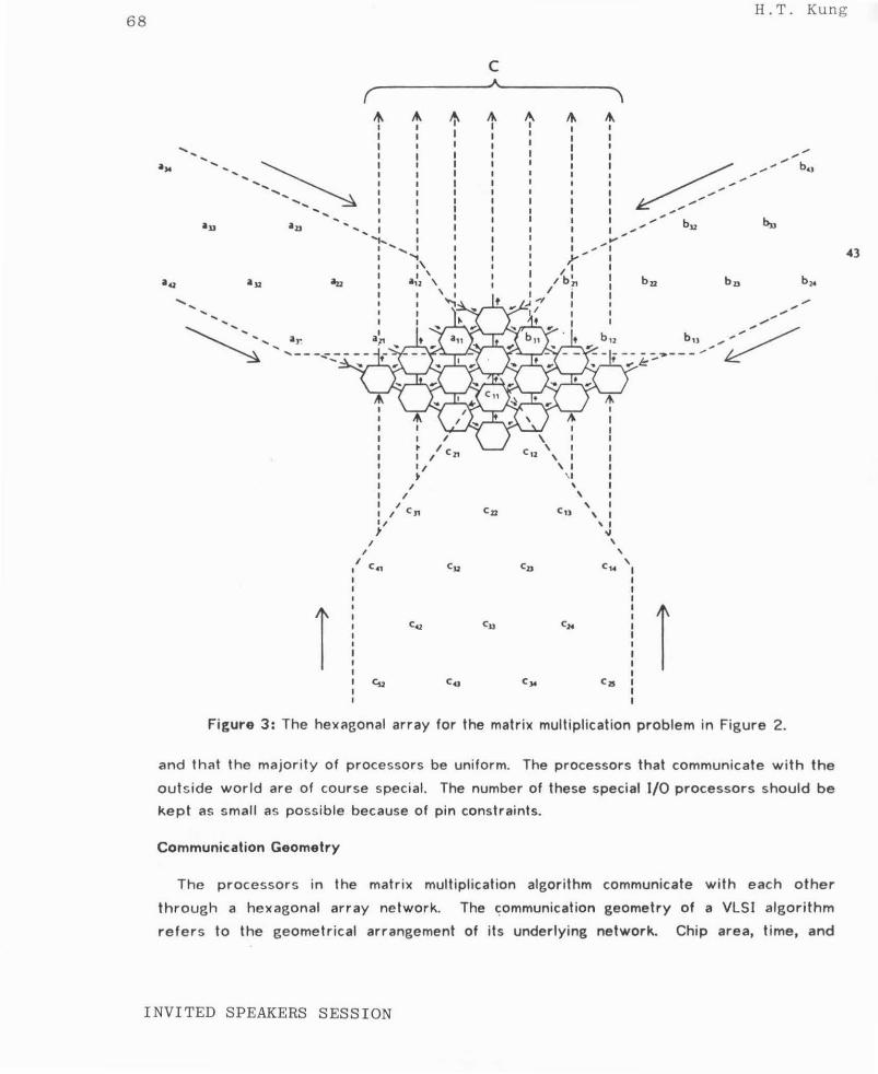
We illustrate the computation on the hexagonal array by considering the band matrix

multiplication problem in Figure 2.

a .. a 11

0 b ll b l7 b iJ

0 c" c 12 c 13 c 14 0

a7, an an b21 bn b7J b74 c 21 c 22 r. 2J r. 2~

aJ , a :'l7 a :~:~ a J~ bJl bJJ bl4

b,. J ~:~ r. J} r. Jl r. J~

a ~1 b42 c•z

0 0

Figure 2: Band matrix multiplication.

The diamond shaped hexagonal array for this case is shown in Figure 3, where arrows

indicate the direction of the data flow. The elements in the bands of A, 8 and C march

synchronously through the network in three directions. Each cij is initialized to zero as it

enters the network through the bottom boundaries. (For the general problem of computing

C=AB+D where D=(dij) is any given matrix, each cij should be initialized to the

corresponding d ij·) One can easily see that each cij is able to accumulate all its terms

before it leaves the network through the upper boundaries.

3. The Structure of VLSI Algorithms

3 .1. Three Attributes of a VLSI Algorithm

There are three important attributes of the matrix multiplication algorithm described in

the preceding section, or of any VLSI algorithm in general. In the following, we discuss

these attributes. We also suggest how an algorithm well -suited for VLSI implementation

will appear in terms of these attributes.

Function of each processor

A processor may perform any constant-time operation such as an inner product step, a

comparison-exchange, or simply a passage of data. For implementation reasons, it is

desi r ab le that the logic and storage requirement at each processor be as small as possible

CALTECH CONFERENCE ON VLSI, January 1979

68

........ I '.._ I ....

1\ I ' au \ I

.......... I .... I

I

I I

II Cn

; I

I I

I c.,

c4.1

Cu

"' I I I I I

cu

Co

H.T. Kung

c

I I

cu I I

\ I

" ' \ Czz CtJ ' ' 'I

'>J

' ' Cn c,. '

cu cl4 r cJ< cl5

figure 3: The hex;~gonal array for the matrix multiplication problem in figure 2.

and that the majority of processors be uniform. The processors that communicate with the

outside world are of course specia l. The number of these special 1/0 processors should be

kept as small as possible because of pin constraints.

Communication Geometry

The processors in the matrix multiplication algorithm communicate with each other

through a hexagonal array network. The c;ommunication geometry of a VLSI algorithm

refers to the geometrical arrangement of its underlying network. Chip area, time, and

INVITED SPEAKERS SESS ION

Let's Design Algorithms for VLSI Systems 69

power required for implementing an algorithm are largely dominated by the communication

geometry of the algorithm [Sutherland and Mead 77]. It is essential that the geometry of

an algorithm be simple and regular because such a geometry leads to high density and,

more importantly, to modular design. There are few communication geometries which are

trul y simple and regular. For example, there are only three regular figures -- the square,

the hexagon, and the equilateral triangle -- which will close pack to completely cover a

two - d imensional area. The remainder of the paper deals mainly with algorithms with simple

and regular communication geometries.

Data Movement

The manner in which data circulates on the underlying network of processors is a critical

aspect of a VLSI algorithm. Pipelining, a form of computation frequently used in VLSI

algorithms, is an example of data movement. Conceptually, it is convenient to think of data

as moving synchronously, although asynchronous implementations may sometimes be more

attractive. Data movement is characterized in at least the following three dimensions:

direction, speed, and timing. An algorithm can involve data being transmitted in different

directions at different speeds. The timing refers to how data items in a data stream should

be configured so .that the right data will reach the right place at the right time. Consider,

for example, the matrix multiplication algorithm in Figure 3. There are three data streams,

consisting of entries in matrices A, 8, and C. The data streams move at the same speed in

three directions, and elements in each diagonal of a matrix are separated by three time

units. To reduce the complexity in control, it is important that data movements be simple,

regular , and uniform.

3.2. Systolic Systems

It is instructive to view a VLSI algorithm as a circulatory system where the function of a

processor is analogous to that of the heart. Every processor rhythmically pumps data in

and out, each time performing some short computation, so that a regular flow of data is

kept up in the network. In (Kung and Leiserson 78], a network of (identical) simple

processors that circulate data in a regular fashion is called a systolic system. (The word

"systole", borrowed from physiologists, originally refers to the recurrent contractions of

the heart and arteries which pulse blood through the body.) Systolic computations are

characterized by the strong emphasis upon data movement, pipelining In particular. VLSI

algorithms are examples of systolic systems.


70 H.T. Kun g

3 .3. A Taxonomy for VLSI algorithms

We give a taxonomy for VLSI algorithms based on their communication geometr ies. This

taxonomy prov ides a framework for characterizing computations on the basis of their

communication structures. The table on the next page provides examples of algorithms

classi fied by the taxonomy. Most of these algorithms will be discussed in subsequent

sections of this paper.

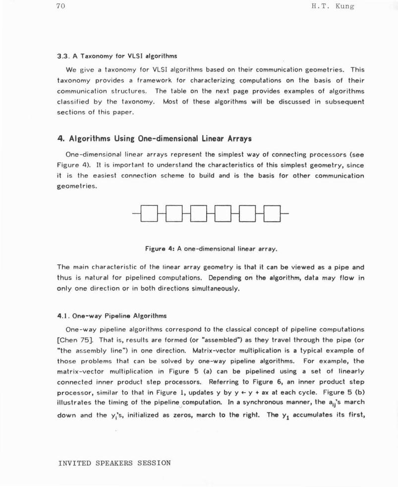
4. Algorithms Using One-dimensional Linear Arrays

One -dimens i~nal linear ar rays represent the simplest way of connecting processors (see

Figure 4). It is important to understand the characteristics of this simplest geometry, since

it is the easiest connection scheme to build and is the basis for other communication

geometries.

Figure 4: A one-dimensional linear array.

The main characteristic of the linear array geometry is that it can be viewed as a pipe and

thus is natural for pipelined computations. Depending on the algorithm, data may flow in

only one direction or in both directions simultaneously.

4 .1 . One-way Pipeline Algorithms

One - way pipeline algorithms correspond to the classical concept of pipeline computations

[Chen 75]. That is, results are formed (or "assembled") as they travel through the pipe (or

"the assembly line") in one direction. Matrix-vector multiplication is a typical example of

those problems that can be solved by one-way pipeline algorithms. For example, the

matrix-vector multiplication in Figure 5 (a) can be pipelined using a set of linearly

connected inner product step processors. Referring to Figure 6, an inner product step

processor, similar to that in Figure 1, updates y by y ..- y + ax at each cycle. Figure 5 (b)

illustrates the timing of the pipeline._.computation. In a synchronous manner, the a1/s march

down and the y1's, initialized as zeros, march to the right. The y1 accumulates its first,

I NVITED SPEAKERS SESSION

·Let's Design Algorithms for VLSI Systems 71

Examples of VLSI Algorithms

Communication Geometry

1-dim linear arrays

2-dim square arrays

2-dim hexagonal arrays

Trees

Examples

Matrix-vector multiplication FIR filter Convolution OFT Carry pipelining Pipeline arithmetic units

Real-time recurrence evaluation Solution of triangular linear systems Constant-time priority queue, on-line sort Cartesian product Odd-even transposition sort

Dynamic programming for optimal parenthesization

Numerical relaxation for POE Merge sort FFT Graph algorithms using adjacency

matrices

Matrix mult iplication Transitive closure LU-decomposition by Gaussian

elimination without pivoting

Searching algorithms Queries on nearest neighbor, rank, etc. NP-complete problems

systolic search tree Parallel function evaluation Recurrence evaluation

Shuffle- exchange networks FFT Bitonic sort


72 H.T. Kung

a I 1

a 12

a 13

X 1 yl

a 33

a a a X y2 21 22 23 2 = a a 32 23

a a a X y3 31 32 33 3 a a a

31 22 13

a ~u a 42

a 43 y4 ~

821

812

a a a y5 ~ ~ 51 52 53 8

II

y y 2 l

X I )( 2

)(

3

(a) (b)

Figure 5: (a) Matrix-vector multiplication and (b) one-way pipeline compution.

a

y ._ y + ax

X

Figure 6: The inner product step processor for the linear array in Figure 5 (b).

second, and third terms at time 1, 2, and 3, respectively, whereas the y2 accumulates its


J.et's Design Al gorithms for VLSI Systems 73

first, second, and third terms at time 2, 3, and 4, respectively. Thus, this is a (left-to-right)

one-way pipeline computation. In the figure, the x1's are underlined to denote the fact that

the same x1

is fed into the processor at each step in the computation (so x1

can actually be

a canst ant stored in the processor). This notation will be used throughout the paper.

Any problem involving a set of independent multi-stage computations of the same type

can be viewed as a matrix-vector multiplication. That is, each independent computation

corresponds to the computation of a component in the resulting vector, and each stage of

the com put at ion corresponds to an "inner product step" of the form y +- F(a,x,y) . for some

function F. Consequently, with linearly connected processors capable of performing these

functions F, the problem can be solved rapidly by a one-way pipeline algorithm. Other

examples of one-way pipeline algorithms include the carry pipelining for digit adders (see

e.g., [Hallin and Flynn 72]) and pipeline arithmetic units (see e.g., [Ramamoorthy and Li 77]).

4.2. Two-way Pipeline Algorithms

There are inherent reasons why some problems can only be solved by pipeline

algorithms using two-way data flows. We illustrate these reasons by examining three

problems: band matrix-vector multiplication, recurrence evaluation, and priority queues.

Band Matrix-vector Multiplication

The band matrix-vector multiplication, for example, in Figure 7 differs from that in Figure

5 (a) in that the band in the matrix, the vector x, and the vector y can all be arbitrarily

long. Thus, to solve the problem on a finite number of processors, all three quantities must

move during the computation. This leads to the algorithm in Figure 8 (a), which uses the

inner product step processor in Figure 8 (b). The x1's and y1's march in opposite directions,

so that each x1 meets all the y1's. Notice that the x1's are separated by two time units, as

are the y 1's and the diagonal elements in the matrix. One can easily check that each y 1,

initialized as zero, is able to accumulate all of its terms before it leaves the left-most

processor.

A s imple conclusion we can draw from this example is that if the size of the input and

the output of a problem are larger than the size of the network, then all the inputs and

intermediate re sults have to move during the computation. In this case, to achieve the

greatest possible number of interactions among data we should let data flow in both

directions simultaneously.


74 H .T . Kun g

a" a 11 x, y,

a?, an an 0 x7 Yz

al, al7 all al. XJ YJ

a.? a.l a •• a.5 x. Y.

a5l

l 0

Figure 7: Band matrix-vector multiplication.

In reference to Figure 8 <?>, since a two-way pipeline algorithm makes each x1 meet all

the y 1's, it can compute the Cartesian product of the vectors x and y in parallel on a linear

array. In this case, the a1j, initialized as zero, is output from the bottom of the

corresponding processor with a value resulting from some combination of x1 and Yr

Matrix multiplication (or band matrix-vector multiplication) is of interest in its own right.

Moreover many important computations such as convolution, discrete Fourier transform and

finite impulse response filter are special instances of matrix-vector multiplications, and

hence can be solved in parallel on linear processor arrays. For details, see [Kung and

Leiserson 78].

Recurrence Evaluation

Many computational tasks are concerned with evaluations of recurrences. A k-th order

recurrence problem is defined as follows: Given x0, x_l' ... ,x_k+l' we want to evaluate xl' x 2,

... , defined by

where the R1's are given "recurrence functions". Parallel evaluation of recurrences is


Le t's Des i g n Al gorithms fo r VLS I Systems

a a 23 32

~ ~ ~ ~ a

22 a

31

~ ~ ~ ~ a

12 a

21 (a)

~ ~ ~ ~ a

11

X 2~ y2

a

X +- )( (b) y +- y + ax

Figuro 8: (a} A two-way pipeline computation for the band matrix-vector multiplication in Figure 7, and (b) the inner product step processor used.

75

interesting and challenging, since the recurrence problem on the surface appears to be

highly sequential. We show that for a large class of recurrence functions, a k-th order

recurrence problem can be solved in real-time on k linearly connected processors. That is,

a new x1 is output every constant period of time, independent of k. To illustrate the idea,

we consider the following liMear recurrence:

(2)

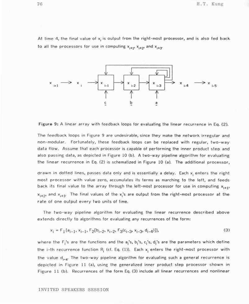
where the a, b, c, and d are constants. It is easy to see that feedback links are needed for

evaluating such a recurrence on a linear array, since every newly computed term has to be

used later for computing other terms. A straightforward network with feedback loops for

evaluating the recurrence is depicted in Figure 9, where each processor, except the

right-most one which has more than one output port, is the inner product step processor of

Figure 6. The x1, initialized as d, gets cxt-3, bx1_ 2, and axl-1 at time 1, 2, and 3, respectively.

CALTECH CONFERENCE ON VLS I, J a nua r y 1979

7 6 H.T . Kung

At time 4, the final value of x1 is output from the right-most processor, and is also fed back

to all the processors for use in computing x1+1, x1+2, and x1+3"

X -::> X X X X X ~ X i+ 1 i-1 i-2 i-3 i-4 i-5

t c b a - - -

Figure 9: A linear array with feedback loops for evaluating the linear recurrence in Eq. (2).

The feedback loops in Figure 9 are undesirable, since they make the network irregular and

non- modular. Fortunately, these feedback loops can be replaced with regular, two-way

data flow. Assume that each processor is capable of performing the inner product steo and

also passing data, as depicted in Figure 10 (b). A two-way pipeline algorithm for evaluating

the linear recurrence in Eq. (2) is schematized in Figure 10 (a}. The additional processor,

drawn in dotted lines, passes data only and is essentially a delay. Each x1 enters the right

most processor with v alue zero, accumulates its terms as marching to the left, and feeds

back its final value to the array through the left-most processor for use in computing x1+ 1,

x1+2, and x1+3• The final values of the x1's are output from the right-most processor at the

rate of one output every two units of time.

The two-way pipeline algorithm for evaluating the linear recurrence described above

extends directly to algorithms for evaluating any recurrences of the form:

(3)

where the Fi's are the functions and the ai's, bi's, ci's, di's are the parameters whiclrl define

the i-th recurrence function Ri (cf. Eq. (1 }). Each x1 enters the right-most processor with

the v alue d1_

4• The two-way pipeline algorithm for evaluating such a general recurrence is

depicted in Figure 11 (a), using the generalized inner product step processor shown in

Figure 11 (b). Recurrences of the form Eq. (3) include all linear recurrences and nonlinear


Let's Design Algorithms for VLSI Systems

(a) X I i-2 I I ____ _

(b) X

y

a

X

y

xi-4 ~ X ~

X +-X

v +-- y + ax

77

X i-5 X

i+l

Figure 10: (a) A two-way p ipeline algorithm for evaluating the linear recurrence in Eq. (2), and (b) the inner product step processor.

(a)

(b)

F F F 1 2 3

X i-4 ~ ~ X i-5 X X ~ ~ X

i-2 I i+l ----- ( - d ) (-d ) i-4 i-3

a b c i- 1 i-2 i- 3

x+-x

y +-- F(a,x,y)

a

Figure 11: (a) A two-way pipeline algorithm for evaluating the general recurrence in Eq. (3), and (b) the generalized inner product step processor.

ones such as


7 8 H.T. Kung

x i = 3xf_1 + xi_ 2 * sin(xi_3 + 4). (4)

Eq. (4) corresponds to the case where F3(x, y, z) = sin(y + z) with z=4, F2( x, y, z) = y * z,

and F 1 (x, y , z) = 3y 2 + z. In fact, Eq. (3) is not yet the most general form of recurrence

that linear processor arrays can ev aluate in real-time. For example, the generalized inner

prodw-t !>h='! p p r OC'P.SSOr in FietJrP. 1 I (b) Ci'ln b(! fwther e(!nP.ri'lli7(!d to incltJcie the <;: i=lp::~bility

of updating both x and y. That is, the processor performs x +- F(l)(a,x,y) and y +- F(2)(a,x,y)

according to some given functions F(l), F<2>. Gi ven a linear array of such generalized inner

product step processors, it is often an interesting and nontrivial task to figure out what

recurrence the array actually ev aluates. Here we note without proof that the problem can

always be sol ved in principle at least by using induction on the number of processors in

the array.

We conclude our discussion of recurrence evaluation by stating that two-way pipelining

is a powe rful construct in the sense that it can eliminate the need for using undesirable

feedback loops such as those encounter in Figure 9.

Priority Queues

A data structure that can process INSERT, DELETE, and EXTRACT_MIN operations is called a

priority queue. Priorit y queues are bas ic structures used in many programming tasks. If a

prio rit y queue is implemented b y some balanced tree, for example a 2-3 tree, then an

operation on the queue will typically take O(log n) time when there are n elements stored

in the tree [Aho e t a!. 75]. Thi s O(log n) delay can be replaced w ith a constant de lay if a

line ar array of processors is used to implement the priority queue. Here we shall only

sketch the basic idea behind the linear array implementation. A complete description will

be reported in another paper.

To v i s u;:~li 7P. thP. o:~leorithm , wP. o:~s~umP. that thfi'! lin!;'!ar ~rray in Fieure 4 has bee11 phys icall y rotated 90° and that processors are capable of performing comparison-exchange

ope rations on elements in neighboring processors. We try to maintain elements in the

arr ay in sorted order according to their weights. After an element is inserted into the

array fro m the top, it will "sink down" to the proper place by trading positions with

elements hav ing smaller weights (so lighter elements will "bubble up"). To delete an

element, we insert an "anti -element" which first sinks down from the top to find the

element , then annihilates it. Elements below can then bubble up into the empty processor.

Hence the e lement with the smallest weight will always be kept at the top of the processor,


Let's Des i g n Al gorithms for VLSI Sys t ems 79

and is ready to be extracted in constant time. An important observation is that "sinking

down" or "bubbling up" operations can be carried out concurrently at various processors

throughout the array. For example, the second insertion can start right after the first

insertion has passed the top processor. In this way, any sequence of n INSERT, DELETE, or

EXTRACT_MIN operations can be done in O(n) time on a linear array of n processors, rather

than O(n log n) time as required by a uniprocessor. In particular, by performing n INSERT

operations followed by n EXTRACT_MIN operations the array can sort n elements in O(n) time,

where the sorting time is completely overlapped with input and output. A similar result on

sorting was recently proposed by [Chen et al. 78). They do not, however, consider the

deletion operation.

5. Algorithms Using Two Dimensional Arrays

5 .1. Algorithms Usin~ Square Arrays

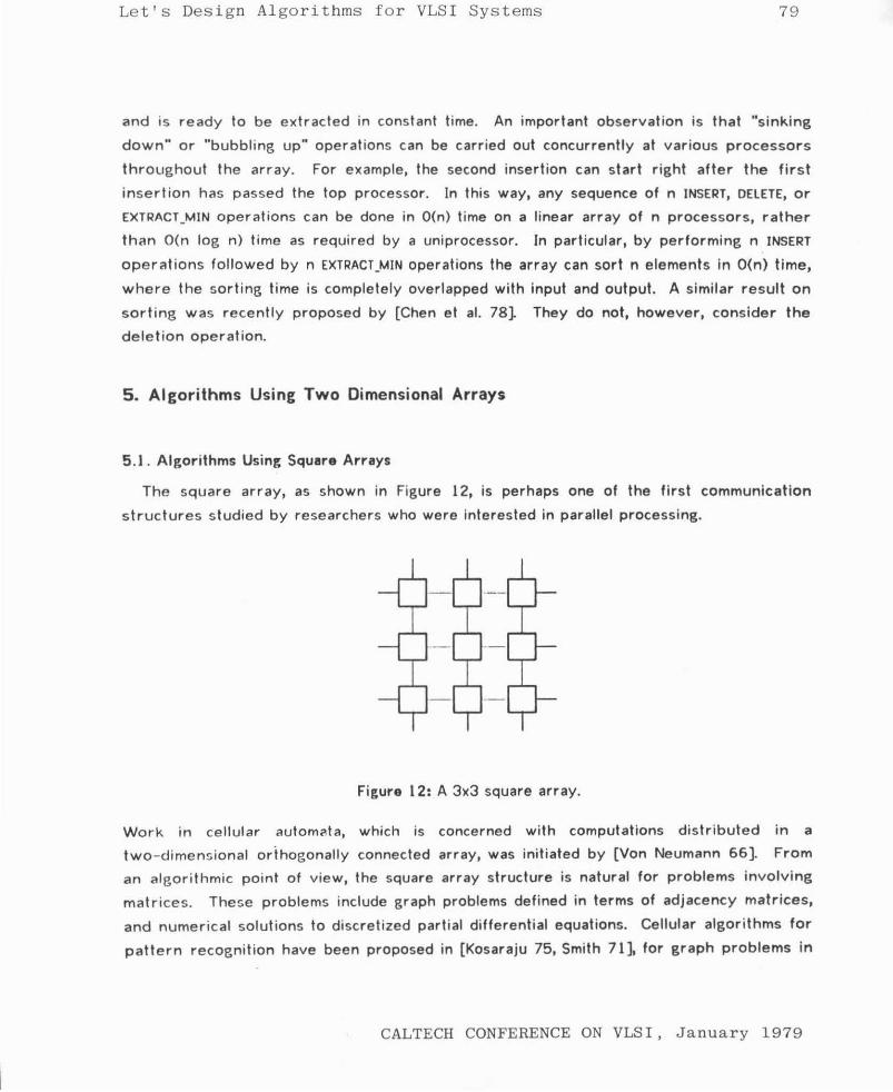
The square array, as shown in Figure 12, is perhaps one of the f irst communication

structures studied by researchers who were interested in parallel processing.

Figure 12: A 3x3 square array.

Work in cellular autom<'!ta, which is concerned with computations distributed in a

two- dimensional orthogonally connected array, was initiated by [Von Neumann 66). From

an algorithmic point of view, the square array structure is natural for problems involving

m at r ices. These problems include graph problems defined in terms of adjacency matrices,

and numerical solutions to discretized partial differential equations. Cellular algorithms for

pattern recognition have been proposed in [Kosaraju 75, Smith 71 ], for graph problems in


80 H. T. Kung

[Levitt and Kautz 72], for switching in [Kautz et al. 68], for sorting in [Thompson and Kung

77], and for dynamic programming in [Guibas et al. 79]. The algorithms for dynamic

programming in [Guibas et al. 79] are quite special in that they involve data being

transmitted at two different speeds, which give the effect of "time reverse" for the order

of certain results. For numerical problems, much of the research on the use of the square

structure is motivated or influenced by the ILLIAC IV computer, which has an 8x8

processor array. The broadcast capability provided by the ILLIAC IV is useful in

communicating relaxation and termination parameters required by many numerical methods.

This suggests that for VLSI implementation some additional broadcast facility be provided

on the top of the existing square array connection. This, however, would certainly

complicate the chip layout.

5.2. Algorithms Using Hexagonal Arrays

Figure 13: A 3x3 hexagonal array

The nexagonal array structure, as shown in Figure 13, enjoys the property of symmetry

in three directions. Therefore, after a binary operation is executed at a processor, the

result <~nd two inputs can all be sent to the neighboring processor in a completely

symmetric way. A good example is the matrix multiplication algorithm considered in Section

2, where elements in matrices A, B, and C all circulate throughout the network (cf. Figure

3). This type of computation eliminates a possible separate loading or unloading phase,

which is typically needed in algorithms using square array structures.

We know of two other problems that can be solved naturally on hexagonal arrays: LU

I NVITED SPEAKERS SESSION

Let's Desi gn Algorit hms for VLSI Systems 81

decomposi tion [Kung and Leiserson 78] and transitive closure [Guibas et al. 79]. We

indic ate below that, in some sense, these two problems and the matrix mult iplication

problem are all defined by recurrences of the "same" type. Thus, it is not coincidental that

they can be so lved b y similar algorithms using hexagonal arrays. The defining recurrences

for these problems are as follows:

Matrix Multi~lication

cO> I J 0,

(*) c{k+l) = I J c{k) + a·kbk ·

I J I J'

C" I J

c{f1+ 1) I J .

LU-decomposition

aO> I J = aij•

(*) a{f'-+1)= I J a{f'-) + l·k(-uk ·)

I J I J 1

{ !f~luk~ if i < k,

1ik if i ... k, if i > k,

ukj { ~k~) if k > j, if k ~ j.

Transitive Closure

a{k+l),.. I J

Notice that the main recurrences, denoted by (•), of the three problems have similar

structures for subscripts and superscripts.

CALTECH CONFERENCE ON VLSI , January 1979

82 H.T . Kung

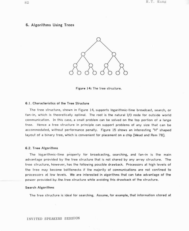
6. Algorithms Using Trees

Figure 14: The tree structure.

6.1 . Characteristics of the Tree Structure

The tree structure, shown in Figure 14, supports logarithmic-time broadcast, search, or

fan-in, which is theoretically optimal. The root is the natural 1/0 node for outside world

communication. In this case, a small problem can be solved on the top portion of a large

tree. Hence a tree structure in principle can support problems of any size that can be

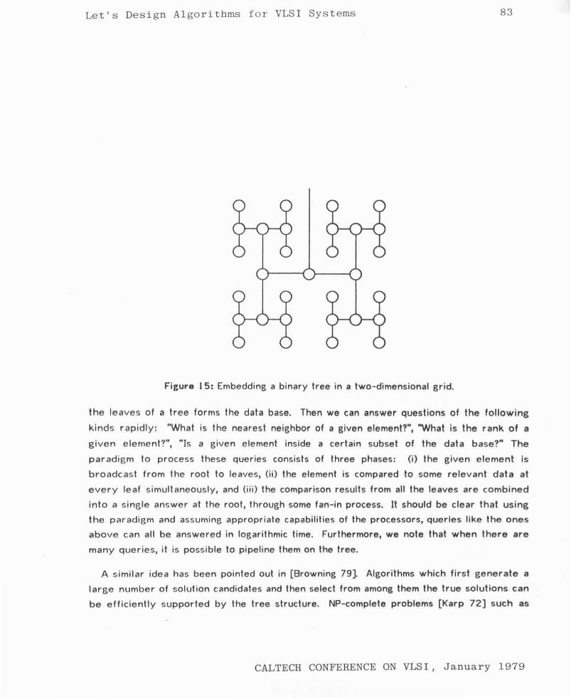
accommodated, without performance penalty. Figure 15 shows an interesting "H" shaped

layout of a binary tree, which is convenient for placement on a chip [Mead and Rem 78].

6.2. Tree Algorithms

The logarithmic-time property for broadcasting, searching, and fan-in is the main

advantage provided by the tree structure that is not shared by any array structure. The

tree structure, however, has the following possible drawback. Processors at high levels of

the tree may become bottlenecks if the majority of communications are not confined to

processors at low levels. We are interested in algorithms that can take advantage of the

pDwer provided by the tree structure_ while avoiding this drawback of the structure.

Search Algorithms

The tree structure is ideal for searching. Assume, for example, that information stored at


Let's Design Algor ithms for VLSI Systems 83

Figure 15: Embedding a binary tree in a two- dimensional grid.

the le aves of a tree forms the data base. Then we can answer questions of the following

kinds r apidly : "What is the nearest neighbor of a given element?", "What is the rank of a

given e le ment?", "Is a given element inside a certain subset of the data base?" The

paradig m to process these queries consi sts of three phases: (i) the given e lement is

broadcas t from the root to leaves, (ii) the element is compared to some relev ant data at

every leaf simultaneously , and (iii) the comparison results from all the leaves are combined

into a sing le answ er at the root, through some fan-in process. It should be clear that using

the p arad igm and assuming appropriate capabilities of the processors, queries like the ones

above can all be answered in logarithmic time. Furthermore, we note that when there are

many que r ies, it is possible to pipeline them on the tree.

A similar ide a has been pointed out in [Browning 79]. Algorithms which first generate a

large numbe r of solution candidates and then select from among them the true solutions can

be efficiently supported by the tree structure. NP-complete problems (Karp 72] such as


84 H.T . Kung

the clique problem and the color cost prooiem are solvable by such algorithms. One should

note that with this approach an exponential number of processors will be neecied to soive

an NP-complete problem in polynomial time. However, with the emergence of VLSI this

brute force approach may gain importance. Here we merely wish to point out that the tree

structure matches the structure of some algorithms that solve NP-complete problems.

Systolic Search Tree

As one is thinking about applications using trees, data structures such as search trees

(see, for example, [Aho et al. 75, Knuth 73)) will certainly come to mind. The problem is

how to embed a balanced search tree in a network of processors connected by a tree so

that the O(log n) performance for the INSERT, DELETE, and FIND operations can be maintained.

The problem is nontrivial because most balancing schemes require moving pointers around,

but the movement of pointers is impossible in a physical tree where pointers are fixed

wires. To get the effect of balancing in the physical tree, data rather than pointers must

be moved around. Common balanced tree schemes such as AVL trees and 2-3 trees do not

map well onto the tree network because data movements involved in balancing are highly

non-local. A new organization of a hardware search tree, called a systolic search tree, was

recently proposed by [Leiserson 79], on which the data movements for balancing are

always local so that the requirement of O(log n) performance can be satisfied. In

[Leiser son 79], an application of using the systolic search tree as a common storage for a

collection of disjoint priority queues is discussed.

Evaluation of Arithmetic Expressions and Recurrences

Another application of the tree structure is its use for evaluating arithmetic expressions.

Any expression of n variables can be evaluated by a tree of at most 4rlog2n 1 levels [Brent

74], but the time to input the n variables to the tree from the root is still O(n). This input

time can . often be overlapped with the computation time in the case of evaluating

recurrences. The idea of two-way pipeline algorithms for evaluating recurrences on linear

arrays (cf. Figure 11 (a)) extends directly to trees. Corresponding to the inner product

step processor in Figure 11 (b), for a tree we now have processors of the form shown in

Figure 16, which are def ined in terms of some given functions F, G1, and G2.

INVITED SPEAKERS SESSIO~

Let's Design Algorithms fo r VLSI Systems

y X

x, y

I y

2

X

x .- F (x 1, x

7, y)

Y, .- G,(x,, x7

, y)

Yz ._. ~(x,, xz, y)

Figure 16: The generalized inner product step processor for trees.

85

The tree structure can be used to evaluate systems of recurrences. The final vaiues of the

components of each term (which is a vector) are available at leaf processors, and are fed

back to the tree from the leaves for use in computing other terms. It is instructive to no'le

that all of the tree algorithms mentioned above correspond to various definitions of the

functions F, G11 and G2 at each processor (cf. Figure 16.)

7. Algorithms Using Shuffle-Exchange Networks

Consider a network having n=2m nodes, where m is an integer. Assume that nodes are

named 0, 1, ... , 2m-1. Let. imim-1 ... i1 denote the binary representation of any. integer I,

0 s i s 2m-1. The shuffle function is defined by

and the exchange function is defined by

The network is called a shuffle-exchange network if node i is connected to node S(l) for all

i, and to node E(i) for all even i. Figure 17 is a shuffle-exchange network of size n=8.

Observe that by using the exchange and shuffle connections alternately, data at pairs of

nodes whose names differ by 2i can be brought together for all i • 0, 1, ... , m-1. This

type of communication structure is common to a number of algorithms. It is shown in

[Satcher 68] that the bitonic sort of n elements could be carried out in O(log2 n) steps on

the shuffle-exchange network when the processing elements are capable of performing

comparison-exchange operations. It is shown in [Pease 68] that the n-point fast Fourier

CALTECH CONFERENCE ON VLSI, J a nuary 1979

86 H. T . Kung

0

7 0._

' 0

shuffle

6 2 exchange

Figure 17: A shuffle-exchange network.

transform could be done in O(log n) steps on the network when the processing elements

are capable of doing addition and multiplication operations. Other applications including

matrix transposition and linear recurrence evaluation are given in [Stone 71, Stone 75].

The two articles by Stone give clear expositions for all these algorithms and have good

discussions on the basic idea behind them.

Many powerful rearrangeable permutation networks, such as those in [Benes 65] which

are capable of performing all possible permutations in O(log n) delays, can be viewed as

multi - stage shuffle -exchange networks (see, e.g., (Kuck 78)). The shuffle-exchange

network, perhaps due to its great power in permutation, suffers from the fact that its

structure has a very low degree of regularity and modularity. This can be a serious

drawback, as far as VLSI implementations are concerned. Indeed, it was recently shown by

[Thompson 79] that the network is not planar and cannot be embedded in silicon using area

linearly proportional to the number of nodes.

8. Concluding Remarks

Many problems can be solved by algorithms that are "good" for VLSI implementation.

The communication geometries based on the array and tree structure or their combinations

seem to be sufficient for solving a large class of problems. When a large problem Is to be

solved on a small network, one can either decompose the problem or decompose an

algorithm that requires a large network [Kung 79].


Let's Des i gn Al go rithms fo r VLSI Systems 87

Algorithms employing multi-directional data flow can realize extremely complex

computations, without violating the simplicity and regularity constraints. Moreover, these

algorithms do not require separate loading or unloading phases. We believe that hexagonal

connection is fundamentally superior to square connection, because the former supports

data flows in more directions than the latter and the two structures are about of the same

complexity as far as implementations are concerned.

We need a new methodology for coping with the following problems:

- Notation for specifying geometry and data movements.

- Correctness of algorithms defined on networks.

- Guidelines for design of VLSI algorithms.

It is seen in this paper that there is a close relationship between the defining recurrence

of a problem and the VLSI algorithms for solving the problem. This association deserves

further research. We hope that eventually the derivation of good VLSI algorithms based on

given recurrences will be largely mechanical. An initial step towards this goal has been

independently taken by D. Cohen [Cohen 78).

ACKNOWLEDGMENTS

Comments by R. Hon, P. Lehman, S. Song, J. Bentley, C. Thompson and M. Foster at CMU

are appreciated.

References

[Aho et al. 75 ]

[Satcher 68]

[Benes 65]

[Brent 74]

Aho, A., Hopcroft, J.E. and Ullman, J.D.

The Design and Analysis of Computer Algorithms. Addison-Wesley, Reading, Massachusetts, 1975.

Satcher, K.E. Sorting networks and their applications. 1968 Spring Joint Computer Con f. 32:307-314, 1968.

Benes, V.E. Mathematical Theory of Connecting Networks and Telephone Traffic. Academic Press, New York, 1965.

Brent , R.P. The Parallel Evaluation of General Arithmetic Expressions. Journal of the ACM 21(2):201-206, April 1974.

CALTECH CONFERENCE ON VLSI , January 1979

88

[Browning 79]

H.T. Kung

Browning, S. Algorithms for the Tree Machine.

To appear in the forthcoming book, Introduction to VLSI Systems, by C. A. Mead and L.A. Conway, Addison-Wesley.

[Chen 75] Chen, T.C. Overlap and Pipeline Processing, pages 375-431. In Introduction to Computer Architecture, (Stone, H.S., Editor), Science

Research Associates, 1975.

[Chen et al. 78) Chen, T.C., Lum, V.Y. and Tung, C. The Rebound Sorter: An Efficient Sort Engine for Large Files Proceedings of the 4th International Conference on Very Large Data

Bases, IEEE, pages 312-318, 1978.

[Cohen 78] Cohen, D. Mathematical Approach to Computational Networks. Technical Report ISI/RR-78-73, University of Southern California,

Information Sciences Institute, November 1978.

[Guibas et al. 79] Guibas, L.J., Kung, H.T. and Thompson, C.D. Direct VLSI Implementation. of CombinatoriaL Algorithms Proc. Conference on Very Large Scale Integration: Architecture, Design,

Fabrication, California Institute of Technology, January, 1979.

(Hallin and Flynn 72) Hallin, T.G. and Flynn, M.J. Pipclining of Arithmetic Functions. I£££ Trans. on. Comp. C-21 :880-886, 1972.

[Karp 72 ] Karp, R. M. Reducibility Among Combinational Problems, pages 85-104. In Complexity of Computer Computations, Plenum Press, New York,

1972.

(Kautz e t al. 68] Kautz, W.H., Levi tt, K.N. and Waksman, A. Cellular Interconnection Arrays. I£££ Transactions on Computers C- 17(5):443- 451, May 1968.

(Knuth 73) Knuth, D. E. The Art o f Computer Programming. Volume 3: Sorting and Searching. Addison-Wesley, 1973.

[Kosaraju 75) Kosaraju, S.R. Speed of Recognition of Context-Free Languages by Array Automata. S IAM ). on. Computing 4:33 1-340, 1975.

[Kuck 78) Kuck, D. J. The Structure of Computers and Computations. John Wiley and Sons, New York, 1978.

[Kung 79) Kung, H. T.


Let 's Design Algo r it hms £or VLS I Sys~ems 89

The Structure of Parallel Algorithms. In Advances in Computers, (Yovits, M. C., Editor), Academic Press, New

York, 1979.

[Kung and Lciserson 78]

[Leiserson 79]

Kung, H. T. and Leiserson, C. E. Systolic Arrays (for VLS[). Technical Report, Carnegie-Mellon University, Department of Computer

Science, December 1978. To appear in the forthcoming book, introduction to VLSI Systems, by

C. A. Mead and L. A. Conway, Addison-Wesley, 1979.

Leiserson, C. E. Systolic Priority Queues Proc. Conference on Very Large Scale Integration: Architecture, Design,

Fabrication, California Institute of Technology, January, 1979.

[Levitt and Kautz 72] Levitt, K.N. and Kautz, W.H. Cellular Arrays for the Solution of Graph Problems. Communications of the ACM 15(9):789-801, September 1972.

[Mead and Conway 79] Mead, C. A. and Conway, L. A. Introduction to VLSI Systems. Addison- Wesley, 1979.

[Mead and Rem 78]

[Pease 68)

Mead, C. and Rem, M. Cost and Performance of VLSI Computing Structures. Technical Report 1584, California Institute of Technology, Department of

Computer Science, 1978.

Pease, M.C. An Adaptation of the F?st Fourier Transform for Parallel Proce~sing. Journal of the ACM 15:252-264, April 1968.

[Ramamoorthy and Li 77)

[Smith 7 1]

[Stone 71]

Ramamoorthy, C.V. and Li, H.F. Pipeline Architecture. Computing Surveys 9(1}:61-102, March 1977.

Smith III, A.R. Two-Dimensional Pormal Languages and Pattern Recognition by Cell.u.la.r

Automata 12th IEEE Symposium on Switching and Automata Theory, pages

144-152, 1971.

Stone, H.S. Parallel Processing with the Perfect Shuffle. IE££ Transactions on Computers C-20:153-161, February 1971.

CALTECH CONFERENCE ON VLS I, January 1979

90

[Stone 75] Stone, H.S.

Parallel Computation, pages 318-37 4. In Introduction to Computer Architecture, (Stone, H.S., Editor), Science

Research Associate, Chicago, 1975.

[Sutherland and Mead 77] Sutherland, I. E. and Mead, C. A. Microelectronics and Computer Science. Scientific American 237:210-228, 1977.

[Thompson and Kung 77]

[Thompson 79]

Thompson, C.O. and Kung, H.T. Sorting on a Mesh-Connected Parallel Computer. Communications of the ACM 20(4):263-271, April 1977.

Thompson, C.O. Area-Time Complexity for VLSI Eleventh Annual ACM Symposium on Theory of Computing, May, 1979.

[Von Neumann 66] Von Neumann, J. Theory of Self-Reproducing Automata. (Burks, A. W., Editor), University of Illinois Press, Urbana, Illinois, 1966.


Documents

Let's Design Algorithms for VLSI Systems - …caltechconf.library.caltech.edu/192/1/HTKung.pdfLet's Design Algorithms for VLSI Systems H. T. Kung Department of Computer Science Carnegie-Mellon