Embed Size (px)
Citation preview
Invent math (2010) 182: 231–277DOI 10.1007/s00222-010-0262-y
Length spectra and degeneration of flat metrics
Moon Duchin · Christopher J. Leininger ·Kasra Rafi
Received: 21 July 2009 / Accepted: 25 May 2010 / Published online: 9 June 2010© Springer-Verlag 2010
Abstract In this paper we consider flat metrics (semi-translation structures)on surfaces of finite type. There are two main results. The first is a completedescription of when a set of simple closed curves is spectrally rigid, that is,when the length vector determines a metric among the class of flat metrics.Secondly, we give an embedding into the space of geodesic currents and usethis to obtain a compactification for the space of flat metrics. The geometricinterpretation is that flat metrics degenerate to mixed structures on the surface:part flat metric and part measured foliation.
The first author is partially supported by NSF grant DMS-0906086. The second author ispartially supported by NSF grant DMS-0905748.
M. Duchin (�)Department of Mathematics, University of Michigan, 530 Church Street, Ann Arbor,MI 48109-1043, USAe-mail: [email protected]: http://www.math.lsa.umich.edu/~mduchin
C.J. LeiningerDepartment of Mathematics, University of Illinois at Urbana-Champaign, 1409 W. GreenSt., Urbana, IL 61801, USAe-mail: [email protected]: http://www.math.uiuc.edu/~clein/
K. RafiDepartment of Mathematics, University of Oklahoma, Norman, OK 73019-0315, USAe-mail: [email protected]: http://www.math.ou.edu/~rafi/

232 M. Duchin et al.
1 Introduction
From the lengths of all, or some, curves on a surface S, can you identifythe metric? To be precise, fix a finite-type surface S, denote by C(S) the setof homotopy classes of closed curves on S, and let S(S) be the homotopyclasses represented by simple closed curves (simply denoted by C and S whenS is understood). Given an isotopy class of metrics ρ and a curve α ∈ C,we write �ρ(α) to denote the infimum of lengths of representatives of α ina representative metric for ρ, and we call this the length of α in ρ or theρ-length of α. For a set of curves � ⊂ C, we define the (marked) �-lengthspectrum of ρ to be the length vector, indexed over �:
λ�(ρ) = (�ρ(α))α∈� ∈ R�.
For a family of metrics G = G(S), up to isotopy, and a family of curves �,we are interested in the problem of deciding when λ�(ρ) determines ρ. Inother words, we ask
Question Is the map G → R� given by ρ �→ λ�(ρ) an injection?
If this map is injective, so that ρ ∈ G is determined by the lengths of thecurves in �, we say that � is spectrally rigid over G .
For instance, we may take � = S, and G = T (S), the Teichmüller space ofcomplete finite-area hyperbolic (constant curvature −1) metrics on S. Here itis a classical fact due to Fricke that the map T (S) → R
S is injective; that is,S is spectrally rigid over T (S).
Another natural family of metrics arising in Teichmüller theory consistsof those induced by unit-norm quadratic differentials; these are locally flat(isometrically Euclidean) away from a finite number of singular points withcone angles kπ . We note that these are nonpositively curved in the sense ofcomparison geometry, though they fail to be complete when S has punctures.We will call these flat metrics on S (see Sect. 2 for a detailed discussion). Forexample, identifying opposite sides of a regular Euclidean octagon producesa flat metric on a genus-two surface, with the negative curvature concentratedinto one cone point of angle 6π . We denote this family of metrics by Flat(S).
Theorem 1 For any finite-type surface S, the set of simple closed curves S isspectrally rigid over Flat(S).
Put in other terms, this theorem states that the lengths of simple closedcurves determine a quadratic differential up to rotation.
In fact, we obtain a much sharper version of Theorem 1 which provides acomplete answer to the motivating question above for simple closed curvesover flat metrics. Let P M F = P M F (S) denote Thurston’s space of projec-
Length spectra and degeneration of flat metrics 233
tive measured foliations on S. We use ξ = ξ(S) = 3g − 3 + n, where g is thegenus and n is the number of punctures, as a measure of complexity for S.
Theorem 2 If ξ(S) ≥ 2, then � ⊂ S ⊂ P M F is spectrally rigid over Flat(S)
if and only if � is dense in P M F .
This situation is quite different from the hyperbolic case, where there arefinite spectrally rigid sets for T (S), as is further discussed in Sect. 1.1. Wealso remark that if ξ(S) ≤ 1 then it is easy to see that any set of three distinct,primitive curves is spectrally rigid over Flat(S); see Proposition 17.
One direction of the proof of Theorem 2 requires us to construct flat struc-tures which cannot be distinguished by the lengths of the curves in �. Infact, we produce subspaces of Flat(S) with dimension approximately linearin dim(Flat(S)) = 4ξ −2 on which the lengths of the curves in � are constant.
Theorem 3 Suppose ξ(S) ≥ 2. If � ⊂ S ⊂ P M F and � �= P M F , thenthere is a deformation family � ⊂ Flat(S) for which � → R
� is constant,and such that the dimension of � grows linearly with ξ(S), as does thedimension of Flat(S) itself.
In particular, in the closed case, our construction produces a subspace� ⊂ Flat(S) of dimension 2g − 3, while the dimension of Flat(S) in thiscase is 12g − 14.
Another result needed for the proof of Theorem 2 is a version of Thurston’stheorem that the hyperbolic length function for simple closed curves contin-uously extends to the space M F (S) of measured foliations (or laminations)on S. In [4], Bonahon gave a very elegant proof of this for closed surfacesbased on a unified approach to studying hyperbolic metrics, closed curvesand laminations. Bonahon’s key idea is to embed C(S), T (S) and M F (S),into the space of geodesic currents C(S). Our next result extends the theoryto flat structures.
Theorem 4 There is an embedding
Flat(S) → C(S)
denoted by q �→ Lq so that for q ∈ Flat(S) and α ∈ C, we have i(Lq,α) =�q(α). Furthermore, after projectivizing, Flat(S) → P C(S) is still an embed-ding.
As a consequence, we obtain a continuous homogeneous extension of theflat length function in Corollary 28,
Flat(S) × M F (S) → R,
making it meaningful to discuss the length of a foliation.

234 M. Duchin et al.
As P C(S) is compact, Theorem 4 provides a compactification of Flat(S),and it is invariant under the action of the mapping class group. Bonahonproved that for closed surfaces, the analogous compactification of T (S) isprecisely the Thurston compactification by projective measured laminations.For the compactification of Flat(S), we also find a geometric interpretation ofthe boundary points as mixed structures on S. A mixed structure is a hybridof a flat structure on a subsurface (with boundary length zero) and a mea-sured lamination on the complementary subsurface. (The reader should com-pare our mixed structures to forthcoming work of Cooper, Delp, Long andThistletwhaite, whose geometric description of degeneration in the setting ofreal projective structures inspired this interpretation of the limit points.) Weview the space of mixed structures as a subspace of C(S), and thus for anymixed structure η, there is a well-defined intersection number i(η, ·). Thistheory is developed in Sect. 6.
Theorem 5 The closure of Flat(S) in P C(S) is exactly the space P Mix(S) ofprojective mixed structures. That is, for any sequence {qn} in Flat(S), afterpassing to a subsequence if necessary, there exists a mixed structure η and asequence of positive real numbers {tn} so that
limn→∞ tn�qn(α) = i(α, η).
for every α ∈ C. Moreover, every mixed structure is the limit of a sequence inFlat(S).
In Sects. 6 and 7 we make several other comparisons between this com-pactification and the Thurston compactification of T (S).
Remark 6 For the purpose of geodesic currents, punctured surfaces are con-sidered as surfaces with holes; this is treated carefully in Sect. 2.6. Thisrequires new definitions and makes the machinery of currents considerablymore technical. The results on spectral rigidity (Theorems 1–4) can be provedfor closed surfaces without using these definitions, but punctured surfaces areunavoidable for the characterization of the boundary in Theorem 5, since theboundary points even for closed surfaces involve currents on punctured sub-surfaces. To read the spectral rigidity part of the paper for closed surfacesalone, one would skip Sects. 2.6, 6, 7.2, and the Appendix.
1.1 Context: other spectral rigidity results
Spectral rigidity of S over T (S) was generalized considerably by Otal [24],who showed that C is spectrally rigid over G−(S), the space of all negativelycurved metrics on S up to isotopy. Hersonsky-Paulin [16] generalized this
Length spectra and degeneration of flat metrics 235
further to show that C is spectrally rigid over negatively curved cone metrics.This was pushed in a different direction by Croke [8], Fathi [10] and Croke-Fathi-Feldman [7] where it was shown that C is spectrally rigid for variousqualities of nonpositively curved Riemannian metrics (for more precise state-ments, see the references).
While these results treat rather large classes of metrics, the use of all closedcurves, not just the simple ones, is essential. Indeed, it follows from a resultof Birman-Series [2] that, in general, we should not expect S to be spectrallyrigid for an arbitrary class of negatively curved metrics, since simple closedcurves miss most of the surface (see Sect. 7).
We saw above in Theorem 2 that a set of curves must be dense in thesphere P M F in order to be spectrally rigid over Flat(S). This stands in con-trast with the situation for hyperbolic metrics, where it is known that there arefinite spectrally rigid sets; in fact, 2ξ + 1 curves, one more than the dimen-sion of T (S), are sufficient (see [14, 15, 28]). In this regard, Flat(S) bearsa resemblance to Outer space, CV(Fn). The Culler–Vogtmann Outer space,built to study the group Out(Fn) in analogy to the relationship between T (S)
and the mapping class group, consists of metric graphs X equipped with aisomorphisms Fn → π1(X) (under the equivalence relation of graph isome-tries which respect the isomorphism up to conjugacy). Recycling notationsuggestively, let C denote the set of conjugacy classes of nontrivial elementsof Fn. Given an element X ∈ CV(Fn), and a conjugacy class α ∈ C, we write�X(α) for the minimal-length representative of α in X. We can define a lengthspectrum just as above, letting
λ�(X) = (�X(α))α∈� ∈ R�
for X ∈ CV(Fn) and � ⊂ C. Accordingly, we say that � is spectrally rigidover CV(Fn) if X �→ λ�(X) is injective.
The full set C is spectrally rigid over CV(Fn) [1, 9]. However, Smillie andVogtmann (expanding on a similar result of Cohen, Lustig and Steiner [6])showed that no finite subset � ⊂ C is spectrally rigid over Outer space (oreven the reduced Outer space) by finding a (2n − 5)-parameter family ofgraphs over which λ� is constant [29]. Thus, Theorem 3 is the analog forFlat(S) of the Smillie–Vogtmann result. Our proof of Theorem 3 adapts thekey idea from Smillie–Vogtmann to surfaces by appealing to Thurston’s the-ory of train tracks; see Sect. 4. This justifies the remark that from the point ofview of length-spectral rigidity, flat metrics might be said to resemble metricgraphs more closely than hyperbolic metrics.
Finally, we briefly consider unmarked inverse spectral problems for themetrics in Flat(S). Kac memorably asked in 1966 whether one can “hear theshape of a drum,” or determine a planar region by the eigenvalues of its Lapla-cian. Sunada’s work in the 1980s established a means of generating examples

236 M. Duchin et al.
of hyperbolic surfaces which are not only isospectral with respect to theirLaplacians, but iso-length-spectral as well. That is, let the unmarked lengthspectrum be the nondecreasing sequence of numbers
�C(ρ) = {�ρ(γ1) ≤ �ρ(γ2) ≤ · · · }γi∈C,
appearing as lengths of closed curves on S, listed with multiplicity. Sunada’sconstruction produces a supply of examples of hyperbolic metrics m,m′ suchthat �C(m) = �C(m′). In Sect. 7.3, we remark that the Sunada constructioncarries over to our flat metrics in the same way.
2 Preliminaries: flat structures, foliations, and geodesic currents
In this section, we will briefly describe the background and preliminary mate-rial on Teichmüller theory, semi-translation surfaces, flat metrics, Thurston’stheory of projective measured foliations, and Bonahon’s theory of geodesiccurrents. We refer the reader to [3, 4, 11, 12, 25, 30].
In what follows, S is a finite-type surface. That is, S is obtained from aclosed surface S by removing a finite set P ⊂ S of marked points. The genusg and number of punctures n = |P | determine the topological complexity
ξ = ξ(S) = 3g − 3 + n.
Recall that Teichmüller space T (S), which parameterizes the isotopy classesof hyperbolic metrics on S, is homeomorphic to a ball of dimension 2ξ .
2.1 Quadratic differentials and semi-translation structures
By a quadratic differential on S we mean a complex structure on S togetherwith an integrable meromorphic quadratic differential. The quadratic differ-ential is allowed to have poles of degree one at marked points and is assumedto be holomorphic on S. The space of all quadratic differentials, defined upto isotopy, is denoted Q(S). A point of Q(S) will be denoted q , with the un-derlying complex structure implicit in the notation. Reading off the complexstructures, we obtain a projection to the Teichmüller space
π : Q(S) → T (S).
This projection is canonically identified with the cotangent bundle to T (S);hence Q(S) has a real dimension of 4ξ .
Integrating the square root of a nonzero quadratic differential q in a smallneighborhood of a point where q is nonzero produces natural coordinates ζ
on S in which q = dζ 2. The collection of all natural coordinates gives an atlas
Length spectra and degeneration of flat metrics 237
on the complement of the zeros of q for which the transition functions aregiven by maps of the form z �→ ±z + c for c ∈ C (called semi-translations).The Euclidean metric is preserved by these transition functions and so pullsback to a Euclidean metric on the complement of the zeros of q in S. Theintegrability of q implies that the metric has finite total area.
The completion of the metric is obtained by replacing the zeros of q as wellas the points P to obtain the surface S. If q has a zero of order p at one of thecompletion points, then there is a cone singularity with cone angle (2 + p)π .A pole at a point of P is thought of as a zero of order −1, and hence has coneangle π . Thus the metric on S is locally CAT(0) (or nonpositively curved inthe sense of comparison geometry)—however, the metric on S may not be,because of the discrete positive curvature occurring at poles. We also use q todenote the completed metric on S.
A semi-translation structure is a locally CAT(0) Euclidean cone metric onS, whose completion is S, together with a maximal atlas defining the met-ric away from the cone points, for which the transition functions are semi-translations. The atlas determines a preferred vertical direction, and the met-ric together with the vertical direction determines the semi-translation struc-ture. Given a semi-translation structure, there is a unique complex structureand integrable holomorphic quadratic differential for which the charts in theatlas are natural coordinates. This determines a bijection between the set ofnonzero quadratic differentials and the set of semi-translation structures on S,which we use to identify the two spaces. The Teichmüller metric is inducedby the co-norm on Q(S) which comes from the area of the associated semi-translation structure on S. The unit cotangent space, Q1(S), is thus preciselythe set of unit-area semi-translation structures on S.
A semi-translation structure can also be described combinatorially as a col-lection of (possibly punctured) polygons in the Euclidean plane with sidesidentified in pairs by gluing isometries that are the restrictions of semi-translations.
The group SL2(R) acts naturally on the space of quadratic differentialsby R-linear transformation on the natural coordinates. The geodesics in theTeichmüller metric are precisely projections to T (S) of orbits of the diagonalsubgroup of SL2(R) on an initial quadratic differential q0:
γ (t) ={π(At .q0) : At =
(et 00 e−t
), t ∈ R
}.
The Teichmüller disk Hq of a quadratic differential q is the projection to T (S)
of its entire SL2(R) orbit; it is an isometrically embedded copy of the hyper-bolic plane of curvature −4.
We let p : S → S denote the universal covering of S, with π1(S) actingby covering transformations. The metric q pulls back to a metric q = p∗(q)

238 M. Duchin et al.
on S which is again locally CAT(0). When S is a closed surface, (S, q) is acomplete, geodesic CAT(0) space. If S has punctures, then (S, q) is incom-plete, and we write (S, q) for the completion, obtaining a geodesic CAT(0)
space. The covering p : S → S can be extended to the completions which wealso denote by p. This extension can be viewed as a branched cover, infinitelybranched over P , and we let P denote the preimage of P in S.
Example 7 Consider again the unit-area regular octagon (with opposite sidesidentified and one pair of sides parallel to the vertical direction) as a pointQ1(S), for S the closed surface of genus two. The universal cover is madeup of isometric copies of the octagon, glued together with eight around eachvertex to create cone points of angle 6π . This metric q on S is a discretemodel of the hyperbolic plane (it is quasi-isometric to H), and with this metricS has a circle as its boundary at infinity.
2.2 Measured foliations and measured laminations
We now recall Thurston’s theory of singular topological foliations of surfaces,equipped with transverse measures; see [11] for a detailed discussion andreference for the facts stated here. We write M F = M F (S) for the spaceof (measure classes of) measured foliations on S, and P M F = P M F (S)
to denote the space of projective measured foliations. Thurston showed thatP M F (S) is a sphere, and used it to compactify the Teichmüller space.A curve α ∈ S canonically determines a measured foliation with all nonsin-gular leaves closed and homotopic to α. We use this to view R+ × S and S assubsets of M F and P M F , respectively. The image of S in P M F is dense,so P M F may be thought of as a completion of the set of simple closedcurves.
We also write
i : M F × M F → R
for Thurston’s geometric intersection number. This is the unique homoge-neous continuous extension of the usual geometric intersection number onS × S, via the inclusion mentioned above.
The vertical foliation for a nonzero quadratic differential q ∈ Q(S) is givenby |Re(
√q)|. Let νθ
q be the foliation |Re(eiθ√q)| for θ ∈ RP1, so that thevertical foliation of q is νq := ν0
q . By setting
M F (q) := {t · νθq : θ ∈ RP1, t ∈ R+},
we obtain the set of all measured foliations which are straight in some direc-tion on q , with measure proportional to Euclidean distance between leaves.We write P M F (q) for the projectivization of M F (q).
Length spectra and degeneration of flat metrics 239
It will be useful to pass back and forth between measured foliations andmeasured laminations. We denote the space of measured laminations by M Land the projective measured laminations by P M L. We identify M F withM L and P M F with P M L in the natural way extending the canonical in-clusions of S. See [19] for an explicit procedure for constructing laminationsfrom foliations.
2.3 The space of flat metrics
Quadratic differentials that represent the same metric differ only by a rotation.Accordingly, the space of flat metrics is defined as
Flat(S) = Q1(S)/q ∼ eiθq.
Equivalently, an element of Flat(S) is a Euclidean cone metric on S which islocally CAT(0), with holonomy in {±I }, completion S, and total area one.This is almost identical to the notion of a quadratic differential, but there isone forgotten piece of data, namely the preferred vertical direction which isdetermined by the atlas of natural coordinates. We write q to denote a pointin Q1(S) or the associated equivalence class in Flat(S). Note that M F (q)
and P M F (q) are well-defined for q ∈ Flat(S). Also, each Teichmüller diskHq lifts to an embedded disk in Flat(S), and in fact, Flat(S) is foliated byTeichmüller disks.
2.4 Geodesics
Let q be a quadratic differential on S and (S, q) the completion of the pull-back metric q on S. Every curve α ∈ C has a q-geodesic representative in thefollowing sense: for a map α : S1 → S from the unit circle to S, there is anisometric map αq : R → (S, q) (i.e., a geodesic of S) such that a subgroup ofπ1(S) corresponding to the curve α preserves the image αq(R). The projec-tion of this to S is the q-geodesic representative of α and we denote it by αq .(This definition seems cumbersome, but when P �= ∅ the map αq alone doesnot determine the homotopy class α, whereas αq does. See [27] for moredetails.) We call the q-geodesic αq , or any π1(S)-translate of it, a lift of αq .
To describe geodesics concretely, it will be useful to define saddle con-nections: these are geodesic segments whose endpoints are (not necessarilydistinct) singularities or points of P , and which have no singularities or pointsof P in their interiors.
Remark 8 We make an elementary but very useful observation that identifiesthe geodesics in a flat metric q . First consider the case that S is closed. Given arepresentative of α built as a concatenation of saddle connections α1 · · ·αk , a

240 M. Duchin et al.
necessary and sufficient condition for this to be a q-geodesic is that the anglesbetween successive αi measure at least π on both sides. When P is nonempty,we need to modify this slightly. Suppose α1 · · ·αk is a representative of α inS and consider a lift of this representative to S; that is, α1 · · ·αk is a limit ofrepresentatives of α in S and the lift is a limit of lifts. Then we require that anangle of at least π is subtended at each point in P as well. (Note that pointsof P are locally modeled on the infinite cyclic branched cover of the plane,branched over the origin, so there is exactly one finite angle at each such pointmet by the lift.)
The geodesic representative of α is unique (up to parameterization), ex-cept when there are a family of parallel geodesic representatives foliating aflat cylinder. We also note that the geodesic representative of a simple closedcurve need not be simple. However, for every curve α, there is always a se-quence of representatives of the homotopy class of α in S converging uni-formly to αq .
When S is a punctured surface, we will also be interested in homotopyclasses of essential proper paths in S. These are paths α : I → S, defined onsome closed interval I , for which the interior of I is mapped to S and theendpoints are mapped to P . Here, two such paths are homotopic if there isa homotopy relative to the endpoints so that throughout the homotopy theinterior of I is mapped to S. We denote the set of all homotopy classes ofessential curves and paths by C′(S), which is equal to C(S) if S is closed.Every element of C′(S) has a unique geodesic representative, which we viewas the projection of an isometric embedding αq : I → (S, q) to S, and isagain denoted by αq . Again, αq is a uniform limit of representatives of thehomotopy class of α.
When a curve α has non-unique geodesic representatives that foliate acylinder, we say α is a cylinder curve and we define the cylinder set of q ,denoted by cyl(q), to be the set of all cylinder curves with respect to q .
When α ∈ C′(S) is not a cylinder curve, the (unique) geodesic representa-tive is made up of concatenations of saddle connections. (In fact, each bound-ary component of a cylinder is a union of saddle connections, so even cylindercurves have representatives of this form.) If we write this concatenation as
αq = α1 · · ·αk,
and let rj denote the Euclidean length of αj , then �q(α) is just r1 + · · · + rk .If we view q as a quadratic differential (and not just as a flat structure),
then each αj makes some angle θj with the horizontal direction.
Lemma 9 For all q ∈ Q1(S) and α ∈ C′(S), we have
�q(α) = 1
2
∫ π
0i(νθ
q , α)dθ.
Length spectra and degeneration of flat metrics 241
Proof This is a computation:
∫ π
0i(νθ
q , α) dθ =∫ π
0
(k∑
j=1
∫αj
|Re(eiθ√q )|)
dθ
=k∑
j=1
∫ π
0rj | cos(θ + θj )|dθ =
k∑j=1
2rj = 2�q(α).�
While the q-geodesics αq and βq are not necessarily embedded or trans-verse, they do meet minimally in a certain sense. Namely, appealing to theCAT(0) structure, we first note that any two lifts αq and βq meet in a point, ina geodesic segment, or they are disjoint. If the endpoints at infinity of αq andβq nontrivially link, then we call these intersections essential intersections.It follows that i(α,β) is the number of π1(S)-orbits of essential intersectionsover all lifts of αq and βq .
2.5 Geodesic currents: closed surfaces
The theory of geodesic currents was initiated in a sequence of papers byBonahon and an excellent overview can be found in [4]. For this discussion,we first restrict to the closed case (P = ∅), which is the case treated by Bona-hon in [4].
Fix any geodesic metric g on S. We can pull back this metric by the univer-sal covering p : S → S, so that the covering group action of π1(S) on S is byisometries. We let S∞ denote the Gromov boundary of S, making S ∪ S∞ intoa closed disk. This compactification is independent of the choice of metric (inthe sense that a different choice of metric gives an alternate compactificationfor which the identity extends to a homeomorphism of the boundary circles).
We consider the space
G(S) = (S∞ × S∞ \ �)/(x, y) ∼ (y, x).
With respect to our metric, this is precisely the space of unoriented bi-infinitegeodesics in S up to bounded Hausdorff distance. We endow G(S) with thediagonal action of π1(S).
A geodesic current on S is a π1(S)-invariant Radon measure on G(S). Theset of all geodesic currents is made into a (metrizable) topological space byimposing the weak* topology, and we denote this space C(S). The associatedspace of projective currents is the quotient of the space of nonzero currentsby positive real scalar multiplication, and we denote it P C(S).
The simplest examples of geodesic currents are defined by closed curvesα ∈ C as follows. Given such a curve α, we first realize it by a geodesic

242 M. Duchin et al.
representative (with respect to our fixed metric). The preimage p−1(α) inS determines a discrete subset of G(S) (independent of the metric), and tothis we can associate a Dirac measure on G(S), for which π1(S)-invariancefollows from the invariance of p−1(α). This injects the set C into C(S), andwe will thus view C as a subset of C(S) when convenient. While these arevery special types of geodesic currents, the set of positive real multiples of allcurves is in fact dense in C(S), as shown in [4].
In [3], Bonahon constructs a continuous extension for the geometric inter-section number to all currents.
Theorem 10 (Bonahon) The geometric intersection number i : C(S) ×C(S) → R has a continuous, bilinear extension
i : C(S) × C(S) → R.
Moreover, in [24], Otal proved that i and C can be used to separate points:
Theorem 11 (Otal) Given μ1,μ2 ∈ C(S), μ1 = μ2 if and only if i(μ1, α) =i(μ2, α) for all α ∈ C.
From this, one can easily deduce a convergence criterion and also define ametric on the space of currents which will be convenient for our purposes.
Theorem 12 A sequence μk ∈ C(S) converges to μ ∈ C(S) if and only if
limk→∞ i(μk,α) = i(μ,α)
for all α ∈ C. Furthermore, there exist tα ∈ R+ for each α ∈ C so that
d(μ1,μ2) =∑α∈C
tα∣∣ i(μ1, α) − i(μ2, α)
∣∣
defines a proper metric on C(S) which is compatible with the weak* topology.
Before we prove this theorem, we recall one further fact due to Bonahon[4] which we will need. We say that a geodesic current ν is binding if forevery (x, y) ∈ G(S), there is an (x′, y′) in the support of ν such that (x, y)
and (x′, y′) link in S∞. With respect to any fixed metric, this is equivalent torequiring that every bi-infinite geodesic in S intersects some geodesic in thesupport of ν. It follows, as discussed by Bonahon, that any binding currentand any nonzero current have positive intersection number. As an example,any filling curve or union of curves determines a binding current.

Length spectra and degeneration of flat metrics 243
Proposition 13 (Bonahon) If ν is a binding geodesic current and R > 0, thenthe set
{μ ∈ C(S) | i(μ, ν) ≤ R}is a compact set. Consequently, the set
{μ
i(μ, ν)
∣∣∣μ ∈ C(S) \ {0}}
is compact, and hence so is P C(S).
Proof of Theorem 12 Continuity of i implies i(μk,α) → i(μ,α) for all α ∈ C
if μk → μ. To prove the other direction, assume i(μk,α) → i(μ,α) for allα ∈ C. In particular, if we let α0 ∈ C be a filling curve (so the associatedcurrent is binding), then i(μk,α0), i(μ,α0) ≤ R for some R > 0. So, {μk} ∪{μ} is contained in some compact set by Proposition 13.
Since C(S) is metrizable, it follows that there is a convergent subsequenceμkn → μ′ for some μ′ ∈ C(S). Continuity of i implies that i(μ,α) = i(μ′, α)
for all α, and so Theorem 11 guarantees that μ = μ′. Since this is true for anyconvergent subsequence of {μk} it follows that μk → μ. This completes theproof of the first statement of the theorem.
To build the metric we must first find the numbers {tα}. For this, we observethat for any μ ∈ C(S) and fixed choice of a filling curve α0, the numbers
{i(μ,α)
i(α0, α)
}α∈C
={
i
(μ,
α
i(α0, α)
)}α∈C
are uniformly bounded. This follows from the fact that the set of currents
{α
i(α0, α)
}α∈C
is precompact by Proposition 13.Now we enumerate all closed curves α0, α1, α2, . . . ∈ C (α0 still denoting
our filling curve). Set tk = tαk= 1/(2k i(α0, αk)). It follows that
∞∑k=0
tk i(μ,αk) =∞∑
k=0
1
2ki
(μ,
αk
i(α0, αk)
)
converges and hence the series for d given in the statement of the propositionconverges. Symmetry and the triangle inequality are immediate, and positivityfollows from Theorem 11. The fact that the topology agrees with the weak*topology is a consequence of the first part of the Theorem and the fact that

244 M. Duchin et al.
C(S) is metrizable (hence first countable, so determined by its convergentsequences).
Finally, we verify that the metric is proper. Proposition 13 implies that forany binding current ν ∈ C(S), the set
A ={
μ
i(μ, ν)
∣∣∣μ ∈ C(S) \ {0}}
is compact. Since d is continuous, the distance from 0 to any point of A isbounded above by some R > 0 and below by some r > 0. Furthermore, forany μ ∈ C(S) and t ∈ R+, we have
d(tμ,0) = t · d(μ,0).
Hence, the compact set
A′ = {tμ |μ ∈ A, t ∈ [0,1]}is contained in the ball of radius R and contains the ball of radius r . Fromthis and the preceding equation, it follows that for any ρ > 0, the closed ballof radius ρ > 0 about 0 is a compact set. That is, d is a proper metric. �
2.6 Geodesic currents: punctured surfaces
The situation for punctured surfaces requires more care. First, we replace allpunctures by holes, so that we may uniformize S by a convex cocompact hy-perbolic surface. That is, we give S a complete hyperbolic metric (of infinitearea) so that S contains a compact, convex core which we denote core(S).To describe core(S) concretely, first consider the universal covering S → S
(with S isometric to the hyperbolic plane) together with the isometric actionof π1(S) by covering transformations. We denote the limit set of the action onthe circle at infinity of S by � ⊂ S∞. The convex hull of � in S is a closed,π1(S)-invariant set which we denote hull(�), and the quotient by π1(S) isprecisely core(S). The inclusion core(S) ⊂ S is a homotopy equivalence andconvex cocompactness means that core(S) is compact. Let G(hull(�)) denotethe space of geodesics in S with both endpoints in �. Thus,
G(hull(�)) ∼= (� × � − �)/(x, y) ∼ (y, x).
A geodesic current on S is now defined to be a π1(S)-invariant Radon mea-sure on G(hull(�)). Equivalently, we are considering π1(S)-invariant mea-sures on G(S) for which the support consists of geodesics that project en-tirely into core(S). We use the same notation as before and denote the spaceof currents on S by C(S), endowed with the weak* topology. Bonahon [3]
Length spectra and degeneration of flat metrics 245
also proves that the associated projective space P C(S) is compact and thatthe geometric intersection number on closed curves extends continuously toa symmetric bilinear function
i : C(S) × C(S) → R.
In this setting, the conclusion of Theorem 11 is not true: the geodesic cur-rents associated to boundary curves have zero intersection number with everygeodesic current. We remedy this as follows.
First suppose that α : R → S is a proper bi-infinite geodesic (note that α
determines an element of C′(S)). If we let α : R → S denote a lift of α, thenboth endpoints limit to points in S∞ − �. As such, the set of all geodesicsin G(hull(�)) which transversely intersect α(R) is a compact set which wedenote Aα . Given μ ∈ C(S), we define
i(μ,α) = μ(Aα).
Lemma 14 For any proper bi-infinite geodesic α : R → S, the function
C(S) → R
given by μ �→ i(μ,α) is continuous and depends only on the proper homotopyclass of α ∈ C′(S).
Proof The π1(S)-equivariance of μ shows that i(μ,α) is independent of thechosen lift α : R → S. Moreover, a proper homotopy αt of α lifts to a homo-topy αt for which no endpoint ever meets �. It follows that Aαt
= Aα for allt and so i(μ,α) depends only on the homotopy class α ∈ C′(S).
All that remains to prove is continuity. Suppose μk → μ in C(S). Thensince the characteristic function χ of Aα is a compactly supported continuousfunction, it follows that
i(μk,α) =∫
G(hull(�))
χdμk →∫
G(hull(�))
χdμ = i(μ,α)
as required. �
Appealing to the closed case, this provides us with enough intersectionnumbers to separate points in C by their intersections with C′, as will beshown below.
Let DS be the double of core(S) over its boundary, which naturally inher-its a hyperbolic metric from core(S). We consider core(S) as isometricallyembedded in DS. The cover of DS associated to π1(core(S)) < π1(DS)
is canonically isometric to S, and we can identify the two surfaces, writ-ing S → DS for this cover. Thus we have a canonical identification of

246 M. Duchin et al.
universal covers S = DS. The action of π1(S) on S∞ is the restriction toπ1(S) < π1(DS) of the action of π1(DS). Any geodesic current μ ∈ C(S)
can be extended to a current in C(DS), which we also denote μ, by pushingthe measure around via coset representatives of π1(S) < π1(DS), making itπ1(DS)-equivariant.
This defines an injection C(S) → C(DS), and it is straightforward to checkthat this is an embedding. It follows from Bonahon’s construction of the inter-section number function that i on C(S) is just the restriction, via this embed-ding, of i on C(DS). If α is any closed geodesic on DS, then there are a finite(possibly zero) number of lifts of α to the cover S → DS that nontriviallymeet core(S), and we denote these
α1, . . . , αk : R → S.
If the image is entirely contained in core(S), then there is only one lift, andit covers a closed geodesic. Otherwise, α1, . . . , αk is a union of proper geo-desics in S. An inspection of Bonahon’s definition of i reveals that for anyμ ∈ C(S),
i(μ,α) =k∑
i=1
i(μ,αi).
We can now prove the required analog of Theorem 11.
Theorem 15 Given μ1,μ2 ∈ C(S), μ1 = μ2 if and only if i(μ1, α) = i(μ2, α)
for all α ∈ C′(S).
Proof If μ1 �= μ2, we must find α ∈ C′(S) so that i(μ1, α) �= i(μ2, α). ByTheorem 11, there exists α ∈ C(DS) so that i(μ1, α) �= i(μ2, α). If α is con-tained in core(S), then α ∈ C(S) ⊂ C′(S) and we are done. Otherwise, letα1, . . . , αk ∈ C′(S) be the lifts as described above. Then
k∑i=1
i(μ1, αi) = i(μ1, α) �= i(μ2, α) =
k∑i=1
i(μ2, αi).
But then i(μ1, αi) �= i(μ2, α
i) for some i, completing the proof. �
We also easily obtain a version of Theorem 12.
Theorem 16 A sequence {μk} ∈ C(S) converges to μ ∈ C(S) if and only if
limk→∞ i(μk,α) = i(μ,α)
Length spectra and degeneration of flat metrics 247
for all α ∈ C′(S). Furthermore, there exist tα ∈ R+ for each α ∈ C′(S) so that
d(μ1,μ2) =∑
α∈C′(S)
tα∣∣ i(μ1, α) − i(μ2, α)
∣∣
defines a proper metric on C(S) which is compatible with the weak* topology.
Proof Although we do not have Proposition 13 for S, this proposition appliedto DS implies that if α0 ∈ C(DS) is a filling curve, then the associated propergeodesics α1, . . . , αk ∈ C′(S) have the property that
A ={
μ∑j i(μ,αj )
∣∣∣∣μ ∈ C(S) \ 0
}
is compact. The proof continues as for Theorem 12. �
3 Spectral rigidity for simple closed curves
This section is devoted to the proof of Theorem 1. We begin by consideringthe case of the torus. This is not a step in proving the theorem, but the proofillustrates a useful principle used later, and also shows that Theorem 2 isfalse for tori (and similarly for once-punctured tori and four-times-puncturedspheres).
Proposition 17 The lengths of any three distinct primitive closed curves de-termine a flat metric on the torus.
Proof The Teichmüller space of unit-area flat tori is the hyperbolic plane H.Within this parameter space, prescribing the length of a given curve picks outa horocycle in H. The intersection of two horocycles is at most two points,so by choosing three arbitrary curves, we can determine the flat metric on atorus by their lengths. �
The first part of spectral rigidity for simple closed curves is to establish thatcylinder curves for q are determined by q-lengths of simple curves. Givenα ∈ S, we write Tα for the Dehn twist in α.
Proposition 18 For α ∈ S and q ∈ Flat(S), we have α �∈ cyl(q) if and only ifthere exists β ∈ S with i(α,β) �= 0 so that the following condition holds:
�q(Tα(β)) − �q(β) = �q(α) · i(α,β). (1)
Lemmas 19 and 20 prove the two implications needed for the Proposition.

248 M. Duchin et al.
Fig. 1 A representative ofthe image of an arc δ underTα
Lemma 19 For α ∈ cyl(q) and any curve β ∈ S with i(α,β) �= 0,
�q(Tα(β)) − �q(β) < �q(α) · i(α,β). (2)
The idea of this proof is simple and can be previewed by looking at Fig. 1:the cylinders have Euclidean geometry, so geodesic representatives will nevermake a “sharp turn” in the middle of a cylinder, but will always follow ashorter hypotenuse.
Proof Fix any β with i(α,β) �= 0. We must show that α,β, q satisfy (2).Let αq denote a q-geodesic representative contained in the interior of its
Euclidean cylinder neighborhood C and let βq denote a q-geodesic represen-tative of β . Either βq is obtained by traversing a finite number of saddle con-nections or else is itself a cylinder curve (defining a different cylinder than α)and contains no singularities. It follows that βq ∩ C consists of finitely manystraight arcs connecting one boundary component of C to the other and thenumber of transverse intersections of αq and βq is i(α,β).
We can construct a representative of Tα(β) as follows. An arc δ of theintersection δ ⊂ βq ∩ C is cut by αq into two arcs δ = δ0 ∪ δ1. To obtainTα(β), surger in a copy of αq traversed positively; see Fig. 1. Observe thatthis is necessarily not a geodesic representative since it makes an angle lessthan π at each of the surgery points.
Because αq and βq are transverse, the number i(α,β) counts the numberof intersection points of αq and βq which in turn counts the number of arcs δ
of intersection that βq makes with C. The length of the representative Tα(β)
we have constructed is thus precisely
�q(β) + �q(α) · i(α,β).
As we noted above, our representative is necessarily not geodesic, and hence
�q(Tα(β)) < �q(β) + �q(α) · i(α,β).
This completes the proof, since β was arbitrary. �
This proves one direction of Proposition 18. For the other direction, wemust establish the following.

Length spectra and degeneration of flat metrics 249
Fig. 2 The figure shows αq
and βq as concatenations ofsaddle connections, sharingat least one full saddleconnection in common
Lemma 20 If α �∈ cyl(q), then there exists β ∈ S with i(α,β) �= 0 so that thefollowing condition holds:
�q(Tα(β)) − �q(β) = �q(α) · i(α,β).
Before we begin with the proof, we again briefly explain the idea. It isilluminating to consider first the simplified situation when the geodesic rep-resentative αq is embedded. In this case, we seek a curve β whose geodesicrepresentative meets αq in a singularity, then turns right along αq follow-ing at least one saddle connection, before exiting αq on the other side, as inFig. 2. (We note that right/left is defined with reference to an orientation ofthe surface and not of the curves. This requirement is to match the conven-tion that Dehn twists turn right.) Then angle considerations suffice to see that�q(Tα(β)) = �q(β)+�q(α). That is, since βq is a geodesic, the angles markedin the figure must be ≥ π . This means that surgering in an additional copy ofαq gives a representative of Tα(β) that is necessarily geodesic.
What the proof will show is that such a curve (following αq for at leastone full saddle connection) can be produced by starting with any curve inter-secting α and replacing it by a sufficiently high twist about α. For the generalimmersed case, the proof is greatly clarified by working in the universal cover.For any α /∈ cyl(q) and any lift α, say with endpoints a±, let H±, S± be thetwo halfspaces and two subarcs into which α divides the universal cover andits boundary circle (see Fig. 3). Recall the following standard fact about thelifts of Dehn twists to S: there is a lift T 2
α of T 2α whose restriction to the
boundary fixes a± and has prescribed dynamics on the boundary:
limN→∞ T 2N
α b = a± if b ∈ S±. (3)
This lift is obtained by first choosing any lift of T 2α that leaves α invariant
then composing with an appropriate covering transformation, also fixing α.(The square is needed to get the right dynamics on both halfspaces.)
Proof Assume for simplicity that S is closed (again, the punctured case issimilar). Take αq , H±, S± as above.
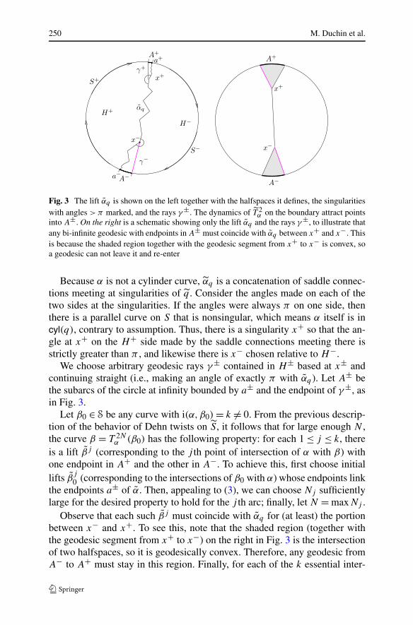
250 M. Duchin et al.
Fig. 3 The lift αq is shown on the left together with the halfspaces it defines, the singularitieswith angles > π marked, and the rays γ ±. The dynamics of T 2
α on the boundary attract pointsinto A±. On the right is a schematic showing only the lift αq and the rays γ ±, to illustrate thatany bi-infinite geodesic with endpoints in A± must coincide with αq between x+ and x−. Thisis because the shaded region together with the geodesic segment from x+ to x− is convex, soa geodesic can not leave it and re-enter
Because α is not a cylinder curve, αq is a concatenation of saddle connec-tions meeting at singularities of q . Consider the angles made on each of thetwo sides at the singularities. If the angles were always π on one side, thenthere is a parallel curve on S that is nonsingular, which means α itself is incyl(q), contrary to assumption. Thus, there is a singularity x+ so that the an-gle at x+ on the H+ side made by the saddle connections meeting there isstrictly greater than π , and likewise there is x− chosen relative to H−.
We choose arbitrary geodesic rays γ ± contained in H± based at x± andcontinuing straight (i.e., making an angle of exactly π with αq ). Let A± bethe subarcs of the circle at infinity bounded by a± and the endpoint of γ ±, asin Fig. 3.
Let β0 ∈ S be any curve with i(α,β0) = k �= 0. From the previous descrip-tion of the behavior of Dehn twists on S, it follows that for large enough N ,the curve β = T 2N
α (β0) has the following property: for each 1 ≤ j ≤ k, thereis a lift βj (corresponding to the j th point of intersection of α with β) withone endpoint in A+ and the other in A−. To achieve this, first choose initiallifts β
j
0 (corresponding to the intersections of β0 with α) whose endpoints linkthe endpoints a± of α. Then, appealing to (3), we can choose Nj sufficientlylarge for the desired property to hold for the j th arc; finally, let N = maxNj .
Observe that each such βj must coincide with αq for (at least) the portionbetween x− and x+. To see this, note that the shaded region (together withthe geodesic segment from x+ to x−) on the right in Fig. 3 is the intersectionof two halfspaces, so it is geodesically convex. Therefore, any geodesic fromA− to A+ must stay in this region. Finally, for each of the k essential inter-

Length spectra and degeneration of flat metrics 251
sections of β with α, we have shown that the curve β shares at least a saddleconnection with α. It follows that the geodesic representative of Tα(β) is nowexactly obtained from β by surgering in k copies of α, as in the discussionpreceding the Lemma. This completes the proof. �
Lemmas 19 and 20 imply Proposition 18. As an immediate corollary, itfollows that cyl(q) is determined by λS(q).
Corollary 21 If q, q ′ ∈ Flat(S) and λS(q) = λS(q′), then cyl(q) = cyl(q ′).
The next lemma shows that having the same set of cylinder curves is veryrestrictive.
Lemma 22 If cyl(q) = cyl(q ′), then Hq = Hq ′ .
Proof Suppose cyl(q) = cyl(q ′). First lift q and q ′ to arbitrary representativesin Q1, also called q and q ′, so that it is well-defined to talk about particular di-rections. Note that a cylinder curve, since it belongs a parallel family of non-singular representatives, has a well-defined direction θ ∈ RP1. Next, recallthat for any quadratic differential, the set of directions with at least one cylin-der is dense in RP1 by a result of Masur [21]. Thus, for every uniquely ergodicfoliation νθ
q ∈ P M F (q), there is a sequence of cylinder curves αi ∈ cyl(q) forwhich the directions converge: θi → θ . It follows that
νθiq → νθ
q as i → ∞.
Since i(νθiq , αi) = 0, it follows that in P M F , up to subsequence, we have
αi → μ ∈ P M F with i(μ, νθq ) = 0. Since νθ
q is uniquely ergodic, this meansthat μ and νθ
q are equal, and hence αi → νθq in P M F . From the assumption
that cyl(q ′) = cyl(q), it follows that νθq is also in P M F (q ′). Thus the sets of
uniquely ergodic foliations in P M F (q) and P M F (q ′) are identical.Consider a pair of uniquely ergodic foliations μ0 and ν0 in P M F (q) ∩
P M F (q ′). There is a matrix M (respectively, M ′) in SL2(R) so that μ0 andν0 are the vertical and the horizontal foliations of Mq (respectively, M ′q ′).However, there is a unique Teichmüller geodesic connecting μ0 and ν0 ([13]).Therefore, there is a time t for which
M ′q ′ = AtMq for At =(
et 00 e−t
).
That is, q ′ is in the SL(2,R) orbit of q , and hence Hq = Hq ′ . �
We can now assemble these facts together.

252 M. Duchin et al.
Proof of Theorem 1 Suppose λS(q) = λS(q′). By Corollary 21, cyl(q) =
cyl(q ′) and so Lemma 22 implies Hq = Hq ′ . A level set of the length of agiven cylinder curve on Hq = Hq ′ is a horocycle. So if α,β, γ ∈ cyl(q) =cyl(q ′) have distinct directions, then q and q ′ are contained in the intersectionof the same three distinct horocycles. As in the case of flat tori (Proposi-tion 17), this implies q = q ′. �
4 Iso-length-spectral families
Here we show constructively that for a set of curves to be spectrally rigid, itsprojectivization must not miss any open set of P M F .
Theorem 3 Suppose ξ(S) ≥ 2. If � ⊂ S ⊂ P M F and � �= P M F , thenthere is a deformation family � ⊂ Flat(S) for which � → R
� is constant,and such that the dimension of � grows linearly with ξ(S), as does thedimension of Flat(S) itself.
In particular, no finite set of curves determines a flat metric. We will builddeformation families of flat metrics in this section based on a train track argu-ment. We remind the reader of one specific fact which we will need (Propo-sition 23 below) and refer to [26] for a detailed discussion of train tracks.
A train track τ on S is said to be complete if all complementary regionsare either triangles or once-punctured monogons. By a weight on τ we meana nonnegative vector in R
B , where B is the set of branches of τ , satisfyingthe switch condition: the sum of the weights on all branches coming in to anyswitch is equal to the sum of the weights on the branches going out of thatswitch. We say that τ is recurrent if there is a weight on τ which is strictlypositive. An equivalent formulation of recurrence which is often easily veri-fied is that for each branch of τ there is a simple closed curve carried by τ
which traverses that branch (that is, the associated weight vector is positive onthat branch). The necessary result which we will need is the following conse-quence of [26, Theorem 2.7.4] regarding the set Uτ ⊂ P M L(S) of measuredlaminations carried by τ , which can be thought of as the projectivization ofthe space of weights on τ .
Proposition 23 If τ ⊂ S is a complete, recurrent train track, then Uτ containsan open subset of P M L(S).
Given a metric ρ on S (with metric completion S), we call a train track τ ⊂S magnetic with respect to ρ if there exists a magnetizing map f : (S,P ) →(S,P ), homotopic to the identity rel P , such that if γ ⊂ τ is a curve carriedby τ , then f (γ ) is a ρ-geodesic representative of γ (up to parametrization).

Length spectra and degeneration of flat metrics 253
The magnetizing map f should be thought of as taking a smooth realizationof the train track to a geodesic realization (compare Fig. 7 below). In theexamples in this section, f is a homeomorphism isotopic to the identity. Morecomplicated maps f are used to deal with the case of punctures, as presentedin the appendix.
Informally, a train track is magnetic if geodesics “stick to it”: geodesicscarried by τ actually live inside of the one-complex f (τ) as concatenationsof the branches. We will construct magnetic train tracks for flat metrics below,but remark that they do not exist for any hyperbolic metric (or in fact for anycomplete Riemannian metric), except when the train track is a simple closedcurve. We also note in passing that a complete magnetic train track can befound on any flat metric q ∈ Flat(S) by taking the geodesic representativeof any ending lamination with triangular complementary regions that is notstraight on q (i.e., not in P M L(q)). However, not every magnetic train trackadmits appropriate deformations, so we will take more care in this section toconstruct a deformable magnetic train track.
The strategy for proving Theorem 3 is to first construct an initial train trackτ on S and a deformation family ⊂ Flat(S) so that τ is magnetic in q for allq ∈ and so that the length of any curve γ carried by τ is constant on . Thetrain track τ we construct is complete and recurrent, and so by Proposition 23,Uτ ⊂ P M L has nonempty interior. Then, if � ⊂ S is not dense, we willfind a mapping class ψ adapted to � such that � ∈ ψUτ = Uψτ , and thedeformation family promised in the theorem will then be ψ.
The main ingredient needed to prove Theorem 3 is thus the following.
Proposition 24 If ξ(S) ≥ 2, then there exists a complete recurrent train trackτ and a positive-dimensional family of flat structures ⊂ Flat(S) such that:
• τ is magnetic in q for all q ∈ , and• the length of any curve γ carried by τ is constant on .
Proof If τ is a magnetic train track for a metric ρ, then there is a nonnegativelength assigned to each branch of τ (the length of its image under f ). Werecord this as a vector in R
B , where B is the set of branches of τ , and call itthe associated length vector for ρ. Then, the ρ-length of any curve carried byτ can be computed as the dot product of the weight vector for the curve withthe length vector for ρ.
To prove the proposition, we must construct the family ⊂ Flat(S) sothat the difference between the length vectors for any two q, q ′ ∈ lies inthe orthogonal complement of the space of weights on τ . Geometrically, thismeans that the difference in length vectors for q, q ′ ∈ can be distributedamong the switches so that at each switch, the increase in length of the in-coming branches is exactly equal to the decrease in length for each outgoingbranches; see Fig. 4.

254 M. Duchin et al.
Fig. 4 Changing the lengthvectors will be accomplishedby “folding or unfolding” atswitches which leaves thelength of curves carried bythe train track constant
Fig. 5 One basic buildingblock � and its train track τ .The cylinder C1 is picturedon the top and C2 on thebottom. Copies of � can beglued together end to end toobtain a copy of S
Fig. 6 Metric pictures of thetwo cylinders C1 (left) andC2 (right) which make up �
The idea is to build metrics and partial train tracks on “basic buildingblocks”, then glue them together in an appropriate pattern to obtain S. Forsimplicity, we only provide the details for closed surfaces in this section,as these can all simultaneously be handled by constructing a single build-ing block. To prove the theorem for all surfaces S with ξ(S) ≥ 2 it suffices toconstruct six more building blocks, using the same general ideas. For com-pleteness, we have included a description of these remaining building blocksin an appendix at the end of the paper.
The basic building block � is a genus-one surface with two boundary com-ponents described here and shown in Fig. 5. We will put a metric and a traintrack on �, and then assemble S from g −1 copies of � by gluing the bound-ary components in pairs. Choose nonperipheral arcs α (with endpoints a1, a2)and β (endpoints b1, b2) joining each boundary component to itself. Then thecomplement of those arcs is a pair of annuli. For any choice of t > 0, thereis a unique flat metric on � so that �(α) = �(β) = t , the two complementaryannuli Ci are Euclidean cylinders with boundary lengths 2t and heights t , anda1 is the closest point on its boundary circle to b1 on the other (the last re-quirement controls the twist—see Fig. 6). This means each cylinder will havearea 2t2, so � will have area 4t2.

Length spectra and degeneration of flat metrics 255
Choose the value of t so that 4t2(g −1) = 1 (in order that the glued surfacewill have total area one). After gluing g − 1 copies of � together end to end,we obtain a flat metric q0 on S, whose singular points come from the ai
and bi in the pieces �. We will choose to initially glue with a quarter-twist(compare Fig. 9), so that there are four evenly spaced singularities around thegluing curves, and these singularities all have cone angle 3π .
Next we build a one-complex T0 of geodesic segments in q0. In each piece�, let α′, α′′ be the minimal-length segments connecting a2 to b1 in C1, andlikewise β ′, β ′′ connecting a1 to b2 in C2 (the length of each of these willbe
√2t); see Fig. 5. Then the edges (branches) of T0 are the saddle con-
nections which belong to the boundary of a piece �, together with the arcsα,α′, α′′, β,β ′, β ′′ in those pieces. There are vertices (switches) for T0 at allof the singularities in the flat metric q0.
Each 1-cell of this complex T0 is smoothly embedded in S. However, thereis no well-defined tangent space at the switches. To obtain a train track τ ,we apply an appropriate homeomorphism F which is isotopic to the identity.For this, it suffices to specify at each switch which branches are incoming andwhich are outgoing. For each complex T occurring in the deformation family,every switch in T will have total angle 3π and five incident branches, one ofwhich is separated from its neighboring branches by angle π on each side.We use this to determine the tangencies as in Fig. 7.
Any curve γ ⊂ τ is mapped by f = F−1 to a concatenation of geodesicsegments which are branches of T0 = f (τ). But then any f (γ ) meets the an-gle conditions that suffice for geodesity (Remark 8), so τ is magnetic withrespect to q0. The complementary regions of the train track τ are triangles, soτ is complete. (We remark that this is a statement about the train track τ , andnot the graph T0, whose complementary 2-cells are not all triangles.) Further-more, it is straightforward to find sufficiently many curves carried by τ , thusshowing that it is recurrent.
Next we describe a deformation space 0 of q0 parameterized by 2(g − 1)
real numbers (small compared to t) so that a choice of parameters specifies a
Fig. 7 The homeomorphisms of S pictured here map between a geodesic one-complex T anda train track τ . This figure shows how to use the angles in T to read off the illegal turns ateach switch, which specifies the tangent spaces for τ . The inverse map f is the magnetizinghomeomorphism for τ with respect to the flat metric

256 M. Duchin et al.
modified flat metric q and geodesic 1-complex T . The 1-complex T is combi-natorially equivalent to T0 and satisfies the same necessary angle inequalitiesto guarantee that τ is magnetic in q , but the lengths have changed as pre-scribed by the parameters. The difference in corresponding length vectors ofq and q0 for τ will lie in the orthogonal complement of the space of weightvectors for τ , and hence we will have �q(α) = �q0(α) for every curve α car-ried by τ , as required.
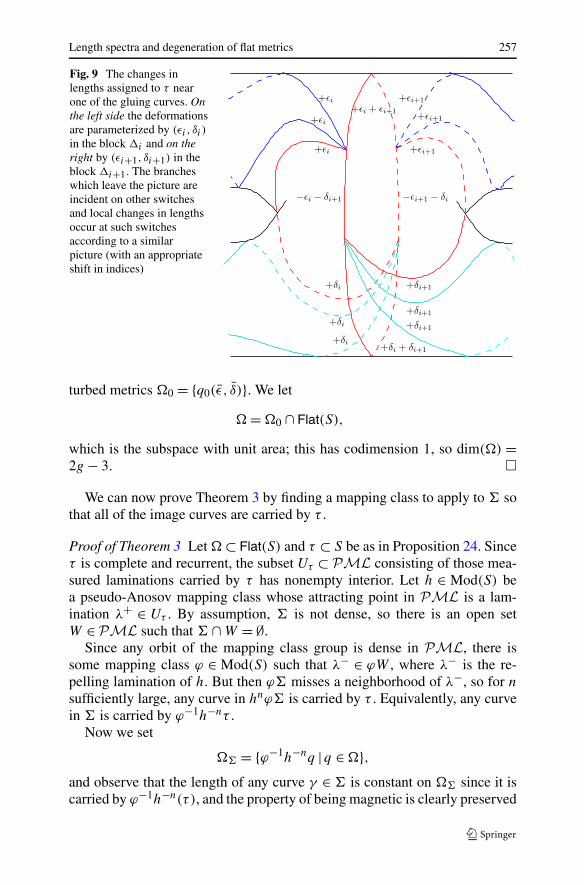
We carry out the deformations in each block, and then glue the pieces to-gether appropriately. In each block �, the deformations are parameterized bytwo numbers ε and δ (small compared to t) so that the change in lengths ofedges is given by the following table.
A1 A2 B1 B2 α α′ α′′ β β ′ β ′′+ε − δ −ε + δ +ε − δ −ε + δ +ε + δ +2ε +2ε +ε + δ +2δ +2δ
We now verify that (a) this change in lengths can be realized by a flat metricbuilt from Euclidean cylinders similar to the construction above, and (b) aftergluing all the pieces, the change in length vectors is orthogonal to the spaceof weight vectors.
To verify (a), we refer to Fig. 8 which shows how the required changes inlength data are metrically realized by deformations of the Euclidean cylin-ders.
For (b), let εi, δi denote the parameters of the deformation of the ith block�i . To guarantee that the difference in length vectors is orthogonal to thespace of weight vectors, we must be able to distribute the difference vectoramong the switches so that the increase in length of the incoming branches isexactly equal to the decrease in length for each outgoing branches. One cancheck that the change in lengths near the switches shown in Fig. 9 satisfiesthis condition, and moreover the deformations on each �i (as described bythe table) can be glued to accomplish this change.
If we write (ε, δ) = (ε1, δ1, . . . , εg−1, δg−1) for the vector of the parame-ters, then we obtain a 2(g − 1)-dimensional deformation space from the per-
Fig. 8 We have two parameters ε, δ to perturb the flat structures in each piece �. Metrically,this can be achieved by deforming the rectangles to parallelograms, adjusting the height andshear appropriately. (Compare Fig. 6)
Length spectra and degeneration of flat metrics 257
Fig. 9 The changes inlengths assigned to τ nearone of the gluing curves. Onthe left side the deformationsare parameterized by (εi , δi )
in the block �i and on theright by (εi+1, δi+1) in theblock �i+1. The brancheswhich leave the picture areincident on other switchesand local changes in lengthsoccur at such switchesaccording to a similarpicture (with an appropriateshift in indices)
turbed metrics 0 = {q0(ε, δ)}. We let
= 0 ∩ Flat(S),
which is the subspace with unit area; this has codimension 1, so dim() =2g − 3. �
We can now prove Theorem 3 by finding a mapping class to apply to � sothat all of the image curves are carried by τ .
Proof of Theorem 3 Let ⊂ Flat(S) and τ ⊂ S be as in Proposition 24. Sinceτ is complete and recurrent, the subset Uτ ⊂ P M L consisting of those mea-sured laminations carried by τ has nonempty interior. Let h ∈ Mod(S) bea pseudo-Anosov mapping class whose attracting point in P M L is a lam-ination λ+ ∈ Uτ . By assumption, � is not dense, so there is an open setW ∈ P M L such that � ∩ W = ∅.
Since any orbit of the mapping class group is dense in P M L, there issome mapping class ϕ ∈ Mod(S) such that λ− ∈ ϕW , where λ− is the re-pelling lamination of h. But then ϕ� misses a neighborhood of λ−, so for n
sufficiently large, any curve in hnϕ� is carried by τ . Equivalently, any curvein � is carried by ϕ−1h−nτ .
Now we set
� = {ϕ−1h−nq |q ∈ },and observe that the length of any curve γ ∈ � is constant on � since it iscarried by ϕ−1h−n(τ ), and the property of being magnetic is clearly preserved
258 M. Duchin et al.
when both the train track and the metric are modified by the same mappingclass. �
Remark 25 Here, we obtain a deformation family of dimension 2g − 3. Wemake no claim that this is optimal, but note that the optimal dimension isbounded above and below by linear functions in g, since Flat(S) itself hasdimension 12g − 14. For the cases covered in the appendix, which allowpunctures and boundary components, this proportionality holds as well: thenumber of parameters in the deformation space is linearly comparable to g +n, as is the complexity of S and therefore the dimension of Flat(S).
5 Flat structures as currents
Bonahon’s space of geodesic currents derives its utility from the fact that somany spaces embed into it in natural ways with respect to the intersectionform. For example, the space of measured laminations M L, being the com-pletion of S with respect to i, is easily seen to embed into C(S), and the re-striction of i to M L × M L is Thurston’s continuous extension of geometricintersection number from weighted simple curves to measured laminations.In this section, we see that Flat(S) embeds naturally as well.
For closed surfaces, Bonahon constructs an embedding of T (S) into C(S)
in [4] by sending a hyperbolic metric m to its associated Liouville currentLm. This was extended to all negatively curved Riemannian metrics by Otalin [24] and to negatively curved cone metrics by Hersonsky–Paulin in [16].Given any such metric m, we will denote the associated current by Lm. Thenaturality with respect to i is expressed by the equation
i(Lm,α) = �m(α).
This extends easily to Flat(S), and in fact it is possible to carry out thisconstruction for surfaces which are not necessarily closed. Given q ∈ Q1(S),we can view θ �→ νθ
q as a map RP1 → C(S).
Proposition 26 For any q ∈ Flat(S) there exists a current Lq such that
(1) for all α ∈ C′, i(Lq,α) = �q(α);
(2) for all μ ∈ C(S) and any q ∈ Q1(S) inducing the given q ∈ Flat(S),
i(Lq,μ) = 1
2
∫ π
0i(νθ
q ,μ)dθ;
(3) i(Lq,Lq) = π/2.

Length spectra and degeneration of flat metrics 259
Proof We can define Lq by a Riemann integral
Lq = 1
2
∫ π
0νθq dθ
by which we mean a limit of Riemann sums. Since RP1 is compact, the mapf (θ) = νθ
q is uniformly continuous. As the metric d from Theorems 12 and 16is complete, this integral exists.
For any α ∈ C′, we recall the formula from Lemma 9
�q(α) = 1
2
∫ π
0i(νθ
q , α) dθ.
Combining this with the uniform continuity of νθq implies part (1) and also
part (2) for any current μ which is a scalar multiple of a current associated toa curve. For general currents we appeal to the density of R+ × C in C(S) andthe continuity of intersection number.
The foliations νθq have q-length 1, and so i(Lq, νθ
q ) = 1 (this also followsfrom part (2)). Therefore, (3) follows from (2) by the computation
i(Lq,Lq) = 1
2
∫ π
0i(Lq, ν
θq ) dθ = 1
2
∫ π
0dθ = π
2. �
Remark 27 In the closed case, an equivalent definition of Lq can be given asa cross-ratio, as in Hersonsky-Paulin.
This proposition provides the tools needed to give the embedding ofFlat(S) into C(S).
Theorem 4 There is an embedding
Flat(S) → C(S)
denoted by q �→ Lq so that for q ∈ Flat(S) and α ∈ C′, we have i(Lq,α) =�q(α). Furthermore, after projectivizing, Flat(S) → P C(S) is still an embed-ding.
Proof If qn → q in Flat(S), then �qn(α) → �q(α) for all α ∈ C′, and henceLqn → Lq by Theorems 12 and 16. Thus, q �→ Lq is continuous.
Injectivity for Flat(S) → C(S) follows directly from Theorem 1, wherewe have shown that even intersection with elements of S distinguishes flatmetrics. Injectivity for Flat(S) → P C(S) follows from the fact that i(Lq,Lq)
is constant, which ensures that no two currents in the image of Flat(S) can bemultiples of one another.
Therefore, Flat(S) continuously injects into C(S). To show that this map isan embedding, we need to show that if qn exits every compact set in Flat(S),

260 M. Duchin et al.
then Lqn has no subsequence which converges to a point of (the image of)Flat(S). This is a consequence of Theorem 5 proven below, which describesprecisely the subsequential limits of Lqn . �
As a consequence of the continuity of Flat(S) → C(S), we find that thelength of a lamination in a flat metric is well-defined, and moreover theselengths vary continuously.
Corollary 28 The flat-length function Flat(S) × S(S) → R has a continuoushomogeneous extension
� : Flat(S) × M F (S) → R
given by
(q,μ) �→ �q(μ) = i(Lq,μ).
We can now prove the main theorem.
Theorem 2 If ξ(S) ≥ 2, then � ⊂ S ⊂ P M F is spectrally rigid over Flat(S)
if and only if � is dense in P M F .
Proof We first assume � is dense in P M F . Suppose q, q ′ ∈ Flat(S) have�q(α) = �q ′(α) for all α ∈ �. For any μ ∈ M F , the density hypothesis im-plies that there are scalars ti and curves αi ∈ � such that tiαi → μ. But
�q(tiαi) = �q ′(tiαi),
so Corollary 28 implies �q and �q ′ agree on μ. In particular, the two metricsassign the same length to all simple closed curves. By Theorem 1, it followsthat q = q ′, and thus � is spectrally rigid.
Next assume that � is not dense in P M F . Theorem 3 implies the exis-tence of a positive-dimensional family � ⊂ Flat(S) for which the lengths ofcurves in � is constant. In particular, there exists a pair of distinct flat struc-tures q, q ′ ∈ � for which �q(α) = �q ′(α) for all α ∈ �, and hence � is notspectrally rigid. �
6 The boundary of Flat(S)
In this section we give a description of the geodesic currents that appear inthe closure of Flat(S) ⊂ P C(S). We will show that the limit points have geo-metric interpretations as a hybrid of a flat structure on some subsurface and ageodesic lamination on a disjoint subsurface (Theorem 5). We call such cur-rents mixed structures. As a first step, we show that the description of Lq as

Length spectra and degeneration of flat metrics 261
average intersection number with foliations νθq (Proposition 26, part (2)) ex-
tends to any limiting geodesic current. This description greatly simplifies theanalysis of what geodesic currents can appear as degenerations of flat metrics.
To every nonzero quadratic differential, we consider again the map
RP1 → M L(q) ⊂ M L(S)
given by θ �→ νθq , the foliation in direction θ . We show that given a sequence
of quadratic differentials whose associated currents converge in C(S), thesemaps converge uniformly (up to subsequence) to a continuous map from RP1
to M L(S).
Lemma 29 For all q ∈ Q1(S), α ∈ C′, and angles θ0 and θ1, we have
∣∣ i(νθ1q , α) − i(νθ0
q , α)∣∣ ≤ �q(α) · |θ1 − θ0|.
It follows that θ �→ νθq is Lipschitz.
Proof Let ω be a saddle connection contained in a q-geodesic representativeof α. Assume ω is at angle φ. We have i(νθ
q ,ω) = �q(ω) · | sin(θ −φ)|. Hence
∣∣∣∣ d
dθi(νθ
q ,ω)
∣∣∣∣ = �q(ω) · | cos(θ − φ)| ≤ �q(ω).
Integrating the above inequality from θ0 to θ1 and adding up over all saddleconnections of α proves the lemma. �
Proposition 30 Let qn be a sequence of quadratic differentials so that snLqn
converges in C(S) to a geodesic current L∞. Then, after possibly passing toa subsequence, the sequence of functions
fn : RP1 → M L(S), fn(θ) = snνθqn
converges uniformly to a continuous function
f∞ : RP1 → M L(S).
Proof We can consider fn as maps from RP1 to C(S). Since M L(S) is aclosed subset of C(S), the image of the limiting map f∞ is automatically inM L(S), provided it exists.
Equip C(S) with the metric in Theorem 12 (or 16 for punctured surfaces).By the Arzelá-Ascoli theorem, it is sufficient to show that the family of mapsfn is equicontinuous and the union of the images have compact closure. For

262 M. Duchin et al.
angles θ0 and θ1 we have
d(fn(θ1), fn(θ0)
) =∑
α∈C′(S)
sntα∣∣ i(νθ1
qn, α) − i(νθ0
qn, α)
∣∣
≤ |θ1 − θ0|∑
α∈C′(S)
sntα �qn(α)
= |θ1 − θ0| · d(snLqn,0).
The inequality follows from Lemma 29, and the equalities are immediatefrom the definition of the metric, together with Proposition 26. Since
d(snLqn,0) → d(L∞,0),
there exists K > 0 such that d(snLqn,0) ≤ K , and so the family of maps {fn}is equicontinuous.
It remains to show that the⋃
n fn(RP1) has compact closure. Observe that
i(fn(θ), α) = i(snνθq , α) ≤ sn�qn(α).
Therefore,
d(fn(θ),0) =∑
α∈C′(S)
tα i(fn(θ), α) ≤∑
α∈C′(S)
sntα�qn(α) = d(snLqn,0).
and so⋃
n fn(RP1) is contained in the closed K-ball about 0. Since d is
proper, this ball is compact. �
We now define mixed structures on S. This requires us to first make precisewhat we will mean by a flat structure on a subsurface.
Suppose X ⊂ S is a π1-injective subsurface of S with negative Euler char-acteristic. We view X as a punctured surface (removing every boundary com-ponent), and let Flat(X) denote the space of flat structures on X. By thiswe mean a flat structure on each component of X as described in Sect. 2.3,where we now require the sum of the areas of the components to be one.The boundary curves of X are realized by punctures and hence have length 0.Equivalently, an element of Flat(X) is given by a unit-norm quadratic dif-ferential in Q(X), nonzero on all components, and well-defined up to mul-tiplication by a unit-norm complex number in each component. Represent-ing any q ∈ Flat(X) by a unit-norm quadratic differential, we have the mapRP1 → M L(X) given by θ �→ νθ
q as before. Extending measured laminationson X to measured laminations on S in the usual way, we can view θ �→ νθ
q asa map into M L(S) ⊂ C(S).

Length spectra and degeneration of flat metrics 263
Given a subsurface X ⊂ S as above, q ∈ Flat(X), and a measured lamina-tion λ ∈ M L(S) whose support can be homotoped disjoint from X, we definea mixed structure η = (X,q,λ) to be the geodesic current given by
η = λ + 1
2
∫ π
0νθq dθ.
Here the integral is a Riemann integral, as in the proof of Proposition 26. Forbrevity we can write η = λ + Lq . It follows that for every α ∈ C′(S),
i(η,α) = i(λ,α) + 1
2
∫ π
0i(νθ
q , α) dθ.
We also allow the two degenerate situations X = S and X = ∅. In these cases,the corresponding mixed structure is a flat structure on S or a measured lam-ination on S, respectively.
Now let Mix(S) ⊂ C(S) denote the space of all mixed structures, andP Mix(S) its image in P C(S) under the projection C(S) → P C(S). Observethat if
η ∈ Mix(S) \ M L(S)
then i(η, η) = π/2, just as in Proposition 26.If α is a curve in ∂X, then i(νθ
q , α) = 0 and i(λ,α) = 0. Hence i(η,α) = 0,although α may be contained in the support of λ (and thus η).
Theorem 5 The closure of Flat(S) in P C(S) is exactly the space P Mix(S) ofprojective mixed structures. That is, for any sequence {qn} in Flat(S), afterpassing to a subsequence if necessary, there exists a mixed structure η and asequence of positive real numbers {tn} so that
limn→∞ tn�qn(α) = i(α, η)
for every α ∈ C. Moreover, every mixed structure is the limit of a sequence inFlat(S).
Proof Let qn be a sequence of quadratic differentials such that tnLqn → L∞,for some sequence of positive real numbers tn. We have to show that, up toscaling, L∞ ∈ Mix(S).
If the sequence tn converges to zero, then
i(L∞,L∞) = limn→∞ t2
n i(Lqn,Lqn) = π
2lim
n→∞ t2n = 0.
That is, L∞ is a measured lamination (c.f. Bonahon [4]). Thus the theoremholds with X = ∅.

264 M. Duchin et al.
Since every geodesic current has finite self-intersection number, we canconclude that tn does not tend to infinity. Therefore, after taking a subse-quence, we can assume that the sequence tn is convergent, and in fact con-verges to 1. That is, there is a geodesic current (which we again denote byL∞) such that Lqn → L∞ in C(S). Applying Proposition 30 and taking afurther subsequence if necessary, we can also assume that fn converges uni-formly to a continuous map f∞. As a consequence, for every curve α ∈ C,
i(L∞, α) = 1
2
∫ π
0i(f∞(θ), α
)dθ.
Define S0 ⊂ S to be the set of simple closed curves α for which�qn(α) → 0. Equivalently, α ∈ S0 if and only if i(L∞, α) = 0. Let Z0 bethe subsurface of S that is filled by S0. That is, up to isotopy, Z0 is the largestπ1-injective subsurface Z (with respect to containment) having the propertythat every closed curve in S which cuts Z has positive intersection numberwith some curve in S0. If Z0 = S, then there is a finite set α1, . . . , αk ofcurves in S0 such that
∑αi is a binding current, and as L∞ lies in the span
of M L(S) ⊂ C(S), we have∑
i(L∞, αi) > 0,
which is a contradiction. Therefore, Z0 is a proper subsurface of S.We observe that, for each α0 ∈ S0,
1
2
∫ π
0i(α0, f∞(θ)) dθ = i(L∞, α0) = 0.
Since f∞ is continuous, this implies that i(α0, f∞(θ)) = 0 for every θ . Thatis, for every θ ∈ RP1, the support of f∞(θ) can be homotoped to be disjointfrom Z0. Hence, i(α,L∞) = 0 for every essential curve in Z0. However, therestriction of L∞ to Z0 may not be zero; for an annular component A of Z0,the restriction of f∞(θ) to A may be a measured lamination that is supportedon the core curve of A.
Now choose a component W of S \ Z0. Define
D(W) ={
i
(L∞,
α
�q0(α)
)∣∣∣∣α ∈ S(W)
}.
Observe that D(W) is bounded, since { α�q0 (α)
} is precompact, being contained
in the compact set
{λ ∈ M L(S) |�q0(λ) = 1}.We argue in two cases.

Length spectra and degeneration of flat metrics 265
Case 1: inf(D(W)) > 0.In this case, we have a uniform lower bound for the qn-length of any nonpe-
ripheral simple closed curve, and hence also any nonperipheral closed curvein W . Since W is a component of S \ Z0, the qn-lengths of the boundarycurves of W go to zero. Therefore, after choosing a basepoint in W (awayfrom the boundary) and passing to a subsequence, we can assume that qn|Wconverges to a flat structure on W geometrically, that is, after re-markingby a homeomorphism. (See Appendix A of [22] for a thorough discussionof the geometric topology on the space of quadratic differentials. In particu-lar, McMullen establishes the existence of the relevant geometric limit in hisTheorem A.3.1 for points in moduli space.) Since any given curve in W hasa uniform upper bound to its qn-length, we may assume that the re-markinghomeomorphisms are isotopic to the identity in W , and hence qn|W convergesto a flat structure on W (though not necessarily of unit area).
Case 2: inf(D(W)) = 0.In this case, we have a sequence of simple curves αn ∈ C(W) such that
limn→∞ i
(L∞,
αn
�q0(αn)
)= 0.
Since { αn
�q0 (αn)} is precompact, we may pass to a subsequence so that
αn
�q0(αn)→ λ,
for some lamination λ. The continuity of intersection number impliesi(L∞, λ) = 0.
We observe that λ has to fill W . To see this, let W ′ ⊂ W be the subsurfacefilled by λ. Since i(L∞, λ) = 0, it follows that i(f∞(θ), λ) = 0. Therefore,i(f∞(θ), ∂W ′) = 0 and hence i(L∞, ∂W ′) = 0. Thus ∂W ′ ∈ S0 and W = W ′.The support of L∞ consists of geodesics having no transverse intersectionwith the support of λ. Therefore, the support of L∞, restricted to W , equalsthe support of λ. That is, L∞|W is a (filling) measured lamination in W .
We have shown that L∞ is a mixed structure (X,q,λ) where X is the unionof all W as in Case 1, q is the limiting flat structure in X and λ is the unionof limiting laminations in Case 2 and weighted curves from all the annularcomponents A where the restriction of some f∞(θ) to A is nontrivial. Since
i(L∞,L∞) = limn→∞ i(Lqn,Lqn) = π/2,
the sum of the areas of the flat structures is 1.To finish the proof, we show that any mixed structure η = (X,q,λ) appears
as the limit of a sequence of flat structures. The idea is to build the metric

266 M. Duchin et al.
from q on X, by making small slits at the punctures and gluing in a sequenceof metrics on the complement, limiting to λ and with area tending to zero.
First lift q to an arbitrary representative q ∈ Q1(X). Next write the lami-nation λ as λ = λ0 + λ1, where λ0 is supported on a disjoint union of simpleclosed curves, and λ1 has support a lamination with no closed leaves. We canfurther decompose λ0 = ∑
i siαi for some αi ∈ S and si > 0. For each i andall n ≥ 0, let Ci,n be a Euclidean cylinder with height si and circumference2/n2. Let Y be the subsurface filled by λ1 (with boundary replaced by punc-tures) and let q ′ ∈ Q1(Y ) be any quadratic differential for which ν0
q ′ = λ1.Consider the Teichmüller deformation Anq
′, where
An =(
n 00 1
n
).
This tends to the vertical foliation of q ′ (which was chosen to be λ1) by Propo-sition 33 below.
Let Z be the union of the nonannular, non-pants components of S \(X∪Y).Choose any quadratic differential q ′′ ∈ Q1(Z) for which the vertical foliationis minimal (for simplicity).
Now we construct a flat structure qn as follows. At each puncture in q thatcorresponds to an essential curve in S (that is, a boundary component of X inS) we cut open a slit of size 1/n2 emanating from the given puncture, in anydirection. Similarly, letting
q ′(n) = 1
nAnq
′ and q ′′(n) = 1
nq ′′,
cut open slits of length 1/n2 along the vertical foliations of each, one startingat each of the punctures of Y and Z that correspond to essential curves in S.Note that since the vertical foliations of q ′(n) and q ′′(n) are minimal, theseconstructions are possible. We glue these and the cylinders {Ci,n} along theirboundaries to recover the surface S with a quadratic differential qn, which wescale to have unit norm (as n tends to infinity, the areas of q ′(n) and q ′′(n)
go to zero and the scaling factor tends to 1). We glue along the boundariesby a local isometry, and if we further require the relative twisting of q0 andqn along every gluing curve to be uniformly bounded, we obtain a sequencelimiting to η in P C(S), as desired. �
A dimension count The Thurston boundary is very nice as a topologicalspace: it is a sphere compactifying a ball, having codimension one in thecompactification T (S). Here, we show that the codimension of ∂Flat(S) isthree. To see this, first recall that for a connected surface S of genus g with n
punctures, T (S) is (6g + 2n − 6)-dimensional. The space Q(S) of quadratic
Length spectra and degeneration of flat metrics 267
differentials on S has twice the dimension and Flat(S) is a quotient of Q(S)
by an action of C. Hence
dim(Flat(S)) = 12g + 4n − 14.
For any π1-injective subsurface Y ⊂ S, we consider the subset ∂Y ⊂∂Flat(S) consisting of those η = (X,q,λ) for which the support of the flatmetric is X = S \ Y . Observe that ∂Flat(S) is a disjoint union of subsets ofthe form ∂Y , as Y varies over subsurfaces of S. In the case that Y is an annuluswith core curve α, we simply write ∂Y = ∂α . Points in ∂α are projective mixedstructures of the form wα + Lq , where q ∈ Flat(X) and the weights w on α
are nonnegative numbers. We first compute the dimension of the sets ∂α .If α is a non-separating curve, then X is connected, has genus one less than
S and has 2 extra punctures. That is,
dim(Flat(X)) = 12(g − 1) + 4(n + 2) − 14 = 12g + 4n − 18.
To recover the space ∂α , we restore one extra dimension from the weight onα, so that dim(∂α) = 12g +4n−17, giving that space codimension three withrespect to Flat(S).
Now let α be a separating curve. Then X = X1 ∪X2, where Xi is a surfaceof genus gi with ni punctures (i = 1,2) so that g = g1 + g2 and n = n1 +n2 − 2. Therefore, Q(X) has dimension
(12g1 + 4n1 − 12) + (12g2 + 4n2 − 12) = 12g + 4(n + 2) − 24
= 12g + 4n − 16.
The space Flat(X) is the quotient of Q(X) by scaling and rotation in eachcomponent, but the total area must be one in the end, giving
dim(Flat(X)) = dim(Q(X)) − 3 = 12g + 4n − 19.
The space ∂α has one extra dimension from the weight on α and is (12g +4n − 18)-dimensional. In the separating case, then, the codimension is fourwith respect to Flat(S).
It is not difficult to see that for larger-complexity subsurfaces Y ⊂ S, thesubsets ∂Y have higher codimension in Flat(S), since for any subsurface W ,
dim M L(W) < dim Flat(W).
Since ∂Flat(S) is a countable union of sets of the form ∂Y , each of which canbe exhausted by compact (hence closed) sets, the dimension of ∂Flat(S) is themaximum dimension of any subset ∂Y (by the Sum Theorem in [23]), whichis therefore 12g + 4n − 16. So we have seen that ∂Flat(S) has codimensionthree in Flat(S).

268 M. Duchin et al.
7 Remarks and questions
7.1 Rigidity for closed curves
Though we have a complete description of rigidity for � ⊂ S, the more gen-eral case of � ⊂ C is still open.
We have already seen a sufficient condition for � ⊂ C to be spectrallyrigid over flat metrics: clearly if P M F ⊂ P(�), then � is spectrally rigidbecause its lengths determine all those from S in that case. Here is a furtherobservation.
Proposition 31 If S is closed and � has nonempty interior as a subset ofC(S), then � is spectrally rigid over any class of metrics that embeds natu-rally into C(S).
Proof Fix a pair of currents ν1,ν2 and set
f (μ) := i(ν1,μ) − i(ν2,μ).
Suppose there is an open set in f −1(0), which we can assume is Bε(μ0), theε-ball about some point μ0 in the metric from Theorem 12. By the linearityof i and the definition of the metric, μ0 + δ ∈ Bε(μ0) for any δ ∈ Bε(0), andsince f (μ0 + δ) = 0, we have f (δ) = 0. But every current is a multiple of acurrent in Bε(0) and f is linear, so this shows that ν1 and ν2 have the sameintersection number with all of the elements of C(S). We can conclude thatν1 = ν2 by Otal’s theorem. In fact, we have shown that intersections with anyopen set of currents suffice to separate points in C(S).
To apply this to a class of metrics such that G(S) ↪→ C(S) and i(Lρ,α) =�ρ(α), suppose that λ�(ρ) = λ�(ρ′). Letting
ν1 = Lρ and ν2 = Lρ′,
we have f (μ) = 0 for all μ ∈ �, which contains an open set by assumption.This then implies that ρ = ρ′. �
7.2 Remarks on the boundary of Flat(S)
Remark 32 (Visibility in the boundary) We observe that Teichmüller geodes-ics behave well with respect to the compactification of Flat(S). For all thepoints along a Teichmüller geodesic, the vertical and horizontal foliations areconstant, up to scaling. In this compactification, every geodesic limits to itsvertical foliation.

Length spectra and degeneration of flat metrics 269
Proposition 33 Let G : R → T (S) be a Teichmüller geodesic, let qt be thecorresponding quadratic differential at time t and ν0 be the initial verticalfoliation at q0. Then, considering ν0 as an element of C(S), we have
Lqt
et→ ν0.
Proof The flat length of a curve is less than the sum of its horizontal lengthand its vertical length and is larger than the minimum of its horizontal andvertical lengths. That is, if μt and νt are the horizontal and the vertical folia-tion at qt then for every α ∈ C′(S) we have
min(
i(α, νt ), i(α,μt)) ≤ �qt (α) ≤ i(α, νt ) + i(α,μt).
But i(α, νt ) = et i(α, ν0) and i(α,μt) = e−t i(α,μ0). Therefore,
i(Lqt , α)
et= �qt (α)
et→ i(α, ν0).
Theorems 11 and 15 assure us that a current is completely determined bythese intersections. �
This proposition shows not only that points along a Teichmüller geodesicconverge to a unique limit in ∂Flat(S) = P Mix(S), but also that different geo-desic rays with a common basepoint have different limit points in the bound-ary (because they have different vertical foliations). This is in contrast withthe situation for the Thurston boundary where both of the above statementsare false (see [18] and [20]).
Remark 34 (Compatibility with the Thurston boundary) The boundary ofFlat(S) described here and the Thurston boundary of Teichmüller space arecompatible in a certain sense. Consider the projection
σ : Flat(S) → T (S)
which sends a flat metric q to the hyperbolic metric in its conformal class.As flat structures degenerate to the boundary, the corresponding hyperbolicmetrics accumulate in P M L. The following proposition describes the rela-tionship between the limiting structures: they have zero intersection number.The results on Teichmüller geodesics in the previous remark illustrate a spe-cial case of this.
Proposition 35 Let qn be a sequence of flat structures on S and σn = σ(qn).Assume that σn → μ in the Thurston compactification and qn → η in P C(S),where μ is a geodesic lamination and η is a mixed structure in ∂Flat(S). Then
i(μ,η) = 0.
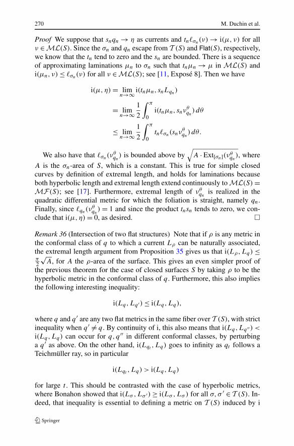
270 M. Duchin et al.
Proof We suppose that snqn → η as currents and tn�σn(ν) → i(μ, ν) for allν ∈ M L(S). Since the σn and qn escape from T (S) and Flat(S), respectively,we know that the tn tend to zero and the sn are bounded. There is a sequenceof approximating laminations μn to σn such that tnμn → μ in M L(S) andi(μn, ν) ≤ �σn(ν) for all ν ∈ M L(S); see [11, Exposé 8]. Then we have
i(μ,η) = limn→∞ i(tnμn, snLqn)
= limn→∞
1
2
∫ π
0i(tnμn, snν
θqn
) dθ
≤ limn→∞
1
2
∫ π
0tn�σn(snν
θqn
) dθ.
We also have that �σn(νθqn
) is bounded above by√
A · Ext[σn](νθqn
), where
A is the σn-area of S, which is a constant. This is true for simple closedcurves by definition of extremal length, and holds for laminations becauseboth hyperbolic length and extremal length extend continuously to M L(S) =M F (S); see [17]. Furthermore, extremal length of νθ
qnis realized in the
quadratic differential metric for which the foliation is straight, namely qn.Finally, since �qn(ν
θqn
) = 1 and since the product tnsn tends to zero, we con-clude that i(μ,η) = 0, as desired. �
Remark 36 (Intersection of two flat structures) Note that if ρ is any metric inthe conformal class of q to which a current Lρ can be naturally associated,the extremal length argument from Proposition 35 gives us that i(Lρ,Lq) ≤π2
√A, for A the ρ-area of the surface. This gives an even simpler proof of
the previous theorem for the case of closed surfaces S by taking ρ to be thehyperbolic metric in the conformal class of q . Furthermore, this also impliesthe following interesting inequality:
i(Lq,Lq ′) ≤ i(Lq,Lq),
where q and q ′ are any two flat metrics in the same fiber over T (S), with strictinequality when q ′ �= q . By continuity of i, this also means that i(Lq,Lq ′′) <
i(Lq,Lq) can occur for q, q ′′ in different conformal classes, by perturbinga q ′ as above. On the other hand, i(Lqt ,Lq) goes to infinity as qt follows aTeichmüller ray, so in particular
i(Lqt ,Lq) > i(Lq,Lq)
for large t . This should be contrasted with the case of hyperbolic metrics,where Bonahon showed that i(Lσ ,Lσ ′) ≥ i(Lσ ,Lσ ) for all σ,σ ′ ∈ T (S). In-deed, that inequality is essential to defining a metric on T (S) induced by i
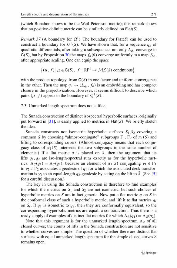
Length spectra and degeneration of flat metrics 271
(which Bonahon shows to be the Weil-Petersson metric); this remark showsthat no positive-definite metric can be similarly defined on Flat(S).
Remark 37 (A boundary for Q1) The boundary for Flat(S) can be used toconstruct a boundary for Q1(S). We have shown that, for a sequence qn ofquadratic differentials, after taking a subsequence, not only Lqn converge inC(S), but by Proposition 30 the maps fn(θ) converge uniformly to a map f∞,after appropriate scaling. One can equip the space
{(μ,f )
∣∣μ ∈ C(S), f : RP1 → M L(S) continuous}
with the product topology, from C(S) in one factor and uniform convergencein the other. Then the map qn �→ (Lqn, fn) is an embedding and has compactclosure in the projectivization. However, it seems difficult to describe whichpairs (μ,f ) appear in the boundary of Q1(S).
7.3 Unmarked length spectrum does not suffice
The Sunada construction of distinct isospectral hyperbolic surfaces, originallyput forward in [31], is easily applied to metrics in Flat(S). We briefly sketchthe idea.
Sunada constructs non-isometric hyperbolic surfaces S1,S2 covering acommon S by choosing “almost-conjugate” subgroups �1,�2 of π1(S) andlifting to corresponding covers. (Almost-conjugacy means that each conju-gacy class of π1(S) intersects the two subgroups in the same number ofelements.) If a flat metric q is placed on S, then the argument that itslifts q1, q2 are iso-length-spectral runs exactly as for the hyperbolic met-rics: �C(q1) = �C(q2), because an element of π1(S) conjugating γ1 ∈ �1to γ2 ∈ �2 associates a geodesic of q1 for which the associated deck transfor-mation is γ1 to an equal-length q2-geodesic by acting on the lift to S. (See [5]for a careful discussion.)
The key in using the Sunada construction is therefore to find examplesfor which the metrics on S1 and S2 are not isometric, but such choices ofhyperbolic metrics on S are in fact generic. Now put a flat metric q on S inthe conformal class of such a hyperbolic metric, and lift it to flat metrics qi
on Si . If q1 is isometric to q2, then they are conformally equivalent, so thecorresponding hyperbolic metrics are equal, a contradiction. Thus there is aready supply of examples of distinct flat metrics for which �C(q1) = �C(q2).
Note that this argument is for the unmarked length spectrum �C of allclosed curves; the counts of lifts in the Sunada construction are not sensitiveto whether curves are simple. The question of whether there are distinct flatsurfaces with equal unmarked length spectrum for the simple closed curves S
remains open.

272 M. Duchin et al.
Acknowledgements This work began while all three authors were visiting MSRI in Berke-ley, CA for the Fall 2007 programs on Teichmüller theory and Kleinian groups and Geometricgroup theory. We would like to thank MSRI and all of the participants for providing such astimulating mathematical environment. We thank Daryl Cooper for discussions of his work onprojective structures that suggested the idea of mixed structures. Finally, we thank the anony-mous referee for thorough and helpful comments.
Appendix: More building blocks
Here we sketch the construction of the remaining basic building blocksneeded to carry out the proof of Proposition 24 for a general surface S withξ(S) ≥ 2. The building blocks are surfaces �g,n,b where g is the genus, n,is the number of punctures/marked points, and b is the number of boundarycomponents. If we let d denote the dimension of the space of metrics weconstruct on �g,n,b, then the resulting pairs (�g,n,b, d) are:
(�1,0,2,2), (�1,0,1,2), (�1,1,1,2), (�0,2,1,0), (�0,3,1,2), (�0,4,1,2),
(�0,4,2,3).
The case of �1,0,2 was discussed in Sect. 4. Each building block will comeequipped with a train track that carries the boundary, and when the buildingblocks are assembled to construct the surface S, the train tracks assemble toa complete recurrent train track. The family of metrics for each will keep theboundary length fixed, so that the deformations can be carried out indepen-dently on each piece. Gluing together the deformations is carried out in afashion similar to that used for the closed case in Sect. 4.
By gluing the pieces above, one can construct flat structures and magnetictrain-tracks on any surface with ξ ≥ 2. In sketch, one can attach along theirboundaries copies of �1,0,2 (to add one to the genus) and �0,4,2 (to add fourpunctures) to obtain a surface with two boundary components which has al-most all the required genus and number of punctures. One then caps off thetwo boundaries with the appropriate pieces to obtain the desired surface. Theresulting flat structure, q , and magnetic train track, τ , has a deformation forwhich the length of every curve in τ remains constant. The dimension of thisdeformation space is at least equal to the sum of the number of allowable de-formations for the pieces involved. As before, keeping total area one imposesa codimension-one condition at the end.
8.1 (�1,0,1,2)
The topological picture of �1,0,1 together with its train track are shown onthe left in Fig. 10.
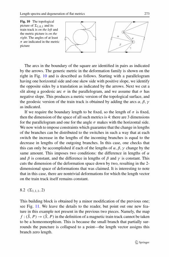
Length spectra and degeneration of flat metrics 273
Fig. 10 The topologicalpicture of �1,0,1 and itstrain track is on the left andthe metric picture is on theright. The angles of at leastπ are indicated in the metricpicture
The arcs in the boundary of the square are identified in pairs as indicatedby the arrows. The generic metric in the deformation family is shown on theright in Fig. 10 and is described as follows. Starting with a parallelogramhaving one horizontal side and one skew side with positive slope, we identifythe opposite sides by a translation as indicated by the arrows. Next we cut aslit along a geodesic arc σ in the parallelogram, and we assume that σ hasnegative slope. This produces a metric version of the topological surface, andthe geodesic version of the train track is obtained by adding the arcs α,β, γ
as indicated.If we require the boundary length to be fixed, so the length of σ is fixed,
then the dimension of the space of all such metrics is 4: there are 3 dimensionsfor the parallelogram and one for the angle σ makes with the horizontal side.We now wish to impose constraints which guarantee that the change in lengthsof the branches can be distributed to the switches in such a way that at eachswitch the increase in the lengths of the incoming branches is equal to thedecrease in lengths of the outgoing branches. In this case, one checks thatthis can only be accomplished if each of the lengths of α,β, γ change by thesame amount. This imposes two conditions: the difference in lengths of α
and β is constant, and the difference in lengths of β and γ is constant. Thiscuts the dimension of the deformation space down by two, resulting in the 2-dimensional space of deformations that was claimed. It is interesting to notethat in this case, there are nontrivial deformations for which the length vectoron the train track itself remains constant.
8.2 (�1,1,1,2)
This building block is obtained by a minor modification of the previous one;see Fig. 11. We leave the details to the reader, but point out one new fea-ture in this example not present in the previous two pieces. Namely, the mapf : (S,P ) → (S,P ) in the definition of a magnetic train track cannot be takento be a homeomorphism. This is because the small branch that partially sur-rounds the puncture is collapsed to a point—the length vector assigns thisbranch zero length.
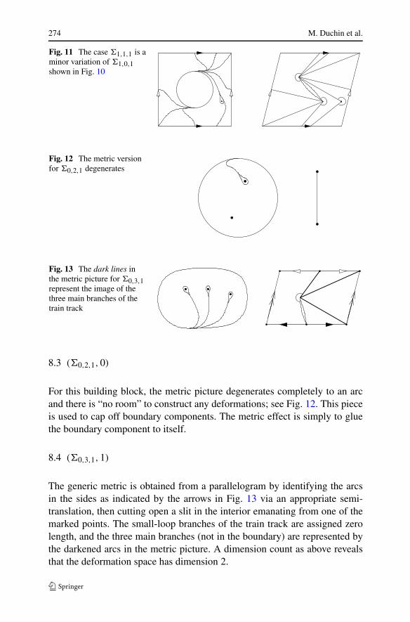
274 M. Duchin et al.
Fig. 11 The case �1,1,1 is aminor variation of �1,0,1shown in Fig. 10
Fig. 12 The metric versionfor �0,2,1 degenerates
Fig. 13 The dark lines inthe metric picture for �0,3,1represent the image of thethree main branches of thetrain track
8.3 (�0,2,1,0)
For this building block, the metric picture degenerates completely to an arcand there is “no room” to construct any deformations; see Fig. 12. This pieceis used to cap off boundary components. The metric effect is simply to gluethe boundary component to itself.
8.4 (�0,3,1,1)
The generic metric is obtained from a parallelogram by identifying the arcsin the sides as indicated by the arrows in Fig. 13 via an appropriate semi-translation, then cutting open a slit in the interior emanating from one of themarked points. The small-loop branches of the train track are assigned zerolength, and the three main branches (not in the boundary) are represented bythe darkened arcs in the metric picture. A dimension count as above revealsthat the deformation space has dimension 2.
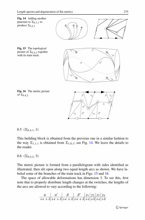
Length spectra and degeneration of flat metrics 275
Fig. 14 Adding anotherpuncture to �0,3,1 toproduce �0,4,1
Fig. 15 The topologicalpicture of �0,4,2 togetherwith its train track
Fig. 16 The metric pictureof �0,4,2
8.5 (�0,4,1,1)
This building block is obtained from the previous one in a similar fashion tothe way �1,1,1 is obtained from �1,0,1; see Fig. 14. We leave the details tothe reader.
8.6 (�0,4,2,3)
The metric picture is formed from a parallelogram with sides identified asillustrated, then slit open along two equal-length arcs as shown. We have la-beled some of the branches of the train track in Figs. 15 and 16.
The space of allowable deformations has dimension 3. To see this, firstnote that to properly distribute length changes at the switches, the lengths ofthe arcs are allowed to vary according to the following:
α α′ β β ′ γ1 γ2 γ3 γ4+ε + δ +ε + δ +ε + δ +ε + δ +ε +δ +ε +δ

276 M. Duchin et al.
To see that these variations are indeed possible (for small ε and δ), weagain appeal to a dimension count. The space of parallelograms with a pairof slits of fixed, equal length is 3 + 3 + 3 = 9 dimensions. The 9-dimensionalparameter space is subject to 6 equations derived from the geometry, leaving3 degrees of freedom.
References
1. Alperin, R., Bass, H.: Length functions of group actions on �-trees. In: CombinatorialGroup Theory and Topology, Alta, Utah, 1984. Ann. of Math. Stud., vol. 111, pp. 265–378. Princeton Univ. Press, Princeton (1987)
2. Birman, J.S., Series, C.: Geodesics with bounded intersection number on surfaces aresparsely distributed. Topology 24(2), 217–225 (1985)
3. Bonahon, F.: Bouts des variétés hyperboliques de dimension 3. Ann. Math. (2) 124(1),71–158 (1986)
4. Bonahon, F.: The geometry of Teichmüller space via geodesic currents. Invent. Math.92(1), 139–162 (1988)
5. Buser, P.: Geometry and Spectra of Compact Riemann Surfaces. Progress in Mathematics,vol. 106. Birkhäuser, Boston (1992)
6. Cohen, M.M., Lustig, M., Steiner, M.: R-tree actions are not determined by the translationlengths of finitely many elements. In: Arboreal Group Theory, Berkeley, CA, 1988. Math.Sci. Res. Inst. Publ., vol. 19, pp. 183–187. Springer, New York (1991)
7. Croke, C., Fathi, A., Feldman, J.: The marked length-spectrum of a surface of nonpositivecurvature. Topology 31(4), 847–855 (1992)
8. Croke, C.B.: Rigidity for surfaces of nonpositive curvature. Comment. Math. Helv. 65(1),150–169 (1990)
9. Culler, M., Morgan, J.W.: Group actions on R-trees. Proc. Lond. Math. Soc. (3) 55(3),571–604 (1987)
10. Fathi, A.: Le spectre marqué des longueurs des surfaces sans points conjugués. C. R. Acad.Sci. Paris Sér. I Math. 309(9), 621–624 (1989)
11. Fathi, A., Laudenbach, F., Poenaru, V.: Travaux de Thurston sur les Surfaces. Astérisque,vol. 66. Société Mathématique de France, Paris (1979). Séminaire Orsay, With an Englishsummary
12. Gardiner, F.P., Lakic, N.: Quasiconformal Teichmüller Theory. Mathematical Surveys andMonographs, vol. 76. American Mathematical Society, Providence (2000)
13. Gardiner, F.P., Masur, H.: Extremal length geometry of Teichmüller space. Complex Var.Theory Appl. 16(2–3), 209–237 (1991)
14. Hamenstädt, U.: Length functions and parameterizations of Teichmüller space for surfaceswith cusps. Ann. Acad. Sci. Fenn. Math. 28(1), 75–88 (2003)
15. Hamenstädt, U.: Parametrizations of Teichmüller space and its Thurston boundary. In:Geometric Analysis and Nonlinear Partial Differential Equations, pp. 81–88. Springer,Berlin (2003)
16. Hersonsky, S., Paulin, F.: On the rigidity of discrete isometry groups of negatively curvedspaces. Comment. Math. Helv. 72(3), 349–388 (1997)
17. Kerckhoff, S.P.: The asymptotic geometry of Teichmüller space. Topology 19(1), 23–41(1980)
18. Lenzhen, A.: Teichmüller geodesics that do not have a limit in PMF . Geom. Topol. 12(1),177–197 (2008)
19. Levitt, G.: Foliations and laminations on hyperbolic surfaces. Topology 22(2), 119–135(1983)

Length spectra and degeneration of flat metrics 277
20. Masur, H.: On a class of geodesics in Teichmüller space. Ann. Math. (2) 102(2), 205–221(1975)
21. Masur, H.: Closed trajectories for quadratic differentials with an application to billiards.Duke Math. J. 53(2), 307–314 (1986)
22. McMullen, C.: Amenability, Poincaré series and quasiconformal maps. Invent. Math.97(1), 95–127 (1989)
23. Nagata, J.: Modern Dimension Theory, revised edn. Sigma Series in Pure Mathematics,vol. 2. Heldermann Verlag, Berlin (1983)
24. Otal, J.P.: Le spectre marqué des longueurs des surfaces à courbure négative. Ann. Math.(2) 131(1), 151–162 (1990)
25. Papadopoulos, A. (ed.): Handbook of Teichmüller Theory. Vol. I. IRMA Lectures in Math-ematics and Theoretical Physics, vol. 11. European Mathematical Society (EMS), Zürich(2007)
26. Penner, R.C., Harer, J.L.: Combinatorics of Train Tracks. Annals of Mathematics Studies,vol. 125. Princeton University Press, Princeton (1992)
27. Rafi, K.: A characterization of short curves of a Teichmüller geodesic. Geom. Topol. 9,179–202 (2005)
28. Schmutz, P.: Die Parametrisierung des Teichmüllerraumes durch geodätische Längenfunk-tionen. Comment. Math. Helv. 68(2), 278–288 (1993)
29. Smillie, J., Vogtmann, K.: Length functions and outer space. Mich. Math. J. 39(3), 485–493 (1992)
30. Strebel, K.: Quadratic Differentials. A Series of Modern Surveys in Mathematics, vol. 5.Springer, Berlin (1980)
31. Sunada, T.: Riemannian coverings and isospectral manifolds. Ann. Math. (2) 121(1), 169–186 (1985)