Embed Size (px)
Citation preview

Lecture Notes on
String TheoryKevin Zhou
I should preface these notes by stating that I don’t actually know any string theory at all. These
“notes on string theory” are really just a collection of the prerequisites one needs to know before
starting to learn string theory, beyond the usual ones of quantum field theory and general relativity.
Topics covered include the quantization of constrained systems, 2D conformal field theory, and the
quantization of the bosonic string. Nothing in these notes is original; they have been compiled from
a variety of sources. The primary sources were:
• David Tong’s String Theory lecture notes. These clear lecture notes follow the first volume of
Polchinski, but with a much more approachable style, and hence are accessible after a good
course on quantum field theory.
• Timo Weigand’s String Theory lecture notes. As with the quantum field theory notes, these
notes are slightly more comprehensive and precise, at the cost of being slightly drier; also
contains a short introduction to the superstring.
• Zwiebach, A First Course in String Theory. A very basic introduction, covering bosonic string
theory in the first part, and a wide variety of developments, such as D-branes and AdS/CFT in
the second. The book is clearly written and accessible even without any field theory background,
and in fact might be useful as indirect preparation for field theory. It has the benefit of explicitly
showing many steps of logic skipped in most books. The downside is that the entire 300 pages
of the first part barely covers the first 30 pages of Polchinski.
• Henneaux and Teitelboim, Quantization of Gauge Systems. The most thorough book by far on
the subject; if you’re wondering how constrained quantization, Grassmann variables, or BRST
symmetry really work, this is the place to go. Naturally, more formal than any of the other
books on this list. The most relevant chapters for these notes are 1, 4, 6, and 13.
The most recent version is here; please report any errors found to [email protected].
1 Contents
Contents
1 Preliminaries 2
1.1 Miscellanea . . . . . . . . . . . . . . . . . . . . . . . . . . . . . . . . . . . . . . . . . 2
1.2 Classical Strings . . . . . . . . . . . . . . . . . . . . . . . . . . . . . . . . . . . . . . 5
1.3 String Motion . . . . . . . . . . . . . . . . . . . . . . . . . . . . . . . . . . . . . . . . 10
1.4 Light Cone Gauge . . . . . . . . . . . . . . . . . . . . . . . . . . . . . . . . . . . . . 14
1.5 Light Cone Fields . . . . . . . . . . . . . . . . . . . . . . . . . . . . . . . . . . . . . . 19
1.6 The Veneziano Amplitude . . . . . . . . . . . . . . . . . . . . . . . . . . . . . . . . . 22
2 Constrained Systems 25
2.1 Constrained Hamiltonian Systems . . . . . . . . . . . . . . . . . . . . . . . . . . . . 25
2.2 Dirac Brackets and Gauge Fixing . . . . . . . . . . . . . . . . . . . . . . . . . . . . . 28
2.3 General Covariance . . . . . . . . . . . . . . . . . . . . . . . . . . . . . . . . . . . . . 31
2.4 Constrained Quantization . . . . . . . . . . . . . . . . . . . . . . . . . . . . . . . . . 33
2.5 Classical Point Particle . . . . . . . . . . . . . . . . . . . . . . . . . . . . . . . . . . . 36
3 The Bosonic String 41
3.1 The Polyakov Action . . . . . . . . . . . . . . . . . . . . . . . . . . . . . . . . . . . . 41
3.2 Old Covariant Quantization . . . . . . . . . . . . . . . . . . . . . . . . . . . . . . . . 46
3.3 Computing Spectra . . . . . . . . . . . . . . . . . . . . . . . . . . . . . . . . . . . . . 51
4 Conformal Field Theory 56
4.1 Conformal Transformations . . . . . . . . . . . . . . . . . . . . . . . . . . . . . . . . 56
4.2 Elementary Aspects . . . . . . . . . . . . . . . . . . . . . . . . . . . . . . . . . . . . 59
4.3 Free Scalar Field . . . . . . . . . . . . . . . . . . . . . . . . . . . . . . . . . . . . . . 64
4.4 Central Charges . . . . . . . . . . . . . . . . . . . . . . . . . . . . . . . . . . . . . . 67
4.5 The Virasoro Algebra . . . . . . . . . . . . . . . . . . . . . . . . . . . . . . . . . . . 71
4.6 The State-Operator Correspondence . . . . . . . . . . . . . . . . . . . . . . . . . . . 74
5 String Interactions 79
5.1 Motivation . . . . . . . . . . . . . . . . . . . . . . . . . . . . . . . . . . . . . . . . . 79
5.2 Vertex Operators . . . . . . . . . . . . . . . . . . . . . . . . . . . . . . . . . . . . . . 83
5.3 Bosonic Open Strings . . . . . . . . . . . . . . . . . . . . . . . . . . . . . . . . . . . 85
6 String Compactification 89
6.1 Kaluza–Klein Theory . . . . . . . . . . . . . . . . . . . . . . . . . . . . . . . . . . . . 89
6.2 Worldsheet Theory . . . . . . . . . . . . . . . . . . . . . . . . . . . . . . . . . . . . . 90
2 1. Preliminaries
1 Preliminaries
1.1 Miscellanea
As a first pass, we’ll follow Zwiebach’s text. In this first section, we establish some conventions.
• There are three fundamental dimensions: mass, length, and time. Charge is not a independent
dimension; this is clearest in the cgs system, where the Coulomb force law is F = q1q2/r2. That
is, one can define charges purely in terms of the forces they produce. In the SI system, all
occurrences of the unit of charge in measurable quantities are canceled out by ε0 or µ0.
• String theory is said to have no adjustable parameters. This means that it has no dimensionless
parameters; there is a single dimensionful parameter, the string length `s. When string theory
was considered as a theory of hadrons, `s was thought to be on the nuclear scale, but now it is
viewed as much smaller.
• We use the (−+ ++) metric convention, but define the interval ds2 to measure proper time,
−ds2 = ηµνdxµdxν .
• We will perform the quantization of the relativistic string in light cone coordinates, where
x± =1√2
(x0 ± x1).
The other coordinates stay the same, so in xµ, the µ index runs over (+,−, 2, 3). The light
cone coordinate axes are tilted so that they lie on the light cone, e.g. a photon moving to the
right has x− = 0.
• The metric in light cone coordinates is
−ds2 = −2dx+dx− + (dx2)2 + (dx3)2, ηµν =
−1
−1
1
1
.
For example, we have
a+ = −a−, a− = −a+, aµbµ = −a−b+ − a+b− + a2b2 + a3b3.
• None of the coordinates are true time coordinates, but we will conventionally think of x+ as
the light cone time coordinate. This isn’t completely unnatural, since dx±/dτ > 0 for almost
all particles.
• We think of dx−/dx+ as a “light cone velocity”. For a particle with speed v, the light cone
velocity is (1− v)/(1 + v). In particular, it is zero for a massless particle moving to the right,
infinite for a massless particle moving to the left, and one when v = 0.
• Next we must define the light cone energy. Energy is the conjugate variable to time, and
pµxµ = p+x
+ + p−x− + p2x
2 + p3x3
which motivates us to define the light cone energy as −p+ = p−. Defining energy as a conjugate
variable is useful as, e.g. the Schrodinger equation i ∂ψ/∂x0 = p0ψ becomes i ∂ψ/∂x+ = p−ψ
in lightcone coordinates.
3 1. Preliminaries
Next, we consider the possibility of extra spatial dimensions. We maintain only one time dimension,
since it is difficult to construct a consistent theory with more than one.
• The extra dimensions can be topologically nontrivial; for example, for a single dimension we
may identify x ∼ x + 2πR. The interval 0 ≤ x < 2πR is a fundamental domain for this
identification, as every point is identified with exactly one point in the fundamental domain.
We then construct the space by identifying points on the boundary, getting a circle.
• Sometimes identifications have fixed points. The resulting space is not a manifold, since it is
singular at the fixed point, but an orbifold. For example, identifying x ∼ −x gives the half-line
x ≥ 0, called the R1/Z2 orbifold.
• As another example, consider the identification z ∼ e2πi/Nz in the complex plane, giving
the C/ZN orbifold. It is a cone which is singular at its vertex; one fundamental domain is
0 ≤ θ < 2π/N .
• Physics on spaces with generic singularities is typically complicated and possibly even inconsis-
tent. Orbifolds are interesting because they have “tractable” singularities, so we may quantize
strings on them.
• For point particles, a small compactified dimension creates new energy levels, but they are very
high if the dimension is small. By contrast, for a string, new low-lying states can appear if the
dimension is much smaller than the string length, corresponding to the string wrapping around
it. This is a consequence of T duality, as we’ll see.
• Compactified dimensions lead to subtleties with gauge theory. It can be the case that two
configurations with the same fields are not related by a gauge transformation; then we must
consider the states physically distinct. It also also be the case that some configuration of fields
cannot be realized by a potential, even if we allow the potential be defined on patches and
related between patches with gauge transformations; such states are forbidden.
Note. A quick review of the nonrelativistic string. The Lagrangian is
L =1
2µ
(∂y
∂t
)2
− 1
2T
(∂y
∂x
)2
.
When we attempt to extremize the action, we run into a boundary term
δS ⊃ −T∫dt
(∂y
∂xδy
) ∣∣∣∣x=a
x=0
.
To remove this unwanted boundary term, we need to apply boundary conditions. One acceptable
boundary condition is Neumann boundary conditions (free ends), where
∂y
∂x
∣∣∣∣x=0,a
= 0.
Alternatively, we could use Dirichlet boundary conditions (fixed ends),
∂y
∂t
∣∣∣∣x=0,a
= 0

4 1. Preliminaries
which ensures that y is constant on the boundaries, and hence δy = 0 there. A third alternative is
that the string is closed, so that there are no boundaries at all.
In the initial days of string theory, open strings were given Neumann boundary conditions, but
it was later realized that they could have Dirichlet boundary conditions if they attached to an
extended object called a Dp-brane, where D stands for Dirichlet and p is the number of spatial
dimensions. (One can think of Neumann boundary conditions as the special case where the D-brane
fills all space.) Remarkably, it turns out that D-branes are physical objects in their own right, and
arise naturally from string theory without being introduced by hand.
Finally, it will be useful later to consider the conjugate momenta,
Pt =∂L∂y
= µ∂y
∂t, Px =
∂L∂y′
= −T ∂y∂x.
Here Pt is simply the usual momentum density in the y-direction. The equation of motion is
∂Pt
∂t+∂Px
∂x= 0.
In this notation, Neumann and Dirichlet boundary conditions set Px = 0 and Pt = 0 respectively.
Note. Gravity and electromagnetism in higher dimensions. We will use
vol(Sd−1) =2πd/2
Γ(d/2), vol(Bd) =
πd/2
Γ(1 + d/2).
In d spatial dimensions, Gauss’s law continues to hold, so the field of a point charge is
E(r) =1
vol(Sd−1)
q
rd−1
in cgs units. As for gravitation, we have
g(r) =Gm
r2
in D = 4 spacetime dimensions. More generally, the gravitational field is determined by
∇2V (D) = 4πG(D)ρ, g = −∇V
where G(D) is the gravitational constant in D dimensions. The Planck length in D dimensions is
related by dimensional analysis,
~c3
=`2PG
=(`
(D)P )D−2
G(D).
In order to relate gravitational constants in different dimensions, we need to relate densities in
different dimensions. Consider a single small compactified dimension of length `C . Then for distances
much greater than `C we have the coarse-grained mass density
ρ(4) = 2πRρ(5).
Plugging this into Poisson’s equation, we conclude
G(5)
G= `C
5 1. Preliminaries
and more generally for multiple compactified dimensions with volume VC ,
G(D)
G= VC .
For a D-dimensional theory where each compactified dimension has length `C ,
(`(D)P )D−2 = (`P )2G
(D)
G= (`P )2(`C)D−4, `C = `
(D)P
(`(D)P
`P
) 2D−4
.
Intuitively, in the presence of compactified dimensions, gravity appears much weaker than it actually
is, leading to an underestimate of the fundamental Planck length `(D)P . In particular, for two
compactified dimensions (D = 6) we could have a TeV-scale Planck energy if `C ∼ 10−5 m.
In the context of string theory, the macroscopic dimensions form a D3-brane; open strings
must terminate on this brane while closed strings do not. Electromagnetism and other forces are
associated with open strings and hence are not affected by the extra dimensions, while gravity is
associated with closed strings. Then the hypothesis of large extra dimensions could only be tested
by measuring gravitational effects at short distances, which is extremely difficult. It predicts the
appearance of many new, stringy excitations at a scale much lower than the conventional Planck
scale.
Note. The study of higher dimensions began with Kaluza–Klein theory, which is essentially general
relativity in five dimensions. Upon compactifying the fifth dimension, and restricting to four
dimensions, the metric tensor gMN (with M,N = 0, . . . , 4) decomposes into the ordinary metric
gµν , a massless vector field gµ4 interpreted as the electromagnetic field, and a massless scalar field
g44. This scalar field was originally thought to be problematic, but was later incorporated into
Brans–Dicke theory, an extension of general relativity. In string theory, the dilaton plays a similar
role.
1.2 Classical Strings
We now arrive at the classical relativistic string.
• A relativistic string traces out a two-dimensional surface in spacetime, called a worldsheet. The
Nambu–Goto action is the area of the worldsheet.
• As a warmup, consider a surface in space, parametrized as x(ξ1, ξ2). Since the area spanned
by two vectors is the determinant of the 2× 2 matrix that contains them,
A =
∫dξ1dξ2
√(∂1x · ∂1x)(∂2x · ∂2x)− (∂1x · ∂2x)2
where ∂i is a derivative with respect to ξi.
• It is simpler to express this in terms of the induced metric on the worldsheet,
ds2 = gij dξidξj , gij = ∂ix · ∂jx.
This is the metric in the (ξ1, ξ2) coordinates, and the area is
A =
∫dξ1dξ2√g
which is manifestly reparametrization invariant.

6 1. Preliminaries
• Now, for a spacetime surface, we parametrize the worldsheet as Xµ(τ, σ). Note that conven-
tionally one calls both the domain and image of this map the worldsheet, though we will stick
to the latter usage. The letter X is capitalized to avoid confusing the string coordinates Xµ
with spacetime coordinates xµ.
• The parameter τ is roughly related to time on the string, while σ is roughly related to position
along the string. As such, we define
X =∂X
∂τ, X ′ =
∂X
∂σ
and we require X0 6= 0. We will usually choose X ′ to be spacelike and X to be timelike or null.
It is tempting to identify X with the velocity of a piece of the string, but this is inappropriate
as none of the points on the string are distinguishable.
• By analogy with the spatial case, the area is
A =
∫dτdσ
√(X ·X ′)2 − (X)2(X ′)2.
This is an area in Lorentzian signature, which is somewhat less intuitive. There is a minus sign
relative to the spatial case so the argument of the square root is positive, and the area is zero
if the string is moving transverse to itself at the speed of light.
• The Nambu–Goto action is
S = −T0
∫ τf
τi
dτ
∫ σ1
0dσ
√(X ·X ′)2 − (X)2(X ′)2
where T0 is called the string tension. The easiest way to check reparametrization invariance is
again to introduce a metric on the worldsheet,
−ds2 = ηµνdXµdxν = γαβdξ
αdξβ, γαβ =∂X
∂ξα· ∂X∂ξβ
=
(X2 X ·X ′
X ·X ′ (X ′)2
).
Then the Nambu–Goto action can be written in the manifestly reparametrization invariant
form
S = −T0
∫dτdσ
√−γ.
Now we turn to the equations of motion.
• Writing the Nambu–Goto action as the integral of a Lagrangian density as usual, we define the
canonical momenta
P τµ =∂L∂Xµ
= −T0
(X ·X ′)X ′µ − (X ′)2Xµ√(X ·X ′)2 − (X)2(X ′)2
, P σµ =∂L∂X ′µ
= −T0
(X ·X ′)Xµ − (X)2X ′µ√(X ·X ′)2 − (X)2(X ′)2
.
Throwing away boundary terms, the Euler-Lagrange equation is
∂P τµ∂τ
+∂P σµ∂σ
= 0
which is quite complicated in terms of X and X ′.
7 1. Preliminaries
• As for the nonrelativistic string, the derivation only goes through if we can ignore boundary
terms. The τ boundary terms vanish by fixing the initial condition Xµ(τi, σ) and final condition
Xµ(τf , σ), leaving the σ boundary term,
δS ⊃∫dτ (δXµ P σµ )
∣∣∣∣σ10
.
• In the case of a closed string, these conditions are automatically satisfied by the periodicity of
Xµ. For an open string, we may remove these terms by imposing Dirichlet boundary conditions,
∂Xµ
∂τ
∣∣∣∣σ=σ∗
or the free endpoint condition,
P σµ
∣∣∣∣σ=σ∗
= 0.
The Dirichlet boundary condition cannot be used for µ = 0, so we must use the free endpoint
condition there. The free endpoint condition is analogous to a Neumann boundary condition.
We will show later that the Dirichlet boundary condition implies P τµ = 0 at the string endpoints.
• In order to simplify the equations, we work in the static gauge, where
τ = t
where t is the time coordinate. This is called the static gauge because constant τ slices match
constant t slices. We normalize σ by
σ ∈ [0, σ1] for open string, σ ∈ [0, σc] for closed string.
In the static gauge we simply have
X ′ =
(0,∂X
∂σ
), X =
(1,∂X
∂t
).
Example. A stretched string. Suppose a string is static along the x1 axis, with endpoints at x1 = 0
and x1 = a. Then X1(f, σ) = f(σ), and we have
(X ′)1 = f ′(σ), (X)0 = 1
with all other elements zero. Note that f(σ) must assign every point on the string a unique parameter
value, so f ′(σ) > 0. The action is simply
S = −T0
∫dt
∫dσ√f ′2 = −T0a
∫ tf
ti
dt.
Since generically L = T − V and the kinetic energy vanishes here, this may be interpreted as a
potential T0a, justifying the interpretation of T0 as a tension. The equation of motion is
∂P σµ∂σ
= 0, P σµ = −T0
X ′µf ′
Then P σµ = −T0δµ1 and hence the equation of motion is satisfied.
8 1. Preliminaries
The longitudinal velocity of a string is not meaningful, but we can get further insight by writing
the action in terms of transverse velocity.
• Let s measure length along the string, so that ∂X/∂s is a spatial unit vector. We then project
out the longitudinal part of the string velocity ∂X/∂t, defining
v⊥ =∂X
∂t−(∂X
∂t· ∂X
∂s
)∂X
∂s, v2
⊥ =
(∂X
∂t
)2
−(∂X
∂t· ∂X
∂s
)2
.
The Nambu–Goto action can then simply be written as
S = −T0
∫dt
∫ds√
1− v2⊥.
• This is closely analogous to the relativistic point particle action. To make the analogy even
clearer, we imagine a string as starting with an infinitesimal length. It takes work T0a to stretch
it to a length a, which gives it a mass T0a. Hence T0 is the mass per length of the string.
• A somewhat nasty calculation shows that
P σµ = − T0√1− v2
⊥
((∂X
∂s· ∂X
∂t
)Xµ +
(1−
(∂X
∂t
)2)∂Xµ
∂s
)
as well as
P σ0 = −T0
(∂X∂s ·
∂X∂t
)√1− v2
⊥
, P τ0 = T0ds
dσ
1√1− v2
⊥
, P τi = T0ds
dσ
vi⊥√1− v2
⊥
.
• Now consider the motion of the endpoints of an open string; these are distinguished points and
hence have an unambiguous velocity. At the endpoints, P σµ must vanish, and hence for P σ0 to
vanish we must have (∂X/∂s) · (∂X/∂t) = 0. Then the string endpoints move transverse to the
string. Plugging this back into the general expression for P σµ, we see that (∂X/∂t)2 = 1, so
the endpoints move at the speed of light.
• Finally, by writing the Lagrangian as a function of ∂sX and ∂tX and performing a Legendre
transformation with respect to the canonical momentum P = ∂L/∂(∂tX), we find
H =
∫T0 ds√1− v2
⊥
which is precisely the kinetic energy of the string, with rest mass T0 per unit length. Similarly,
integrating P τi gives the momentum. Note that the speed of waves on a string is v =√T0/ρ
where ρ is the mass density, so excitations on the string travel at the speed of light.
Now we choose a useful parametrization for σ.
• One could replace the parameter σ with s, but it is more convenient to use a parameter with
a fixed range. Note that in static gauge, the spatial configuration of a string is described by
X(σ, t). This yields a two-dimensional spatial surface, which we’ll call the string surface; this
should not be confused with the worldsheet.
9 1. Preliminaries
• We know that ∂X/∂t is a unit vector on the string surface, so we choose σ so that
∂X
∂σ· ∂X
∂t= 0, v⊥ =
∂X
∂t.
Since s and σ are related to a scaling, we also have (∂X/∂s) · (∂X/∂t) = 0.
• As a result, our expressions for the momenta simplify,
P τµ = T0ds
dσ
∂Xµ/∂t√1− v2
⊥
, P σµ = −T0
√1− v2
⊥∂Xµ
∂s.
In other words, the simplifications that we previously found held for the string endpoints hold
everywhere on the string for this parametrization.
• Now we consider the equations of motion again. The µ = 0 component of the equation of
motion is simply∂P τ0
∂t= 0.
However, P τ0 is simply the energy density of the string, per unit σ. The conservation of this
quantity makes sense because, unlike strings that actually exist, the string motion here is purely
transverse, so the tension does zero work on any segment with endpoints of fixed σ. If the
transverse speed of such a segment changes, the energy comes from the individual stretching
or shrinking of that segment.
• The spatial components of the equation of motion read
∂
∂σ
(T0
√1− v2
⊥∂X
∂s
)= T0
ds/dσ√1− v2
⊥
∂v⊥∂t
which rearranges toT0√
1− v2⊥
∂v⊥∂t
=∂
∂s
(T0
√1− v2
⊥∂X
∂s
).
This is precisely the usual wave equation, if we interpret T0 as the tension in the rest frame
of a piece of string. Then the factor of√
1− v2⊥ on the right simply reflects the Lorentz
transformation of force, while the factor of γ on the left reflects the fact that moving objects
are harder to turn by a factor of γ.
• This also physically explains why the endpoints of an open string must move at the speed of
light. The tension on a real open string goes to zero at endpoints because the endpoints have
no mass and hence can experience no force. But the proper tension in these abstract strings is
constant, so we only avoid a divergence if it Lorentz transforms to zero at the ends.
• We have still not used up all the freedom in σ parametrization. We already know that the
energy of a piece of string whose endpoints have fixed σ is constant. Hence it is consistent to
scale σ so the energy density is constant,
dσ =ds√
1− v2⊥
=dE
T0.
10 1. Preliminaries
Then we have σ ∈ [0, σ1] where σ1 = E/T0. This is equivalent to(∂X
∂σ
)2
+
(∂X
∂t
)2
= 1.
• In this case, the equation of motion reduces to
∂2X
∂t2=∂2X
∂σ2.
The canonical momenta and boundary conditions are now
P τµ = T0∂Xµ
∂t, P σµ = −T0
∂Xµ
∂σ,
∂X
∂σ= 0 at endpoints.
Note that we no longer have 1/√
1− v2⊥ Lorentz factors, because we’re now parametrizing by
energy rather than by length.
Note. As shown in the lecture notes on General Relativity, energy density and pressure contribute
equally to gravitational attraction. A string has a negative pressure due to its tension, which is
equal to its mass density, so a long static string would exert no gravitational force. Cosmic strings
would instead be detected by the deficit angles they produce, which would yield multiple images of
distant objects.
1.3 String Motion
With the wave equation, we may now solve for the general motion of open and closed strings.
• A solution to the wave equation can always be written as a superposition of “left moving” and
“right moving” solutions,
X(t, σ) =1
2(F(t+ σ) + G(t− σ)).
The boundary condition at the σ = 0 endpoint demands that F′ = G′, so they differ by a
constant. Hence the general solution can be written as
X(t, σ) =1
2(F(t+ σ) + F(t− σ)).
• Next, consider the boundary condition at σ = σ1, which gives
F′(t+ σ1) = F′(t− σ1).
This implies that F is quasi-periodic,
F(u+ 2σ1) = F(u) + 2σ1v0.
To interpret F, note that X(t, 0) = F(t), so the curve F(u) traces out the motion of the σ = 0
endpoint, and v0 is its average speed.
11 1. Preliminaries
• By adding and subtracting the results(∂X
∂σ
)2
+
(∂X
∂t
)2
= 1,∂X
∂σ· ∂X
∂t= 0
we have the equivalent set of two constraints(∂X
∂σ± ∂X
∂t
)2
= 1.
Plugging this into our general form shows that∣∣∣∣dFdu∣∣∣∣2 = 1
so that u can be interpreted as a length parameter along the curve F(u). This constraint is
equivalent to demanding the endpoint σ = 0 moves at the speed of light.
• We now consider the motion of a closed string. This is a bit more complicated because we can’t
use boundary conditions to eliminate G. We start with the general solution
X(t, σ) =1
2(F(u) + G(v)), u = t+ σ, v = t− σ.
We may solve for the derivatives of F and G in terms of X,
∂X
∂σ+∂X
∂t= F′(u),
∂X
∂σ− ∂X
∂t= −G′(v).
As a result, the parametrization constraints give∣∣∣∣dFdu∣∣∣∣2 =
∣∣∣∣dGdv∣∣∣∣2 = 1.
• Instead of a boundary condition, we have a periodicity condition σ ∼ σ+ σ1, which means that
X(t, σ + σ1) = X(t, σ). This is equivalent to
F(u+ σ1)− F(u) = G(v)−G(v − σ1).
That is, both F and G are quasi-periodic with the same constant.
• One interesting generic phenomenon is the formation of cusps. Note that F′ and G′ are periodic
functions on the unit sphere. Suppose that F′(u0) = G′(v0), with corresponding coordinates
(t0, σ0). Without loss of generality, we shift to set t0 = σ0 = 0 and hence u0 = v0 = 0.
• Now we Taylor expand the shape of the string about this point,
X(0, σ)−X(0, 0) = σ∂X
∂σ+σ2
2
∂2X
∂σ2+ . . . .
We note that∂X
∂σ=
1
2(F′ −G′) = 0.
Therefore, the leading term is quadratic, which means we have a cusp; the string enters in
one direction and exits along the same direction. Generically cusps will appear and disappear
periodically throughout the string. They are thought to be efficient sources of gravitational
waves for cosmic strings.
12 1. Preliminaries
Example. Consider a straight string of length ` rotating with angular velocity ω, with its midpoint
at the origin of the xy plane. We can infer F(u) from the endpoint motion,
F(u) =`
2(cosωu, sinωu).
Periodicity requires ω = πm/σ1 for an integer m, and
X(0, σ) =F(σ) + F(−σ)
2=`
2(cos(πmσ/σ1), 0).
For m > 1, the string traces over itself multiple times, so we focus on the case m = 1. Since the
σ = 0 endpoint moves at the speed of light,
` =2
ω=
2σ1
π=
2
π
E
T0
so the total energy is (π/2)T0`. The tension provides T0`, while the rest is due to the kinetic energy
of the string. The complete solution as a function of time is
X(t, σ) =σ1
πcos
πσ
σ1
(cos
πt
σ1, sin
πt
σ1
).
We now apply Noether’s theorem to find conserved quantities.
• The results of Noether’s theorem will look somewhat different. Usually, a classical field maps
from spacetime, φ : R4 → N where N is the field space. However, in string theory we deal with
maps into spacetime, Xµ : M → R4 where M is the worldsheet. Hence the dynamics of a single
string can be thought of as a two-dimensional field theory with a four-component field X.
• The action is
S =
∫dξi L(∂iX
µ), (ξ0, ξ1) = (τ, σ).
The fields Xµ have a continuous shift symmetry δXµ = εµ, which corresponds to translation in
spacetime. Applying Noether’s theorem, the conserved currents are
jαµ =∂L
∂(∂αXµ)= Pαµ .
These are simply the canonical momenta we defined earlier.
• The equation for current conservation is
∂αPαµ =
∂P τµ∂τ
+∂P σµ∂σ
= 0.
We know this holds on-shell, since it is precisely the equation of motion.
• The four conserved charges are found by integrating over “space” (i.e. σ) on the worldsheet,
pµ =
∫ σ1
0P τµ (τ, σ) dσ,
dpµdτ
= 0.

13 1. Preliminaries
To check conservation, note that
dpµdτ
=
∫ σ1
0
∂P τµ∂τ
dσ = −∫ σ1
0
∂P σµ∂σ
dσ = −P σµ∣∣∣∣σ10
.
The right-hand side vanishes for closed strings and open strings with free endpoints. For
open strings with Dirichlet boundary conditions, pµ is not conserved, reflecting the fact that
momentum can be transferred to the D-brane.
• Since pµ it is associated with spacetime translation of the string, we expect it is the total
energy-momentum of the string, and indeed in the static gauge τ = t we have dpµ/dt = 0 and
pµ is the total energy-momentum of the string, as we argued above. Since εµ is a vector, the
index on pµ is a vector index, so it transforms as expected under Lorentz transformations.
• To interpret pµ for a general parametrization, we simply note that Noether charges Q =∫
Σ(n ·j)are scalars which are independent of the surface Σ used to compute them, a fact proven in the
lecture notes on General Relativity. Hence pµ is always the conserved energy-momentum, in
any parametrization. Furthermore, we need not compute it over a curve of constant τ . For an
arbitrary curve γ, which is only required to wrap around the worldsheet once for a closed string
or end at the endpoints for an open string, we have
pµ =
∫γPµ · dn =
∫γP τµ dσ − P σµ dτ.
The relative sign is just because the normal to (dτ, dσ) is dn = (dσ,−dτ).
Next, we turn to Lorentz symmetry.
• As usual, Lorentz symmetry is generated by
δXµ = εµνXν , εµν = −ενµ.
The string Lagrangian contains terms of the form ηµν(∂Xµ/∂ξα)(∂Xν/∂ξβ). Since Xµ is a
Lorentz vector and ξ is a Lorentz scalar, the two quantities in parentheses are Lorentz vectors,
so the string Lagrangian is a Lorentz scalar as expected.
• Applying Noether’s theorem, the conserved currents can be packaged into a Lorentz tensor,
Mαµν = XµP
αν −XνP
αµ .
The conserved charges can be computed similarly,
Mµν =
∫γMτ
µν dσ −Mσµν dτ.
As usual, these Lorentz tensors are antisymmetric. As with the momenta, these charges might
not be conserved for an open string attached to a D-brane.
• Explicitly, integrating over a curve γ with constant τ ,
Mµν =
∫XµP
τν −XνP
τµ dσ
14 1. Preliminaries
and the charges associated with boosts are
M0i =
∫tP τi −XiP τ0 dσ = tpi −XCME
where XCM is the spatial center of mass of the string, and conservation of M0i ensures the
center of mass moves at a constant velocity.
Example. Consider the rotating string of the previous example. We have
Pτ = T0∂X
∂t= T0 cos
πσ
σ1
(− sin
πt
σ1, cos
πt
σ1
).
The angular momentum is
J = M12 =
∫ σ1
0X1P
τ2 −X2P
τ1 dσ =
σ1T0
π
∫ σ1
0cos2 πσ
σ1dσ =
σ21T0
2π.
Finally, using σ1 = E/T0 we have the relation
J
~= α′E2, α′ =
1
2πT0~c
where we restored ~ and c. Here α′ is called the slope parameter, and was important in ancient times
when string theory was used to predict the masses of mesons, which lied on “Regge trajectories”
with slope α′. The relation J ∼ E2 is quite unusual, and comes from the fact that the mass of a
string scales with its length. Given α′, we may also define a length scale
`s = ~c√α′
called the string length. Most modern work on string theory uses `s or α′, rather than T0. Originally,
`s ∼ 10−15 m to describe mesons, but this was invalidated by deep inelastic scattering experiments,
which instead supported QCD. In the modern usage of string theory as a theory of quantum gravity,
`s is around the Planck length.
1.4 Light Cone Gauge
We now introduce light cone gauge, which will be used to carry out the quantization of the string.
• Previously, we worked in static gauge, X0(τ, σ) = τ . We now consider the more general gauge
nµXµ(τ, σ) = λτ
for a constant vector nµ, which reduces to static gauge for nµ = (1, 0, 0, 0) and λ = 1. In this
gauge, the configuration of the string at worldsheet time τ is the intersection of the worldsheet
and a hyperplane orthogonal to nµ. To ensure this configuration is everywhere spacelike or null,
we restrict nµ to be spacelike or null.
• Like static gauge, this gauge is not Lorentz covariant. In a more advanced treatment, string
quantization would be carried out in a Lorentz covariant gauge, but the choice made here will
be simpler to understand.
15 1. Preliminaries
• Restricting to open strings, we recall that the string momentum pµ is conserved for free boundary
conditions, as P σ vanishes at the endpoints. For Dirichlet boundary conditions, n·p is conserved
as long as n · P σ vanishes at the endpoints, a weaker condition which we will assume holds.
• In either case, n · p is conserved, and we conventionally normalize τ to be dimensionless, with
n ·X = 2α′(n · p)τ.
Since both sides are proportional to n, the gauge no longer depends on the normalization of n.
To check the dimensions work out, note that [X] = −1, [p] = 1, [τ ] = 0, and [α′] = −2.
• Previously, we parametrized σ so that the energy density P τ0 was constant. This is generalized
to demanding the energy-momentum density n · P τ in the n direction is constant. Scaling so
that σ ∈ [0, π] for open strings, this means
n · P τ =n · pπ
.
That is, the left-hand side does not depend on σ or τ .
• Dotting both sides of the equation of motion with nµ, we find
∂
∂τ(n · P τ ) +
∂
∂σ(n · P σ) =
∂
∂σ(n · P σ) = 0
However, by assumption n · P σ = 0 at the endpoints, and hence
n · P σ = 0
everywhere on the string.
• For closed strings, the momentum p is conserved in all cases, so the same reasoning as above
goes through, with slightly different conventions,
n ·X = α′(n · p)τ, σ ∈ [0, 2π], n · P τ =n · p2π
.
Since there are no endpoints, it is ambiguous where σ = 0 is; furthermore we cannot use the
endpoints to show n · P σ = 0. These two problems may be solved simultaneously by choosing
the curve σ = 0 so that n · P σ = 0 on it.
• More explicitly, using the explicit expression for P σ we have
n · P σ ∝ (X ·X ′)∂τ (n ·X)− (X2)∂σ(n ·X) = (X ·X ′)∂τ (n ·X) ∝ X ·X ′.
Hence picking n · P σ = 0 is equivalent to setting X · X ′ = 0. This generalizes the condition
X ·X′ = 0 we imposed in static gauge, as there we had (X0)′ = 0.
We now turn to the associated constraints and wave equations.
• Using X ·X ′ = 0, the expression for P τ simplifies to
P τµ =1
2πα′X ′2Xµ√−X2X ′2
.
16 1. Preliminaries
Dotting n into both sides and applying the gauge condition, we have
1 =X ′2√−X2X ′2
for both open and closed strings, and using X ′2 > 0 we have
X2 +X ′2 = 0
which generalizes the normalization condition (∂X/∂σ)2 + (∂X/∂t)2 = 1 in static gauge. These
results together imply the induced metric on the worldsheet is conformally equivalent to the
flat metric, so this gauge is also called conformal gauge.
• Using this result, the expressions for the momenta simplify considerably,
P τµ =Xµ
2πα′, P σµ = − X
µ′
2πα′.
The equation of motion are simply wave equations,
Xµ −Xµ′′ = 0.
• Finally, adding and subtracting 2X ·X ′ = 0, our two constraints are equivalent to
(X ±X ′)2 = 0.
For an open string with free endpoints, we have the further constraint P σµ = 0 at the endpoints,
so Xµ′ vanishes at the endpoints.
We will now find the general solution for the open string motion, going further than in static gauge.
• Now consider an open string with free endpoints. The general solution of the wave equation is
Xµ(τ, σ) =1
2(fµ(τ + σ) + gµ(τ − σ)).
The constraint X ′ = 0 at σ = 0 yields fµ′ = gµ′, so the two differ by a constant, which can be
absorbed in a redefinition of fµ. Hence
Xµ(τ, σ) =1
2(fµ(τ + σ) + fµ(τ − σ)).
• The constraint X ′ = 0 at σ = π yields
fµ′(τ + π)− fµ′(τ − π) = 0
which shows that fµ′ is periodic with period 2π, justifying our earlier normalization convention.
• So far, this is familiar from static gauge; we now go further by expanding fµ′ in a Fourier series,
fµ′(u) = fµ1 +∑n>0
aµn cosnu+ bµn sinnu
which integrates to
fµ(u) = fµ0 + ufµ1 +∑n>0
Aµn cosnu+Bµn sinnu
and gives a general solution of
Xµ(τ, σ) = fµ0 + fµ1 τ +∑n>0
(Aµn cosnτ +Bµn sinnτ) cosnσ.
17 1. Preliminaries
• It is useful to change variables to
Aµn cosnτ +Bµn sinnτ = −i
√2α′√n
(aµn∗einτ − aµne−inτ )
so that the aµn are dimensionless; it will turn into an annihilation operator upon quantization.
Moreover, since the momentum density is
P τµ =1
2πα′Xµ =
1
2πα′fµ1 + oscillatory terms
we have fµ1 = 2α′pµ. In these variables, the solution takes the form
Xµ(τ, σ) = xµ0 + 2α′pµτ − i√
2α′∑n>0
(aµn∗einτ − aµne−inτ )
cosnα√n
.
This is the notation one might see in a standard string theory textbook.
• It is also useful to define the scaled variables
αµ0 =√
2α′pµ, αµn = aµn√n, αµ−n = (αµn)∗
so the sum ranges over all nonzero n,
Xµ(τ, σ) = xµ0 +√
2α′αµ0τ + i√
2α′∑n6=0
αµne−inτ cosnσ
n.
The first term is called the position zero mode.
• In particular, in this notation the derivatives of Xµ are particularly simple,
Xµ =√
2α′∑n
αµne−inτ cosnσ, Xµ′ = −i
√2α′∑n
αµne−inτ sinnσ.
This gives two nice linear combinations,
Xµ ±Xµ′ =√
2α′∑n
αµne−in(τ±σ).
Note that at this point we have not yet imposed the constraints (X ±X ′)2 = 0.
Finally, we impose the constraints by specializing to light cone gauge.
• Light cone gauge is the choice
nµ = (1/√
2, 1/√
2, 0, 0), n ·X = X+, n · p = p+
in which case the gauge conditions become
X+ = βα′p+τ, p+ =2π
βP τ+, β =
2 open string,
1 closed string.
We define all the coordinates but the first two to be transverse coordinates XI , so the metric
restricted to transverse coordinates is Euclidean.
18 1. Preliminaries
• The constraints take the form
−2(X+ ±X+′)(X− ±X−′) + (XI ±XI ′)2 = 0.
In light cone gauge we have X+′ = 0 and X+ = βαp+, giving
X− ±X−′ = 1
βα′1
2p+(XI ±XI ′)2.
Here we have assumed p+ 6= 0, which holds for almost all configurations. Hence in light cone
gauge, we may easily solve for the derivatives of X−. The key reason this is easy is that in
light cone coordinates, we get inner product expressions like X+X− rather than squares, so we
avoid having to take square roots.
• We can hence solve for the derivatives of X− in terms of XI , so we know X− up to an integration
constant x−0 . Note that for a closed string we also have the consistency condition∫ 2π
0dσX−
′= 0.
Hence the full evolution of the string is determined by the XI and the constants p+ and x−0 .
• Going back to our earlier solution for the motion of the open string, we have
XI(τ, σ) = xI0 +√
2α′ αI0τ + i√
2α′∑n6=0
αIne−inτ cosnσ
n
where we restricted to the transverse coordinates. The plus component is simply
X+(τ, σ) = 2α′p+τ
which is equivalent to setting the position zero mode x+0 and the α+
n (for n 6= 0) all to zero.
• Now we expand the minus component in the same way,
X−(τ, σ) = x−0 +√
2α′ α−0 τ + i√
2α′∑n6=0
α−n e−inτ cosnσ
n.
Using our earlier identity for X ±X ′, we may solve for the α−n ,
√2α′ α−n =
1
p+L⊥n , L⊥n =
1
2
∑p
αIn−pαIp
where L⊥n is called the transverse Virasoro mode. We have now found the general solution for
the motion of the open string.
• In particular, for n = 0 we have
√2α′ α−0 = 2α′p− =
1
p+L⊥0
which implies that
2p+p− =1
α′L⊥0 =
1
α′
(1
2αI0α
I0 +
∑n>0
αIn∗αIn
)= pIpI +
1
α′
∑n>0
naIn∗aIn.
19 1. Preliminaries
In particular, the mass of a string is
M2 = −p2 = 2p+p− − pIpI =1
α′
∑n>0
naIn∗aIn.
This confirms that M2 > 0, which is actually hard to show without light cone gauge. Upon
quantization, this formula will yield a discrete spectrum of masses. As a check, note that when
the aIn all vanish, the string collapses to a point, and M = 0 accordingly.
1.5 Light Cone Fields
We now briefly consider the quantization of fields in light cone coordinates and light cone gauge.
• Writing the spacetime coordinates as (x+, x−,xT ), the Klein–Gordan equation is
(∂2 −m2)φ =(−2∂x+∂x− + ∂xI∂xI −m2
)φ = 0
where I indexes over transverse coordinates.
• As usual, we can simplify this by Fourier transforming the spatial coordinates only, which we
take to be x− and xT . The conjugate momentum to x− is −p+, while the conjugate momentum
to xT is pT , so we define
φ(x+, x−,xT ) =
∫dp+dpT e
−ix−p++ixT ·pT φ(x+, p+,pT )
which converts the Klein–Gordan equation to(i∂x+ −
pIpI +m2
2p+
)φ = 0.
As usual, this equation simply enforces the mass-shell condition p2 +m2 = 0, as it implies
p− =pIpI +m2
2p+.
• As usual, we can quantize the field, constructing a creation and annihilation operator for every
spatial momentum p, where E is constrained to be positive and on the mass shell,
φ =
∫dp√2Ep
apeipx + a†pe
−ipx, Pµ =
∫dpPµ =
∫dp pµa†pap.
Similarly in light cone coordinates, we label the operators by (p+,pT ), and pick out the physical
half of the mass shell by p+ > 0. Then we have, for example,
P+ =∑p+,pT
p+a†p+pT
ap+pT, PI =
∑p+,pT
pIa†p+pT
ap+pT, P− =
∑p+,pT
pIpI +m2
2p+a†p+pT
ap+pT.
• Now we consider massless vector fields, which have the gauge symmetry
δAµ = ∂µε.
Alternatively, for the Fourier transform of the field,
δAµ(p) = ipµε(p), Aµ(x) =
∫dp eipxAµ(p).
20 1. Preliminaries
• In light cone coordinates we have δA+ = ip+ε. As usual, neglecting the set of measure zero
where p+ = 0, we may use the gauge freedom to reach light cone gauge,
A+(p) = 0.
Just like for temporal or axial gauge, this fixes the gauge symmetry up to a set of measure zero.
• The equation of motion is ∂µ(∂ ·A) = ∂2Aµ, so for µ = + we find ∂ ·A = 0. Hence
p ·A = −p+A− − p−A+ + pIAI = 0.
This hence determines A− in terms of the transverse AI ,
A− =pIAI
p+
which is reminiscent of the string in light cone gauge.
• Furthermore, the field equation reduces to ∂2Aµ = 0, so the degrees of freedom are massless.
They are contained in the transverse components only, p2AI = 0, so that a massless vector field
in D dimensions has D − 2 degrees of freedom for each momentum.
• This is consistent with group theory, as the little group is ED−2. Translations must act
trivially to get a finite-dimensional representation of the little group, so we only need worry
about SO(D − 2) ⊆ ED−2, and evidently the states for a given momentum transform in the
fundamental of SO(D − 2), indicating spin one.
• We can also see the degrees of freedom are massless without fixing a gauge. Suppose that A(p)
has support only on p2 6= 0. Then the equation of motion is
p2Aµ = pµ(p ·A)
which may be solved for Aµ,
Aµ = ipµ
(ip ·Ap2
).
However, this implies Aµ is pure gauge, related to the zero field by ε = ip ·A/p2.
• The quantization of the field is similar to that of the real scalar field. The creation and
annihilation operators are now labeled by p+, pT , and a transverse index I. The one-photon
states take the formD−1∑I=2
ξIaIp+pT
†|Ω〉.
Next, we consider the more complicated case of gravitational fields.
• We will linearize about flat spacetime, gµν = ηµν + hµν , in which case the linearized Einstein
equations for hµν in momentum space are
Sµν(p) ≡ p2hµν − pα(pµhνα + pνhµα) + pµpνh = 0, h = hµµ.
Here, indices on h are raised and lowered by the Minkowski metric.
21 1. Preliminaries
• The equation of motion is invariant under the infinitesimal gauge transformation
δhµν = ipµεν + ipνεµ
where the gauge parameter is now a vector. Physically the gauge symmetry is reparametrization
invariance.
• In light cone coordinates, the components of the metric are
(hIJ , h+I , h−I , h+−, h++, h−−).
Note that in particular, we have
δh++ = 2ip+ε+, δh+− = i(p+ε− + p−ε+), h+I = i(p+εI + pIε+).
Again ignoring degrees of freedom with p+ = 0, we can choose ε+ to set h++ = 0, we can choose
ε− to set h+− = 0, and we can choose εI to set h+I = 0. Then in light cone gauge
h++ = h+− = h+I = 0.
• Setting µ = ν = + in the equations of motion gives (p+)2h = 0, which implies h = 0, or
equivalently hII = 0. Plugging this back into the equation of motion,
p2hµν − pµpαhνα − pνpαhµα = 0.
In particular, setting µ = + we have pαhνα = 0. Plugging this back in, we have p2hµν = 0.
Therefore, the equations of motion boil down to
hII = 0, pαhµα = 0, p2hµν = 0.
• Setting µ = I in the second condition above, we have
−p+hI− + pJhIJ = 0
while setting µ = − gives
−p+h−− + pIh−I = 0.
These indicate that the hI− and h−− are determined in terms of hIJ .
• We thus conclude the degrees of freedom are all massless, embedded in a symmetric, traceless,
transverse tensor field in D − 2 dimensions. There are hence
n(D) =1
2(D − 2)(D − 1)− 1 =
1
2D(D − 3)
degrees of freedom per momentum. As with the photons, this is consistent with a little group
analysis, assuming the gravitons have spin two. Of course we could have gotten this much more
easy by simply subtracting D from D(D − 1)/2, but it’s good to do an explicit check.
• The one-particle states can hence be written as
D−1∑I,J=2
ξIJaIJp+pT
†|Ω〉, ξII = 0
where ξIJ is the graviton polarization tensor.
22 1. Preliminaries
Example. The Kalb–Ramond field is a two-form gauge field B, with an associated field strength
H = dB and gauge symmetry δB = dε. Explicitly, in components,
Hµνρ = ∂µBνρ + ∂νBρµ + ∂ρBµν , δBµν = ∂µεν − ∂νεµ.
Note that the gauge parameter itself has a gauge symmetry, δε = ∂µλ. By the same argument as
above, we can use up this gauge symmetry to set ε+ = 0. The action and equation of motion are
S = −1
6
∫dxHµνρH
µνρ, ∂µHµνρ = 0.
The degrees of freedom are in (B+−, B+I , B−I , BIJ) where BIJ is antisymmetric, and the gauge
freedom is enough to set the first two to zero. The equation of motion then simplifies to p2BIJ = 0,
giving (D − 2)(D − 3)/2 degrees of freedom per momentum.
1.6 The Veneziano Amplitude
In this section we’ll cover the early history of string theory, when it was used as a theory of the
strong interaction. This history is still regarded as important today, despite the advent of QCD,
for it constitutes the first and only prediction of string theory.
• During the 1950s and 1960s, many hadrons were discovered. It was found that many particles
lay on lines on a plot of M2 versus spin J , called a Chew–Frautschi plot. These lines were
called Regge trajectories. The Regge trajectory of lowest mass was parametrized as
J = α′M2 + α(0).
This was quite mysterious, and a theory that explained the presence of all of these particles
was required.
• Furthermore, it was known that fundamental, high-spin particles have problematic features
in the UV. Consider the scattering of scalar particles, φφ→ φφ, with four-momenta directed
inward. The Mandelstam invariants are
s = −(p1 + p2)2, t = −(p1 + p4)2, u = −(p1 + p3)2, s+ t+ u =∑i
m2i .
• Now consider tree-level processes mediated by a particle of spin J . Roughly speaking, the
interaction term must look like
δL ∼ gJ(φ∂µ1 . . . ∂µJφ)σ(µ1...µJ )
where the derivatives act both to the left and the right. That is, we require powers of momentum
to contract with the indices. But then the t-channel exchange would yield
A ∼g2J s
J
t−m2σ
.
In the Regge limit of fixed (negative) t and large s, the scattering amplitude grows as sJ . This
is called “hard” behavior, but was not observed for the scattering of pions. It is also difficult
to understand theoretically, as it violates perturbative unitarity bounds.
23 1. Preliminaries
• Furthermore, loop amplitudes diverge very strongly. If we consider the one-loop diagram
consisting of the exchange of two σ’s, we have
A ∼∫dp
p4J
(p2)4.
This suggests that we cannot write down a renormalizable theory involving the high-spin σ
particles, which indeed is the case.
• With regard to the tree-level amplitude, we should really sum over all particles,
At ∼∞∑J=0
g2J s
J
t−m2J
.
Similarly, we can sum over all s-channel diagrams, yielding As. For simplicity, we suppose the
scalars are not identical, so we can ignore the u-channel.
• Dolan, Horn, and Schmid were inspired by data to guess the complete tree-level amplitude is
A = As = At.
That is, one can sum over either s-channel diagrams or t-channel ones, and they will give the
same result. This would be impossible for usual scattering processes, because As only has poles
in s and At only has poles in t, but the infinite sum can change the analytic structure. This
led to the development of “dual models”.
• In 1968, Veneziano guessed that the amplitude had the form
A =Γ(−α(s))Γ(−α(t))
Γ(−α(s)− α(t))= B(−α(s),−α(t)), α(x) = α(0) + α′x
where B is the Euler beta function. The gamma function has simple poles at zero and negative
integers n with residues (−1)n/n!.
• This implies that the Veneziano amplitude has only simple poles,
s-channel poles : s =−α(0) + n
α′, t-channel poles : t =
−α(0) + n
α′, n = 0, 1, 2, . . . .
Since A(s, t) = A(t, s), the Taylor expansions in s and in t are identical, e.g.
A = −∞∑n=0
(α(s) + 1)(α(s) + 2) . . . (α(s) + n)
n!
1
α(t)− n
with the same expansion in powers of t, hence realizing Dolan–Horn–Schmid duality. Further-
more, the poles are just in the right places for the leading Regge trajectory.
• In the following year, Virasoro and Shapiro generalized the amplitude to display duality between
the s, t, and u channels. Furthermore, these amplitudes do not have the undesirable “hard”
behavior. In the Regge limit we instead have
Adual ∼ sα(t)
which is “soft” since α(t) < 0. (In fact, one only finds this behavior if s is given a small imaginary
part, which allows the amplitude to “average” over many resonances. This is physically correct,
because the resonances really have finite lifetimes.)
24 1. Preliminaries
• However, at higher energies, these amplitudes were ultimately found to be too soft; by 1974
QCD was recognized as the correct theory of the strong interaction. Another problem was that
the amplitudes were not clearly unitary; as we can see from our explicit field theory amplitudes
above, the residues must have the correct sign to represent scattering of physical particles;
residues of the opposite sign indicate ghosts.
• It was found that the Veneziano amplitude is only unitary if spacetime has 26 dimensions and
α(0) = 1, which implies the existence of a massless spin 1 particle (i.e. a gauge boson) and a
tachyonic scalar particle, which indicates an unstable vacuum.
• In 1974, Scherk and Schwarz found that in the low-energy limit sα′ 1, a modified Veneziano
amplitude (manually removing the tachyon), one finds Maxwell scattering of photons. Similarly,
for the Virasoro–Shapiro amplitude, one finds a massless spin 2 particle undergoing gravitational
scattering. Hence the theory giving rise to the Veneziano–Shapiro amplitude was a quantum
theory of gravity with good UV behavior. Furthermore, the theory has only one parameter α′,
which could be taken to be on the order of the Planck scale.
Dolan-Horn-Schmid duality can be explained by the scattering of strings.
• First consider scattering of open strings, represented by the below diagram. This can be
interpreted as either a tree-level s-channel or t-channel amplitude, by squeezing the diagram
vertically or horizontally, explaining the duality.
• This should be compared to the Feynman diagrams in the worldline formulation of perturbative
QFT, explained in the notes on Quantum Field Theory. Unlike in those Feynman diagrams,
here there is no definite spacetime point where the strings split or merge. Each individual
observer can define such a point, but it is not Lorentz invariant.
• The above diagram can’t be interpreted as a u-channel diagram, as it would change the connec-
tivity of the diagram. Instead, s/t/u-channel duality, as in the Veneziano–Shapiro amplitude,
can be explained in terms of closed string scattering. This is easy to see by imagining shrinking
the four tubes to points; we can then freely move the points around on the sphere.
• In QFT, vertices are distinguished points in the Feynman diagrams, which accounts for the
diversity of QFTs; we can place a wide variety of factors at the vertices. However, in string
theory there are no such points. Instead, about every point the string locally appears free. Hence
the form of the free theory essentially determines the interactions, and anomaly cancellation
strongly constrains the free theory, making string theory essentially unique.
• Another useful feature of string perturbation theory is that there are fewer string diagrams.
For the four-point amplitude, there is only one closed string diagram at each order, as shown.
• As in worldline QFT, the diagrams above should be regarded as drawn in “worldsheet space”,
not physical space; the shapes are determined by the worldsheet metric. This allows us to use
Weyl invariance on the worldsheet to deform the diagrams to a more convenient shape. For
example, the tree-level closed string amplitude above can be deformed to a sphere with four
punctures corresponding to external states.
25 2. Constrained Systems
2 Constrained Systems
2.1 Constrained Hamiltonian Systems
To understand the issues above more generally, we take a detour into classical mechanics.
• A gauge theory can be thought of as a theory where the dynamical variables are specified
with respect to a reference frame whose choice is arbitrary at every instant of time. Physical
observables are independent of this choice, but evolution is not deterministic; solutions to the
equations of motion may contain arbitrary functions of time. It turns out that all gauge theories
are constrained Hamiltonian systems (though not vice versa), as we will see shortly.
• In the Lagrangian formalism, we have
SL =
∫ t2
t1
dtL(q, q),d
dt
∂L
∂qn− ∂L
∂qn= 0.
Using the chain rule, the Euler-Lagrange equation is equivalent to
qn′ ∂2L
∂qn′∂qn=
∂L
∂qn− qn′ ∂2L
∂qn′∂qn.
This shows that the accelerations qn′
are determined if and only if the matrix J = ∂2L/∂qn′∂qn
can be inverted. If J is singular, the solutions to the equations of motion contain arbitrary
functions of time, i.e. we are dealing with a gauge system.
• To switch to the Hamiltonian formalism, we define the canonical momenta
pn =∂L
∂qn.
Then J is just the Jacobian matrix to switch from the q to the p, and its singularity means
that different q will be mapped to the same p.
• Then the p are not independent, so there must be some “primary constraints”
φm(q, p) = 0, m = 1, . . . ,M.
These constraints follow purely from the “kinematics”, not from the equations of motion.
• We assume for simplicity that these constraints are independent everywhere and smooth func-
tions of the q and p. When the rank of J is constant and equal to N −M , and the primary
constraints define a submanifold of dimension 2N − M in phase space, called the primary
constraint surface. Each point on this surface corresponds to a submanifold of dimension M in
configuration space. Furthermore, we can set up local coordinates for phase space where M of
the coordinates are the φm.
• If a phase space function G vanishes on the primary constraint surface, we say it weakly vanishes
and write G ≈ 0, which implies
G = gmφm
26 2. Constrained Systems
for some phase space functions gm. Moreover, if λnδqn + µnδpn = 0 for arbitrary variations on
the primary constraint surface, then
λn = um∂φm∂qn
, µn = um∂φm∂pn
for phase space functions um.
Next, we discuss the Hamiltonian.
• The Hamiltonian is only well-defined on the primary constraint surface, though we may extend
it to the entire phase space arbitrarily. Then we expect the replacement
H → H + cm(q, p)φm
should make no difference, as we’ll see below.
• As usual, the variation of the Hamiltonian can be written in terms of δp and δq,
δH = qnδpn − δqn∂L
∂qn.
The variations here are restricted to the primary constraint surface. The partial derivatives
are a bit tricky; for functions defined on phase space, ∂/∂q keeps p constant, while for the
Lagrangian, ∂/∂q keeps q constant.
• We may rewrite the equation above as(∂H
∂qn+∂L
∂qn
)δqn +
(∂H
∂pn− qn
)δpn = 0.
Since δqn and δpn are arbitrary variations on the constraint surface,
qn =∂H
∂pn+ um
∂φm∂pn
, − ∂L∂qn
=∂H
∂qn+ um
∂φm∂qn
.
The first equation lets us solve for q in terms of q, p, and the new functions u, which can be
thought of as coordinates on the submanifold of inverse images of a given pn. That is, the
transformation from (q, q) to (q, p, u) is invertible.
• The equations of motion are now
qn =∂H
∂pn+ um
∂φm∂pn
, pn = −∂H∂qn− um∂φm
∂qn, φm(q, p) = 0.
We recognize that these equations follow from the variational principle
δ
∫ t2
t1
dt (qnpn −H − umφm) = 0
for arbitrary variations with fixed q endpoints; here um acts as a Lagrange multiplier that
enforces the constraints. We can now see clearly that substituting H → H + cmφm changes
nothing, since it just shifts the um.
27 2. Constrained Systems
• The equations of motion can also be written in terms of Poisson brackets,
F ≈ [F,H + umφm] ≈ [F,H] + um[F, φm], [F,G] =∂F
∂qi∂G
∂pi− ∂F
∂pi
∂G
∂qi
for phase space functions F and G.
• For consistency, the constraints must remain satisfied in time, φm ≈ 0, which requires
[φm, H] + um′[φm, φm′ ] ≈ 0.
This may yield further constraints on the u’s, called secondary constraints. The distinction
between primary and secondary constraints is not important; we let there be J in total and
write a generic one as φj ≈ 0.
• In any case, all J constraints lead to restrictions on the Lagrange multipliers um,
[φj , H] + um[φj , φm] ≈ 0.
These are linear in the um, and a general solution takes the form
um = Um + V m
where Um is a particular solution of the inhomogeneous equations, and V m solves the homoge-
neous equations V m[φj , φm] ≈ 0. Then a general solution can be expanded as
um = Um + va(t)V ma
where the va are arbitrary functions of time and the V ma are a basis of homogeneous solutions.
We have thus separated out the gauge freedom in the solution to the equations of motion.
• Therefore, the equation of motion on the constraint surface can be written as
F ≈ [F,HT ], HT = H ′ + vaφa = H + Umφm + vaφa, φa = V ma φm
where HT is called the total Hamiltonian.
• A phase space function F is first-class if
[F, φj ] ≈ 0
for all j, and second-class otherwise. For example, H ′ is first-class, as are the φa, which give a
complete set of first-class primary constraints.
• The Poisson bracket of first-class functions is first-class. To see this, note that if F and G are
first-class, we may expand
[F, φj ] = f j′
j φj′ , [G,φj ] = gj′
j φj′ .
By the Jacobi identity,
[[F,G], φj ] = [F, [G,φj ]]− [G, [F, φj ]] = [F, gj′
j φj′ ]− [G, f j′
j φj′ ] ≈ 0.
28 2. Constrained Systems
Next, we connect first-class constraints to gauge transformations.
• When a physical state (q, p) is specified, the time evolution is not unique, because of the
arbitrary functions of time va. We take as a postulate that time evolution should be unique;
this implies that we must identify distinct points in phase space as being the same physical
state, i.e. we have a gauge redundancy.
• For example, consider a dynamical variable F with some initial condition, with either some va
or va. Then an infinitesimal time δt later, the final values of F differ by
δF = (va − va)δt[F, φa].
Then we say the first-class primary constraints φa generate gauge transformations. It doesn’t
make sense to say second-class constraints do, because they take us off the constraint surface.
• Similarly, the Poisson bracket [φa, φa′ ] of two first-class primary constraints generates a gauge
transformation. This can be realized by “translating in a rectangular loop” in (va, va′) space
over time.
• Finally, the Poisson bracket [φa, H′] generates a gauge transformation; it is the difference of
translating in time and incrementing va, or doing the same in reverse order.
• From the two previous points, we see that some secondary first-class constraints may also gen-
erate gauge transformations, if they are the results of such Poisson brackets. Dirac’s conjecture
says this is always the case, but it is false: there exist systems where we can get a deterministic
time evolution without using all the secondary first-class constraints as gauge generators. On
the other hand, from an axiomatic perspective it is useful to postulate Dirac’s conjecture to be
true. That is, we define all first-class constraints to be gauge generators. Thus from this point
on we completely ignore the primary/secondary distinction.
• We denote all first-class constraints by γ and all second-class ones by χ. Then the most general
time evolution allowing gauge transformations is generated by the extended Hamiltonian
HE = H ′ + uaγa
where the ua are arbitrary functions of time. In comparison, the total Hamiltonian HT only
included first-class primary constraints.
2.2 Dirac Brackets and Gauge Fixing
Now we turn to the interpretation of second-class constraints. For simplicity, we consider the
irreducible case, i.e. the case where all the constraints are independent.
• Define the matrix Cjj′ = [φj , φj′ ], whose elements are phase space functions. If we split the
constraints into first-class and second-class constraints in order, the matrix has the block form
Cjj′ ≈(
0 0
0 Cβα
), Cβα = [χβ, χα].
The reduced matrix Cβα is invertible on the constraint surface, because if it were not, there
would be a nonzero solution to λβCβα ≈ 0, which would give a first-class constraint λβχβ . Since
Cβα is antisymmetric, this implies there are an even number of second-class constraints.
29 2. Constrained Systems
• Consider the simple case where two conjugate variables q1 and p1 are constrained to be zero,
χ1 = q1 ≈ 0, χ2 = p1 ≈ 0.
They are second-class since [χ1, χ2] = 1 6≈ 0. It is obvious in this case that the first pair of
canonical variables simply plays no role.
• To make this manifest, we define the Dirac bracket, a modified Poisson bracket which does not
include the first pair,
[F,G]∗ =N∑n=2
(∂F
∂qn∂G
∂pn− ∂G
∂qn∂F
∂pn
).
The Dirac bracket has the same nice properties as the Poisson bracket and still yields the time
evolution, but the bracket of any phase space function with either of the χα is zero. Hence
we can simply treat the χα as if they are strongly equal to zero, setting them to zero before
evaluating the bracket.
• More generally, let Cαβ be the inverse of Cαβ and define the Dirac bracket
[F,G]∗ = [F,G]− [F, χα]Cαβ[χβ, G].
It can be verified explicitly that this bracket satisfies all the usual properties of the Poisson
bracket, in addition to
[χα, F ]∗ = 0 for any F.
• We also have
[F,R]∗ ≈ [F,R] for any first-class F.
This shows that HE still generates time evolution under the Dirac bracket, and the γa still
generate gauge transformations; the Dirac bracket replaces the Poisson bracket completely.
• Upon switching to the Dirac bracket, the second-class constraints effectively become strong
relations between the canonical variables, so we may in principle eliminate the redundant ones.
This was straightforward in our trivial example, but in practical situations it’s often cleaner to
keep them all.
We now turn to the question of gauge fixing.
• Similarly, for first-class constraints we may impose gauge-fixing conditions Cb(q, p) ≈ 0 to
remove the gauge freedom. Geometrically, for a complete gauge fixing, the gauge fixing surface
must intersect each gauge orbit exactly once. However, in some circumstances this is impossible;
this situation is called a Gribov obstruction.
• After gauge fixing, the original first-class constraints become second-class constraints, since
they now take us off the new constraint surface. Conversely, one can think of all second-class
constraints as arising from a gauge fixation. For example, in our trivial example with second-
class constraints q1 = p1 = 0, we could regard p1 = 0 as a first-class constraint which generates
shifts in q1, and q1 = 0 as a gauge fixing condition. This is occasionally useful because it allows
the use of Poisson brackets, which are simpler than Dirac brackets in quantization.
30 2. Constrained Systems
• In the infinite dimensional case, gauge fixing can become even more subtle. Consider the uaγapart of the extended Hamiltonian. In continuum mechanics, this becomes∫
dxua(x)γa(x)
and we must ask what function space the ua live in; it must be large enough to impose the
constraint γa(x) ≈ 0 but no larger.
• To see what can go wrong, note that the ua generate the gauge transformation
δF =
∫dxua(x)[F, γa(x)].
In the case of electrodynamics, physical fields vanish at infinity; if we choose ua(x) to be constant
we generate a global “charge rotation”. The only states invariant under such a rotation are
those of zero total charge.
• Another subtlety is the possibility of large gauge transformations, where the ua(x) are not
continuously connected to the identity in function space. We may choose to regard them as
proper gauge transformations, but this is an additional assumption, as everything we’ve done
above is at the infinitesimal level.
• A classical observable F is a function on the constraint surface. It must be gauge-invariant, so
[F, γa]∗ ≈ 0.
Note that we also have [F, χa]∗ = 0 automatically.
Example. We consider the Lagrangian
L =n−1∑i=1
1
2(qi − qi+1)2.
The canonical momenta are thus
πi = qi − qi−1, i ≥ 2, π1 = 0, H =1
2
∑i≥2
π2i +
∑i≥2
πiqi−1.
The only primary constraint is π1 = 0, so time evolution is generated by HT = H + uπ1. Requiring
π1 = 0 gives the secondary constraint π2 = 0, which then gives π3 = 0, and so on. Now all of the
constraints πi are first-class, so the extended Hamiltonian is
HE = H + uiπi ≈ 0
and the theory possesses no physical degrees of freedom. This system is equivalent to the system
with Lagrangian L = 0, which has the same first-class constraints, except that they are all primary.
This is another illustration of the fact that we need not distinguish between primary and secondary
constraints.
31 2. Constrained Systems
2.3 General Covariance
Next, we consider the case of generally covariant systems, with no constraints for simplicity.
• Usually, one describes a Hamiltonian system by giving the canonical variables as a function of
time t, where t is assumed to be directly physically measurable. In such cases, one can always
promote t to a canonical variable by “parametrizing” the theory with a parameter τ , which then
plays the same formal role that t originally did. The resulting system is generally covariant,
having reparametrization invariance under τ .
• However, the interpretation of t and τ can be quite tricky. For example, general relativity is
already generally covariant, as it is invariant under diffeomorphisms of spacetime, but we think
of the τ–like coordinate as the physical time for some observer. For now we’ll think of t as time
and τ as a meaningless parameter, but will return to this point below.
• Explicitly, the action for a system with canonical variables qi and pi and Hamiltonian H0 is
S[qi(t), pi(t)] =
∫ t2
t1
(pidqi
dt−H0
)dt.
Now we let t = q0 with conjugate momentum p0. Then an equivalent action is
S[q0(τ), qi(τ), p0(τ), pi(τ), u0(τ)] =
∫ τ2
τ1
p0q0 + piq
i − u0(p0 +H0) dτ
where the dot indicates a τ derivative.
• To show this, note that varying with respect to auxiliary variables u0 and p0 yields
γ0 ≡ p0 +H0 = 0, t− u0 = 0.
These equations may be used to eliminate u0 and p0, to arrive at the action∫ τ2
τ1
piqi −H0t dτ =
∫ t2
t1
(pidqi
dt−H0
)dt
as before. However, this equality only holds if t is monotonic in τ . Thus the covariant formulation
is more general, as it can accommodate trajectories with t < 0. In fact, even in the covariant
path integral for a nonrelativistic particle, one must admit trajectories with t < 0.
We now consider the consequences of our result.
• There is a single constraint, γ0 ≈ 0, which is thus first-class. The extended Hamiltonian above
contains only the constraint term −u0γ0, so the Hamiltonian itself in this formalism is zero.
This is not completely unreasonable, because physically systems evolve in time, not in the
arbitrary parameter τ . The motion itself is solely “the unfolding of a gauge transformation”.
• This procedure can be practically useful in systems with complicated explicit time dependence,
since it always results in a system with no explicit dependence on τ .
32 2. Constrained Systems
• In this formalism, γ0 generates a gauge transformation which is identified with time evolutions.
Note that an infinitesimal reparametrization τ → τ = τ − ε(τ) induces the changes
δq = qε, δp = pε, δu0 =d
dτ(u0ε)
where ε must vanish at the endpoints. This is the gauge transformation generated by γ0, up to
a trivial “equation-of-motion symmetry”.
• We will always require gauge transformations to vanish at the endpoints. This is really just an
artifact of keeping the limits of integration fixed. The key point is that it sets total derivatives
of terms proportional to ε to zero.
• One can argue very generally that H must vanish. We say that q and p transform as scalars
under reparametrization invariance since they obey the equations above, while u0 transforms
as a scalar density. Then all terms in the integrand of the action transform as scalar densities,
making the action a scalar. If a Hamiltonian were present as well, it would have to transform
as a scalar density, but it must be a scalar since it is a function of q and p.
• However, there can be systems where q and p are not scalars, in which case H need not vanish.
For example, this can be achieved by performing a τ -dependent canonical transformation.
Now we turn to the interpretation of the formalism.
• General covariance may be viewed as a special case of gauge symmetry, as in either case solutions
to the equation of motion may contain arbitrary functions of the time τ . This implies that
something about the system is unphysical, such as the time τ or some of the canonical variables,
but we cannot decide which from the theory alone. Instead, additional information must come
from outside.
• For example, in electromagnetism, we suppose the time parameter is physical while Aµ is not.
This is justified because the electromagnetic field is just a subsystem of the universe, and we
know we can build clocks that measure τ independently.
• On the other hand, for a classical point particle, we suppose the canonical variables (t,x) are
physical while τ is not; that is, we treat t and x as the measurable quantities.
• General relativity is the best-known generally covariant theory, but in this case there is no
“outside perspective” we can take. In this case, the most symmetric formulation is one where
the Hamiltonian is weakly zero, and all physical questions are formulated in terms of functions
with zero brackets with the constraints; these first-class functions are gauge-invariant constants
of the motion.
• Such functions suffice even to ask apparently time-dependent questions. For example, for the
free particle, the quantity
q(τ)− p(τ)
m(t(τ)− t0)
does not depend on τ , and it is equal to the position of the particle at time t0.
33 2. Constrained Systems
2.4 Constrained Quantization
Finally, we discuss the quantization of constrained Hamiltonian systems. There are many sophisti-
cated quantization methods, such as BRST, but it will suffice to consider the simplest ones. First,
we consider the case of second-class constraints.
• In canonical quantization, Poisson brackets are replaced with commutators. The resulting
operators are then postulated to act irreducibly on a Hilbert space, allowing us to construct
it. For example, a single (q, p) pair gives q = q and p = −i~ ∂/∂q uniquely by the Stone-von
Neumann theorem, leading to the Hilbert space L2(R).
• Second-class constraints are quantized by replacing the commutator with the Dirac bracket.
For example, consider our trivial example again,
χ1 = q1 ≈ 0, χ2 = p1 ≈ 0.
Naive canonical quantization would give [p1, q1] = −i~ which is inconsistent with the constraint
q1 = p1 = 0. But with the Dirac bracket, [p1, q1] = 0, and there is no issue in imposing the
operators equations q1 = p1 = 0.
• The disadvantage of this method is that it may be difficult to find a representation of the Dirac
brackets. After using the second-class constraints to eliminate redundant degrees of freedom,
we will have independent variables yi satisfying the commutation relations
[yi, yj ] = i~σij(yk).
There is no general analogue of the Stone-von Neumann theorem that covers this case.
• However, as we’ve shown earlier, every second-class constraint can be turned into a first-class
constraint by “undoing a gauge fixation”, allowing us to return to Poisson brackets. Hence it
also suffices to consider quantization of first-class constraints.
Next, we consider the quantization of first-class constraints.
• In reduced phase space quantization, we find a complete set of gauge-invariant functions and
build the Hilbert space from those. For example, for a single first-class constraint p1 = 0, a
complete set of observables is (q2, p2), . . . , (qN , pN ). All of these functions are gauge-invariant,
and every function F obeying [F, p1] ≈ 0 is weakly equal to some function of them. Applying
canonical quantization, the wavefunctions are functions of q2, . . . , qN .
• In practice, finding such a complete set is quite difficult. Another way to carry out reduced phase
space quantization is to perform a complete gauge fixing, reducing all remaining constraints
to second class, which are handled with Dirac brackets. However, this has the same technical
issues we saw above.
• The advantage of reduced phase space quantization is that every state in the Hilbert space is
physical, and only gauge-invariant observables are realized as quantum mechanical operators.
However, in practice this procedure is difficult and may destroy manifest invariance under an
important symmetry, such as Lorentz symmetry. Furthermore, for field theories, the elimination
of the gauge degrees of freedom generally destroys locality in space.
34 2. Constrained Systems
• In Dirac quantization, we simply naively canonically quantize everything, ignoring the con-
straints, then impose them by restricting to “physical states”.
• Specifically, if the gauge generators are Ga, then physical states should satisfy
eiεaGa |ψ〉 = |ψ〉
or equivalently
Ga|ψ〉 = 0.
For example, for p1 = 0, the Hilbert space contains wavefunctions ψ(q1, . . . , qN ), and the
physical state condition is ∂ψ/∂q1 = 0, equivalent to the reduced phase space result.
• At the classical level, the constraints Ga obey
[Ga, Gb] = CcabGc
and we expect this relation to be preserved quantum mechanically,
[Ga, Gb] = i~CcabGc.
Then we will automatically have [Ga, Gb]|ψ〉 = 0.
• However, it is possible that at the quantum level, there will be ordering ambiguities that make
this impossible; instead we generally could have
[Ga, Gb] = i~CcabGc + ~2Dab
and the physical states would have to obey Dab|ψ〉 = 0 as well. This usually gives us far too few
physical states; if we do not impose this condition, then we have a gauge anomaly: the gauge
symmetry is broken at the quantum level, and the entire procedure above is not applicable.
• Similarly, at the classical level we have
[H0, Ga] = V baGb
but at the quantum level we may have
[H0, Ga] = i~V ba Gb + ~2Ca.
When Ca is nonzero, physical states are not closed under time evolution, spoiling the theory.
However, the quantization may sometimes be carried out with a more advanced formalism such
as BRST, where the ghosts play an essential role for consistency.
Dirac quantization can also be inconvenient because it is difficult to define a finite scalar product,
as we can already see in our trivial example p1 = 0 if q1 has a noncompact range. The Dirac–Fock
method avoids this issue, and works whenever there is an even number of first-class constraints. It
is also called the Gupta–Bleuler method in field theory and string theory.
35 2. Constrained Systems
• We consider a system with N degrees of freedom and first-class constraints
p1 = p2 = 0.
If we define
a = p1 + ip2, b = − i2
(q1 + iq2)
along with the conjugates a∗ and b∗, then we have the Poisson brackets
[a, b∗] = [b, a∗] = −i
with all others zero, and the constraints are equivalent to a = a∗ = 0.
• At the quantum level, defining aµ = (a, b), we have
[aµ, a∗ν ] = ηµν , ηµν =
(0 1
1 9
)with all other commutators zero. Hence we have a set of two quantum harmonic oscillators
with an indefinite metric.
• Defining the vacuum |0〉 to be annihilated by both a and b, we see that a∗− b∗ creates negative
norm states while acting an odd number of times, a∗ + b∗ creates positive norm states, and a∗
and b∗ each create states of zero norm. The creation operators generate an entire Fock space.
• The other physical degrees of freedom (q3, p3), . . . , (qN , pN ) may be quantized as usual, giving
wavefunctions ψ(q3, . . . , qN ). A general state is the tensor product of one of these wavefunctions
with a Fock state. There are hence no divergences when defining the norm of a state, but the
norm may be negative.
• Next, we need to impose the constraints. Naively, we would demand
a|ψ〉 = a∗|ψ〉 = 0.
However, this leaves us with no physical states at all, because the raising operator a∗ has no
nullspace. Instead, we take the weaker condition
a|ψ〉 = 0.
This is equivalent to demanding a physical state contains no b∗ modes, and ensures that no
negative-norm states are physical.
• We might wonder if this condition is sufficient. A general physical state may be written as
|ψ〉 = f(q3, . . . , qN )|0〉+ |n〉
where |n〉 is a “null spurious” state containing a∗ excitations but no b∗ excitations. The |n〉have zero norm, and in fact zero overlap with every physical state. This is because we may
always write |n〉 = a∗|χ〉, and for any physical state |ψ〉,
〈ψ|n〉 = 〈ψ|a∗|χ〉 = 0.
36 2. Constrained Systems
• Therefore, the null spurious states completely disappear from any physical matrix element, so
one can consistently factor them out. That is, one can identify two physical states that differ
by a null spurious state as the same state. In particular, each distinct physical state has a
representative of the form f(q3, . . . , qN )|0〉, and hence a∗ is equivalent to the zero operator,
imposing the other half of the constraint. The inner product on the reduced state space is
positive definite.
• More generally, in the context of field theory, the analogue of imposing a|ψ〉 = 0 is to impose
G(−)|ψ〉 = 0, where G(−) is the annihilation part of G. For each situation, one must check that
there are physical null spurious states that decouple, to recover the second half of the gauge
invariant. This requirement fixes D = 26 in bosonic string theory.
2.5 Classical Point Particle
To warm up for quantizing the string, we quantize a relativistic particle.
• There are generally two routes to a quantum theory: we may canonically quantize particle or
field degrees of freedom. These two routes are called first and second quantization, respectively.
In second quantization, one ends up with a theory of many particles, where the one-particle
sector matches the result of first quantization.
• In general, string theory takes the first approach. The downside is that this approach is
necessarily perturbative. The analogous second quantized formalism is called string field theory,
where strings arise as excitations of a string field; little is known about this complex subject.
• Viewing the configuration of a particle as a set of scalar fields on its worldline, the first quantized
approach is formally analogous to a one-dimensional field theory. Similarly string theory is
formally like a two-dimensional field theory.
• Formally, an elementary particle is a unitary irrep of the Poincare group, classified by its
mass and spin. Physically, it is a particle without structure. Ignoring any internal degrees of
freedom, the classical action of such a particle should hence only depend on properties of its
worldline. Furthermore, dimensional analysis forbids any dependence on, e.g. the curvature of
the worldline, as there are no other length scales.
• Given these assumptions, the unique relativistic particle action is the proper time,
S = −m∫dt√
1− x · x.
To put time and space on an even footing, we can instead parametrize by τ ,
S = −m∫dτ√−xµxνηµν = −m
∫dτ√−x2, x =
dx
dτ.
Here τ is an arbitrary, usually dimensionless parameter, and the action has reparametrization
invariance, in the sense that S[x′] = S[x] if x′(τ ′) = x(τ) for any monotonic function τ ′(τ). In
temporal gauge we set τ = t, recovering our original action.
• The canonical momenta and equation of motion are
pµ =mxµ√−x2
,dpµdτ
= 0.
37 2. Constrained Systems
In particular, this yields the primary first-class constraint
p2 +m2 = 0.
At this point, Dirac quantization yields wavefunctions φ(xµ) and the constraint p2 + m2 = 0
means the wavefunctions obey the Klein–Gordan equation.
• In addition, the Hamiltonian is identically zero,
H = xµpµ − L =mx2
√−x2
+m√−x2 = 0
because the “time” variable τ has reparametrization invariance.
• Alternatively, we may completely fix the gauge, i.e. use reduced phase space quantization. Light
cone gauge is the choice
x+ =1
m2p+τ.
In this case, the + component of the equation of motion immediately gives
x2 = − 1
m2
which simplifies the momenta and equation of motion to
pµ = m2xµ, xµ = 0.
Since we have removed the reparametrization invariance, the Hamiltonian no longer vanishes.
• The primary constraint may be used to solve for p−,
p− =1
2p+(pIpI +m2).
The value of p− then determines the evolution of x−, up to an integration constant x−0 . Further-
more, x+ is determined by p+. Hence the independent dynamical variables are (xI , pI , x−0 , p+).
We can straightforwardly quantize these variables because we have removed the gauge freedom
and accounted for all the constraints.
• The disadvantage of this method is that we lose explicit Lorentz invariance. If we pressed on
with the gauge symmetry intact, with the accompanying constraints, then we must impose the
constraints at the quantum level, as we saw in the previous section. In this context, this is
called covariant quantization.
• It is also useful to rewrite the point particle action with an einbein e(τ),
S =1
2
∫dτ e−1x2 − em2.
This action has reparametrization invariance,
τ → τ ′, x(τ)→ x′(τ ′) = x(τ), e→ e′ =dτ
dτ ′e
38 2. Constrained Systems
which is, infinitesimally,
δτ = −η, δxµ =dxµ
dτη, δe =
d
dτ(ηe)
where η(τ) is arbitrary. It is advantageous because it has no square roots, which makes it easier
to handle in the path integral, and it can handle massless particles just as well as massive ones.
• Naively, if we use the reparametrization invariance to set e = 1, then the equation of motion for
x is simply x = 0. However, this isn’t quite right, because we’ve forgotten about the equation
of motion for e, which is
x2 + e2m2 = 0.
In the massive case, this tells us x is normalized to be the four-momentum. In the massless
case, it tells us that x is null.
• To return to our original action in the massive case, we solve the equation of motion of e for e,
and plug it back into the action to eliminate it; this is possible since e is an auxiliary field.
• Formally, one can think of this action as corresponding to a one-dimensional quantum gravity
theory. This is easier to see if we write e =√−gττ , so
S = −1
2
∫dτ√−gττ (gττ x2 +m2).
In other words, introducing the einbein was equivalent to introducing a worldline metric.
• When we quantize the string, our actions here will correspond to the Nambu–Goto and Polyakov
actions. The Polyakov action can be thought of in terms of two-dimensional quantum gravity
on the worldsheet, and we will try to quantize it both covariantly and in light cone gauge.
We now explicitly quantize the relativistic point particle in light cone gauge.
• Starting from the Lagrangian in light cone gauge, we can show that (xI , pI) and (x−0 , p+) are
conjugate variable pairs, so that in canonical quantization we have
[xI , pJ ] = iηIJ , [x−0 , p+] = iη−+ = −i.
In Heisenberg picture, these commutators hold when the operators are evaluated at equal times.
We can then define the redundant operators
x+ =p+
m2τ, x− = x−0 +
p−
m2τ, p− =
1
2p+(pIpI +m2).
Note that p− has no explicit τ -dependence, though in Heisenberg picture it has τ -dependence
via p+ and pI .
• We know that H generates τ translations, and we expect p− to generate x+ evolution. Since
these are proportional, we have
H =p+
m2p− =
1
2m2(pIpI +m2).
Note that unusually, H is dimensionless, because τ is.
39 2. Constrained Systems
• It’s easy to check the Heisenberg equations of motion match the classical Hamilton’s equations.
For example, we have
idp+
dτ= [p+, H] = 0, i
dpI
dτ= [pI , H] = 0, i
dxI
dτ= [xI , H] = i
pI
m2
where the last result gives
xI = xI0 +pI
m2τ
as expected. We also have
idx−0dτ
= [x−0 , H] = 0
which is as expected, since x−0 is a constant of the motion.
• We can choose (p+, pI) as a maximum commuting set and hence label the states of the point
particle by their eigenvalues, as |p+,pT 〉. In this basis, the Hamiltonian is diagonal.
• For a general state |ψ〉 we may define a wavefunction by
|ψ〉 =
∫dp+dpT ψ(p+,pT )|p+,pT 〉
and the wavefunction obeys the Schrodinger equation
i∂
∂τψ =
1
2m2(pIpI +m2)ψ.
Of course, up to rescaling this matches the equation of motion for the Klein–Gordan field,
providing an example of the equivalence of first and second quantization: the equation of
motion for a classical field matches the equation of motion for the one-particle wavefunction of
the second quantized field, which in turn matches the Schrodinger equation in first quantization.
• Historically, this coincidence of equations led to confusion, as physicists thought the classical
field that was the starting point for second quantization was the first quantized wavefunction
itself, leading to the name. This is conceptually incorrect since the first quantized theory is
already quantum; there is no need to quantize it again. In the modern view, the equivalence of
first and second quantization is so well-known that in condensed matter, the two are introduced
as slightly different ways of describing the same theory, i.e. by many-body wavefunctions or
occupation numbers.
To discuss conserved quantities, it will be useful to remove the gauge fixing.
• Without the gauge fixing, we have canonical commutators
[xµ, pν ] = iηµν .
This is quite different from quantization in light cone gauge. For instance, the commutator
[x+, p−] vanishes in light cone gauge but not here, where [x+, p−] = iη+− = −i. In other words,
the Poisson bracket structure in light cone gauge is not merely a restriction of the structure
without gauge fixing. Conceptually, we must distinguish between objects in light cone gauge and
objects merely written in light cone coordinates, which unfortunately have identical notation.
40 2. Constrained Systems
• As expected, the operators pµ generate translations of the particle, so that
δxµ = [iενpν , xµ] = εµ.
We would like to confirm the same thing occurs in light cone gauge. We may expand
iενpν = −iε−p+ − iε+p− + iεIpI .
It is clear that the pI generate translations in xI , and that p+ generates translations in x−.
• It is less clear that the same holds for p−, since it is determined in terms of the other momenta.
In this case we have
δxµ = −iε+[p−, xµ].
Taking specific values for µ, we find
δx+ = −iε+[p−, x+] = 0, δxI = −iε+[p−, xI ] = −iε+ 1
2p+(−2ipI) = −ε+ p
I
p+.
The trickiest commutator to compute is
δx− = −iε+[p−, x−0 +
p−
m2τ
]= −iε+[p−, x−0 ] =
pIpI +m2
2
[p−,
1
p+
].
To finish this evaluation, note that[p−,
1
p+
]=
1
p+[p+, x−0 ]
1
p+=
i
p+2 .
In conclusion, we have
δx+ = 0, δxI = −ε+ pI
p+, δx− = −ε+ p
−
p+.
• This result is very different from what we expect. The resolution is that, even though we have
removed the diffeomorphism symmetry, the action retains a symmetry under τ translations,
which corresponds to
δxµ = λxµ.
In this case, the action of p− generates a translation in x+ plus a translation in τ by λ =
−m2ε+/p+. This is necessary to set δx+ = 0, which preserves the light cone gauge condition.
• Similarly, the infinitesimal Lorentz transformations and conserved charges take the form
δxµ = εµνxν , Mµν = xµpν − xνpµ.
It is straightforward to see the conserved charges generate the transformations in covariant
quantization. In light cone gauge, we wish to construct similar operators which generate the
same transformations (up to τ translations) and obey the Lorentz algebra.
• The calculation here is a bit involved, but it turns out to be possible for the point particle.
However, it turns out that for the relativistic string, it is only possible if D = 26.
41 3. The Bosonic String
3 The Bosonic String
3.1 The Polyakov Action
We now introduce the Polyakov action, the analogue of the einbein action for strings.
• First, recall that the Nambu–Goto action can be written in terms of the worldsheet metric,
S = − 1
2πα′
∫dτdσ
√−γ.
We can derive the equations of motion from this form directly, using
δ√−γ =
1
2
√−γ γαβδγαβ
and the definition of γαβ, which gives
∂α(√−γ γαβ∂βXµ) = 0.
• The Polyakov action removes the square root by introducing another field gαβ on the worldsheet,
S = − 1
4πα′
∫d2σ√−g gαβ∂αXµ∂βX
νηµν .
Note that here we restrict to flat spacetime, and σ conventionally stands for both worldsheet
coordinates. The new field gαβ is a metric with signature (−+), so this is a two-dimensional
quantum gravity theory on the world sheet, interacting with worldsheet scalars Xµ.
• The symmetries allow us to include the Einstein term√−g R, but this is a total derivative in
1 + 1 dimensions; it does not make the metric a dynamical field. We will ignore it for now,
though it will have global consequences. A cosmological constant term√−g is not allowed
because it would break Weyl symmetry.
• The equation of motion for Xµ is simply
∂α(√−g gαβ∂βXµ) =
√−g∇2Xµ = 0
which resembles the Nambu–Goto equation of motion, except that gαβ has its own dynamics.
• The equation of motion for gαβ is(√−g ∂αXµ∂βX
ν − 1
2
√−g gαβgρσ∂ρXµ∂σX
ν
)ηµν = 0
which allows us to solve for the worldsheet metric,
gαβ = 2f(σ) ∂αX · ∂βX, f−1 = gρσ ∂ρX · ∂σX.
We see that gαβ matches γαβ up to a conformal factor f . However, since the Polyakov action
only depends on gαβ by the combination√−g gαβ, f cancels out upon substituting it back in,
recovering the Nambu–Goto action; note that this cancellation only holds in two dimensions.
42 3. The Bosonic String
• Like the Nambu–Goto action, the Polyakov action has Poincare invariance,
Xµ → ΛµνXν + cµ.
Both actions also have reparametrization invariance, i.e. diffeomorphisms of the worldsheet.
That is to say, the reparametrization σα → σα(σ) induces the transformations
Xµ(σ)→ Xµ(σ) = Xµ(σ), gαβ(σ)→ gαβ(σ) =∂σγ
∂σα∂σδ
∂σβgγδ(σ)
which are to be regarded as gauge symmetries. The infinitesimal gauge transformation induced
by σα → σα = σα − ηα(σ) is
δXµ(σ) = ηα∂αXµ, δgαβ(σ) = ∇αηβ +∇βηα
where the covariant derivative is defined by the Levi-Civita connection of the worldsheet metric.
• The Polyakov action further has Weyl invariance, special to a two-dimension worldsheet,
gαβ(σ)→ Ω2(σ)gαβ(σ).
Infinitesimally, writing Ω2(σ) = e2φ(σ) we have
δgαβ(σ) = 2φ(σ)gαβ(σ).
We have seen above why the Polyakov action is invariant under a Weyl transformation. Because
the symmetry is local (i.e. Ω is a function on the worldsheet, not a constant) we interpret it as
a gauge symmetry. As we’ll see below, this choice ensures that gαβ doesn’t introduce any new
degrees of freedom. Weyl invariance is quite rare and strongly constrains interaction terms that
can be added to the action; at the quantum level it also constrains D = 26.
• Like the Nambu–Goto action, we may fix a gauge to make concrete progress. The worldsheet
metric has three independent components, so using reparametrization invariance we may fix
gαβ = e2φηαβ
which is known as conformal gauge. We can further use Weyl transformations to set gαβ = ηαβ ,
making the metric flat.
• Since the curvature of the metric isn’t changed by reparametrizations, we should also be able
to see that a Weyl transformation alone can make the metric flat. It can be shown that under
a Weyl transformation g′αβ = e2φgαβ we have√g′R′ =
√g(R− 2∇2φ)
which gives a differential equation for φ which may be used to set R = 0. Since the Riemann
tensor has only one degree of freedom in two dimensions, this implies the metric is flat.
• Upon setting gαβ = ηαβ in the Polyakov action, we simply have
S = − 1
4πα′
∫d2σ ∂αX · ∂αX
which gives the simple equation of motion
∂α∂αXµ = 0.
We’ve seen this equation of motion for several gauge choices in the Nambu–Goto action before.
43 3. The Bosonic String
• There are constraints due to the equation of motion for gαβ. It is convenient to write them as
Tαβ = − 2
T0
1√−g
δS
δgαβ= 0
where T0 is the string tension. The vanishing of the stress-energy tensor is due to reparametriza-
tion invariance, just like the vanishing of the Hamiltonian for the point particle.
• Setting gαβ = ηαβ, we have
Tαβ = ∂αX · ∂βX −1
2ηαβη
ρσ∂ρX · ∂σX.
The vanishing of the stress-energy tensor gives the constraints
T01 = T10 = X ·X ′ = 0, T00 = T11 =1
2(X2 +X ′2) = 0
which are just what we found earlier in light cone gauge. In terms of components of gαβ, they
simply reiterate that the metric takes the required flat form; also note that Weyl invariance
alone guarantees trT = 0 and hence T00 = T11.
Next, we write down the mode expansion.
• For reference, we are taking the conventions
`2 = 2α′ =1
πT0.
Later, we will set ` = 1, so that α′ = 1/2.
• Ignoring the constraint Tαβ = 0 for now, for a closed string with σ ∈ [0, π], decomposing into
left-moving and right-moving solutions gives
Xµ(τ, σ) = XµR(τ − σ) +Xµ
L(τ + σ)
where we conventionally define
XµR(u) =
xµ
2+`2pµ
2u+
i`
2
∑n6=0
αµnne−2inu, Xµ
L(u) =xµ
2+`2pµ
2u+
i`
2
∑n6=0
αµnne−2inu.
Reality of Xµ implies xµ and pµ are real, and (αµn)∗ = αµ−n. The string length ` is related to
the tension by `2 = 1/πT0, and later we will set it to one.
• For an open string with Neumann boundary conditions (X ′ = 0 at endpoints), the general
solution is
Xµ(τ, σ) = xµ + `2pµτ + i`∑n6=0
αµnne−inτ cos(nσ).
That is, the left-moving and right-moving waves are forced to combine into standing waves,
αµn = αµn. For now we put aside Dirichlet boundary conditions, returning to the subject later.
44 3. The Bosonic String
• With the definition of ` as above, the Noether charge for translational symmetry is simply
Pµ = T0∂τXµ = pµ.
Next, we consider the Noether charge for Lorentz symmetry,
Mµν =
∫Jµντ (τ, σ) dσ, Jµνa (τ, σ) = T0(Xµ∂aX
ν −Xν∂aXµ).
Evaluating this by using the above solutions, we find
Mµν =
`µν + Eµν + Eµν closed
`µν + Eµν open
where
`µν = xµpµ − xνpµ, Eµν = −i∑n>0
1
n(αµ−nα
νn − αν−nαµn), Eµν = −i
∑n>0
1
n(αµ−nα
νn − αν−nαµn).
• Next, we impose the constraint Tαβ = 0. This is easiest if we switch to light cone coordinates,
σ± = τ ± σ, ∂± =1
2(∂τ ± ∂σ), η+− = η−+ = −1
2, η+− = η−+ = −2.
By Weyl symmetry, our general solution above automatically satisfies T00 = T11, which implies
T−+ = T+− = 0. As for the other components,
T++ = ∂+X · ∂+X, T−− = ∂−X · ∂−X.
• By translational symmetry on the worldsheet, the stress-energy tensor is conserved for our
general solutions above, so they obey
∂+T−+ + ∂−T++ = ∂+T−− + ∂−T−+ = 0.
Combining with the previous result, we have
∂−T++ = ∂+T−− = 0.
Thinking of the worldsheet as the complex plane, we can think of T++ as a holomorphic function
and T−− as anti-holomorphic.
• This result leads to an infinite number of conserved charges,
Qf =
∫dσ f(σ+)T++(σ+)
for any function f , because ∂−(fT++) = 0, so
∂Qf∂τ
=
∫dσ ∂τ (fT++) =
∫dσ ∂σ(fT++) = 0.
45 3. The Bosonic String
• Geometrically, the reason for these conserved quantities is that there is residual diffeomorphism
invariance, namely conformal transformations whose effect on the metric can be cancelled by a
Weyl rescaling. Such diffeomorphisms are generated by a vector field ξ satisfying
∂αξβ + ∂βξα = Ληαβ.
This doesn’t violate our parameter counting earlier, as this remaining gauge freedom is of
“measure zero” compared to the original freedom. However, it remains infinite-dimensional,
which is special to two dimensions. These symmetries are generated by the Qf with f ∼ ξ+.
At this point, we impose the constraint Tαβ = 0.
• Before continuing, it is useful to compute the Poisson brackets. For closed strings, starting with
[Xµ(σ), Xν(σ′)] =1
T0δ(σ − σ′)ηµν
with all other Poisson brackets zero, we easily find
[αµm, ανn] = [αµm, α
νn] = imδm+n,0η
µν , [pµ, xν ] = ηµν
with all others zero. These also hold for m,n = 0, where we define
αµ0 =
`pµ open
`pµ/2 closed, αµ0 = αµ0 for closed.
We see the position and momentum of the string are canonically conjugate, and the Fourier
modes αµn for n 6= 0 are harmonic oscillator coordinates with conjugate variable αµ−n. The
solution for open strings has been normalized so that it obeys the same set of Poisson brackets,
without the extra αµn.
• Another straightforward calculation shows that the Hamiltonian is
H =T0
2
∫ π
0(X2 +X ′
2) dσ =
1
2
∑n
α−n · αn open
α−n · αn + α−n · αn closed.
• The nontrivial content of the constraint Tαβ = 0 is T++ = T−− = 0. For closed strings, defining
Lm =T0
2
∫ π
0dσ e2imσ−T−−, Lm =
T0
2
∫ π
0dσ e2imσ−T++
it is sufficient to show that the Fourier components Lm and Lm all vanish. We have T−− = X2R
and T++ = X2L, so
Lm =1
2
∑n
αm−n · αn, Lm =1
2
∑n
αm−n · αn.
• For open strings, we can get a similar expression if we formally extend the range of σ to [0, 2π],
defining XR(σ + π) = XL(σ) and XL(σ + π) = XR(σ). In this case, open string boundary
conditions imply XR is periodic with period 2π. The constraints imply that T++ vanishes on
[−π, π], which is equivalent to the vanishing of the Fourier components
Lm = T0
∫ π
0eimσT++ + e−imσT−− dσ =
1
2
∑n
αm−n · αn.
The constraint for T−− is redundant.
46 3. The Bosonic String
• Note in particular that
H =
L0 open
L0 + L0 closed.
The constraint L0 = L0 = 0 and definition M2 = −pµpµ gives the mass shell conditions
M2 =1
α′
∑n>0
α−n · αn open
2(α−n · αn + α−n · αn) closed
where the two terms in the closed case give equal contributions. At the quantum level, these
results will be modified due to normal ordering effects.
• By another straightforward calculation, we find that
[Lm, αµn] = −inαµm+n
along with the Witt algebra
[Lm, Ln] = i(m− n)Lm+n.
• This appearance of this algebra has a simple interpretation. A complete basis for diffeomor-
phisms of the circle is
Dn = ieinθd
dθ
and these satisfy the Witt algebra, so it is the algebra of infinitesimal diffeomorphisms of the
circle. In fact, the transformations generated by the Ln and Ln correspond to the worldsheet
diffeomorphisms generated by e2inσ±∂±, where the σ± behave like angular variables because
solutions to the equations of motion are periodic in them.
3.2 Old Covariant Quantization
We now continue with the quantization of the string. There are several possible approaches.
• In light cone quantization, we fix all gauge symmetry by going to light cone gauge, and solve all
of the constraints of the system to determine the space of physically distinct classical solutions.
This is the analogue of Coulomb gauge in QED, but loses manifest Lorentz invariance.
• In old covariant quantization, one quantizes the string in conformal gauge, then imposes the
constraints T++ = T−− = 0 at the quantum level on the operators. This is the analogue of
Gupta–Bleuler quantization in Lorenz gauge in QED.
• In covariant BRST quantization, one uses the path integral instead. One must be careful to
account for the diffeomorphism and Weyl gauge symmetries, which leads to Faddeev–Popov
ghosts and BRST cohomology, as we saw for Yang–Mills theory.
In this section, we use old covariant quantization, focusing on the closed string.
• As usual in canonical quantization, we replace Poisson brackets with commutators. The relations
in the previous section can be converted by multiplying the right-hand sides by −i, so
[pµ, xν ] = −iηµν , [αµm, ανn] = mδm+nη
µν , [αµm, ανn] = mδm+nη
µν
where x and p are Hermitian, and (αµn)† = αµ−n and (αµn)† = αµ−n.
47 3. The Bosonic String
• The αµn for n > 0 can be interpreted as annihilation operators for a harmonic oscillator, with
αµ−n the corresponding creation operators. Ignoring x and p for now, we define the vacuum
state |0〉 to be annihilated by all the αµn for n > 0, and build up the Fock space by acting
with αµ−n, all as usual. However, unlike in quantum field theory, the vacuum state should be
interpreted as the lowest energy state of a single string, not the absence of any strings.
• We define the right-moving “number operator”
N =∑k>0
α−k · αk
with a similar definition for N , and we say a state is at level n if its eigenvalue of N is n. Then
N
(∏i
αµini|0〉
)=∑i
ni.
• Now we need to account for the zero mode associated with x and p. This should be interpreted
as generating the Hilbert space for a free particle. We may define the states
pµ|p〉 = pµ|p〉, 〈p|p′〉 = δ(p− p′)
and the resulting Hilbert space is just L2(R1,D−1). The full Hilbert space is the tensor product
of this with the Fock space associated with the harmonic oscillators, and we write the ground
state as |0, p〉.
• The Poincare charges are promoted to the operators
Pµ = pµ, Mµν = xµpν − xν pµ − i∑n>0
αµ−nανn − αν−nα
µn
n− i∑n>0
αµ−nανn − αν−nα
µn
n
which obey the expected Poincare algebra. This is the benefit of working covariantly. Note that
demanding Mµν be antisymmetric eliminates the ordering ambiguity.
• The drawback is the need to impose the constraints Ln = 0. For n 6= 0, we have
Ln =1
2
∑k
αn−k · αk, L−n = L†n
unambiguously, but for n = 0 there is an ordering ambiguity. The naive ordering above is
unacceptable because it yields infinity when acting on the vacuum, so a better ordering is the
normal ordering
L0 =1
2α0 · α0 +
∑k>0
α−k · αk.
There is a similar story for the Ln.
• Because of this correction, the Witt algebra becomes the Virasoro algebra,
[Lm, Ln] = (m− n)Lm+n +D
12(m3 −m)δm+n,0.
This is a central extension of the Witt algebra, and the new term is sometimes called an
“anomaly”. Note that the algebra of L−1, L0, L1 is unmodified; these are the generators of
sl(2,R), the conformal transformations which also exist in d > 2.
48 3. The Bosonic String
• Further results that will be useful below are
[Lm, αµn] = −nαµm+n, [Lm, x
µ] =
−i`αµm open
(−i`/2)αµm closed
which may be combined to show that for closed strings,
[Lm, Xµ] = −ie2imσ−∂−X
µ
which confirms the interpretation of the Lm given above.
• A problem related to the constraints is the presence of ghosts, i.e. negative norm states. These
are generated by the α0n because of the indefinite sign of the metric, just like we saw in QED.
There are also zero norm states, such as (α0n+α1
n)|0, p〉, which arise generically in gauge theories.
These are the states generated by gauge transformations, which must necessarily have zero
norm because gauge transformations cannot affect probabilities. As in QED, the hope is that
fixing a gauge, which removes the zero norm states, will simultaneously decouple the negative
norm states, so that they cannot be produced in physical processes.
Note. A very heuristic way to understand the appearance of the 1/12 is that the difference be-
tween our L0 and the original ordering is an additive factor of D∑
k>0 k, which by zeta function
regularization is −D/12.
At a slightly more respectable level, we must add a cosmological constant term to preserve
conformal invariance at the quantum level; in a suitable regularization, this soaks up the divergent
part of the sum D∑
k>0 k but leaves behind the finite part −D/12.
Note. There is an annoying sign issue here: usually in canonical quantization we multiply the
result of a Poisson bracket by i to get a commutator, not −i. The reason is that canonical momenta
are naturally covectors, so the contravariant momenta pµ pick up a relative minus sign due to our
unusual (−+ ++) metric convention, causing the sign flip.
Next, we impose the classical constraints Ln = Ln = 0.
• As for QED, imposing that Ln = Ln = 0 as an operator equation is too strong. For example,
we would necessarily have [Lm, Ln] = 0, but then the Virasoro algebra cannot be satisfied.
• Instead, as in the Gupta–Bleuler quantization of QED, we only demand that the Ln and Lnhave vanishing matrix elements within the subspace of physical states. Since L†n = L−n, it is
sufficient to require
Ln|phys〉 = Ln|phys〉 = 0, n > 0.
For n = 0, we also add a normal ordering constant
(L0 − a)|phys〉 = (L0 − a)|phys〉 = 0
accounting for the fact that we don’t know the proper ordering to define L0 and L0 a priori.
Recall that we need to remove the timelike oscillators; since we have Ln ∼ p · αn + · · · where p
is timelike, this procedure stands a chance of working.
49 3. The Bosonic String
• The introduction of a modifies the mass shell constraint for closed strings to
M2 =4
α′
(−a+
∑k>0
α−k · αk
)=
4
α′
(−a+
∑k>0
α−k · αk
)
which constrains the allowed values of p for a state with given oscillator excitations. It also
yields the “level matching” constraint N = N .
• Note that [Ln,Mµν ] = 0. This implies the physical state conditions are invariant under Lorentz
transformations, so the physical states will form Lorentz multiplets.
• For simplicity, we focus on the open string case. The reasoning for the closed string is very
similar, with essentially two copies of the theory (left-moving and right-moving) plus the level
matching constraint. For open strings, we instead have
M2 =1
α′
(−a+
∑k>0
α−k · αk
).
At level zero, the states |0, k〉 hence have mass squared M2 = −a/α′.
• Also note that the string Hamiltonian is modified to
H =
L0 − a open
L0 + L0 − 2a closed.
• Now consider the states at level one, given by
ζ · α−1|0, k〉
for a polarization vector ζµ(k). These states have M2 = (1 − a)/α′, and the L1 condition
implies that ζ · k = 0, giving D − 1 allowed polarizations, where the norm of the state is ζ · ζ.
• If a > 1, then these states are tachyonic, so it is possible to rotate k to have no time component.
Then one of the physical states has a timelike polarization and negative norm, so we require
a ≤ 1.
When a < 1 the mass is positive, and we get D− 1 spacelike polarizations, to be interpreted as
a massive vector particle.
• In the boundary case a = 1 the particle is massless; accordingly one of the physical polarizations
is ζµ = kµ with zero norm. As in the Gupta–Bleuler quantization of QED, this state decouples
from the S-matrix, as we will see below.
Next, we define spurious states.
• In general, we define a state |ψ〉 to be spurious if
(L0 − a)|ψ〉 = 0, 〈φ|ψ〉 = 0
50 3. The Bosonic String
for all physical states |φ〉. All spurious states can be written in the form
|ψ〉 =∑n>0
L−n|χn〉
where the |χn〉 satisfy
(L0 − a+ n)|χn〉 = 0.
In fact, since all L−n can be constructed as commutators of L−1 and L−2, the sum can be
stopped at n = 2. Hence the general spurious state is
|ψ〉 = L−1|χ1〉+ L−2|χ2〉.
• A state can be both spurious and physical, in which case they must be null. For example,
consider states of the form
|ψ〉 = L−1|χ〉, Lm|χ〉 = 0 for m > 0, (L0 − a+ 1)|χ〉 = 0.
The physical state conditions are automatically satisfied, except for the L1 condition, where
L1|ψ〉 = L1L−1|χ〉 = 2L0|χ〉.
This only vanishes for a = 1. We interpret spurious physical states as gauge equivalent to zero.
For example, when a = 1 we have seen there is an extra massless state at level one; this is
rendered unphysical since we may take |χ〉 = |0, k〉. Hence at level one we have a massless
vector particle, corresponding to a gauge field.
• Now fixing a = 1, consider spurious states with the structure
|ψ〉 = (L−2 + γL2−1)|χ〉, Lm|χ〉 for m > 0, (L0 + 1)|χ〉 = 0.
The latter condition ensures that (L0 − 1)|ψ〉 = 0. The physical state conditions Lm|ψ〉 = 0 for
m > 2 are always satisfied, so we only need impose L1|ψ〉 = L2|ψ〉 = 0. It turns out these are
satisfied when
γ =3
2, D = 26
so that there are many more spurious physical states in D = 26.
• Furthermore, it is possible to construct physical states of negative norm in D > 26. In fact, one
can show the spectrum is ghost-free provided that a = 1 and D = 26, or a ≤ 1 and D ≤ 25. In
the former case, there are many more zero-norm states, and the physical spectrum corresponds
to 24 sets of α oscillators, while in the latter case it corresponds to D − 1 oscillators.
• Physically, we say the string has only transverse excitations in D = 26 but also longitudinal
oscillations in lower dimension. Since the gauge symmetry is evidently much larger in D = 26,
we will focus on this case. This formally contains the cases with D < 26 by restricting the
momenta.
51 3. The Bosonic String
3.3 Computing Spectra
Now we’ll use the results above to investigate the low-lying spectra of open and closed strings.
Example. The physical Hilbert space at level two for the open string with a = 1. We parametrize
the states as
|g, ε, p〉 = (gµναµ−1α
ν−1 + εµα
µ−2)|0, p〉
where gµν may be taken symmetric, giving D(D + 1)/2 +D candidate physical states. Note that
L0|0, p〉 =1
2(α0 · α0)|0, p〉 =
1
2p2|0, p〉
where we have set ` = 1. Now consider the physical state condition (L0 − 1)|g, ε, p〉. By commuting
the L0 to the right, (1
2p2 − 1 + 2
)|g, ε, p〉 = 0
which shows that m2 = −p2 = 2, so the states have positive mass, and
L0|0, p〉 = −|0, p〉.
The physical state conditions Lk|g, ε, p〉 = 0 are trivial for k > 2. For k = 1 we find(gµνα
µ0α
ν−1 + gµνα
µ−1α
ν0 + 2εµα
µ−1
)|0, p〉 = 0.
Since α−1 is a raising operator, it must act on the zero state, giving the constraint
gµνpν + εµ = 0.
Next, for k = 2 we have (gµνα
µ1α
ν−1 + gµνα
µ−1α
ν1 + 2εµα
µ0
)|0, p〉
and since [αµ1 , αν−1] = ηµν this gives
gµνηµν + 2εµp
µ = 0.
These are the full physical state conditions, which give a total of D + 1 constraints on gµν and εµ.
Next, the most general spurious state at level two is
|ε, γ, p〉 = (L−1 ε · α−1 + γL−2) |0, p〉
by the reasoning above. The simplest way to impose the physical state condition is simply to expand
the expression above in terms of oscillator modes and use our earlier result. This gives
|ε, γ, p〉 =
[1
2(γηµν + εµpν + ενpµ)αµ−1α
ν−1 + (ε+ γp) · α−2
]|0, p〉.
The two physical state conditions are
3γ + ε · p = 0, 3ε · p+D
2γ − 4γ = 0
for k = 1 and k = 2 respectively. For D = 26, they are redundant, so there are D spurious physical
states; for D < 26 we have γ = ε ·p = 0, giving D−1 spurious physical states. Therefore, accounting
for the constraints and the spurious physical states, we have D(D − 1)/2 − 1 states in D = 26,
and D(D − 1)/2 states otherwise. These are the number of degrees of freedom in a symmetric
SO(D − 1) tensor, which is traceless in D = 26. In D = 26, this is to be interpreted as a massive
spin 2 particle.
52 3. The Bosonic String
The analysis for the closed string is more complicated, so we’ll start with lightcone quantization.
• In lightcone quantization, the counting is more straightforward, as there are precisely D − 2
physical oscillator modes and no spurious states to worry about. For example, for the open
string we manifestly have D − 2 physical states at level one. This implies the states must be
massless if we wish to preserve Lorentz invariance, so a = 1. Furthermore, it is possible to
compute a by regularizing the zero-point energy, giving a = (D − 2)/24. This forces D = 26 to
preserve Lorentz invariance.
• A somewhat more rigorous way to show this is to compute [Mi−,Mj−], which must vanish for
the Lorentz algebra to be satisfied; this only holds if a = 1 and D = 26. We hence get the same
conditions as for covariant quantization, but for a different reason.
• Now consider the closed string. Fixing a = 1 and setting ` = 1 again, we have:
– At level zero, the states |0, k〉 have mass squared M2 = −8.
– At level one, there are (D − 2)2 massless states, which corresponds to the rank two tensor
of SO(D − 2), the homogeneous part of the little group for massless particles.
– At level two, the counting gets a bit more complicated, so consider only the left-moving
sector. The states can be built from two α−1’s or from one α−2, giving
1
2(D − 2)(D − 1) + (D − 2) =
1
2D(D − 1)− 1
states of mass squaredM2 = 8. This is precisely the traceless symmetric tensor of SO(D−1).
The full state space at level two fits in the square of this representation.
It wouldn’t be too hard to continue, but we would require Young tableaux. It also isn’t too
interesting, because typically anything beyond level one will be far too heavy to observe.
• Next, we recover the level one result in covariant quantization. The states are
|Ω, p〉 = Ωµναµ−1α
ν−1|0, 0, p〉
where Ωµν is a tensor in D-dimensional spacetime.
• The L0 physical state condition gives p2 = 0, while the L1 condition gives
pµΩµν = pνΩµν = 0.
Furthermore, spurious physical states have the form
pµξναµ−1α
ν−1|0, 0, p〉, pνξµα
µ−1α
ν−1|0, 0, p〉
where the physical state condition requires p · ξ = 0.
• Now we count the total number of states. We start with D2, and the L1 conditions remove
D + (D − 1), as they have one redundancy. Then the spurious states remove a further (D −1) + (D− 2), where there is another redundancy between the equations in the case p ∝ ξ. This
leaves a total of D2 − 4D + 4 = (D − 2)2, just as we found in lightcone quantization.
53 3. The Bosonic String
• We can get more insight by decomposing the tensor Ωµν . Let Gµν be the traceless symmetric
part. Then the constraints above are
pµGµν = 0, Gµν ∼ Gµν + pµξν + pνξµ, p · ξ = 0.
We may interpret Gµν as a spin 2 graviton field; it has precisely the same gauge symmetries as
the linearized metric.
• Next, let Bµν be the antisymmetric part. The constraints are
pµBµν = 0, Bµν ∼ Bµν + pµξν − pνξµ, p · ξ = 0.
However, note that the gauge redundancy itself has a gauge redundancy: we get the same
spurious state if p is added to ξ, so
ξ ∼ ξ + p.
Hence the transverse constraint removes D − 1 degrees of freedom and the gauge redundancy
removes D − 2, leaving the right number of degrees of freedom for a (D − 2)-dimensional
antisymmetric tensor.
• The field creating these states is a spin 1 Kalb–Ramond field; it has the same gauge redundancies
as those we saw earlier. A Kalb–Ramond field can naturally couple to strings in the same way
that a one-form gauge field couples to particles, and we will see examples later where strings
carry Kalb–Ramond charge.
• There is one remaining spin 0 degree of freedom, which is heuristically the trace. However, the
naive guess Ωµν ∼ ηµν doesn’t work, because the physical state condition pµηµν = 0 can’t be
satisfied. It instead turns out that we may write the candidate dilaton states in terms of an
arbitrary polarization vector ζ in a somewhat complicated way, and the spurious states ensure
all values of ζ are gauge equivalent.
• Physically, the spin 0 degree of freedom is the dilaton φ. It turns out to be related to the value
of the string coupling g by g ∼ eφ. This string coupling is the only dimensionless parameter of
string theory, but its relation with the dilaton implies it may be determined dynamically.
• We could continue to higher levels, but the massless particles at level one are far more interesting,
because the higher particles are presumably too heavy to observe. As we’ll see, the graviton,
Kalb–Ramond field, and dilaton are common to all string theories.
Note. We have used the word “spin” above casually. Properly speaking, the spin of a Lorentz
representation in D > 4 is the highest helicity of any one of the components. Under this definition,
antisymmetric tensor fields (differential forms) have spin 1, while symmetric rank n tensor fields
have spin n. These correspond to the maximum possible helicities of the particles they generate.
The key property of the above definition is that it is preserved upon compactifying some di-
mensions to leave D = 4, as in Kaluza–Klein theory. For example, the states created by the
Kalb–Ramond field will have helicity ±1 or 0 in the 4D theory, depending on how the helicity was
oriented in the original D dimensions. Similarly, the graviton Gµν contains “our” graviton gµν in
the low-energy 4D theory, along with some particles of helicity 0 or ±1.
54 3. The Bosonic String
Note. So far, all the strings we have encountered have been oriented, as increasing σ defines a
preferred direction. An unoriented string can be constructed by quotienting out by orientation
reversal, or equivalently by only working with symmetric superpositions of oriented strings. Ori-
entation reversal swaps α and α and hence eliminates the Kalb–Ramond field. We will not use it
much, but it plays a role in constructing the five superstring theories.
Finally, we give a brief previous of superstring theory.
• To pass to superstring theory, we add fermionic modes on the worldsheet. We find that the
critical dimension becomes D = 10, there is no tachyon, and the massless bosonic fields Gµν ,
Bµν , and Φ all appear.
• In type II string theory, there are both left-moving and right-moving worldsheet fermions on a
closed string. The resulting spacetime theory in D = 10 has N = 2 supersymmetry. There are
additional massless bosonic excitations called Ramond-Ramond fields.
– In type IIA string theory, they are a 1-form Cµ and a 3-form Cµνρ.
– In type IIB string theory, they are a scalar C, a 2-form Cµν , and a 4-form Cµνρσ with a
self-dual field strength.
All of these Ramond-Ramond fields are to be interpreted as gauge fields.
• In heterotic string theory, there are only right-moving worldsheet fermions on a closed string.
There is N = 1 spacetime supersymmetry. Instead of Ramond-Ramond fields, there is a
non-Abelian gauge field whose gauge group is either SO(32) or E8 × E8.
• It turns out that theories of open strings necessarily contain closed strings, as an open string
can join into a closed string. In type I string theory, there are both types. In type II string
theory, there are also both types, but for heterotic string theory there are only closed strings.
• It also turns out that string theories can contain Dp-branes, dynamical objects with p spatial
dimensions where the endpoints of open strings can attach. In fact, type IIA string theory has
stable Dp-branes with p even, and type IIB string theory has stable Dp-branes with p odd.
• Note that strings themselves are D1-branes, while particles are D0-branes. Instantons also exist
in string theory, and are sometimes called D(−1)-branes.
Note. The interpretation of the tachyon in bosonic string theory. In field theory, tachyons arise as
excitations of a quantum field if we expand about a field value with a negative mass squared; this
indicates we are expanding about a maximum of the potential, so the theory is unstable.
In open bosonic string theory, we can think of the string end points as attached to a space-filling
D25-brane; the tachyon indicates an instability of this brane. String field theory techniques have
been used to show that there is indeed a minimum of the potential. Alone the journey to this
minimum, the D25-brane decays into closed strings, and only closed string excitations remain at
the minimum. The theory about this minimum is called vacuum string field theory, and is not
well-understood. It has also been shown that Dp-branes with p < 25 can be thought of as coherent
states of the open string tachyon.
The closed bosonic string tachyon is even less well-understood. Physically, tachyons don’t appear
in the superstring theories because the D-branes carry charge and are hence stable against decay.
However, refinements of these theories meant to describe the real world sometimes contain tachyons.
55 3. The Bosonic String
Example. The open string with a Dp-brane. For simplicity, we take the Dp-brane to be a hyperplane.
The boundary conditions are
∂σXa = 0, XI = cI , a = 0, . . . , p, I = p+ 1, . . . , D − 1.
This breaks the SO(1, D− 1) Lorentz group to SO(1, p)×SO(D− p− 1). We recall that Neumann
boundary conditions ensure αµn = αµn. In this case, we only have αan = αan, while for the dimensions
with Dirichlet boundary conditions,
xI = cI , pI = 0, αIn = −αIn.
As before, the right-moving and left-moving modes are not independent, and the spectrum com-
putation goes through mostly as before, with the same conditions D = 26 and a = 1. The main
difference is that the zero mode xµ must lie on the D-brane. That is, for low-lying excitations the
strings are confined to be near the brane.
At level one, we can split the excitations into those longitudinal and transverse to the brane,
αa−1|0, p〉, αI−1|0, p〉
respectively. The longitudinal states transform as a vector of the SO(1, p) Lorentz group of the
brane and hence correspond to a spin 1 particle, i.e. a gauge field Aa restricted to the brane. The
transverse states transform as scalars under SO(1, p) and hence can be thought of as scalar fields
φI living on the brane. In fact, it turns out that the brane can be thought of as a nonperturbative
composite state of strings, and these transverse states correspond to fluctuations of the brane. The
transverse states transform as a vector under the SO(D − p− 1) group, which is a global internal
symmetry of a field theory living on the brane.
Note. Presumably, branes would be described by the Dirac action, a generalization of the Nambu–
Goto action equal to their volume. In particular, the transverse components may be identified with
the fields φI above associated with transverse excitations of the open string. However, quantizing
the brane is more difficult than quantizing the string. We do not have Weyl invariance to work with.
Furthermore, hypersurfaces are “more flexible” than strings, with many very different configurations
having the same volume; this results in a continuous spectrum of states. This could possibly be
interpreted as describing multi-particle states in the full theory.
56 4. Conformal Field Theory
4 Conformal Field Theory
4.1 Conformal Transformations
Before beginning, we need to clear up a persistent confusion over what a conformal transformation
precisely is. For simplicity, we’ll consider a scalar field theory.
• Given a spacetime manifold M , consider a diffeomorphism f : M →M . Fixing a single set of
coordinates, f maps the point with coordinates x to the point with coordinates x′, which we
write as x→ x′.
• As covered in the notes on General Relativity, we can interpret f either actively or passively.
In the active picture, if f(p) = q, then we imagine the point p being physically moved to q. All
other fields are transformed by applying a pushforward or inverse pullback via f , so that
φ(x)→ φ′(x′) = φ(x), gµν(x)→ g′µν(x′) =∂xα
∂x′µ∂xβ
∂x′νgαβ(x).
In the passive picture, we interpret each point p as staying in the same place, but change the
coordinate description of that point from x to x′. In these new coordinates the fields are
φ′(x′) = φ(x), g′µν(x′) =∂xα
∂x′µ∂xβ
∂x′νgαβ(x).
We will prefer to fix one coordinate system throughout and use the active interpretation.
• A Weyl transformation is an active rescaling of the fields of the form
φ(x)→ φ(x) = Ω−∆(x)φ(x), gµν(x)→ gµν(x) = Ω2(x)gµν(x).
For completeness, we also have
∂µφ(x)→ ∂µφ(x) = ∂µ(Ω−∆(x)φ(x)).
The quantity ∆ is the scaling/conformal dimension of the field, and is simply equal to its mass
dimension. (However, this will be corrected in the quantum theory.)
• A conformal transformation is a special case of a diffeomorphism, where the net effect is to
change the metric by a scale factor,
φ′(x′) = φ(x), g′µν(x′) = Ω−2(x)gµν(x)
• A classical theory has a symmetry if its action remains the same after an active transforma-
tion, and all theories have diffeomorphism invariance, as it amounts to saying that physics is
independent of the choice of coordinate system. Hence all theories trivially have conformal
invariance under the definition above.
• When we speak of the conformal invariance of a theory, we always mean the composition of a
conformal transformation and the Weyl transformation that cancels the rescaling of the metric,
φ(x)→ φ′(x′) = Ω−∆(x)φ(x), gµν(x)→ g′µν(x′) = gµν(x)
and
∂µφ(x)→ ∂′µφ′(x′) =
∂xν
∂x′µ∂ν(Ω−∆(x)φ(x)).
From this point forward, we will call this transformation a conformal transformation.
57 4. Conformal Field Theory
• Thus, (nontrivial) conformal invariance is a special case of Weyl invariance, i.e. the case where the
Weyl scaling factor Ω can be derived from a diffeomorphism. Sometimes one says that conformal
invariance is only a “global” Weyl invariance. Weyl invariance implies conformal invariance,
but not vice versa, but most commonly encountered theories have both or neither. (Note that
general relativity texts conventionally call Weyl transformations conformal transformations.)
• Another way of making this distinction is to say that the trivially true conformal invariance
uses a “dynamical” metric, while the nontrivial conformal invariance uses a fixed “background”
metric. Unfortunately, both notions come up in string theory; we will be careful to specify
which is being used.
• We will usually work in flat spacetime in Cartesian coordinates, where the distinction between
conformal and Weyl is important. Weyl transformations can clearly change the curvature,
but (nontrivial) conformal transformations on flat spacetime can’t, as the metric is completely
unchanged, g′µν(x′) = gµν(x) = ηµν . Intuitively, if we have a drawing on a plane, a conformal
transformation picks it up off the plane, distorts it while preserving angles, then pastes it back
on; the plane is a fixed background structure.
• A useful special case of a conformal transformation is a dilation transformation,
x→ x′ = Ωx, φ(x)→ φ′(x′) = Ω−∆φ(x).
In this case ∆ is called the scaling dimension of the field. Theories symmetric under dilation
transformations are called scale invariant.
• Explicitly, conformal invariance can be checked as follows. Let
S =
∫d4xL[gµν(x), φ(x), ∂µφ(x)], S′ =
∫d4xL[g′µν(x), φ′(x), ∂′µφ
′(x)].
Then the theory is conformally invariant if S = S′. Since we know the primed fields in terms of
the primed variables, the simplest way to evaluate S is to first rename x to x′, then transform
back from x′ to x,
S′ =
∫d4x′ L[g′µν(x′), φ′(x′), ∂′µφ
′(x′)]
=
∫d4x |Ω(x)|4L
[gµν(x),Ω−∆(x)φ(x),
∂xν
∂x′µ∂ν(Ω−∆(x)φ(x))
]However, directly checking conformal invariance from the action is quite painful, even on flat
spacetime. In this case, one must compute the transformed Riemann tensor for a general Weyl
transformation and set it to zero, to get the required constraint on Ω.
• As such, it is conventional to only check scale invariance and then tacitly pretend we have
checked conformal invariance, which will usually be correct for a flat spacetime background.
Checking scale invariance is easy, because a theory is classically scale invariant if and only if
its action contains no dimensionful couplings. This also shows that the scaling dimension ∆ is
simply the ordinary “engineering” dimension.
Now we provide some motivation for studying conformal field theory.
58 4. Conformal Field Theory
• As we’ve seen, a classical theory has scale/conformal/Weyl invariance if its action is invariant
under appropriate transformations. A quantum theory has these symmetries if its partition
function is invariant under the same transformations; as a result the classical consequences of
these symmetries hold as Ward identities. For example, in classically conformally invariant
theories the trace of the stress-energy tensor vanishes; at the quantum level the expectation
value of its trace vanishes.
• One can show that source-free electromagnetism, and more generally Yang–Mills, are both Weyl
invariant. One manifestation of this is the use of conformal mapping to solve two-dimensional
electrostatics problems. (how about sources?)
• Another example is a free massless scalar field. This theory is Weyl invariant in d = 2. However,
for general dimension, one must include another term proportional to Rφ2, as stated in the
notes on General Relativity.
• On the other hand, free scalar field theory is conformally invariant in flat spacetime for any d,
as the Rφ2 term vanishes identically. (This is also the case for massless φ4 theory in d = 4, and
massless φ6 theory in d = 6.) Note that in both cases, the canonical stress-energy tensor is not
traceless, but it can be made traceless.
• Given the previous example, it is tempting to conclude that all scale-invariant theories are
conformally invariant in flat spacetime, but this simply isn’t true. For example, electromagnetism
in d = 3 is a counterexample, as shown here.
• Generally, interacting theories that are conformal at the classical level are not conformally
invariant at the quantum level, as they have nonvanishing beta functions and hence scale
dependence. Conceptually, this occurs because the path integral measure fails to be conformally
invariant.
• Fixed points of Wilsonian RG flow have quantum scale invariance because they obey the
appropriate Ward identities, as we showed in the notes on Quantum Field Theory. In all cases
we will deal with, quantum scale invariance comes with full quantum conformal invariance,
so we will treat the two as equivalent. For example, the Wilson-Fisher fixed point hence has
conformal invariance at the quantum level. At this point, all particles are massless.
• String theory has Weyl invariance and diffeomorphism invariance on the worldsheet, and hence
is a conformal field theory at the classical level. Since these two symmetries are gauged, they
must survive at the quantum level, and requiring the Weyl anomaly to vanish fixes the spacetime
dimension. Hence string theory is a 2D quantum conformal field theory.
• Conformal symmetry is thought to be the most general spacetime symmetry, unless one includes
supersymmetry, in which case we have superconformal field theories (SCFTs). For example,
N = 4 super Yang–Mills (SYM) is an SCFT, both at the classical and quantum level. This is
the CFT that appears in the most prominent version of the AdS/CFT correspondence.
• Formally, CFTs can be used to define quantum field theories without reference to a Lagrangian.
In fact, some CFTs do not have any known Lagrangian description, such as the 6d (2, 0) SCFT.
In the conformal bootstrap program, one attempts to solve a theory using only conformal
invariance and consistency conditions.
59 4. Conformal Field Theory
4.2 Elementary Aspects
We now consider some elementary aspects of conformal invariance. We begin with establishing
notation and conventions.
• We will work on a Euclidean worldsheet with coordinates (σ1, σ2) = (σ1, iσ0). It is useful to
work with the complex coordinates
z = σ1 + iσ2, z = σ1 − iσ2
which are the Euclidean analogues of the lightcone coordinates. As such, we will refer to
holomorphic functions as “left-moving” and anti-holomorphic functions as “right-moving”.
• The holomorphic derivatives are
∂z ≡ ∂ =1
2(∂1 − i∂2), ∂z = ∂ =
1
2(∂1 + i∂2)
which are defined so that
∂z = ∂z = 0, ∂z = ∂z = 0.
Also note that ∂2 ≡ ∂21 + ∂2
2 = 4∂∂.
• We work in flat Euclidean space, with metric
ds2 = (dσ1)2 + (dσ2)2 = dz dz.
In components, this means
gzz = gzz = 0, gzz = gzz =1
2.
• Note that there are two possible integration measures,
dz dz = 2dσ1 dσ2.
We define two delta functions with different normalization,∫d2z δ(z, z) =
∫d2σ δ(σ) = 1.
• Vectors naturally have their indices up, with
vz = v1 + iv2, vz = v1 − iv2
and indices are lowered using the metric, giving
vz =1
2(v1 − iv2), vz =
1
2(v1 + iv2).
• Note that we are heuristically treating z and z as independent complex variables. This is
justified as in the notes on Quantum Field Theory. We may think of working in the larger
space C2, and imposing the constraint that z is the conjugate of z at the end.

60 4. Conformal Field Theory
• In two dimensional Euclidean space, all holomorphic changes of coordinates
z → z′ = f(z), z → z′ = f(z)
yield conformal transformations, because
ds2 = dz dz → |df/dz|2 dz dz.
Hence the conformal group in two dimensions is infinite-dimensional, which makes conformal
symmetry much more powerful.
• Finally, it is conventional to define the stress-energy tensor as
Tαβ = − 4π√g
δS
δgαβ
in string theory. We have ∇αTαβ = 0, which reduces to ∂αTαβ = 0 for a flat worldsheet.
• As we saw in the notes on General Relativity, conformal invariance implies the stress-energy
tensor is traceless on-shell. As a rough converse, if the stress-energy tensor is traceless identically,
it can be shown that all matter fields have vanishing conformal weight, and that the full theory
is conformally invariant. This holds for string theory, where the matter fields are the Xµ.
• In complex coordinates, the vanishing of the trace becomes
Tzz = 0
and the conservation equation becomes ∂T zz = ∂T zz = 0. Lowering the indices,
∂Tzz = ∂Tzz = 0
so Tzz(z) ≡ T (z) is holomorphic and Tzz(z) ≡ T (z) is anti-holomorphic on-shell.
• Since there are infinitely many conformal transformations, there are infinitely many conserved
quantities. In particular, consider a conformal transformation
z → z′ = z + ε(z), z′ → z + ε(z).
As usual for a position-dependent translation, the change in the action is the stress-energy
tensor weighted by the translation,
δS ∝∫d2σ Tαβ∂
αδσβ =1
2
∫d2z Tzz(∂
zδz) + Tzz(∂zδz) =
∫d2z T (z)∂zε+ T (z)∂zε.
where we used Tzz = 0. This automatically vanishes since ε is holomorphic, as expected.
• In the usual Noether trick, we promote the parameter ε of an infinitesimal symmetry to a
position-dependent ε(x), and the conserved current is the part of δS proportional to ∂µε. In
this case, conformal symmetry already gives a position-dependent ε(z), but we can think of z
and z as independent and promote it to ε(z)f(z), then look for the coefficient of ∂f .
61 4. Conformal Field Theory
• Taking δz = ε(z)f(z) and δz = 0 gives
Jz = 0, Jz = T (z)ε(z).
This is conserved, as ∂αJα = ∂zJ
z = ∂zJz = 0. Similarly, we can consider δz = ε(z)f(z) with
δz = 0, giving the anti-holomorphic current
Jz
= T (z)ε(z), Jz
= 0.
Next, we discuss the operator product expansion, a useful tool in the quantum theory.
• In CFT, a field refers to any local operator. The operator product expansion (OPE) states that
the product of two fields can be expanded as a series as
Oi(z, z)Oj(w,w) =∑k
Ckij(z − w, z − w)Ok(w,w).
Usually one thinks of both sides as implicitly underneath a path integral. In this case, the OPE
states that the path integrals of both sides, times other (distant) operator insertions, should
be equal; in other words, time-ordered correlation functions involving both sides match.
• One might wonder under what conditions the OPE holds. The general intuition is that as
z → w, the path integral can be split into an integral over field values near z and w, and other
fields which are far away,∫Dφ>eiS>(other, distant operators)
∫Dφ<eiS<OiOj .
The inner path integral is constrained so that the values of φ< match onto those of φ> at the
boundary. Hence it is simply some function of those boundary values.
• On the other hand, these boundary field values in turn can be written in terms of the field
values and their derivatives when extrapolated to w. (how, precisely?) Hence the inner path
integral can be written in terms of these values and the separation z − w, giving,∫Dφ>eiS>(other, distant operators)
∑k
CkijOk.
Finally, in the limit z → w can replace Dφ> with Dφ and S> with S, justifying the OPE, which
thus holds in the limit where all other operator insertions are distant from z and w.
• It turns out that in a CFT, the OPE is an exact statement; the radius of convergence is precisely
the distance to the nearest other insertion.
• In general, the coefficient functions Ckij will exhibit singular behavior like 1/(z − w) as z → w.
This singular behavior is often the only behavior we care about for practical applications; it
will give us the commutation relations, and perturbatively it is related to the high-momentum
behavior of loop diagrams. By naive dimensional analysis, more complicated operators on
the right come with less singular behavior, which makes truncating the OPE practical. (At
weak coupling, quantum effects only slightly modify this dimensional analysis argument.) For
example, the OPE may be used in this way to describe hard scattering in QCD.
62 4. Conformal Field Theory
• A useful tool will be the Ward–Takahashi identity from the notes on Quantum Field Theory,
∂µ
⟨jµ(x)
n∏i=1
Oi(xi)
⟩= −i
n∑i=1
⟨O1(x1) . . . Oi(xi)δOi(x)δ(x− xi) . . .On(xn)
⟩.
The form we will most often use comes by integrating both sides against f(σ), a piecewise
constant function which is 1 near x1 and 0 at all the other xi. Switching to our conventions,
− 1
2π
∫f∂α〈Jα(σ)O1(σ1) . . .〉 = 〈δO1(σ1) . . .〉,
∫f≡∫dσ f(σ).
We will call this the Ward identity.
• The left-hand side can be simplified by noting that∫f∂αJ
α =
∮∂fJ1 dσ
2 − J2 dσ1 = −i
∮∂fJz dz − Jz dz
using Stokes’ theorem. Performing this manipulation, we have
i
2π
∮∂fdz 〈Jz(z, z)O1(σ1) . . .〉 − i
2π
∮∂fdz 〈Jz(z, z)O1(σ1) . . .〉 = 〈δO1(σ1) . . .〉.
• Specializing to conformal transformations, Jz is holomorphic and Jz is anti-holomorphic. This
makes it tempting to conclude the left-hand side is zero, but we recall the OPE has singular
terms, including one of the form
Jz(z)O1(w,w) ⊃ Res JzO1(w,w)
z − w.
We can again consider a conformal transformation as having two independent pieces. From
δz = ε(z), we get
δO1(σ1) = −Res Jz(z)O1(σ1) = −Res ε(z)T (z)O1(σ1)
while from δz = ε(z), we get
δO1(σ1) = −Res Jz(z)O1(σ1) = −Res ε(z)T (z)O1(σ1)
where an extra sign flip occurs because the dz integral is traversed the opposite direction.
Again, all these identities are implicitly underneath a path integral. We conclude that knowing
the OPE between an operator and T (z) and T (z) gives how it transforms under conformal
symmetry.
• For example, under translations δz = ε with ε constant, we must have
δO(z) = −ε∂O(z).
The Ward identity hence tells us that
T (z)O(w,w) ⊃ ∂O(w,w)
z − w, T (z)O(w,w) ⊃ ∂O(w,w)
z − w.
63 4. Conformal Field Theory
• Rotations and scalings are given by
δz = εz, δz = εz
with ε again constant. We can’t just write down δO in this case, as even classically we get a
scaling that depends on the mass dimension of O. Furthermore, we would not have a definite
transformation property forO if it were the sum of two operators with different mass dimensions.
These problems are exacerbated in the quantum theory.
• Instead, we choose a basis of local operators with good transformation properties under rotations
and dilations. We say an operator O is quasi-primary with weight (h, h) if, under δz = εz and
δz = εz,
δO = −ε(hO + z∂O)− ε(hO + z∂O).
Note that the ∂O and ∂O terms must always be present. Rotations correspond to imaginary ε,
where ε = −ε, so the eigenvalue under rotation is the spin
s = h− h.
Dilations correspond to real ε, where ε = ε, so the scaling dimension is
∆ = h+ h.
We will show later that h and h are real, and nonnegative in a unitary CFT.
• The Noether current arising from rotations and scaling is simply J(z) = zT (z). Hence the
residue of the JO OPE determines the 1/z2 term in the TO OPE, so
T (z)O(w,w) ⊃ hO(w,w)
(z − w)2+∂O(w,w)
z − w, T (z)O(w,w) ⊃ hO(w,w)
(z − w)2+∂O(w,w)
z − w.
• We define a primary operator as one whose OPE with T and T has no further singular terms.
Since we know all the singular terms in the OPE, we can reconstruct its transformation under
all conformal transformations. Focusing on a transformation δz = ε(z), we have
δO(w,w) = −Res ε(z)T (z)O(w,w)
= −Res
((ε(w) + ε′(w)(z − w) + . . .)
(hO(w,w)
(z − w)2+∂O(w,w)
z − w+ . . .
))= −hε′(w)O(w,w)− ε(w)∂O(w,w).
There is a similar expression for the anti-holomorphic transformations δz = ε(z).
• Integrating this, we find that for a finite conformal transformation z → z, z → z,
O(z, z)→ O(z, z) =
(∂z
∂z
)−h(∂z∂z
)−hO(z, z).
As discussed in more detail in the notes on Conformal Field Theory, there is a distinction
between globally and locally defined conformal transformations; the latter are unique to d = 2,
and are used whenever we consider transformations such as δz = εz for a general holomorphic
ε. Quasi-primary operators only satisfy the above transformation law for globally defined
conformal transformations; they may have additional more-singular terms in the OPE.
64 4. Conformal Field Theory
• In CFT, one of the main objects of interest will be the spectrum of weights (h, h) of primary
fields; this is equivalent to computing the particle mass spectrum in a quantum field theory. In
statistical field theory, the weights of primary operators will yield the critical exponents.
4.3 Free Scalar Field
As an extended example, we consider the free scalar field in d = 2 and Euclidean signature.
• The action is
S =1
4πα′
∫d2σ ∂αX∂
αX.
As stated earlier, this theory is classically conformally invariant. Varying the action with respect
to the metric, the stress-energy tensor is
Tαβ = − 1
α′
(∂αX∂βX −
1
2δαβ(∂X)2
)which is indeed traceless off-shell; this is special to d = 2.
• In complex coordinates, we have Tzz = 0 and
T = − 1
α′∂X∂X, T = − 1
α′∂X∂X.
The equation of motion for X is ∂∂X = 0, and the general solution is
X(z, z) = X(z) +X(z).
Then we see T and T are holomorphic and anti-holomorphic on-shell, as expected.
• To compute the propagator, note that
0 =
∫DX δ
δX(σ)(e−SX(σ′)) =
∫DX e−S
(1
2πα′∂2X(σ)X(σ′) + δ(σ − σ′)
)which tells us that
∂2〈X(σ)X(σ′)〉 = −2πα′δ(σ − σ′).
This is a differential equation for the propagator.
• To solve it, note that ∂2 log(σ2) is simply the divergence of 2σα/σ2, and the flux of this vector
field about a curve around the origin is 2π. Then
∂2 log(σ2) = 4πδ(σ)
from which we conclude
〈X(σ)X(σ′)〉 = −α′
2log(σ − σ′)2.
The propagator has a UV singularity as σ → σ′, as common to all field theories, but also a
large-distance singularity. In the context of statistical field theory, this is another statement
of the Mermin-Wagner theorem: fluctuations grow at large distances, so that spontaneous
symmetry breaking is impossible.
65 4. Conformal Field Theory
• By repeating this derivation with other operator insertions in the path integral, we conclude
X(σ)X(σ′) ⊃ −α′
2log(σ − σ′)2.
We can also consider the holomorphic piece of X, giving
X(z)X(w) ⊃ −α′
2log(z − w).
Evidently, X does not behave nicely under conformal transformations, but its derivative does,
∂X(z) ∂X(w) ⊃ −α′
2
1
(z − w)2.
• Now we investigate the OPE of T with other operators. However, we have just seen that the
classical definition of T is singular in the quantum theory. In canonical quantization, we can
fix this by normal ordering. Here, we do something effectively similar,
T ≡ − 1
α′:∂X∂X : ≡ − 1
α′limz→w
(∂X(z)∂X(w)− 〈∂X(z)∂X(w)〉).
Like normal ordering, this enforces 〈T 〉 = 0.
• Now we would like to consider the product
T (z)∂X(w) = − 1
α′:∂X(z)∂X(z) : ∂X(w).
Consider time-ordering both sides. (Unfortunately, there is no way to write this in our notation,
because a time-ordered product looks exactly like a regular product; however, this is standard.)
By Wick’s theorem, the time-ordering of the right-hand side is a totally normal-ordered term
plus all possible partial contractions.
• In this case we can contract either ∂X(z) with ∂X(w), giving a propagator; we don’t contract
the two ∂X(z) factors because they are already normal ordered. Hence we have
T (z)∂X(w) ∼ − 2
α′∂X(z)
(−α′
2
1
(z − w)2
)where ∼ indicates we are dropping non-singular terms. Note that the use of ∂ is somewhat
ambiguous; if it acts on a single field, it is the derivative with respect to that field’s argument,
∂X(z) ≡ ∂zX(z) and ∂X(w) ≡ ∂wX(w). When it is not clear, we will indicate it with a
subscript.
• The right-hand side of the OPE needs fields only evaluated at w, so we expand
∂X(z) = ∂X(w) + (z − w)∂2X(w).
This gives
T (z)∂X(w) ∼ ∂X(z)
(z − w)2∼ ∂X(w)
(z − w)2+∂2X(w)
z − w.
This shows that ∂X is a primary field with weight h = 1. Since the 〈XX〉 propagator vanishes
(why? this is a bit unintuitive) , it has h = 0. Similarly, ∂X is primary with weight (0, 1).
66 4. Conformal Field Theory
• Applying a derivative ∂ still increments h by one, as we would expect classically. Then
T (z)∂2X(w) ∼ ∂w(∂X(w)
(z − w)2
)∼ 2∂X(w)
(z − w)3+∂2X(w)
(z − w)2
which indicates ∂2X has weight h = 2, and similarly h = 0, but is not primary. It is tempting
to conclude that X has weight (0, 0) as we would expect classically, but it has no well-defined
weights at all.
• Another important field is :eikX : , which has the OPE
∂X(z) :eikX(w) : =∞∑n=0
(ik)n
n!∂X(z) :X(w)n : ∼
∞∑n=1
(ik)n
(n− 1)!:X(w)n−1 :
(−α′
2
1
z − w
)where everything is implicitly time-ordered, and we used Wick’s theorem. Shifting the sum,
∂X(z) :eikX(w) : ∼ − iα′k
2
:eikX(w) :
z − w.
• This allows us to compute the OPE with T ,
T (z) :eikX(w) : = − 1
α′:∂X(z)∂X(z) : :eikX(w) : ∼ α′k2
4
:eikX(w) :
(z − w)2+ ik
:∂X(z)eikX(w) :
z − wwhere the two terms come from performing two or one contraction, respectively. Expanding
the ∂X(z) and throwing away a non-singular term,
Tz :eikX(w) : ∼ α′k2
4
:eikX(w) :
(z − w)2+∂ :eikX(w) :
z − w.
This shows that : eikX(w) : is primary with weight (α′k2/4, 0). These nonzero weights are a
quantum effect, as α′ sits outside the action where ~ would. From this point on we drop the
normal ordering symbols, leaving them implicit.
• Similar reasoning shows that eikX is primary with weight (0, α′k2/4), while the full eikX(z,z) is
primary with weight (α′k2/4, α′k2/4). This is a bit unintuitive; in some sense these results are
due to the normal ordering.
• Finally, we can compute the OPE of T with itself,
T (z)T (w) =1
α′2:∂X(z)∂X(z) : :∂X(w)∂X(w) :
∼ 2
α′2
(−α′
2
1
(z − w)2
)2
− 4
α′2α′
2
:∂X(z)∂X(w) :
(z − w)2
∼ 1/2
(z − w)4+
2T (w)
(z − w)2− 2
α′∂2X(w)∂X(w)
z − w
∼ 1/2
(z − w)4+
2T (w)
(z − w)2+∂T (w)
z − wwhere we performed contractions (four single contractions, two double contractions), then Taylor
expanded ∂X(z). Then T has weight (2, 0) but is not a primary operator, because of the first
term. This holds in all 2D CFTs, as T must have spin s = 2 since it is a symmetric rank 2
tensor, and dimension ∆ = 2 since it is integrated over space to get the energy. Similarly, T
has weight (0, 2).
67 4. Conformal Field Theory
4.4 Central Charges
The extra term in the TT OPE is known as a central charge.
• In general, the TT OPE has the form
T (z)T (w) ∼ c/2
(z − w)4+
2T (w)
(z − w)2+∂T (w)
z − w
while the TT OPE has the form
T (z)T (w) ∼ c/2
(z − w)4+
2T (w)
(z − w)2+∂T (w)
z − w,
and c and c are called the central charges, and are positive in all CFTs. Evidently, for a free
scalar field c = c = 1. In general the central charges heuristically measure the number of degrees
of freedom, though they are not always integers.
• This is the most general possible form. There are no more-singular terms because every term on
the right-hand side must have dimension ∆ = 4, but in a unitary CFT there are no operators
with h, h < 0. There is no 1/(z−w)3 term because the OPE must be symmetric; note that the
given expression is symmetric because
2T (w)
(z − w)2+∂T (w)
z − w∼ 2(T (z) + (w − z)∂T (z))
(z − w)2+∂T (z)
z − w=
2T (z)
(w − z)2+∂T (z)
w − z.
• The OPE of T with T gives us the infinitesimal transformation of T ,
δT (w) = −Res(ε(z)T (z)T (w)) = −Res
(ε(z)
(c/2
(z − w)4+
2T (w)
(z − w)2+∂T (w)
z − w+ . . .
)).
Assuming ε(z) is non-singular, this may be computed by Taylor expanding it, giving
δT (w) = −ε(w)∂T (w)− 2ε′(w)T (w)− c
12ε′′′(w).
• It turns out the finite version of this transformation is
T (z) =
(∂z
∂z
)−2 (T (z)− c
12S(z, z)
)where S(z, z) is called the Schwarzian and is defined by
S(z, z) =
(∂3z
∂z3
)(∂z
∂z
)−1
− 3
2
(∂2z
∂z2
)2(∂z
∂z
)−2
.
Note that the Schwarzian vanishes for globally defined conformal transformations; this means
that T is merely a quasi-primary operator, not a primary operator. In fact, one can show that
this is the most general possible transformation law for a dimension 2 quasi-primary operator.
We now turn to the interpretation of the central charge.
68 4. Conformal Field Theory
• Note that the extra term in the transformation of T does not depend on T itself. This means
that it will be independent of the state; it can be interpreted as the energy of the “zero mode”,
i.e. the Casimir energy.
• As one example, consider the nontrivial conformal transformation corresponding to the diffeo-
morphism
z = e−iw, w = σ + iτ.
This maps the complex plane (minus the origin) to itself, except that the coordinate σ ∈ [0, 2π)
is periodic. Using ∂w/∂z = i/z, and so on, the transformation of T is
Tcyl(w) = −z2Tplane(z) +c
24.
• Suppose the ground state energy vanishes on the plane. Then on the cylinder,
H =
∫dσ Tττ = −
∫dσ Tww + Tww = −2π(c+ c)
24.
For example, for a free scalar field the energy density is E/2π = −1/12.
A closely related consequence of the central charge is the Weyl anomaly.
• The central charge also causes the stress-energy tensor to acquire a trace. We recall that
classically, Tαα = 0 in a Weyl-invariant theory. At the quantum level, 〈Tαα 〉 is not necessarily
zero. We expect that it will be the same for every state of the theory, since it is a result of
regulating short-distance divergences, which cannot see the long-distance behavior of a finite-
energy state.
• As a result, 〈Tαα 〉 can only depend on the background metric, and it must be local with
dimension 2. The only candidate in 2D is the Ricci scalar, and in fact the result is
〈Tαα 〉 = − c
12R.
Note that we are generalizing our CFT to curved backgrounds here. Our theory still has
conformal symmetry on a flat background, but the presence of the central charge means it no
longer has Weyl symmetry. Hence this result is called the Weyl anomaly or trace anomaly.
• In higher dimensions there are also analogous results, e.g. in 4D we have
〈Tµµ 〉 =c
16π2CρσκλC
ρσκλ − a
16π2RρσκλR
ρσκλ
where C is the Weyl tensor and R is the dual of the Riemann tensor.
• To maintain Weyl invariance, we would need c = 0. It also turns out that for a CFT to be
consistent on curved spacetime, we need c = c. Having c 6= c is perfectly consistent for CFTs
on a flat background, but is an example of a gravitational anomaly.
• To prove the Weyl anomaly formula, first note that by a diffeomorphism we can write any 2D
metric in the form gαβ = e2ωδαβ, in which case the Ricci scalar is
R = −2e−2ω∂2ω.
69 4. Conformal Field Theory
• Now, we consider the TzzTww OPE. Energy conservation is ∂Tzz = −∂Tzz, so we have
∂zTzz(z, z)∂wTww(w,w) = ∂zTzz(z, z)∂wTww(w,w) = ∂z∂w
(c/2
(z − w)4+ . . .
).
It is tempting to conclude that the right-hand side is zero, because it contains anti-holomorphic
derivatives of a holomorphic quantity, but the point of the OPE is that there are terms that
are not holomorphic, but rather singular. The singular terms must be evaluated by integration.
• For example, earlier we saw that
∂2 log(σ2) = 4πδ(σ)
which in our complex notation is
∂∂ log(zz) = ∂1
z= 2πδ(z, z).
Therefore, we may compute
∂z∂w1
(z − w)4=
1
6∂z∂w∂
2z∂w
1
z − w=π
3∂2z∂w∂wδ(z − w, z − w).
• Therefore, removing a ∂z and ∂w, we find
Tzz(z, z)Tww(w,w) ∼ cπ
6∂z∂wδ(z − w, z − w) + . . . .
Hence the OPE vanishes for finite separations, but with singular behavior at z = w. Such a
term is referred to as a contact term. There are more terms from the rest of the TzzTww OPE
we ignored, but we won’t need them since it turns out we only need the leading singularity. It is
unclear in this approach how we would compute the subleading terms; a more general approach
using an explicit regulator is given here.
• Now, starting with flat space and performing an infinitesimal Weyl transformation δgαβ = 2ωδαβ ,
we have δgαβ = −2ωδαβ and hence
δ〈Tαα (σ)〉 = − 1
2π
∫Dφ e−S
(Tαα (σ)
∫d2σ′ ω(σ′)T ββ (σ′)
).
The right-hand side can now be evaluated by the OPE we just computed. Carefully accounting
for factors of 2 when transforming back to Cartesian coordinates, we get
Tαα (σ)T ββ (σ′) = −cπ3∂2 δ(σ − σ′).
• Plugging this in and integrating by parts, we have
δ〈Tαα 〉 =c
6∂2ω = − c
12R
where in the last step we simply took the tensorial generalization of our result, which is now
valid even after a finite Weyl transformation from flat space.
70 4. Conformal Field Theory
• This interpretation of the central charge is very closely related to the vacuum energy. Note
that classically Tαα vanishes identically, without even using the equations of motion. Hence
it seems impossible for any weighted average of Tαα to give a nonzero result. The resolution
is that in passing to the quantum theory, we normal-ordered Tαβ, subtracting off the vacuum
energy. It is precisely this subtraction that allowed the stress-energy tensor to pick up a trace.
Yet more interpretations of the central charge come from thinking of the CFT as a statistical field
theory.
• We consider a conformal field theory on a Euclidean torus, with σ ∈ [0, 2π) and τ ∈ [0, β). As
shown in the notes on Quantum Field Theory, the partition function of such a theory is related
to the free energy at temperature T = 1/β,
Z[β] = tr e−βH = e−βF .
• At low temperatures, β →∞, the free energy is dominated by the lowest energy state. This is
precisely the vacuum, with vacuum energy H = −c/12, and hence
limβ→∞
Z[β] = ecβ/12.
• However, in Euclidean space, both directions of the torus are on a perfectly equal footing, so
we can treat τ as the spatial coordinate instead. To scale the range of τ , perform the conformal
transformation associated with the coordinate transformation
τ → 2π
βτ, σ → 2π
βσ
at which point the coordinate ranges are
σ ∈ [0, 4π2/β), τ ∈ [0, 2π).
This tells us that
Z[4π2/β] = Z[β].
This is one consequence of modular invariance, a symmetry of CFTs on the Euclidean torus,
which we will investigate in more detail later.
• Using our result, we have
limβ→0
Z[β] = ecπ2/3β.
To relate this with the density of states ρ(E) = eS(E), note that
e−βF =
∫dE eS(E)e−βE .
If there are N degrees of freedom, then in two dimensions S(E) ∼ N√E at high energies, and
applying the saddle point approximation gives F ∼ N2T 2. Hence we have N ∼√c (I thought
N ∼ c?) and the asymptotic result
S(E) ∼√cE,
known as Cardy’s formula.
71 4. Conformal Field Theory
• Finally, we can think of Wilsonian RG flow on the space of theories. CFTs are fixed points of
the RG flow, making them ubiquitous and important. For example, a critical statistical field
theory is a CFT, with universality occurring as different theories flow to the same IR fixed
point. In high energy physics, QFTs with a sensible known UV limit presumably flow from a
UV fixed point and hence can be viewed as a deformation of a CFT.
• Zamalodchikov’s c-theorem states that there is a function c on the space of all theories, which
monotonically decreases along RG flows and coincides with the central charge at fixed points.
This formalizes how c measures degrees of freedom, which are integrated out during RG flow.
This was generalized to even dimensions in Cardy’s a-theorem.
4.5 The Virasoro Algebra
Now we investigate the states in a CFT.
• It is useful to focus on the CFT on a cylinder. Here, the states live on slices of constant σ and
evolve by the Hamiltonian H = ∂τ . After conformal mapping to the plane, the Hamiltonian
becomes the dilation operator D = z∂ + z∂, which means the states should live on circles of
constant radius.
• Thus, to compute time-ordered quantities on the cylinder, we need to apply radial ordering on
the plane. This general approach is called radial quantization.
• Now, we decompose the stress tensor T (z) on the cylinder as
Tcyl(w) = −∑m
Lmeimw +
c
24
where the sum runs over all integer m. After conformal transformation to the plane,
T (z) =∑m
Lmzm+2
.
Similarly, for the right-moving sector we have
T (z) =∑m
Lmzm+2 .
• This can be inverted by a suitable contour integral,
Ln =1
2πi
∮dz zn+1T (z), Ln =
1
2πi
∮dz zn+1T (z)
where∮dz means any counterclockwise contour encircling the origin once, and
∮dz means any
clockwise contour encircling the origin once.
• Recall that the conserved current associated with δz = zn+1 is J(z) = zn+1T (z). This indicates
that Ln is the conserved charge associated with this conformal transformation, because it is
the current integrated over a spatial (i.e. radial) slice. Similarly, Ln is the conserved charged
associated with δz = zn+1.
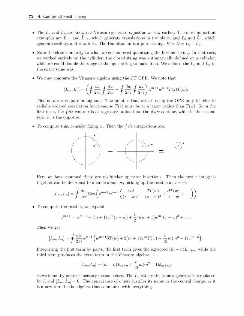
72 4. Conformal Field Theory
• The Ln and Ln are known as Virasoro generators, just as we saw earlier. The most important
examples are L−1 and L−1, which generate translations in the plane, and L0 and L0, which
generate scalings and rotations. The Hamiltonian is a pure scaling, H = D = L0 + L0.
• Note the close similarity to what we encountered quantizing the bosonic string. In that case,
we worked entirely on the cylinder: the closed string was automatically defined on a cylinder,
while we could double the range of the open string to make it so. We defined the Ln and Ln in
the exact same way.
• We may compute the Virasoro algebra using the TT OPE. We note that
[Lm, Ln] =
(∮dz
2πi
∮dw
2πi−∮
dw
2πi
∮dz
2πi
)zm+1wn+1T (z)T (w).
This notation is quite ambiguous. The point is that we are using the OPE only to refer to
radially ordered correlation functions, so T (z) must be at a larger radius than T (w). So in the
first term, the∮dz contour is at a greater radius than the
∮dw contour, while in the second
term it is the opposite.
• To compute this, consider fixing w. Then the∮dz integrations are:
Here we have assumed there are no further operator insertions. Then the two z integrals
together can be deformed to a circle about w, picking up the residue at z = w,
[Lm, Ln] =
∮dw
2πiRes
(zm+1wn+1
(c/2
(z − w)4+
2T (w)
(z − w)2+∂T (w)
z − w+ . . .
)).
• To compute the residue, we expand
zm+1 = wm+1 + (m+ 1)wm(z − w) +1
2m(m+ 1)wm1(z − w)2 + . . . .
Then we get
[Lm, Ln] =
∮dw
2πiwn+1
(wm+1∂T (w) + 2(m+ 1)wmT (w) +
c
12m(m2 − 1)wm−2
).
Integrating the first term by parts, the first term gives the expected (m− n)Lm+n, while the
third term produces the extra term in the Virasoro algebra,
[Lm, Ln] = (m− n)Lm+n +c
12m(m2 − 1)δm+n,0
as we found by more elementary means before. The Ln satisfy the same algebra with c replaced
by c, and [Lm, Ln] = 0. The appearance of c here justifies its name as the central charge, as it
is a new term in the algebra that commutes with everything.

73 4. Conformal Field Theory
• To understand the appearance of the central charge, note that the diffeomorphisms δz = zn+1
give the Witt algebra, as we saw earlier. The extra term for conformal transformations arises
because of the extra Weyl rescaling. (is this right? how does c affect the Weyl rescaling?)
Using the Virasoro algebra, we can generate states.
• Suppose we have a state |ψ〉 which is an eigenstate of L0 and L0,
L0|ψ〉 = h|ψ〉, L0|ψ〉 = h|ψ〉.
On the cylinder, this correspond to a state of energy
E
2π= h+ h− c+ c
24.
Hence we refer to h and h as the energy of the state. Furthermore, the angular momentum of
the state is h− h. Note the tempting similarity with the conformal weight; we will make this
more precise with the state-operator correspondence.
• By acting with Ln operators, we get further states with eigenvalues
L0Ln|ψ〉 = (LnL0 − nLn)|ψ〉 = (h− n)Ln|ψ〉
so Ln lowers the energy h by n, while Ln lowers the energy h by n.
• If the spectrum is bounded below, there must be states annihilated by Ln and Ln for all n > 0.
These are called primary states; they are the states of lowest energy. By acting with the L−nand L−n, we can construct an infinite tower of higher-energy states, called the descendants. The
primary state condition corresponds to the physical state condition in covariant quantization.
• In the language of representation theory, a primary state is a highest weight state, and the whole
resulting set of states generated from a primary is called a Verma module (formal definition?)
; it is a representation of the Virasoro algebra.
• One might wonder how these representations decompose into Lorentz representations, as the
Lorentz algebra is a subalgebra of the Virasoro algebra in any dimension. Generically there
may be massive representations, but the masses must form a gapless, continuous spectrum.
• The vacuum state |0〉 has zero energy, h = h = 0, and is hence annihilated by Ln and Ln for
all n ≥ 0. This accords with our intuition that the vacuum states should have the greatest
symmetry. However, it is impossible for all of the Ln and Ln to annihilate the vacuum, as this
would leave no room for the central charge term.
• It is possible that the states in the Verma module are dependent. A linear combination of
states that vanishes identically is called a null state. The existence of null states depends on
the values of h and c.
• It is also physically important to impose unitarity. However, it isn’t possible to talk about this
in Euclidean signature, so we must return to the Euclidean cylinder, and from there to the
Minkowski cylinder, where the Hamiltonian density is
H = Tww + Tww =∑n
Lne−inσ+
+ Lne−inσ− .
74 4. Conformal Field Theory
For the Hamiltonian to be Hermitian, we require
Ln = L†−n
just as we saw when quantizing the string.
• Furthermore, we must demand the Hilbert space does not contain negative norm states. We
cannot simply dismiss these states as unphysical; we could only do this for the string because
the conformal symmetry there was gauged. (right?) This leads to some tight constraints.
• First, note that for any primary state |ψ〉,
|L−1|ψ〉|2 = 〈ψ|L1L−1|ψ〉 = 〈ψ|[L1, L−1]|ψ〉 = 2h〈ψ|ψ〉
which must be nonnegative, so h ≥ 0. The only state with h = 0 is the vacuum state |0〉.
• Now consider the norm
|L−n|0〉|2 = 〈0|[Ln, L−n]|0〉 =c
12n(n2 − 1).
For this to be nonnegative, we require c ≥ 0. When c = 0, the only state in the vacuum
module is the vacuum itself; in fact, it turns out this is the only state in the entire theory.
Any nontrivial CFT has c > 0. There are many more such requirements; the constraints are
sufficient to classify and solve all CFTs with c < 1.
4.6 The State-Operator Correspondence
The states in a CFT can be related to operators by the state-operator correspondence.
• States and local operators are on a very different footing in quantum field theory. Local
operators live at a point, while states are wavefunctionals over field configurations defined over
an entire spatial slice. However, in a CFT the distant past in the cylinder is mapped to a single
point z = 0, giving rise to a correspondence between them.
• To make this more precise, note that in Euclidean QFT, a state Ψi[φi(σ)] at time τi evolves to
Ψf [φf (σ), τf ] =
∫Dφi
∫ φ(τf )=φf
φ(τi)=φi
Dφ e−S[φ]Ψi[φi(σ), τi].
For a CFT on the plane, we simply replace timeslices with surfaces of constant r,
Ψf [φf (σ), rf ] =
∫Dφi
∫ φ(rf )=φf
φ(ri)=φi
Dφ e−S[φ]Ψi[φi(σ), ri].
• Now suppose we take the initial state to the infinite past, z = 0. Then we must integrate over
the whole disc |z| < rf , and the initial state wavefunctional which weights the path integral just
translates to a weighting factor at z = 0, which can be expressed as a local operator. Hence
the effect of the initial state can be equivalently written as an operator insertion,
Ψ[φf , r] =
∫ φ(r)=φf
Dφ e−S[φ]O(z = 0).
This gives a correspondence between local operators and states in the infinite past. We take
a Heisenberg-like picture where we imagine states as extending through time, or in this case
through radii. Hence the state Ψ[φf , r] is just a snapshot of the state |O〉 at a given moment.
75 4. Conformal Field Theory
• The state-operator correspondence works because we can map the infinite past goes to a single
point. Similarly, CFTs on RD can be conformally mapped to R× SD−1. (how to show this
explicitly?)
• The state-operator correspondence shouldn’t be confused with the construction of the Hilbert
space by creation operators in ordinary QFT, as these operators are not local. Furthermore, in
ordinary QFT, we can always map a set of operators to a state, e.g. by having them all act on
the vacuum at the same time. It is only in CFT that the map goes the other direction, since in
CFT we can shrink a “timeslice” to a point.
• The Euclidean path integral projects out the vacuum state when integrated over infinite Eu-
clidean time. As such, the vacuum state |0〉 corresponds to the identity operator and is hence
sometimes written as |1〉.
We now consider some simple consequences of this result.
• First, note that for a primary operator O and corresponding state |O〉,
Ln|O〉 =
∮dz
2πizn+1T (z)O(z = 0)
where the right-hand side is understood to be underneath a path integral. Applying the OPE,
Ln|O〉 ∼∮
dz
2πizn+1
(hOz2
+∂Oz
).
• As a result, we find that
L−1|O〉 = |∂O〉
which in fact holds for all operators; it simply states that L−1 is a translation. We also have
L0|O〉 = h|O〉
which holds for any operators with well-defined transformations under scaling, and
Ln|O〉 = 0, n > 0
which tells us that primary operators correspond to primary states.
• Hence computing the spectrum of weights of primary operators corresponds to computing the
spectrum of energies and angular momenta of primary states. Going the other way, diagonalizing
D and L on the set of states will give us a set of local operators with good transformation
properties, which we merely postulated existed earlier.
• The state-operator correspondence also explains why the OPE works so well in CFT. Consider
a correlation function with two local operators inserted nearby. As argued earlier, we can
perform the path integral over a small disk containing them, yielding a weighting function for
the remaining path integral, which behaves like a state specified on the boundary of the disk.
Putting the origin at the center of this disk, the state may be viewed as the time evolution of
a state specified in the infinite past, which then corresponds to a local operator, precisely the
right-hand side of the OPE. This furthermore tells us the OPE is an exact statement as long
as the operators are closer to each other than to any other operators.
76 4. Conformal Field Theory
We now apply the operator-state correspondence to the free scalar field.
• It’s convenient to expand X in a Fourier series on the Euclidean cylinder,
X(w,w) = x+ α′pτ + i
√α′
2
∑n6=0
1
n(αne
inw + αne−inw)
following our treatment of the closed string. The constraint of reality of X in Minkowski space
gives us α†n = α−n and α†n = α−n.
• As we’ve seen, X is not primary, so we instead work with ∂X,
∂wX(w) = −√α′
2
∑n
αneinw, α0 = i
√α′
2p.
Note that we have restricted to the holomorphic component. Next, since ∂X is a primary field
of weight (1, 0) we can easily transform to the plane,
∂zX(z) =
(∂z
∂w
)−1
∂wX(w) = −i√α′
2
∑n
αnzn+1
.
• We can invert this expression with a contour integral,
αn = i
√2
α′
∮dz
2πizn∂X(z).
The commutation relations can be found using the OPE,
[αm, αn] = − 2
α′
(∮dz
2πi
∮dw
2πi−∮
dw
2πi
∮dz
2πi
)zmwn∂X(z)∂X(w)
which by the same trick as before, gives
[αm, αn] = − 2
α′
∮dw
2πiResz=w
(zmwn
(−α′/2
(z − w)2+ . . .
))= m
∮dw
2πiwm+n−1 = mδm+n
where we Taylor expanded zm = wm +mwm−1(z − w) + . . .. The final result is just what we
found for the bosonic string.
• Now, we know that the Fock space is defined by acting with creation operators α−m with m > 0
on the vacuum |0〉, so a general state is given by∏m>0
αkm−m|0, p〉
where the value of p corresponds to the zero mode α0. We would like to explicitly construct
the operator-state correspondence.
• Suppressing the zero mode, we start with the vacuum state |0〉, and would like to show explicitly
that it corresponds with the identity operator. The defining property of the vacuum state is
αm|0〉 = 0 for m > 0, while the ground state wavefunctional is
Ψ0[Xf ] =
∫ Xf (τ)
DX e−S[X].
77 4. Conformal Field Theory
Upon acting with αm, we get
αmΨ0[Xf ] ∝∫ Xf
DX e−S[X]
∮dw
2πiwm∂X(w).
Note that αn is not a local operator; instead it corresponds to insertions over an entire timeslice
of constant radius. We must evaluate the right-hand side at a larger radius, since the state only
vanishes after acting with αn.
• Since the path integral favors smooth functions, we simply assume X is smooth. But then the
contour integral vanishes for m ≥ 0, giving the desired result.
• Next, we claim that
α−m|0〉 = |∂mX〉 =
∫DX e−S[X]∂mX(z = 0).
In order to check this, we act with αn,
αn|∂mX〉 ∼∫ Xf (τ)
DX e−S[X]
∮dw
2πiwn∂X(w)∂mX(z = 0).
We then use the OPE on the right-hand side, which gives∮dw
2πiwn∂m−1
z
1
(w − z)2
∣∣∣∣z=0
= m!
∮dw
2πiwn−m−1 ∝ δm,n
just as expected.
• Finally, the zero mode arises by insertion of the primary operator eipX ,
|0, p〉 ∼∫DX e−S[X]eipX(z=0).
More generally, a complete set of local operators is given by products of eipX with terms like
∂nX and ∂nX.
Finally, we briefly comment on the open string.
• The open string lives on the infinite strip with spatial coordinate σ ∈ [0, π]. Upon the same
conformal mapping z = e−iw, it is mapped to the upper-half plane Im z ≥ 0, with the endpoints
of the string mapped to the real axis.
• We have lost translational invariance in the imaginary direction, but preserve it in the real
direction, so Tαβtβ remains a conserved current, where tα is tangent to the real axis. Letting
nα be the normal vector, Neumann boundary conditions mean that none of the current flows
out of the boundary, so
Tαβnαtβ = 0
at Im z = 0.
78 4. Conformal Field Theory
• In complex coordinates, Tzz = Tzz at Im z = 0. This allows us to extend Tzz to the whole
complex plane by defining
Tzz(z) = Tzz(z).
Hence we may equivalently think of the stress tensor as defined on the whole plane, but only
containing the holomorphic component T . This allows us to carry over all our previous results,
with only one set of Virasoro generators.
• A similar trick can be used to compute the propagator for the free scalar field. The scalar
field X(z, z) is only defined for the upper-half plane and obeys Neumann boundary conditions.
These can be accounted for by adding image charges,
G(z, z, w,w) = −α′
2log |z − w|2 − α′
2log |z − w|2.
In particular, if z and w lie on the real axis, then the propagator is the same as the closed
string, but multiplied by a factor of 2.
• The infinite past is still represented by z = 0, a point on the boundary. More generally, this
means the state-operator map only works for local operators defined on the boundary. This
ensures that theories on a strip have fewer states than those on the cylinder. For example,
Neumann boundary conditions require ∂X = ∂X on the boundary, so on the strip they can
only give rise to the same state. This reflects the halving of oscillator modes for the open string
we saw earlier.
79 5. String Interactions
5 String Interactions
5.1 Motivation
Now we turn to a heuristic discussion of string interactions.
• As motivated earlier, one can describe string interactions by evaluating a series of “string
diagrams”, where the worldsheet has nontrivial topology, and Weyl invariance on the worldsheet
can be used to simplify the diagrams. For tree-level scattering of n closed strings, it can be
shown that the worldsheet can be converted to a sphere with n punctures.
• At each puncture, there must appear some local operator in the worldsheet QFT with the
quantum numbers of the external string state |Λ〉 mapped to that point, called the vertex
operator VΛ. This “state–operator correspondence” is a common idea in conformal field theories.
• Heuristically, for each particle type there should be a local operator WΛ(σ, τ). It must be a
scalar under reparametrizations of σ and τ , and have the same Lorentz quantum numbers as
Λ. We can try to build WΛ out of Xµ and its derivatives.
• Since the tachyon is a Lorentz scalar, we can simply take W = 1, while for the graviton the
simplest spin two operator is Wµν = ∂αXµ∂αXν .
• However, we must also take into account spacetime translations. Under the global symmetry
Xµ → Xµ + aµ, the wavefunction of an external state of momentum kµ is multiplied by eik·a.
This can be accounted for by taking a factor of eik·X in the vertex operator. Finally, the vertex
operator should be integrated over the worldsheet, since it may appear anywhere on it, giving
VΛ(k) =
∫d2σ√hWΛ(σ, τ)eik·X .
This handles both emission and absorption; by convention k is always directed inward.
• Finally, to compute scattering amplitudes, we would expect a path integral to give
A(Λ1, k1, . . . ,ΛM , kM ) = κM−2
∫DXDh e−S
M∏i=1
VΛi(ki)
where S is the Polyakov action and κ is a coupling constant. Actually deriving this require
background in string field theory and is far beyond our scope.
• In this section, we will focus on evaluating the tree-level contribution, which for closed strings
gives a sphere; accounting for higher-order contributions involves a sum over Riemann surfaces
of arbitrary genus.
• Focusing on the tree-level contribution, it is most convenient to stereographically project the
sphere to the plane. Since we have fixed the metric h, the path integral simplifies to
A = κM−2
∫DX(x, y) exp
(− 1
2π
∫d2x ∂αXµ∂
αXµ
) M∏i=1
VΛi(ki) ≡ κM−2
⟨M∏i=1
VΛi(ki)
⟩
which is simply a free field theory correlator that can be directly evaluated.
80 5. String Interactions
• However, there are further issues involving the path integral measure. As usual, we should mod
out by gauge symmetries, but our final configuration has residual diffeomorphism symmetry.
This is easiest to see by adopting complex coordinates in the plane. The worldsheet metric must
be in the form ds2 = eφdzdz, and changing coordinates to w(z) where w is analytic preserves
this. Infinitesimally, we have transformations δz = ε(z) where ε is holomorphic.
• However, we must ensure that δz = ε(z) does not have a pole at the point at infinity, which
corresponds to a point in the original sphere. Equivalently, if z = 1/z, then δz cannot have a
pole at zero, but
δz = −ε(z)z2
which implies ε(z) is a quadratic polynomial, δz = a + bz + cz2. These generate a group
isomorphic to SL(2,C).
• As an explicit example, consider the scattering of M tachyons. Then
A = κM−2
∫ M∏i=1
d2zi
⟨M∏i=1
eiki·X(zi)
⟩.
The free field correlator can be evaluated by completing the square, where ki plays a role like a
source in ordinary field theory, giving
A = κM−2
∫ M∏i=1
d2zi∏i<j
exp
(1
2(ki · kj)G(zi, zj)
)where G is the propagator of the free field Xµ, satisfying
∆zG(z, z′) = 2πδ2(z − z′).
• Taking the inverse Fourier transform, we find
G(z, z′) = −2π
∫d2q
4π2
eiq·(z−z′)
q2= log(µ|z − z′|)
where µ is an arbitrary constant which regulates the IR divergence. (prove this) Therefore
we have
A = κM−2
∫ M∏i=1
d2zi∏i<j
|zi − zj |ki·kj/2.
• This integral diverges because we have not accounted for the SL(2,C) gauge symmetry. This
gauge symmetry is conventionally fixed by setting
z1 = 0, z2 = 1, z3 =∞.
The terms involving z3 then multiply to |z3|−k23/2 = |z3|m
2/2 by momentum conservation, giving
a constant which can be ignored. We hence have
A = κM−2
∫ M∏`=4
d2z`
M∏j=4
|zj |k1·kj/2|1− zj |k2·kj/2∏
4≤i<j≤M|zi − zj |ki·kj/2.
In particular, for the four-point function we have
A = κ2
∫d2z4 |z4|k1·k4/2|1− z4|k2·k4/2.
81 5. String Interactions
• To derive these results more properly, we must ensure the gauge symmetries are not anomalous.
One manifestation of SL(2,C) gauge symmetry is that V is SL(2,C) invariant. However, since
V =
∫d2z eik·X(z)
it appears that eik·X must be an operator of dimension two. Since Xµ is dimensionless, eik·X
would classically have dimension zero, but it can receive an anomalous dimension. These can
appear even for free field theories, as long as we work in 1 + 1 dimensions. (really?)
• Concretely, for an operator Y of dimension p, we have
〈Y (z)Y (0)〉 ∝ |z|−2p.
From our computations above, we already know that
〈eik·X(z)e−ik·X(0)〉 = |z|−k2/2
which indicates that the dimension is k2/4. Since this must be equal to two, we have k2 = 8,
which gives the correct tachyon mass for the critical string. A similar computation for graviton
scattering shows that the gravitons must be massless for consistency.
Next, we apply the same ideas to open strings.
• A tree-level open string diagram can be mapped onto a disc or a half-plane, with the vertex
operators on the boundary. Therefore, the vertex operators take the form
V =
∫dτ√hττ U(τ), U = Weik·X
where τ is a parameter on the boundary of the worldsheet; invariance of V under conformal
rescalings now require that U should have dimension one.
• For a spin zero particle we may take W = 1. Then it turns out that V has dimension k2/2,
and since the integral is only over the boundary, V must have dimension one. Then k2 = 2,
corresponding to the open string tachyon. For spin one, we may try W = dXµ/dτ , which
requires k2 = 0.
• Mapping the worldsheet to the upper half-plane, the amplitude is
A(k1, . . . , kM ) = gM−2
∫dx1 . . . dxM
⟨M∏i=1
eiki·X(xi)
⟩
where g is the open string coupling constant. The residual gauge symmetries are conformal
maps from the plane to itself, which preserve the real axis and are nonsingular at infinity; these
take the form δz = a+bz+cz2 where a, b, and c are real, and correspond to the group SL(2,R).
• Note that conformal transformations can only produce cyclic permutations of the xi, so a given
string diagram fixes their cyclic order.
82 5. String Interactions
• Furthermore, it turns out that the endpoints of open strings may carry gauge charges. This may
be motivated from the original purpose of string theory as a model for the strong interactions,
where the string corresponds to a flux tube and quarks and antiquarks sit at the endpoints. (In
fact, the first attempt to include fermions to describe baryons eventually led to the development
of superstring theory.)
• One concrete realization of this is to consider a set of N space-filling D-branes. Then each
endpoint of the open string can lie on any of the D-branes, so the state of the two endpoints is
described by an N ×N matrix.
• For gauge group U(n), if we let the endpoints of the string transform in the fundamental and
antifundamental, each vertex operator comes with a matrix λij transforming in the adjoint. If
the vertex operators come in the order 12 . . .M , we pick up a group theory factor of tr(λ1 . . . λM )
as each antiquark is contracted with the next quark. This is called a Chan-Paton factor.
• We use the SL(2,R) symmetry to fix
x1 = 0, xM−1 = 1, xM =∞
so that the remaining xi lie in (0, 1). We will also need the Green’s function G(z, z′) which
satisfies the Neumann boundary conditions
∂G(x+ iy, z′)
∂y
∣∣∣∣y=0
= 0.
This may be found by the method of images, which gives
G(z, z′) = log |z − z′|+ log |z − z′|.
However, we are actually interested in the case where z and z′ are both on the real axis, in
which case G(x, x′) = 2 log |x− x′|, differing from G only by a factor of 2. This also accounts
for the factor of 2 in the dimension of V above.
• Plugging everything in, for tachyon scattering we have the result
A = gM−2
∫0<x2<...<xM−2<1
dx2 . . . dxM−2
M−2∏j=2
|xj |k1·kj |1−xj |kj ·kM−1∏
2≤`<m≤M−2
|x`−xm|k`·km .
This is the Koba–Nielsen M -particle generalization of the Veneziano amplitude. For M = 4 it
simplifies to
A = g2
∫ 1
0dxxk1·k2(1− x)k2·k3 = g2B
(−s
2− 2,− t
2− 2
)which is the Veneziano amplitude.
• It is also possible to have diagrams with both external open and closed strings. These can be
evaluated by mapping the worldsheet to the upper half-plane, where the open string vertex
operators are on the boundary and the closed string vertex operators in the bulk.
83 5. String Interactions
5.2 Vertex Operators
Next, we turn to a more detailed study of vertex operators, focusing on open strings.
• Consider a local operator at the string endpoint, A(τ) ≡ A(0, τ). Since the string Hamiltonian
is L0 − a, we have
A(τ) = eiτL0A(0)e−iτL0 .
• We say A(τ) is a boundary primary operator with conformal dimension J if, under a change of
variable τ → τ ′, we have
A′(τ ′) =
(dτ
dτ ′
)JA(τ).
This is equivalent to our definition of the conformal dimension in the previous section. (show
this) Such operators transform “nicely” and are rather special; not every operator can be
expanded as a linear combination of primary operators.
• The above condition is easier to handle at the infinitesimal level. For δτ = ε(τ), we have
δA(τ) = −εdAdτ− JA dε
dτ
by the definition above. The Lm generate transformations with ε = ieimτ , so equivalently
[Lm, A(τ)] = eimτ(−i ddτ
+mJ
)A(τ).
• If A(τ) has an expansion in Fourier modes
A(τ) =∑m
Ame−imτ
then this condition is equivalent to
[Lm, An] = (m(J − 1)− n)Am+n.
• It is straightforward to show that Xµ(τ) has J = 0, as
Xµ(τ) = xµ + pµτ + i∑n6=0
αµnne−inτ
and
[Lm, Xµ(τ)] = iαm − i
∑n 6=0
αµm+ne−inτ = −i
∑n
αµne−i(n−m)τ = −ieimτ d
dτXµ(τ).
Furthermore, the momentum operator Xµ(τ) has J = 1. However, Xµ(τ) is not a boundary
primary operator at all. It’s easiest to show these using the expansion in Fourier modes.
• We have seen earlier that vertex operators should be primaries of dimension 1. Another way to
see this makes sense is that if A(τ) has dimension 1 and |φ〉 is a physical state, then [Lm, A0] = 0,
and hence A0|φ〉 is also a physical state. This is what we expect, as an emission or absorption
should map a physical state to another.
84 5. String Interactions
Now we consider some examples of vertex operators.
• By the same arguments as before, we expect vertex operators to contain a factor of eik·x(τ),
where x(τ) is the string’s center of mass position,
xµ(τ) = xµ + pµτ.
However, this is not a local operator, so we instead consider eik·X(τ). This exponential requires
normal ordering, giving
V (k, τ) = :eik·X(0,τ) : = exp
(k ·
∞∑n=1
α−nneinτ
)eik·x(τ) exp
(−k ·
∞∑n=1
αnne−inτ
).
This differs from the unordered expression by the divergent sum α′k2∑
1/n, by the BCH
formula. As motivated earlier, this is the vertex operator for a tachyon.
• Naively, products of primary operators would be primary operators whose dimension is the
sum of the product factors’. Indeed, this appears to be true if we naively use commutator
identities above. The problem is that some products may be undefined without a subtraction
or regularization scheme. In this case, we can remove the singularities by normal ordering, but
typical normal-ordered products such as :Xµ(τ)Xµ(τ) : aren’t primaries at all.
• To compute the dimension of V (k, τ), we note that
[αµp , ek·α−n ] = pδp,nk
µek·α−n
which easily leads to
[Lm, ek·α−n ] =
1
2nk · αm−n, ek·α−n
where the right-hand side contains an anticommutator, by using the commutator product rule
to split apart Lm, and then using our previous identity.
• Now we need to evaluate [Lm, V (k, τ)]. By expanding in a Taylor series, we have
[Lm, eik·X(0,τ)] = −ieimτ d
dτeik·X(0,τ)
which indicates that eik·X(0,τ) has dimension zero, as we’d expect. When we add normal ordering,
the right-hand side remains normal ordered, but the left-hand side is not. This causes the two
sides to differ, introducing an extra term that yields the conformal dimension.
• Hence we can focus on the terms in [Lm, V (k, τ)] that are not normal ordered. This computation
can be done by using the commutator product rule to split apart Lm, then using our previous
identity. This produces m terms with creation operators on the far left, precisely
1
2
m∑n=1
k · αm−neinτV (k, τ) =
[1
2
m∑n=1
k · αm−neinτ , V (k, τ)
]+ :
1
2
m∑n=1
k · αm−neinτV (k, τ) : .
The second term contributes to :(d/dτ)eik·X(0,τ) : as in the non-normal ordered case, while the
extra commutator term is[1
2
m∑n=1
k · αm−neinτ , V (k, τ)
]=
1
2
m∑n=1
k2eimτV (k, τ) =1
2mk2eimτV (k, τ)
which yields a conformal dimension J = k2/2, in accordance with our earlier computation.
85 5. String Interactions
• This is indeed a vertex operator when k2 = 2, which is precisely the on-shell condition for the
tachyon. Hence V (k, τ) is the vertex operator for the open string tachyon.
• Next, we can consider vertex operators for the photons at level one. One candidate which could
have the right dimension is
Vζ(k, τ) = ζ · dXdτ
exp(ik ·X), k2 = 0.
This expression is already normal ordered, provided that ζ · k = 0, as eik·X is already normal
ordered for k2 = 0, and commuting components of ζ ·dX/dτ through it gives terms proportional
to ζ · k. Hence this operator is a primary of dimension 1. It is the vertex operator for a photon
of polarization ζ.
• We may also define vertex operators for states of zero norm. For instance,
V (k, τ) = −i ddτ
exp(ik ·X), k2 = 0
is a vertex operator for the zero norm longitudinal photon state. The fact that this state is not
physical is reflected in the fact that V (k, τ) is a τ derivative, so V0 vanishes.
• Finally, we can consider vertex operators at level two. Candidates with the right dimension are
ζµνXµXν : exp(ik ·X) : , k2 = −1
which is free of short-distance singularities if
kµζµν = ηµνζ
µν = 0.
This gives a total of D(D − 1)/2 − 1 degrees of freedom, which is just enough to account for
the symmetric traceless tensor of SO(D − 1) that appears at level two.
5.3 Bosonic Open Strings
Now we consider scattering amplitudes for open strings.
• Instead of using the path integral to evaluate a tree-level scattering amplitude, we will use a
setup like that of worldline QFT, which we saw in the notes on Quantum Field Theory. Each
diagram is a graph, and each edge of the graph corresponds to a worldline, which yields a
propagator factor. One also writes down a factor for each vertex.
• We will take a slightly different route. Note that if we start with any tree-level open string
diagram, with M external particles, we can deform it to the form of a single line on which
M − 2 external string emissions are attached. This leads to the ansatz
A = gM−2〈φ1|V2(k2)∆V3(k3) . . .∆VM−1(kM−1)|φM 〉
where ∆ is the string propagator and the Vi are vertex operators. This manifestly contains
poles due to on-shell propagators, as required by tree-level unitarity. However, symmetry under
cyclic permutations of the external particles (i.e. duality) is not manifest.
86 5. String Interactions
• For scalar field theory, where (∂2 +m2)φ = 0, the propagator is simply (∂2 +m2)−1. For free
open strings, the closest analogue of the first equation is (L0 − 1)|φ〉 = 0, so we define the
propagator to be
∆ = (L0 − 1)−1 =
∫ 1
0zL0−2 dz.
• For the vertex operators, it will be useful to define z = eiτ , so that
[Lm, V (k, z))] =
(zm+1 d
dz+mzm
)V (k, z), Xµ(z) = xµ − ipµ log z + i
∑n6=0
1
nαµnz
−n.
• It is also useful to write the tachyon vertex operator as
V0(k, z) ≡ :eik·X(z) : = Z0W0
where Z0 is the zero mode operator,
Z0 = eik·x+k·p log z = eik·xzk·p+1 = zk·p−1eik·x
and W0 is the remaining factor,
W0 = exp
(k ·
∞∑n=1
αnnzn
)exp
(−k ·
∞∑n=1
αnnz−n
).
• Similarly, the vertex operator for a massless photon is
V (ζ, k, z) = ζ · X(z)eik·X(z)
where a dot indicates a derivative with respect to τ = −i log z.
• Next, we need to account for the external states. These can be constructed by a similar trick to
that of quantum field theory. In quantum field theory, if we start with an arbitrary state with
at least some overlap with the vacuum, then after evolution in imaginary time it will evolve to
the vacuum state because everything else exponentially decays away. Similarly, to get, e.g. the
lowest-energy state with a given conserved charge, we can start with an arbitrary state with
the same charge and do the same.
• In string theory, the operators which give the desired states are precisely the vertex operators.
That is, we have
|Λ, k〉 = limτ→i∞
e−iτVΛ(k, τ)|0, 0〉, 〈Λ, k| = limτ→−i∞
eiτ 〈0, 0|VΛ(k, τ).
Note that we do not have to actually Wick rotate to do this; the operator VΛ(k, τ) with τ
imaginary is defined in exactly the same way as VΛ(k, τ) with τ real. This result is called the
operator–state correspondence, and is an important principle in conformal field theory.
• Note that we are using the state |0, 0〉. It is formally the vacuum of the 2D worldsheet QFT.
However, it is not interpreted as a physical state; it is a tachyon with the momentum off-shell.
87 5. String Interactions
• We can check this explicitly for the tachyon vertex operator. By design, acting with W0 on
|0, 0〉 will do nothing in the limit τ → i∞, leaving
Z0|0, 0〉 = eik·xzk·p+1|0, 0〉 = z|0, k〉
since eik·x translates by k in momentum space. The factor of e−iτ precisely cancels the extra z.
• Finally, the propagator can also be expressed as
∆ =
∫ ∞0
dτ e−τ(L0−1)
where the integrand generates evolution in imaginary time τ . The full amplitude is hence written
in terms of infinite imaginary time evolution, with vertex operators V1 and VM inserted at infinity
and the other Vi inserted at finite imaginary times; we integrate over these intermediate times.
• One can show that ghosts decouple as required, preserving tree-level unitarity. Another impor-
tant formal task is to show that the amplitude has cyclic symmetry. Substituting in our results
above and using the fact that (L0 − 1)|φ1〉 = (L0 − 1)|φM 〉 = 0, the amplitude becomes
A = gM−2
∫ 1
0
dz3 . . . dzM−1
z3 . . . zM−1〈φ1|V (k2, 1)V (k3, z3) . . . V (kM−1, z3 . . . zM−1)|φM 〉.
The ordering can be made more explicit by changing variables to yi = z3z4 . . . zi, giving
A = gM−2
∫ 1
0
(M−1∏i=3
θ(yi−1 − yi)dyiyi
)〈φ1|V (k2, y2) . . . V (kM−1, yM−1)|φM 〉.
Now, applying the operator-state correspondence, the expectation value becomes
limy1→∞
limyM→0
y1
yM〈0, 0|V (k1, y1) . . . V (kM , yM )|0, 0〉.
• We must now evaluate an expectation value in the “unphysical” vacuum state |0, 0〉. Now,
string theory can be thought of as a two-dimensional field theory with an enormous symmetry
group, and SL(2,R) generated by L−1, L0, L1 is the non-anomalous part of the Virasoro algebra.
The vacuum is indeed SL(2,R) invariant, L1|0, 0〉 = L0|0, 0〉 = L1|0, 0〉 = 0. This is, of course,
the same residual SL(2,R) symmetry we encountered earlier.
• Infinitesimally, these SL(2,R) transformations generate the change
y → y′ = y + λ−1 + λ0y + λ1y2.
One might wonder why the 2× 2 matrices in SL(2,R) have a natural nonlinear action on the
line; it turns out y transforms like v1/v2 for a vector (v1, v2)T . The general transformation is
y → y′ =ay + b
cy + d
conventionally scaled so that ad− bc = 1. This is called a Mobius transformation.
88 5. String Interactions
• Mobius transformations give us the freedom to move the points at y1 and yM . As for the path
integral, we must quotient out by the volume of SL(2,R) to avoid overcounting. After some
calculation, we find that the measure for the integral is
dµM (y) = δ(yA − y0A)δ(yB − y0
B)δ(yC − y0C)(yA − yB)(yA − yC)(yB − yC)
M∏i=2
θ(yi−1 − yi)M∏j=1
dyj
where we have fixed three of the yi’s, namely yA, yB, and yC , to specific values. This establishes
cyclic symmetry in the integration variables yi. Finally, cyclic symmetry in the product of
vertex operators can also be shown, though we omit this calculation.
With all of this setup, we are now finally ready for some examples.
Example. The three-tachyon amplitude. This is
A = g〈0,−k1|V0(k2, τ)|0, k3〉
where all momenta are directed inward and τ is an arbitrary constant which we do not need to
integrate over, following the arguments above. To verify the value of τ does not matter, note that
A = g〈0,−k1|eiτL0V0(k2, 0)e−iτL0 |0, k3〉 = g〈0,−k1|V0(k2, 0)|0, k3〉
where we used the physical state condition (L0 − 1)|0, k〉 = 0. Plugging in the form of the tachyon
vertex operator, the oscillator part W0 does nothing, since there are no excitations to annihilate, so
A = g〈0,−k1|Z0|0, k3〉 = g〈0,−k1|eik2·x|0, k3〉 = g〈0,−k1|0, k2 + k3〉 = gδ(k1 + k2 + k3).
The momentum-conserving delta function is generic and we will omit it below.
Example. The tachyon-tachyon-photon amplitude, where the photon has polarization ζ. Then
g〈0,−k1|V (ζ, k2)|0, k3〉 = g〈0,−k1|ζ · X(1)V0(k2, 0)|0, k3〉
where we simply set τ = 0 in the vertex operator, following the discussion above. (finish)
89 6. String Compactification
6 String Compactification
6.1 Kaluza–Klein Theory
Compactifying the extra dimensions of string theory is one way to get a realistic result. In this
section, we consider the simple example of one compact dimension and a closed bosonic string.
• We take the compact dimension to be
X25 ∼ X25 + 2πR
so the background spacetime is R1,24 × S1. This is a Kaluza–Klein compactification.
• We know that the closed string’s massless fields are a traceless symmetric tensor, an antisym-
metric tensor, and the dilaton. Following the original setup of Kaluza–Klein theory, we consider
what happens to the symmetric tensor.
• In Einstein frame, the metric in D = 26 is decomposed into a D = 25 metric Gµν , a vector Aµ,
and a scalar σ,
ds2 = GµνdXµdXν + e2σ(dX25 +AµdX
µ)2.
Here, Greek indices run over the noncompact dimensions 0, 1, . . . , 24 only.
• Diffeomorphisms affecting the noncompact dimensions lead to the expected diffeomorphism
symmetry of Gµν as a 25-dimensional metric, while diffeomorphisms affecting the compact
direction, δX25 = Λ(Xµ) correspond to δAµ = ∂µΛ. This indicates that Aµ is a 25-dimensional
gauge field.
• One can show that the D = 26 Ricci scalar R(26) is
R(26) = R− 2e−σ∇2eσ − 1
4e2σFµνF
µν
where R is the D = 25 Ricci scalar. Therefore, the Einstein–Hilbert action is
S =1
2κ2
∫d26X
√−G(26)R(26) =
2πR
2κ2
∫d25X
√−G eσ
(R− 1
4e2σFµνF
µν + ∂µσ∂µσ
)where we have neglected any dependence on the compact dimension, since we only are interested
in the low-energy effective action. This gives the interactions between the D = 25 fields.
• The D = 25 action is not quite of the Einstein–Hilbert form, because of the eσ coefficient, but
we may remove it by another change of frame. After this change, we see there is no potential
dictating the vev of σ, which determines the physical size of the compactified dimension. In
this particular case, a potential does arise as a one-loop effect.
• Such “moduli fields” are ubiquitous in compactifications of string theory and often lead to
unwanted massless scalars, especially in supersymmetric theories. One must add a mechanism
which gives them a potential and dynamically fixes the vev.
• We can also consider the Kaluza–Klein reduction of the other fields. The dilaton Φ simply
remains a scalar, while the Kalb–Ramond field reduces to a 2-form Bµν and a vector field
Aµ = Bµ 25. Note that in four dimensions, Kalb–Ramond fields have one degree of freedom; the
corresponding particle is a massless scalar that behaves like an axion. Hence the low-energy
physics consists of a metric, two U(1) gauge fields, and three massless scalars.
90 6. String Compactification
More generally, we can consider what happens when the fields depend on the compact dimension.
• For simplicity, consider the scalar field Φ. Since it must be periodic in X25, it may be expanded
in a Fourier series,
Φ(Xµ, X25) =∑n
Φn(Xµ)einX25/R.
Since it is a real scalar, Φ∗n = Φ−n.
• Ignoring the coupling to gravity for now, the kinetic terms are∫d26X ∂µΦ∂µΦ + (∂25Φ)2 = 2πR
∫d25X
∑n
∂µΦn∂µΦ−n +
n2
R2|Φn|2.
This is an infinite set of scalar fields with masses
M2n =
n2
R2
where we found the n = 0 mode above. The heavier particles are called Kaluza–Klein (KK)
modes.
• Under a diffeomorphism X25 → X25 + Λ(Xµ), we have
Φn → exp
(inΛ
R
)Φn
which means that the nth KK mode has charge n/R under the U(1) gauge field Aµ. One
conventionally uses the rescaled gauge field A′µ = Aµ/R, so the charge of Φn is n.
6.2 Worldsheet Theory
In the previous section, we considered Kaluza–Klein theory from the perspective of spacetime fields.
We now consider the worldsheet theory.
• First, the zero mode momentum in the X25 direction is now quantized,
p25 =n
R.
On the other hand, we can now allow more general boundary conditions,
X25(σ + 2π) = X25(σ) + 2πmR.
The winding number m tells us how many times the string winds around S1.
• The mode expansion now takes the form
X25(σ, τ) = x25 +α′n
Rτ +mRσ + oscillator modes.
It will be useful to introduce the quantities
pL =n
R+mR
α′, pR =
n
R− mR
α′
91 6. String Compactification
• Decomposing into left-moving and right-moving components,
X25L (σ+) =
1
2x25 +
1
2α′pLσ
+ + i
√α′
2
∑n6=0
α25n
ne−inσ
+
and
X25R (σ+) =
1
2x25 +
1
2α′pRσ
− + i
√α′
2
∑n6=0
α25n
ne−inσ
−
where X25 = X25L + X25
R . The only difference versus the noncompact case is in the terms pLand pR. The mode expansions for all other dimensions remain unchanged.
• The D = 25 particle masses are given by M2 = −pµpµ, where we do not include the compact
dimension. Using the usual constraint involving L0 and L0,
M2 = p2L +
4
α′(N − 1) = p2
R +4
α′(N − 1)
where N and N are the levels in lightcone quantization, and we maintain a = 1.
• The “level matching” formula now says that
N − N = nm.
Expanding out the mass formula gives
M2 =n2
R2+m2R2
α′2+
2
α′(N + N − 2).
The first term is simply (p25)2, while the second term is (2πmRT )2, indicating the energy
needed to stretch a string of tension T around the circle m times. The final term is the usual
oscillator contribution.
• We may recover our initial results by looking at the massless states with n = m = 0, which
have N = N = 1, and matching them up with the massless fields.
– The states αµ−1αν−1|0, p〉 form a rank two tensor of SO(1, 24) and decompose into Gµν , Bµν ,
and Φ.
– The states αµ−1α25−1|0, p〉 and α25
−1αµ−1|0, p〉 correspond to two vectors of SO(1, 24). The sum
corresponds to Aµ, while the difference corresponds to Aµ.
– The state α25−1α
25−1|0, p〉 is a scalar, corresponding to σ.
• One can show that the KK modes indeed have charge n under the Aµ field, by analyzing
scattering amplitudes. Furthermore, one can show that modes with winding number m have
charge m under the Aµ field.
If R takes on special values, then there are additional massless states.
92 6. String Compactification
• For example, consider states with N = N = 0. We get massless states with winding m (and
hence n = 0) if
R2 =4α′
m2.
We also get massless states with momentum n (and hence m = 0) if
R2 =n2α′
4.
• The richest spectrum of massless states occurs when R =√α′. In this case we get five families
of massless states.
– N = N = 1 with m = n = 0. These give the states described above.
– N = N = 0 with n = ±2 and m = 0. These are KK modes of the tachyon field. They are
spacetime scalars with charges (±2, 0) under the U(1)× U(1) gauge symmetry.
– N = N = 0 with n = 0 and m = ±2. These are winding modes of the tachyon field. They
are spacetime scalars with charges (0,±2).
– N = 1 and N = 0 with n = m = ±1. These are two new spin 1 fields, αµ−1|0, p〉 with
charges (±1,±1).
– N = 0 and N = 1 with n = −m = ±1. These are two more spin 1 fields, αµ−1|0, p〉 with
charges (±1,∓1).